A Closer Look at Parameter-Efficient Tuning in Diffusion Models
Abstract
Large-scale diffusion models like Stable Diffusion [31] are powerful and find various real-world applications while customizing such models by fine-tuning is both memory and time inefficient. Motivated by the recent progress in natural language processing, we investigate parameter-efficient tuning in large diffusion models by inserting small learnable modules (termed adapters). In particular, we decompose the design space of adapters into orthogonal factors – the input position, the output position as well as the function form, and perform Analysis of Variance (ANOVA), a classical statistical approach for analyzing the correlation between discrete (design options) and continuous variables (evaluation metrics). Our analysis suggests that the input position of adapters is the critical factor influencing the performance of downstream tasks. Then, we carefully study the choice of the input position, and we find that putting the input position after the cross-attention block can lead to the best performance, validated by additional visualization analyses. Finally, we provide a recipe for parameter-efficient tuning in diffusion models, which is comparable if not superior to the fully fine-tuned baseline (e.g., DreamBooth) with only 0.75 % extra parameters, across various customized tasks. Our code is available at https://github.com/Xiang-cd/unet-finetune
1 Introduction
Diffusion models [14, 36, 35] have recently become popular due to their excellent ability to generate high-quality and diverse images [9, 30, 33, 31]. By interacting with the condition information in its iterative generation process, diffusion models have an outstanding performance in conditional generation tasks, which motivate its applications such as text-to-image generation [30, 31, 33], image-to-image translation [6, 41, 25], image restoration [34, 18], 3D synthesis [28], audio synthesis [5, 20] and inverse molecular design [3].
With the knowledge learned from massive data, large-scale diffusion models act as strong priors for downstream tasks [28, 40, 32]. Among them, DreamBooth [32] tunes all parameters in a large-scale diffusion model to generate specific objects that users desire. However, fine-tuning the entire model is inefficient in terms of computation, memory and storage cost. An alternative way is the parameter-efficient transfer learning methods [16, 12] originating from the area of natural language processing (NLP). These methods insert small trainable modules (termed as adapters) into the model and freeze the original model. Nevertheless, parameter-efficient transfer learning has not been thoroughly studied in the area of diffusion models. In contrast to the transformer-based language models [7, 4, 29, 8] in NLP, the U-Net architecture widely used in diffusion models includes more components such as residual block with down/up-sampling operators, self-attention and cross-attention. This leads to a larger design space of parameter-efficient transfer learning than the transformer-based language models.
In this paper, we present a first systematical study on the design space of parameter-efficient tuning in large-scale diffusion models. We consider Stable Diffusion [31] as the concrete case, since currently it is the only open-source large-scale diffusion model. In particular, we decompose the design space of adapters into orthogonal factors – the input position, the output position, and the function form. Through performing a powerful tool for analyzing differences between groups in experimental research named Analysis of Variance (ANOVA) [11] on these factors, we find that the input position is the critical factor influencing the performance of downstream tasks. Then, we carefully study the choice of the input position, and we find that putting the input position after the cross attention block can maximally encourage the network to perceive the change in input prompt (see Figure 11), therefore leading to the best performance.
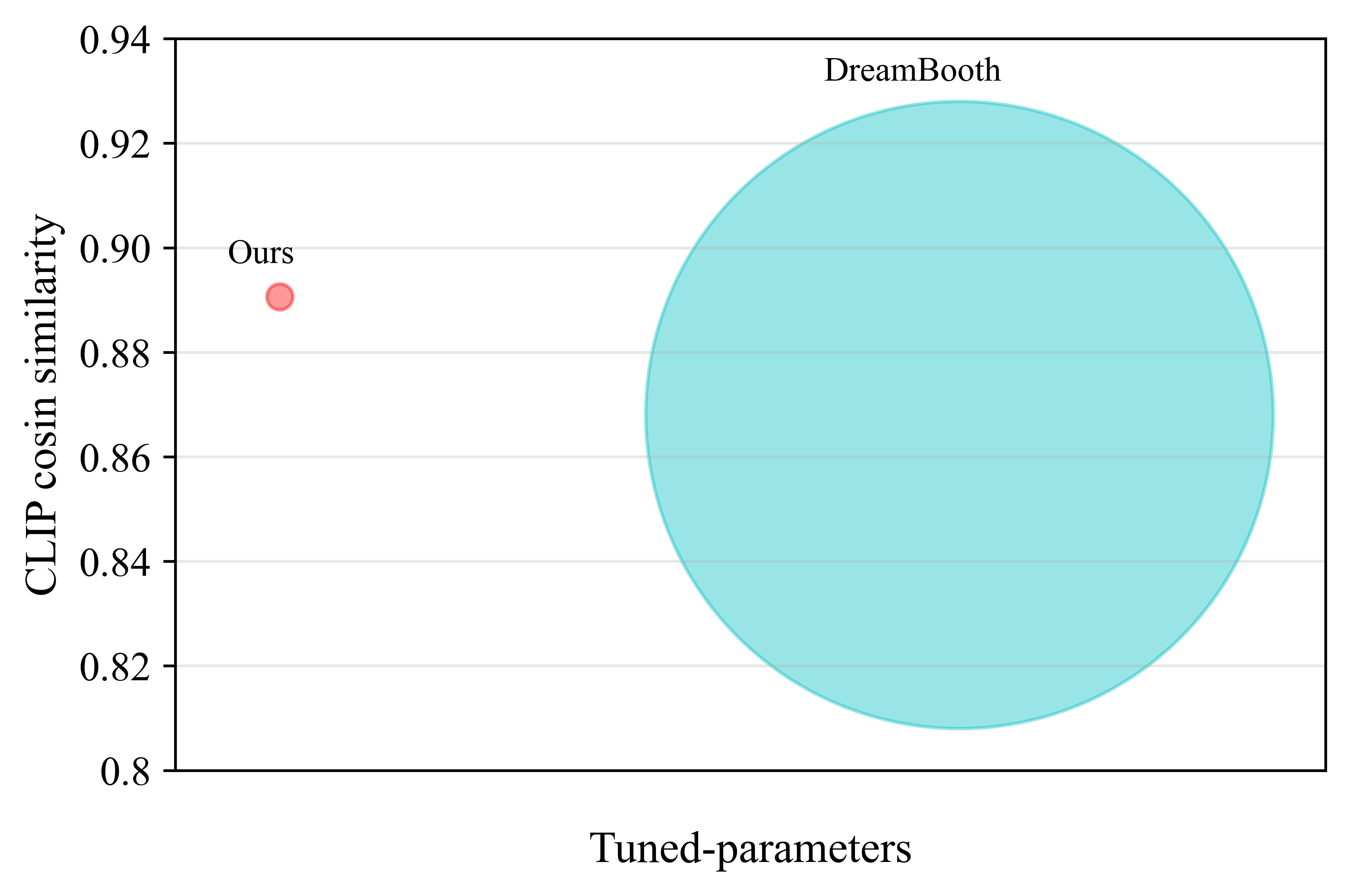
Built upon our study, our best setting could reach comparable if not better results with the fully fine-tuned method within 0.75% extra parameters on both the personalization task introduced in Dreambooth [32] and the task of fine-tuning on a small set of text-image pairs.
2 Background
2.1 Diffusion Models
Diffusion models learn the data distribution by reversing a noise-injection process
where corresponds to a step of noise injection. The transition of the reverse is approximated by a Gaussian model , where the optimal mean under the maximal likelihood estimation [2] is
Here and is the standard Gaussian noise injected to . To obtain the optimal mean, it is sufficient to estimate the conditional expectation via a noise prediction objective
where is the noise prediction network, and the optimal one satisfies according to the property of loss.
In practice, we often care conditional generation. To perform it with diffusion models, we only need to introduce the condition information to the noise prediction network during training
2.2 The Architecture in Stable Diffusion
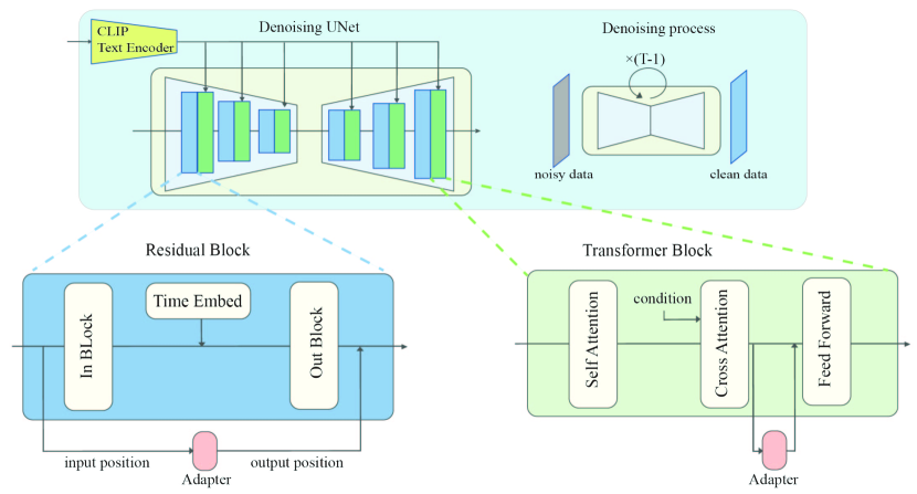
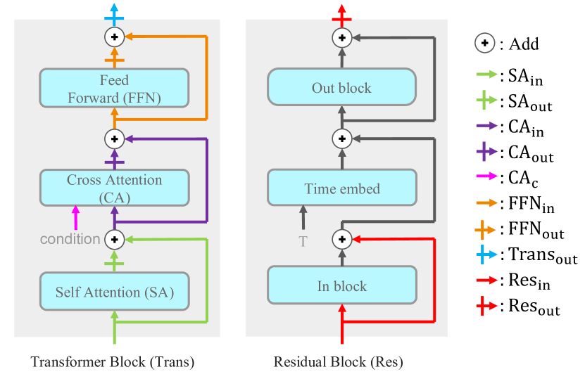
Currently, the most popular architecture for diffusion models is the U-Net-based architecture [14, 9, 30, 33, 31]. Specifically, the U-Net-based architecture in Stable Diffusion [31] is shown in Figure 3. The U-Net comprises stacked basic blocks, each containing a transformer block and a residual block.
In the transformer block, there are three types of sublayers: a self-attention layer, a cross attention layer, and a fully connected feed-forward network. The attention layer operates on queries , and key-value pairs :
| (1) |
where is the number of queries, is the number of key-value pairs is dimension of key, is the dimension of value. In the self-attention layer, is the only input. In the cross attention layer of conditioned diffusion model, there are two inputs and , where is the output from prior block and represents the condition information. The fully connected feed-forward network, which consists of two linear transformations with the ReLU activation function.:
| (2) |
where are the learnable weights, and , are the learnable biases.
The residual block consists of a sequence of convolutional layers and activations, where the time embedding is injected into the residual block by an addition operation.
2.3 Parameter-Efficient Transfer Learning
Transfer learning is a technique that leverages the knowledge learned from one task to improve the performance of a related task. The method of pre-training and then performing transfer learning on downstream tasks is widely used. However, traditional transfer learning approaches require large amounts of parameters, which is computationally expensive and memory-intensive.
Parameter-efficient transfer learning is first proposed in the area of natural language processing (NLP). The key idea of parameter-efficient transfer learning is to reduce the number of updated parameters. This could be done by updating a part of the model or adding extra small modules.
Some parameter-efficient transfer learning methods (such as adapter [16], LoRA [17]) choose to add extra small modules named adapters to the model. In contrast, other methods (prefix tuning [22], prompt-tuning [21]) prepend some learnable vectors to activations or inputs. Extensive study has validated that the efficient parameter fine-tuning method can achieve considerable results with a small number of parameters in the area of NLP.
3 Design Space of Parameter-Efficient Learning in Diffusion Models
Despite the success of parameter-efficient transfer learning in NLP, this technique is not fully understood in the area of diffusion models due to the existence of more components such as the residual block and cross-attention.
Before presenting our analysis on parameter-efficient tuning in diffusion models, we decompose the design space of adapters into three orthogonal factors – the input position, the output position, and the function form.
This work considers Stable Diffusion [31], since currently it is the only open-source large-scale diffusion model (see Figure 3 for its U-Net-based architecture). Below we elaborate the input position, the output position, and the function form based on the architecture of Stable Diffusion.
3.1 Input Position and Output Position
The input position is where the adapter’s input comes from, and the output position is where the adapter’s output goes. For a neat notation, as shown in Figure 4, the positions are named according to its neighboring layer. For example, represents that the position corresponds to the input of the self-attention layer, corresponds to the output of the transformer block, and corresponds to the condition input of the cross attention layer.
In our framework, the input position could be any one of the activation positions described in Figure 4. Thus, there are ten different options for the input position in total. As for output, some positions are equivalent since the addition is commutative. For example, putting output to is equivalent to putting output to . As a result, the options for the output position are reduced to seven in total. Another constraint is that the output position must be placed after the input position.
3.2 Function Form
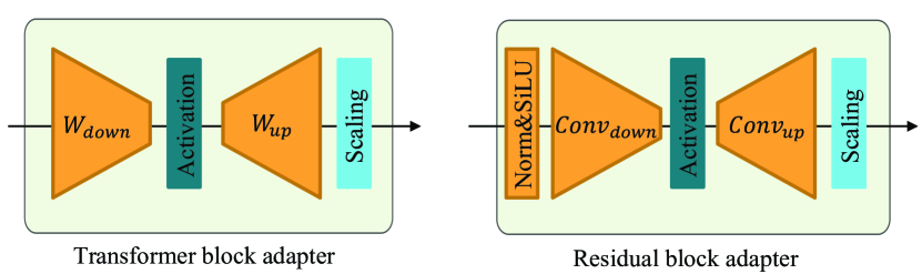
Function form describes how an adapter transfers the input into the output. We present the function form of adapters in the transformer block and residual block respectively (see Figure 5), where both consist of a down-sampling operator, an activation function, an up-sampling operator, and a scaling factor. The down-sampling operator reduces the dimension of the input and the up-sampling operator increases the dimension to ensure the output has the same dimension as the input. The output is further multiplied with a scaling factor to control its strength in influencing the original network.
Specifically, the transformer block adapter uses low-rank matrices and as the down-sampling and up-sampling operators respectively, and the residual block adapter employs 33 convolution layers and as the down-sampling and up-sampling operators respectively. Note that these convolution layers only change the number of channels without changing spatial size. Besides, the residual block adapter also processes its input with a group normalization [38] operator.
We include different activation functions and scaling factors in our design choice. The activation functions include , , , and identity operator as our design choices, and the scale factors include 0.5, 1.0, 2.0, 4.0.
4 Discover the Key Factor with Analysis of Variance
As mentioned earlier, finding the optimal solution in such a large discrete search space is a challenge. To discover which factor in the design space influences the performance the most, we quantify the correlation between model performance and factors by leveraging the one-way analysis of variance (ANOVA) method, which is widely used in many fields, including psychology, education, biology, and economics.
The main idea behind ANOVA is to partition the total variation in the data into two components: variation within groups (MSE) and variation between groups (MSB). MSB measures the difference between the group means, while the variation within groups measures the difference between individual observations and their respective group means. The statistical test used in ANOVA is based on the F-distribution, which compares the ratio of the variation between groups to the variation within groups (F-statistic). If the F-statistic is large enough, it suggests that there is a significant difference between the means of the groups, which indicates a strong correlation.
5 Experiments
We first present our experimental setup in Section 5.1. Then we analyze which factor in the design space is the most critical in Section 5.2. After discovering the importance of the input position, we present a detailed ablation study on it in Section 5.3. Finally, we present a comprehensive comparison between our best setting and DreamBooth (i.e., fine-tuning all parameters) in Section 5.4.
5.1 Setup
Tasks & datasets. We consider two transfer learning tasks in diffusion models characterized by different amount of data.
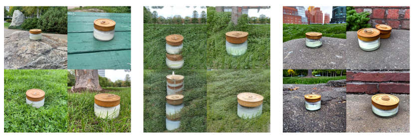
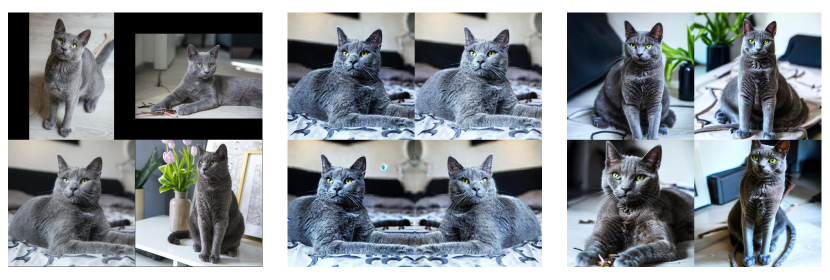
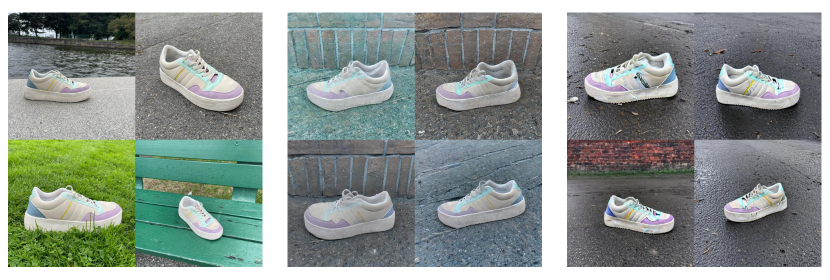
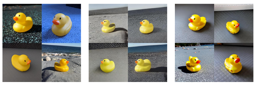
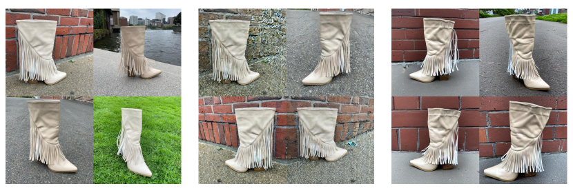
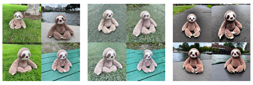
DreamBooth task. The first task is to personalize diffusion models with less than 10 input images, as proposed in DreamBooth [32]. We term it DreamBooth task for simplicity. The training dataset of DreamBooth consists of two sets of data: personalization data and regularization data. Personalization data is images of a specific object (e.g., a white dog) provided by the user. Regularization data is images of a general object similar to personalization data (e.g., dogs with different colors). Personalization data size is less than ten, and regularization data could be collected or generated by the model. DreamBooth uses rare token and class word to distinguish regularization data and personalization data. In particular, with regularization data, the prompt will be “a photo of ”; with personalization data, the prompt will be “a photo of ”. Where is a word to describe the general class of data (e.g., dog). We collect personalization data from both the Internet and live-action photography, and also with data from DreamBooth (33 in total). we use Stable Diffusion itself to generate corresponding regularization data conditioned on prompt “a photo of ”.
Fine-tuning task. The other task is to fine-tune on a small set of text-image pairs. We term it fine-tuning task for simplicity. Following [39], we consider fine-tuning on flower dataset [27] with 8189 images and use the same setting. We caption each image with the prompt “a photo of ”, where is the flower name of the image class.
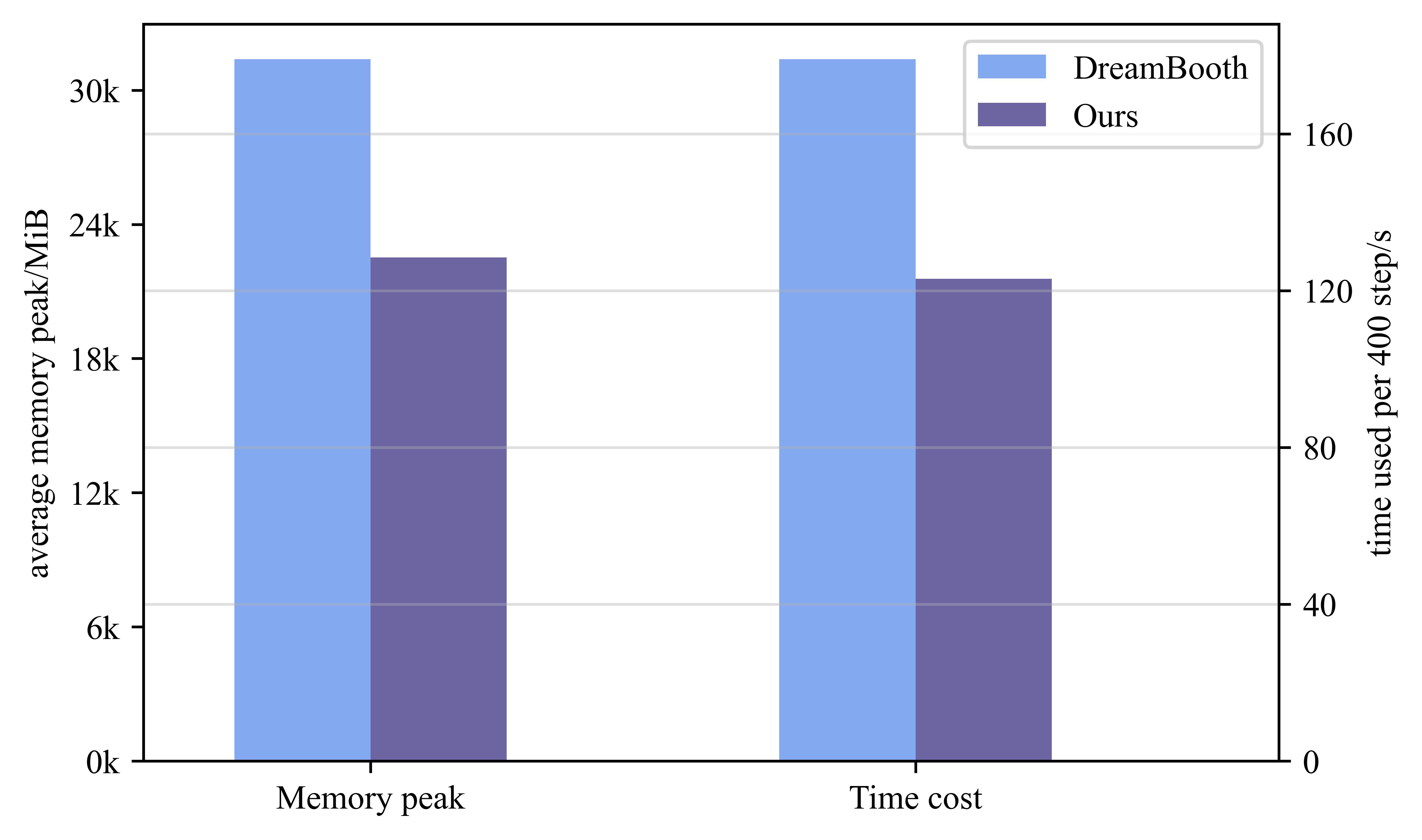
Tuning. We use AdamW [23] optimizer. For the DreamBooth task, we set the learning rate as 1e-4 which could let both DreamBooth and our method convergence around 1k step. fix the adapter size to 1.5M (0.17% of the UNet model), and train with 2.5k steps. For the task of fine-tuning on a small set of text-image pairs, we set the learning rate as 1e-5, fix the adapter size to 6.4M (0.72% of the UNet model), and train 60k steps.
Sampling. For a better sampling efficiency, we choose DPM-Solver [24] as the sampling algorithm with 25 sampling steps, and a classifier free guidance (cfg) [15] scale of . In some cases, we use cfg scale of for better image quality.
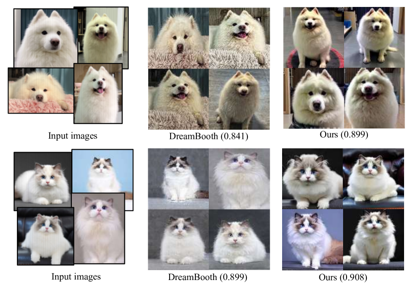
Evaluation. For the DreamBooth task, we evaluate faithfulness using the image distance in the CLIP space as proposed in [10]. Specifically, for each personalization target, we generate 32 images using the prompt: “A photo of ”. The metric is the mean pair-wise CLIP-space cosine-similarity (CLIP similarity) between the generated images and the images of the personalization training set.
For the task on fine-tuning on a small set of text-image pairs, we use the FID score [13] to evaluate the similarity between the training images and generated images. We randomly draw 5k prompts from the training set, use these prompts to generate images, and then compute FID by comparing generated images with training images.
5.2 Analysis of Variance (ANOVA) on the Design Space
Recall that we decompose the design space into factors of input position, output position, and function form. We perform ANOVA method (see Section 4 for details) on these design dimensions We consider the DreamBooth task for efficiency, since it requires fewer training steps.
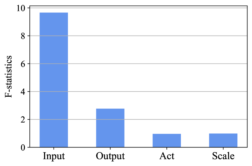
As shown in Figure 8, when grouped by input position, the F-statistic is large, which indicates that the input position is a critical factor to model’s performance. When grouped by output position, it shows a weak correlation. When grouped by function form (both activation function and scale factor), which have an F-statistic of around 1, indicating that the variability between groups is similar to the variability within groups, which suggests that there is no significant difference between the group means.
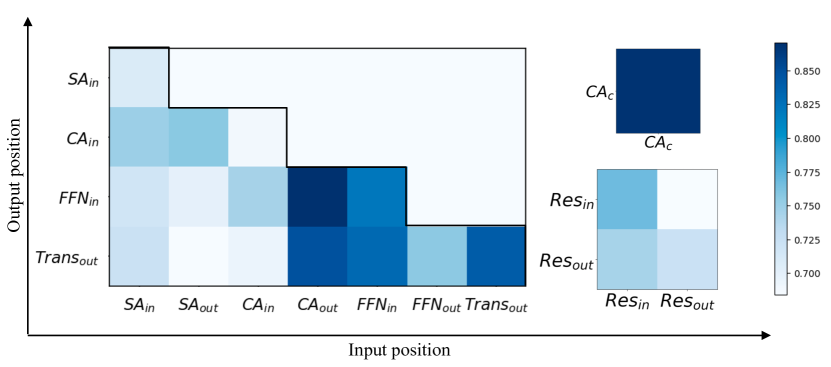
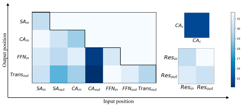
We further visualize the performance with different input positions and output positions. Figure 7 shows the results of the DreamBooth task. Figure 7 shows the FID results of the fine-tuning task.
As discussed above, we conclude that the input position of adapter is the key factor affecting the performance of parameter-efficient transfer learning.
5.3 Ablate the Input Position
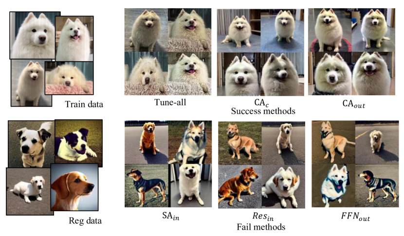
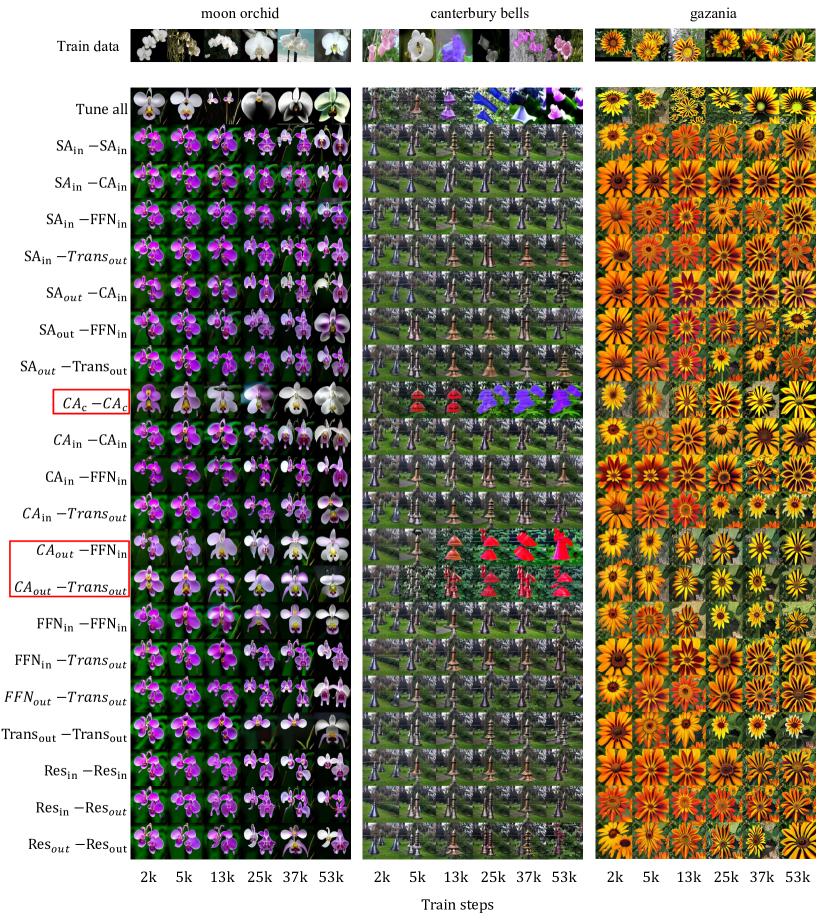
As shown in Figure 7 and Figure 7, we find that adapters with input position of or have a good performance on both tasks. In Figure 9, we present generated samples in the personalized diffusion models with different input positions of adapters. Adapters with input position at or are able to generate personalized images comparable to fine-tuning all parameters, while adapters with input position at other places do not.
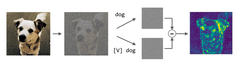
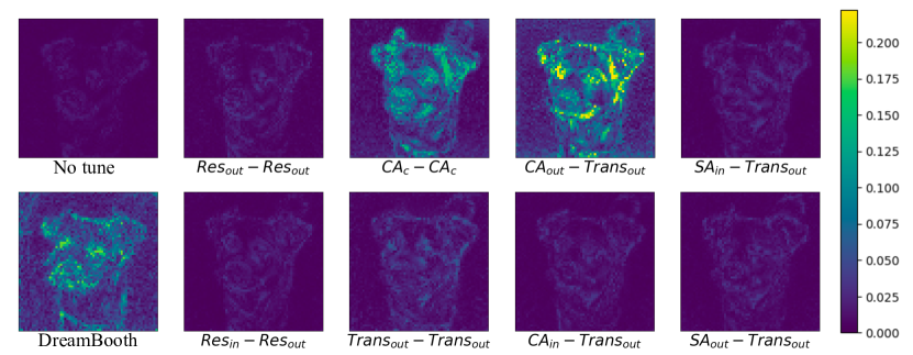
We further compute the difference between the noise prediction given prompt “a photo of ” and “a photo of ”. The pipeline is shown in Figure 10, where we firstly add noise to an image from the regularization data, use the U-Net to predict noise given the two prompts, and visualize the difference between the difference of two predicted noise. As shown in Figure 11, adapters with input position of or present a significant difference between the noise prediction.
5.4 Compare with DreamBooth
In this section, we compare our best setting (with input position at and output position as ) to DreamBooth, which fine-tunes all parameters in diffusion models.
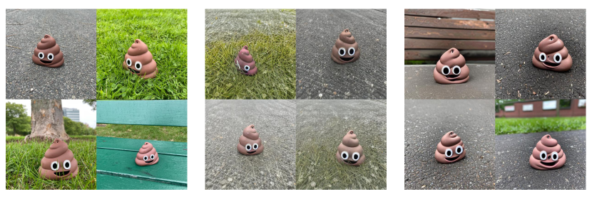
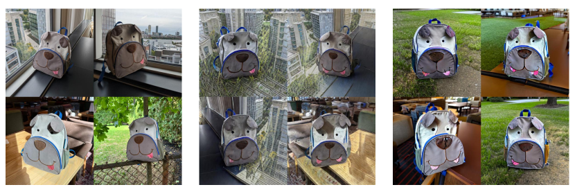
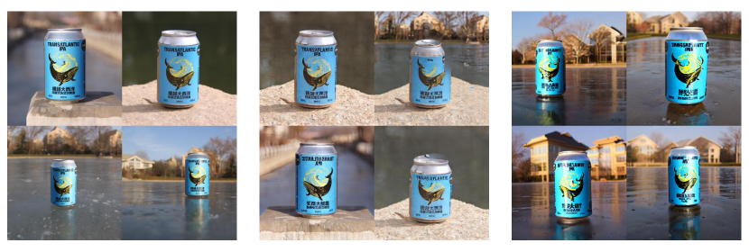
We show the results of each case on the DreamBooth task in Figure 12, which show that our method is better in most cases.
We also compare our best setting to the fully fine-tuned method in the fine-tuning task on the flower dataset. Our recipe reach FID of 24.49, which is better than 28.15 of the fully fine-tuned method.

6 Related Work
Personalization. Large-scale text-to-image diffusion models trained on web data can generate high-resolution and diverse images whose contents are controlled by the input text, but often lacks the ability for personalized generation on a certain object that the user desires. Recent work such as textual inversion [10] and DreamBooth [32] aims to address this by fine-tuning the diffusion model on a small set of images for the object. The textual inversion only tunes a word embedding. To obtain a stronger performance, DreamBooth tunes all parameters with a regularization loss to prevent overfitting.
Parameter-efficient transfer learning. Parameter-efficient transfer learning is originated from the area of NLP, such as adapter [16], prefix tuning [22], prompt tuning [21] and LoRA [17]. Specifically, adapter [16] inserts small low-rank multilayer perceptron (MLP) with nonlinear activation function between transformer block; prefix tuning [22] prepends tunable prefix vectors to the keys and values at each attention layer; prompt-tuning [21] simplifies prefix-tuning by adding tunable input word embeddings; LoRA [17] injects tunable low-rank matrices into the query and value projection matrices of the transformer block.
While these parameter-efficient transfer learning methods have different forms or motivations, recent work [12] proposes a unified view of these methods by designating a set of factors to describe the design space of parameter-efficient transfer learning in pure transformers [37]. These factors include modified representation, insertion form, functional form, and composition function. In contrast, our method focuses on U-Net with more components than pure transformers, leading to a larger design space. Besides, we use a simpler way to decompose the design space into orthogonal factors, i.e., the input position, the output position and the function form.
Transfer learning for diffusion models. There are methods that transfer the diffusion model to recognize a specific object or perform semantic editting [19, 32] by tuning the whole model. Previous work [39] tries to transfer a large diffusion model into an image-to-image model on small datasets, but the total number of parameters tuned is nearly half of the original model. [26, 40] transfers diffusion model to accept new conditions and introduces much more parameters than ours. Concurrent work [1] also performs parameter-efficient transfer learning on Stable Diffusion, their method could reach comparable results with fully fine-tuned method on DreamBooth [32] task, while their method is based on adding adapters on multiple positions at the same time, leading to a more complicated design space.
7 Conclusion
In this paper, we perform a systematical study on the design space of parameter-efficient transfer learning by inserting adapters in diffusion models. We decompose the design space of adapters into orthogonal factors – the input position, the output position and the function form. By performing Analysis of Variance (ANOVA), we discover the input position of adapters is the critical factor influencing the performance of downstream tasks. Then, we carefully study the choice of the input position, and we find that putting the input position after the cross-attention block can lead to the best performance, validated by additional visualization analyses. Finally, we provide a recipe for parameter-efficient tuning in diffusion models, which is comparable if not superior to the fully fine-tuned baseline (e.g., DreamBooth) with only 0.75 % extra parameters, across various customized tasks.
References
- [1] Low-rank adaptation for fast text-to-image diffusion fine-tuning. https://github.com/cloneofsimo/lora, 2022.
- [2] Fan Bao, Chongxuan Li, Jun Zhu, and Bo Zhang. Analytic-dpm: an analytic estimate of the optimal reverse variance in diffusion probabilistic models. In ICLR, 2022.
- [3] Fan Bao, Min Zhao, Zhongkai Hao, Peiyao Li, Chongxuan Li, and Jun Zhu. Equivariant energy-guided sde for inverse molecular design. ArXiv preprint, 2022.
- [4] Tom B. Brown, Benjamin Mann, Nick Ryder, Melanie Subbiah, Jared Kaplan, Prafulla Dhariwal, Arvind Neelakantan, Pranav Shyam, Girish Sastry, Amanda Askell, Sandhini Agarwal, Ariel Herbert-Voss, Gretchen Krueger, Tom Henighan, Rewon Child, Aditya Ramesh, Daniel M. Ziegler, Jeffrey Wu, Clemens Winter, Christopher Hesse, Mark Chen, Eric Sigler, Mateusz Litwin, Scott Gray, Benjamin Chess, Jack Clark, Christopher Berner, Sam McCandlish, Alec Radford, Ilya Sutskever, and Dario Amodei. Language models are few-shot learners, 2020.
- [5] Nanxin Chen, Yu Zhang, Heiga Zen, Ron J. Weiss, Mohammad Norouzi, and William Chan. Wavegrad: Estimating gradients for waveform generation. In ICLR, 2021.
- [6] Jooyoung Choi, Sungwon Kim, Yonghyun Jeong, Youngjune Gwon, and Sungroh Yoon. Ilvr: Conditioning method for denoising diffusion probabilistic models. In ICCV, 2021.
- [7] Aakanksha Chowdhery, Sharan Narang, Jacob Devlin, Maarten Bosma, Gaurav Mishra, Adam Roberts, Paul Barham, Hyung Won Chung, Charles Sutton, Sebastian Gehrmann, Parker Schuh, Kensen Shi, Sasha Tsvyashchenko, Joshua Maynez, Abhishek Rao, Parker Barnes, Yi Tay, Noam Shazeer, Vinodkumar Prabhakaran, Emily Reif, Nan Du, Ben Hutchinson, Reiner Pope, James Bradbury, Jacob Austin, Michael Isard, Guy Gur-Ari, Pengcheng Yin, Toju Duke, Anselm Levskaya, Sanjay Ghemawat, Sunipa Dev, Henryk Michalewski, Xavier Garcia, Vedant Misra, Kevin Robinson, Liam Fedus, Denny Zhou, Daphne Ippolito, David Luan, Hyeontaek Lim, Barret Zoph, Alexander Spiridonov, Ryan Sepassi, David Dohan, Shivani Agrawal, Mark Omernick, Andrew M. Dai, Thanumalayan Sankaranarayana Pillai, Marie Pellat, Aitor Lewkowycz, Erica Moreira, Rewon Child, Oleksandr Polozov, Katherine Lee, Zongwei Zhou, Xuezhi Wang, Brennan Saeta, Mark Diaz, Orhan Firat, Michele Catasta, Jason Wei, Kathy Meier-Hellstern, Douglas Eck, Jeff Dean, Slav Petrov, and Noah Fiedel. Palm: Scaling language modeling with pathways, 2022.
- [8] Jacob Devlin, Ming-Wei Chang, Kenton Lee, and Kristina Toutanova. Bert: Pre-training of deep bidirectional transformers for language understanding, 2018.
- [9] Prafulla Dhariwal and Alex Nichol. Diffusion models beat gans on image synthesis. ArXiv preprint, 2021.
- [10] Rinon Gal, Yuval Alaluf, Yuval Atzmon, Or Patashnik, Amit H. Bermano, Gal Chechik, and Daniel Cohen-Or. An image is worth one word: Personalizing text-to-image generation using textual inversion, 2022.
- [11] Ellen R Girden. ANOVA: Repeated measures. Number 84. Sage, 1992.
- [12] Junxian He, Chunting Zhou, Xuezhe Ma, Taylor Berg-Kirkpatrick, and Graham Neubig. Towards a unified view of parameter-efficient transfer learning. In International Conference on Learning Representations, 2022.
- [13] Martin Heusel, Hubert Ramsauer, Thomas Unterthiner, Bernhard Nessler, and Sepp Hochreiter. Gans trained by a two time-scale update rule converge to a local nash equilibrium. In I. Guyon, U. Von Luxburg, S. Bengio, H. Wallach, R. Fergus, S. Vishwanathan, and R. Garnett, editors, Advances in Neural Information Processing Systems, volume 30. Curran Associates, Inc., 2017.
- [14] Jonathan Ho, Ajay Jain, and Pieter Abbeel. Denoising diffusion probabilistic models. In NeurIPS, 2020.
- [15] Jonathan Ho and Tim Salimans. Classifier-free diffusion guidance. In NeurIPS, 2021.
- [16] Neil Houlsby, Andrei Giurgiu, Stanislaw Jastrzebski, Bruna Morrone, Quentin De Laroussilhe, Andrea Gesmundo, Mona Attariyan, and Sylvain Gelly. Parameter-efficient transfer learning for nlp. In International Conference on Machine Learning, pages 2790–2799. PMLR, 2019.
- [17] Edward J Hu, yelong shen, Phillip Wallis, Zeyuan Allen-Zhu, Yuanzhi Li, Shean Wang, Lu Wang, and Weizhu Chen. LoRA: Low-rank adaptation of large language models. In International Conference on Learning Representations, 2022.
- [18] Bahjat Kawar, Michael Elad, Stefano Ermon, and Jiaming Song. Denoising diffusion restoration models. arXiv preprint arXiv:2201.11793, 2022.
- [19] Bahjat Kawar, Shiran Zada, Oran Lang, Omer Tov, Huiwen Chang, Tali Dekel, Inbar Mosseri, and Michal Irani. Imagic: Text-based real image editing with diffusion models, 2022.
- [20] Zhifeng Kong, Wei Ping, Jiaji Huang, Kexin Zhao, and Bryan Catanzaro. Diffwave: A versatile diffusion model for audio synthesis. In ICLR, 2021.
- [21] Brian Lester, Rami Al-Rfou, and Noah Constant. The power of scale for parameter-efficient prompt tuning. In Proceedings of the 2021 Conference on Empirical Methods in Natural Language Processing, pages 3045–3059, Online and Punta Cana, Dominican Republic, Nov. 2021. Association for Computational Linguistics.
- [22] Xiang Lisa Li and Percy Liang. Prefix-tuning: Optimizing continuous prompts for generation. In Proceedings of the 59th Annual Meeting of the Association for Computational Linguistics and the 11th International Joint Conference on Natural Language Processing (Volume 1: Long Papers), pages 4582–4597, Online, Aug. 2021. Association for Computational Linguistics.
- [23] Ilya Loshchilov and Frank Hutter. Decoupled weight decay regularization. In International Conference on Learning Representations, 2019.
- [24] Cheng Lu, Yuhao Zhou, Fan Bao, Jianfei Chen, Chongxuan Li, and Jun Zhu. DPM-solver: A fast ODE solver for diffusion probabilistic model sampling in around 10 steps. In Alice H. Oh, Alekh Agarwal, Danielle Belgrave, and Kyunghyun Cho, editors, Advances in Neural Information Processing Systems, 2022.
- [25] Chenlin Meng, Yang Song, Jiaming Song, Jiajun Wu, Jun-Yan Zhu, and Stefano Ermon. Sdedit: Image synthesis and editing with stochastic differential equations. In ICLR, 2022.
- [26] Chong Mou, Xintao Wang, Liangbin Xie, Jian Zhang, Zhongang Qi, Ying Shan, and Xiaohu Qie. T2i-adapter: Learning adapters to dig out more controllable ability for text-to-image diffusion models, 2023.
- [27] M-E. Nilsback and A. Zisserman. Automated flower classification over a large number of classes. In Proceedings of the Indian Conference on Computer Vision, Graphics and Image Processing, Dec 2008.
- [28] Ben Poole, Ajay Jain, Jonathan T. Barron, and Ben Mildenhall. Dreamfusion: Text-to-3d using 2d diffusion, 2022.
- [29] Colin Raffel, Noam Shazeer, Adam Roberts, Katherine Lee, Sharan Narang, Michael Matena, Yanqi Zhou, Wei Li, and Peter J. Liu. Exploring the limits of transfer learning with a unified text-to-text transformer. Journal of Machine Learning Research, 21(140):1–67, 2020.
- [30] Aditya Ramesh, Prafulla Dhariwal, Alex Nichol, Casey Chu, and Mark Chen. Hierarchical text-conditional image generation with clip latents, 2022.
- [31] Robin Rombach, Andreas Blattmann, Dominik Lorenz, Patrick Esser, and Björn Ommer. High-resolution image synthesis with latent diffusion models, 2021.
- [32] Nataniel Ruiz, Yuanzhen Li, Varun Jampani, Yael Pritch, Michael Rubinstein, and Kfir Aberman. Dreambooth: Fine tuning text-to-image diffusion models for subject-driven generation. 2022.
- [33] Chitwan Saharia, William Chan, Saurabh Saxena, Lala Li, Jay Whang, Emily Denton, Seyed Kamyar Seyed Ghasemipour, Burcu Karagol Ayan, S. Sara Mahdavi, Rapha Gontijo Lopes, Tim Salimans, Jonathan Ho, David J Fleet, and Mohammad Norouzi. Photorealistic text-to-image diffusion models with deep language understanding, 2022.
- [34] Chitwan Saharia, Jonathan Ho, William Chan, Tim Salimans, David J Fleet, and Mohammad Norouzi. Image super-resolution via iterative refinement. IEEE Transactions on Pattern Analysis and Machine Intelligence, 2022.
- [35] Jascha Sohl-Dickstein, Eric A. Weiss, Niru Maheswaranathan, and Surya Ganguli. Deep unsupervised learning using nonequilibrium thermodynamics. In ICLR, 2015.
- [36] Yang Song, Jascha Sohl-Dickstein, Diederik P. Kingma, Abhishek Kumar, Stefano Ermon, and Ben Poole. Score-based generative modeling through stochastic differential equations. In ICLR, 2021.
- [37] Ashish Vaswani, Noam Shazeer, Niki Parmar, Jakob Uszkoreit, Llion Jones, Aidan N. Gomez, Lukasz Kaiser, and Illia Polosukhin. Attention is all you need. In NeurIPS, 2017.
- [38] Yuxin Wu and Kaiming He. Group normalization. CoRR, abs/1803.08494, 2018.
- [39] Fuming You and Zhou Zhao. Transferring pretrained diffusion probabilistic models, 2023.
- [40] Lvmin Zhang and Maneesh Agrawala. Adding conditional control to text-to-image diffusion models, 2023.
- [41] Min Zhao, Fan Bao, Chongxuan Li, and Jun Zhu. Egsde: Unpaired image-to-image translation via energy-guided stochastic differential equations. In NeurIPS, 2022.
Experiment detail. In the Figure-6 of the main paper, we find no significant performance changes after 1k steps of tuning in our main, so we use an averaged CLIP similarity between 1k and 2.5k training steps at an interval of 500 steps as the final metric.
In the Figure-7 of the main paper, due to methods convergence on different training steps, we use minimum FID in the training process as the final metric.