Implicit Peer Triplets in Gradient-Based Solution Algorithms for ODE Constrained Optimal Control

Abstract

It is common practice to apply gradient-based optimization algorithms to numerically solve large-scale ODE constrained optimal control problems. Gradients of the objective function are most efficiently computed by approximate adjoint variables. High accuracy with moderate computing time can be achieved by such time integration methods that satisfy a sufficiently large number of adjoint order conditions and supply gradients with higher orders of consistency. In this paper, we upgrade our former implicit two-step Peer triplets constructed in [Algorithms, 15:310, 2022] to meet those new requirements. Since Peer methods use several stages of the same high stage order, a decisive advantage is their lack of order reduction as for semi-discretized PDE problems with boundary control. Additional order conditions for the control and certain positivity requirements now intensify the demands on the Peer triplet. We discuss the construction of $4$-stage methods with order pairs $(4,3)$ and $(3,3)$ in detail and provide three Peer triplets of practical interest. We prove convergence for $s$-stage methods, for instance, order $s$ for the state variables even if the adjoint method and the control satisfy the conditions for order $s-1$, only. Numerical tests show the expected order of convergence for the new Peer triplets.

Key words. Implicit Peer two-step methods, nonlinear optimal control, gradient-based optimization, first-discretize-then-optimize, discrete adjoints

1 Introduction

The numerical solution of optimal control problems governed by time-dependent differential equations is still a challenging task in designing and analyzing higher-order time integrators. An essential solution strategy is the so called first-discretize-then-optimize approach, where the continuous control problem is first discretized into a nonlinear programming problem which is then solved by state-of-the-art gradient-based optimization algorithm. Nowadays this direct approach is the most commonly used method due to its easy applicability and robustness. Consistent gradients of the objective function are derived from control, state and adjoint variables given by first-order necessary conditions of Karush-Kuhn-Tucker type, and are used in an iterative minimization algorithm to calculate the wanted optimal control. In this solution strategy, the unique gain of higher-order time integrators is twofold: increasing the efficiency in computing time by the use of larger and fewer time steps and, even more important for large-scale problems, thus reducing at the same time the memory requirement caused by the necessity to store all variables for the computation of gradients.

There are one-step as well as multistep time integrators in common use to solve ODE constrained optimal control problems. Symplectic Runge-Kutta methods [5, 20, 25] and backward differentiation formulas [1, 4] are prominent classes, but also partitioned and implicit-explicit Runge–Kutta methods [14, 22] and explicit stabilized Runge-Kutta-Chebyshev methods [2] have been proposed. However, fully implicit one-step methods often request the solution of large systems of coupled stages and might suffer from serious order reduction due to their lower stage order. This is especially the case when they are applied to semi-discretized PDEs with general time-dependent boundary conditions arising from boundary control problems [18, 23]. In general, further consistency conditions have to be satisfied [11, 19] in order the achieve a higher classical order for the discrete adjoint variables. Multistep methods avoid order reduction and have a simple structure, but higher order comes with restricted stability properties and adjoint initialization steps are usually inconsistent approximations. Moreover, the appropriate approximation of initial values and its structural consequences for the adjoint variables are further unsolved inherent difficulties that have limited the application of higher-order multistep methods for optimal control problems in a first-discretize-then-optimize solution strategy.

Recently, we have proposed a new class of implicit two-step Peer triplets that aggregate the attractive properties of one- and multistep methods through the use of several stages of one and the same high order and at the same time avoid their deficiencies by their two-step form [16, 17, 18]. The incorporation of different but matching start and end steps increases the flexibility of Peer methods for the solution of optimal control problems, especially also allowing higher-order approximations of the control, adjoint variables and the gradient of the objective function.

The class of $s$-stage implicit two-step Peer methods was introduced in [26] in linearly implicit form to solve stiff ODEs of the form $y^{\prime}(t)=f(y(t))$, $y_{0}=y(0)$, $y\in{\mathbb{R}}^{m}$. Later, the methods were simplified as implicit two-step schemes

$$Y_{n}= \;(Q\otimes I_{m})Y_{n-1}+h(R\otimes I_{m})F(Y_{n}),\;n=0,1,\ldots,$$ (1)

where the constant time step $h>0$ will be considered here. An application of (1) to large scale problems with Krylov solvers was discussed in [3]. The stage solutions $Y_{n}=(Y_{ni})_{i=1}^{s}$ are approximations of $(y(t_{n}+c_{i}h))_{i=0}^{s}$ with equal accuracy and stability properties, which motivates the attribute peer and is the key for avoiding order reduction. The off-step nodes $c_{1},\ldots,c_{s}$ are associated with the interval $[0,1]$ but some may lie outside. In (1), $R\in{\mathbb{R}}^{s\times s}$ is lower triangular and invertible, $Q\in{\mathbb{R}}^{s\times s}$, $I_{m}\in{\mathbb{R}}^{m\times m}$ is the identity matrix, and $F(Y_{n})=(f(Y_{ni}))_{i=1}^{s}$. Note that the stages $Y_{ni}$ can be successively computed for $i=1,\ldots,s$ due to the triangular structure of $R$. Several variants of Peer methods have been developed and successfully applied to a broad class of differential equations, e.g. [9, 15, 21, 24, 27, 28].

The application of Peer methods to optimal control problems requires a couple of modifications. A first direct attempt in [29] was unsatisfactory, mainly due to the restricted, first-order approximation of the adjoint variables. In [16], we found that the general redundant formulation of the above standard Peer method,

$$(A\otimes I_{m})Y_{n}= \;(B\otimes I_{m})Y_{n-1}+h(K\otimes I_{m})F(Y_{n}),\;n=0,1,\ldots,$$ (2)

with invertible lower triangular matrix $A\in{\mathbb{R}}^{s\times s}$ and diagonal matrix $K\in{\mathbb{R}}^{s\times s}$ is admittedly equivalent in terms of the state variables to (1), but surprisingly not for the adjoint variables with the same coefficients $Q,R$. The additional degrees of freedom given by $K$ together with a careful design of a start and end method with different coefficient matrices laid the foundation for improved Peer triplets with higher-order convergence. Triplets with good stability properties could be found [17]. Formulation (2) will also be the starting point in this paper. In contrast to our former approach in [16, 17], where the control has been eliminated and a boundary value problem has been solved, we now compute the optimal control in an iterative procedure, making use of gradients of the objective function.

An important advantage of the state and adjoint approximations $Y_{ni}\approx y(t_{n}+c_{i}h)$ and $P_{ni}\approx p(t_{n}+c_{i}h)$ in the discrete time points $t_{n}+c_{i}h$ (see the next Chapter for the details of the notation) with equal high accuracy is the opportunity to simply use the discrete control variables

$$U_{ni}=\Phi(Y_{ni},P_{ni})\approx u(t_{n}+c_{i}h),\;i=1,\ldots,s,\,n=0,1,\ldots,$$ (3)

in a gradient-based optimization algorithm. Although, the function $\Phi$ is only implicitly given, the higher order of $Y_{ni}$ and $P_{ni}$ is directly transferable to the control vector $U_{ni}$. Interpolation in time is easily realizable, the data structure keeps simple. However, additional order conditions for the control derived from (3) and positivity requirements for column sums in the matrix triplet $(K_{0},K,K_{N})$, where $K_{0}$ and $K_{N}$ are the matrices for the start and end method, intensify the demands on the Peer methods in the triplet. The arising bottlenecks in the design caused by stronger entanglement of all matrices must be resolved by a more sophisticated analysis.

The paper is organized as follows. In Chapter 2, we formulate the optimal control problem and define its discretization. The gradient of the cost function is derived in Chapter 3. Order conditions and their algebraic consequences are discussed in Chapter 4. Two classes of four-stage Peer triplets are studied in Chapter 5 and Chapter 6 and three triplets of practical interest are constructed. In Chapter 7, we give a detailed convergence proof for unconstrained controls. Numerical examples collected in Chapter 8 illustrate the theoretical findings. The paper concludes with a summary in Chapter 9.

2 The optimal control problem and its discretization

We are interested in the numerical solution of the following ODE-constrained nonlinear optimal control problem:

$$\mbox{minimize }{\cal C}\big{(}y(T)\big{)}$$ (4)

$$\mbox{subject to }y^{\prime}(t)= \,f\big{(}y(t),u(t)\big{)},\quad u(t)\in U_{ad},\;t\in(0,T],$$ (5)

$$y(0)= \,y_{0},$$ (6)

where the state $y(t)\in{\mathbb{R}}^{m}$, the control $u(t)\in{\mathbb{R}}^{d}$, $f:{\mathbb{R}}^{m}\times{\mathbb{R}}^{d}\mapsto{\mathbb{R}}^{m}$, the objective function ${\cal C}:{\mathbb{R}}^{m}\mapsto{\mathbb{R}}$, and the set of admissible controls $U_{ad}\subset{\mathbb{R}}^{d}$ is closed and convex. Introducing for any $u\in U_{ad}$ the normal cone mapping

$$N_{U}(u)= \,\{w\in{\mathbb{R}}^{d}:w^{T}(v-u)\leq 0\mbox{ for all }v\in U_{ad}\},$$ (7)

the first-order optimality conditions read [11, 30]

$$y^{\prime}(t)= \,f\big{(}y(t),u(t)\big{)},\quad t\in(0,T],\quad y(0)=y_{0},$$ (8)

$$p^{\prime}(t)= \,-\nabla_{y}f\big{(}y(t),u(t)\big{)}^{\sf T}p(t),\quad t\in[0,T),\quad p(T)=\nabla_{y}{{\cal C}}\big{(}y(T)\big{)}^{\sf T},$$ (9)

$$\,-\nabla_{u}f\big{(}y(t),u(t)\big{)}^{\sf T}p(t)\in N_{U}\big{(}u(t)\big{)},\quad t\in[0,T].$$ (10)

Under appropriate regularity conditions, there exists a local solution $(y,u)$ of the optimal control problem (4)-(6) and a Lagrange multiplier $p$ such that the first-order optimality conditions (8)-(10) are necessarily satisfied at $(y,u,p)$. If, in addition, the Hamiltonian $H(y,u,p):=p^{\sf T}f(y,u)$ satisfies a coercivity assumption, then these conditions are also sufficient [11]. The control uniqueness property introduced in [11] yields the existence of a locally unique minimizer $u=u(y,p)$ of the Hamiltonian over all $u\in U_{ad}$, if $(\hat{y},\hat{p})$ is sufficiently close to $(y,p)$.

Many other optimal control problems can be transformed to the Mayer form ${\cal C}(y(T))$ which only uses terminal solutions. For example, terms given in the Lagrange form

$${\cal C}_{L}(y,u):= \;\int_{0}^{T}l(y(t),u(t))\,dt$$ (11)

can be equivalently reduced to the Mayer form by adding a new differential equation $y_{m+1}^{\prime}(t)=l(y(t),u(t))$ and initial values $y_{m+1}(0)=0$ to the constraints. Then (11) simply reduces to $y_{m+1}(T)$.

On a time grid $\{t_{0},\ldots,t_{N}\}\subset[0,T]$ with fixed step size length $h=t_{n+1}-t_{n}$ Peer methods use $s$ stage-approximations $Y_{ni}\approx y(t_{ni})$ and $U_{ni}\approx u(t_{ni})$ per time step at points $t_{ni}=t_{n}+c_{i}h$, $i=1,\ldots,s,$ associated with fixed nodes $c_{1},\ldots,c_{s}$. All $s$ stages share the same properties like a common high stage order equal to the global order preventing order reduction. Applying the two-step Peer method for $n\geq 1$ and an exceptional starting step for $n=0$ to the problem (5)–(6) we get the discrete constraint nonlinear optimal control problem

$$\mbox{minimize }{\cal C}\big{(}y_{h}(T)\big{)}$$ (12)

$$\mbox{subject to }A_{0}Y_{0}= \,a\otimes y_{0}+hK_{0}F(Y_{0},U_{0}),$$ (13)

$$A_{n}Y_{n}= \,B_{n}Y_{n-1}+hK_{n}F(Y_{n},U_{n}),\ n=1,\ldots,N,$$ (14)

with long vectors $Y_{n}=(Y_{ni})_{i=1}^{s}\in{\mathbb{R}}^{sm}$, $U_{n}=(U_{ni})_{i=1}^{s}\in{\mathbb{R}}^{sd}$, and $F(Y_{n},U_{n})=\big{(}f(Y_{ni},U_{ni})\big{)}_{i=1}^{s}$. Further, $y_{h}(T)=(w^{T}\otimes I)Y_{N}\approx y(T)$, $a,w\in{\mathbb{R}}^{s}$, $A_{n},B_{n},K_{n}\in{\mathbb{R}}^{s\times s}$, and $I\in{\mathbb{R}}^{m\times m}$ being the identity matrix. As a change to the introduction, we will use the same symbol for a coefficient matrix like $A$ and its Kronecker product $A\otimes I$ as a mapping from the space ${\mathbb{R}}^{sm}$ to itself. Throughout the paper, $e_{i}$ denotes the $i$-th cardinal basis vector and $\mbox{1\hskip-2.40005ptl}:=(1,\ldots,1)^{\sf T}\in{\mathbb{R}}^{s}$, sometimes with an additional index indicating the space dimension.

On each subinterval $[t_{n},t_{n+1}]$, Peer methods may be defined by three coefficient matrices $A_{n},B_{n},K_{n}$, where $A_{n}$ is assumed to be nonsingular. For practical reasons, this general version will not be used. We choose a fixed Peer method $(A_{n},B_{n},K_{n})\equiv(A,B,K)$, $n\!=\!1,\ldots,N-1$, in the inner grid points with lower triangular $A$, which allows a consecutive computation of the solution vectors $Y_{ni}$, $i\!=\!1,\ldots,s$, in (13), (14). Exceptional coefficients $(A_{0},K_{0})$ and $(A_{N},B_{N},K_{N})$ in the first and last forward steps are taken to allow for a better approximation in the initial step and of the end conditions.

The first order optimality conditions now read

$$A_{0}Y_{0}= \,a\otimes y_{0}+hK_{0}F(Y_{0},U_{0}),$$ (15)

$$A_{n}Y_{n}= \,B_{n}Y_{n-1}+hK_{n}F(Y_{n},U_{n}),\ n=1,\ldots,N,$$ (16)

$$A_{N}^{\sf T}P_{N}= \,w\otimes p_{h}(T)+h\nabla_{Y}F(Y_{N},U_{N})^{\sf T}K_{N}^{\sf T}P_{N},$$ (17)

$$A_{n}^{\sf T}P_{n}= \,B_{n+1}^{\sf T}P_{n+1}+h\nabla_{Y}F(Y_{n},U_{n})^{\sf T}K_{n}^{\sf T}P_{n},\ 0\leq n\leq N-1,$$ (18)

$$\,-h\nabla_{U}F(Y_{n},U_{n})^{\sf T}K_{n}^{\sf T}P_{n}\in N_{U^{s}}\big{(}U_{n}\big{)},\ 0\leq n\leq N.$$ (19)

Here, $p_{h}(T)=\nabla_{y}{\cal C}\big{(}y_{h}(T)\big{)}^{\sf T}$ and the Jacobians of $F$ are block diagonal matrices $\nabla_{Y}F(Y_{n},U_{n})=\,\mbox{diag}_{i}\big{(}\nabla_{Y_{ni}}f(Y_{ni},U_{ni})\big{)}$ and $\nabla_{U}F(Y_{n},U_{n})=\,\mbox{diag}_{i}\big{(}\nabla_{U_{ni}}f(Y_{ni},U_{ni})\big{)}$. The generalized normal cone mapping $N_{U^{s}}\big{(}U_{n}\big{)}$ is defined by

$$N_{U^{s}}(u)= \,\left\{w\in{\mathbb{R}}^{sd}:w^{T}(v-u)\leq 0\mbox{ for all }v\in U_{ad}^{s}\subset{\mathbb{R}}^{sd}\right\}.$$ (20)

If $K_{n}:=(\kappa_{ij}^{[n]})$ is diagonal and $\kappa_{ii}^{[n]}=0$, then (19) is satisfies automatically for stage $i\in\{1,\ldots,s\}$. Assuming otherwise $k_{ni}:=e_{i}^{T}K_{n}^{T}\mbox{{1\hskip-2.40005ptl}}\not=0$, and defining

$$Q_{ni}:=\frac{1}{k_{ni}}\,\sum_{j}\kappa_{ji}^{[n]}P_{nj},\ 0\leq n\leq N,\ i=1,\ldots,s,$$ (21)

(19) can be equivalently reformulated as

$$-k_{ni}\,\nabla_{U_{ni}}f(Y_{ni},U_{ni})^{\sf T}Q_{ni}\in N_{U}\big{(}U_{ni}\big{)},\ 0\leq n\leq N,\ i=1,\ldots,s.$$ (22)

Note that $Q_{ni}=P_{ni}$, if the matrix $K_{n}$ is diagonal. A severe new restriction on the Peer triplet comes from the need to preserve the correct sign in (22) requiring that $k_{ni}>0$. Then, we can divide by it and the control uniqueness property guarantees the existence of a local minimizer $U_{ni}$ of the Hamiltonian $H(Y_{ni},U,Q_{ni})$ over all $U\in U_{ad}$ since $Q_{ni}$ can be seen as an approximation to the multiplier $P_{ni}\approx p(t_{n}+c_{i}h)$. Such positivity conditions also arise in the context of classical Runge-Kutta methods or W-methods, see e.g. [11, Theorem 2.1] and [19, Chapter 5.2].

The need to sacrifice the triangular resp. diagonal form of the matrix coefficients $A_{n},K_{n}$ in the boundary steps comes from the fact that the starting steps (15), and backwards (17) are single-step methods with $s$ outputs. With a triangular form of $A_{0},A_{N}$ and $K_{0},K_{N}$ their first stages (backward for $n=N$) would represent simple implicit Euler steps with a local order limited to 2, see Section 5 in [16] for a discussion.

3 The gradient of the cost function

We first introduce the vector of control values for the entire interval $[0,T]$

$$U= \,(U_{01}^{\sf T},\ldots,U_{0s}^{\sf T},U_{11}^{\sf T},\ldots,U_{Ns}^{\sf T})^{\sf T}\in{\mathbb{R}}^{sd(N+1)}$$ (23)

and let ${\cal C}(U):={\cal C}(y_{h}(U))$ be the cost function associated with these controls. The first order system (15)–(19) provides a convenient way to compute the gradient of ${\cal C}(U)$ with respect to $U$. Following the approach in [12], we find

$$\nabla_{U_{ni}}{\cal C}(U)= \,h\nabla_{U_{ni}}f(Y_{ni},U_{ni})^{\sf T}(e_{i}^{\sf T}K_{n}^{\sf T}\otimes I)P_{n},\ 0\leq n\leq N,\ i=1,\ldots,s,$$ (24)

where all approximations $(Y_{n},P_{n})$ are computable by a forward-backward marching scheme. The state variables $Y_{n}$ are obtained from the discrete state equations (15)–(16) for $n=0,\ldots,N$, using the given values of the control vector $U$. Then, using the updated values $Y_{n}$ one computes $p_{h}(T)=\nabla_{y}{\cal C}\big{(}y_{h}(T)\big{)}^{\sf T}$ with $y_{h}(T)=(w^{\sf T}\otimes I)Y_{N}$ before marching the steps (17)–(18) backwards for $n=N,\ldots,0$, solving the discrete costate equations for all $P_{n}$.

The gradients from (24) can now be employed in gradient-based optimization algorithms which have been developed extensively since the 1950s. Many good algorithms are now available to solve nonlinear optimization problems in an iterative procedure

$$U^{(k+1)}:= \,U^{(k)}+\triangle U^{(k)},\quad k=0,1,\ldots$$ (25)

starting from an initial estimate $U^{(0)}$ for the control vector. Evaluating the objective function, its gradient and, in some cases, its Hessian, an efficient update $\triangle U^{(k)}$ of the control can be computed. Based on the principle (25), several good algorithms have been implemented in commercial software packages like Matlab, Mathematica, and others. We will use the Matlab routine fmincon in our numerical experiments. It offers several optimization algorithms including interior-point [7] and trust-region-reflective [8] for large-scale sparse problems with continuous objective function and first derivatives.

Since the optimal control $u(t)$ minimizes the Hamiltonian $H(y,u,p)=p^{\sf T}f(y,u)$, we may compute an improved approximation of the control by the following minimum principle

$$U^{\star}_{ni}=\operatorname*{arg\,min}_{u\in U_{ad}}H(Y_{ni},u,P_{ni}),\quad 0\leq n\leq N,\ i=1,\ldots,s,$$ (26)

if $Y_{ni}$ or $P_{ni}$ are approximations of higher-order. We note that the function $\Phi$ in (3) provides the solution in (26), when $H$ is replaced by its discrete approximation defined by the Peer triplet.

4 Order conditions for the Peer triplet in the unconstrained case

We recall the conditions for local order $r\leq s$ for the forward schemes and order $q\leq s$ for the adjoint schemes, see [16, 17]. These conditions use the Vandermonde matrices $V_{q}:=(\mbox{1\hskip-2.40005ptl},{\bf c},{\bf c}^{2},\ldots,{\bf c}^{q-1})\in{\mathbb{R}}^{s\times q}$ with the column vector of nodes ${\bf c}=(c_{i})_{i=1}^{s}\in{\mathbb{R}}^{s}$, and the nonsingular Pascal matrix ${\cal P}_{q}=\big{(}{j-1\choose i-1}\big{)}=\exp(\tilde{E}_{q})\in{\mathbb{R}}^{q\times q}$ where $\tilde{E}=\big{(}i\delta_{i+1,j}\big{)}\in{\mathbb{R}}^{q\times q}$ is nilpotent. There are 5 conditions for the forward scheme and its adjoint method:

$$A_{0}V_{r}= \,ae_{1}^{\sf T}+K_{0}V_{r}\tilde{E}_{r},\ n=0,$$ (27)

$$A_{n}V_{r}= \,B_{n}V_{r}{\cal P}_{r}^{-1}+K_{n}V_{r}\tilde{E}_{r},\ 1\leq n\leq N,$$ (28)

$$w^{\sf T}V_{r}= \,\mbox{1\hskip-2.40005ptl}^{\sf T},$$ (29)

$$A_{n}^{\sf T}V_{q}= B_{n+1}^{\sf T}V_{q}{\cal P}_{q}-K_{n}^{\sf T}V_{q}\tilde{E}_{q},\ 0\leq n\leq N-1,$$ (30)

$$A_{N}^{\sf T}V_{q}= w\mbox{1\hskip-2.40005ptl}^{\sf T}-K_{N}^{\sf T}V_{q}\tilde{E}_{q},\ n=N.$$ (31)

We remind that the coefficient matrices from interior grid intervals belong to a standard scheme $(A_{n},B_{n},K_{n})\equiv(A,B,K),\,1\leq n\leq N-1$. The whole triplet consists of 8 coefficient matrices $(A_{0},K_{0}),\,(A,B,K),\,(A_{N},B_{N},K_{N})$.

Next, we focus on the new optimality condition (19) in the unconstrained case with $N_{U}=\{0\}$. It reads stage-wise

$$\nabla_{u}f(Y_{nj},U_{nj})^{\sf T}\sum_{i=1}^{s}P_{ni}\kappa_{ij}^{[n]}=0,\ j=1,\ldots,s,\ 0\leq n\leq N.$$ (32)

Order conditions are obtained by Taylor expansions, where approximations are replaced by exact solutions $(y(t_{n}+c_{i}h),u(t_{n}+c_{i}h),p(t_{n}+c_{i}h))$ and the (continuous) optimality condition

$$\nabla_{u}f\big{(}y(t),u(t)\big{)}^{\sf T}p(t)= \;0,\ t\in[0,T]$$ (33)

is used. Defining the partial sums $\exp_{q}(z):=\sum_{j=0,\ldots,q-1}z^{j}/j!$ with $q$ terms, Taylor’s theorem for the expansion of a smooth function $v(t)$, $v\in C^{q}[0,T]$, at $t_{nj}:=t_{n}+c_{j}h$ may be written as

$$v(t_{n}+c_{i}h)= \;\exp_{q}((c_{i}-c_{j})z)v|_{t=t_{nj}}+O(h^{q}),\;z:=h\frac{d}{dt},$$ (34)

with some slight abuse of notation. Then, the corresponding expansion of the residuals in (32) for order $q+1$ gives

$$\nabla_{u}f\big{(}y(t_{nj}),u(t_{nj})\big{)}^{\sf T}\sum_{i=1}^{s}\kappa_{ij}^{[n]}\exp_{q}\big{(}(c_{i}-c_{j})z\big{)}p(t_{nj})\stackrel{{\scriptstyle!}}{{=}}O(z^{q}),\ j=1,\ldots,s.$$ (35)

Lemma 4.1

Let the solution $p$ be smooth, $p\in C^{q}[0,T]$, and $C:=\,\mbox{diag}(c_{1},\ldots,c_{s})$ the diagonal matrix containing the nodes and assume that

$$({\bf c}^{l-1})^{\sf T}K_{n}-\mbox{{1\hskip-2.40005ptl}}^{\sf T}K_{n}C^{l-1}= \;0,\ l=2,\ldots,q,$$ (36)

for all $n=0,\ldots,N$. Then, for these $n$ and $j=1,\ldots,s$ holds

$$\sum_{i=1}^{s}\kappa_{ij}^{[n]}p(t_{ni})-k_{nj}p(t_{nj})=O(h^{q}),$$ (37)

$$\tau_{nj}^{U}:= \nabla_{u}f(y(t_{nj}),u(t_{nj}))^{\sf T}\sum_{i=1}^{s}p(t_{ni})\kappa_{ij}^{[n]}=O(h^{q}).$$ (38)

Proof: The assumption (36) is obtained from (35) by removing mixed powers in the conditions $\sum_{i=1}^{s}\kappa_{ij}^{[n]}(c_{i}-c_{j})^{l-1}=0$ with the corresponding equations for lower degrees. In fact, these condition prove the stronger version (37) which will be needed below. Of course, (38) is a simple consequence due to (33).   $\square$

For the standard method with a diagonal matrix $K_{n}\equiv K$, $1\leq n<N$, the condition (30) is sufficient for adjoint local order $q$ since (36) is satisfied trivially. However, for the more general matrices $K_{0},K_{N}$ required in the first and last forward steps, it has been shown in [17, Chapter 2.2.4] that additional conditions have to be satisfied due to an unfamiliar form of one-leg-type applied to the linear adjoint equation $p^{\prime}=-J(t)p$ with $J(t)=\nabla_{y}f(y(t),u(t))^{\sf T}$. These conditions are now covered by (36) for $l\!=\!2$. In our present context with unknown control, the additional constraint equation (32) sharpens these requirements and leads to much stronger restrictions on the design of the whole Peer triplet. As discussed in connection with (22), we also require positive column sums in the boundary steps and non-negative ones in the standard scheme,

$$\mbox{1\hskip-2.40005ptl}^{\sf T}K_{0}>0^{\sf T},\ \mbox{1\hskip-2.40005ptl}^{\sf T}K_{N}>0^{\sf T},\ \mbox{1\hskip-2.40005ptl}^{\sf T}K\geq 0^{\sf T}.$$ (39)

In the special case of a Peer triplet of FSAL type as constructed in Section 6.2, we allow $e_{1}^{\sf T}K_{0}=0^{\sf T}$ since the corresponding control component $U_{01}$ can be eliminated. We note that even in the unconstrained case, $N_{U}=\{0\}$, positivity (39) is required in order to preserve the positive definiteness of the Hesse matrix.

4.1 Combined conditions for the order pair $(r,q)$

With $r,q\leq s$ the full set of conditions may lead to practical problems for deriving formal solutions with the aid of algebraic manipulation software due to huge algebraic expressions. Possible alternatives like numerical search procedures will suffer from the large dimension of the search space consisting of the entries of 8 coefficient matrices. Fortunately, many of these parameters may be eliminated temporarily by solving certain condensed necessary conditions first. Afterwards, the full set (27)–(31) may be more easily solved in decoupled form. The combined conditions will be formulated with the aid of the linear operator

$$X\mapsto{\cal L}_{q,r}(X):=\tilde{E}_{q}^{\sf T}X+X\tilde{E}_{r},\quad X\in{\mathbb{R}}^{q\times r}.$$ (40)

We note that the map ${\cal L}_{q,r}$ is singular since $\tilde{E}_{r}$ is nilpotent and $\tilde{E}_{r}e_{1}=0$ for any $r\in{\mathbb{N}}$. Hence, the first entry of its image always vanishes

$$\big{(}{\cal L}_{q,r}\big{)}_{11}=0.$$ (41)

The combined conditions are presented in the order in which they would be applied in practice, with the standard scheme $(A,B,K)$ in the first place. In all these conditions the matrix

$${\cal Q}_{q,r}:=V_{q}^{\sf T}BV_{r}{\cal P}_{r}^{-1}$$ (42)

plays a central role.

Lemma 4.2

Let the matrices of the Peer triplet $(A_{0},K_{0})$, $(A,B,K)$, $(A_{N},B_{N},K_{N})$ satisfy the order conditions (27)–(31) with $q\leq r\leq s$. Then, also the following equations hold,

$${\cal L}_{q,r}(V_{q}^{\sf T}KV_{r})= {\cal P}_{q}^{\sf T}V_{q}^{\sf T}BV_{r}-V_{q}^{\sf T}BV_{r}{\cal P}_{r}^{-1}={\cal P}_{q}^{\sf T}{\cal Q}_{q,r}{\cal P}_{r}-{\cal Q}_{q,r},$$ (43)

$${\cal L}_{q,r}(V_{q}^{\sf T}K_{0}V_{r})= {\cal P}_{q}^{\sf T}V_{q}^{\sf T}BV_{r}-V_{q}^{\sf T}ae_{1}^{\sf T}={\cal P}_{q}^{\sf T}{\cal Q}_{q,r}{\cal P}_{r}-V_{q}^{\sf T}ae_{1}^{\sf T},$$ (44)

$${\cal L}_{q,r}(V_{q}^{\sf T}K_{N}V_{r})= \mbox{1\hskip-2.40005ptl}_{q}\mbox{1\hskip-2.40005ptl}_{r}^{\sf T}-V_{q}^{\sf T}BV_{r}{\cal P}_{r}^{-1}=\mbox{1\hskip-2.40005ptl}_{q}\mbox{1\hskip-2.40005ptl}_{r}^{\sf T}-{\cal Q}_{q,r}.$$ (45)

Proof: Considering the cases $1\leq n<N$ first, equation (28) is multiplied by $V_{q}^{\sf T}$ from the left and the transposed condition (30) by $V_{r}$ from the right. This gives

$$V_{q}^{\sf T}AV_{r}= V_{q}^{\sf T}BV_{r}{\cal P}_{r}^{-1}+(V_{q}^{\sf T}KV_{r})\tilde{E}_{r},$$

$$V_{q}^{\sf T}AV_{r}= {\cal P}_{q}^{\sf T}V_{q}^{\sf T}BV_{r}-\tilde{E}_{q}^{\sf T}(V_{q}^{\sf T}KV_{r}).$$

Subtracting both equations eliminates $A$ and yields (43). Equation (44) follows in the same way from (27) and (30) for $n=0$. The end method has to satisfy three conditions. Multiplying (28) for $n=N$ again from the left by $V_{q}^{\sf T}$ and the transposed end condition (31) by $V_{r}$ from the right and combining both eliminates $A_{N}$ and gives

$${\cal L}_{q,r}(V_{q}^{\sf T}K_{N}V_{r})=\mbox{1\hskip-2.40005ptl}_{q}\mbox{1\hskip-2.40005ptl}_{r}^{\sf T}-V_{q}^{\sf T}B_{N}V_{r}{\cal P}_{r}^{-1}=\mbox{1\hskip-2.40005ptl}_{q}\mbox{1\hskip-2.40005ptl}_{r}^{\sf T}-{\cal Q}_{q,r}$$ (46)

since $V_{r}^{\sf T}w=\mbox{1\hskip-2.40005ptl}$ by (29). The third condition for $B_{N}$ is (30) with $n=N-1$. It reduces to $B_{N}^{\sf T}V_{q}{\cal P}_{q}=A^{\sf T}V_{q}+K^{\sf T}V_{q}\tilde{E}_{q}=B^{\sf T}V_{q}{\cal P}_{q}$, which means $V_{q}^{\sf T}B_{N}=V_{q}^{\sf T}B$. Hence, the matrix $B_{N}$ in (46) may simply be replaced by $B$.   $\square$

Since the operator ${\cal L}_{q,r}$ is singular, solutions for (43)–(45) exist for special right-hand sides only. For instance, in (45), (44) the property (41) requires that

$$1=e_{1}^{\sf T}{\cal Q}_{q,r}e_{1}=\mbox{1\hskip-2.40005ptl}^{\sf T}B\mbox{1\hskip-2.40005ptl}\mbox{ and }\mbox{1\hskip-2.40005ptl}_{q}^{\sf T}a=\mbox{1\hskip-2.40005ptl}^{\sf T}B\mbox{1\hskip-2.40005ptl}=1.$$ (47)

Also the map $X\mapsto{\cal P}_{q}^{\sf T}X{\cal P}_{r}-X$ in (43) is singular, but here, (41) imposes no restrictions since we always have $e_{1}^{\sf T}\big{(}{\cal P}_{q}^{\sf T}X{\cal P}_{r}-X)e_{1}=0$. However, many further restrictions are due to special structural properties of the matrices $V_{q}^{\sf T}K_{n}V_{r}$ which are the arguments of ${\cal L}_{q,r}$. The following algebraic background highlights the hidden Hankel structure of certain matrices.

A matrix $X=(x_{ij})\in{\mathbb{R}}^{q\times r}$ is said to have Hankel form, if its elements are constant along anti-diagonals, i.e. if $x_{ij}=\xi_{i+j-1}$ for $1\leq i\leq q$, $1\leq j\leq r$. Some simple, probably well-known, properties are the following.

Lemma 4.3

a) If $K\in{\mathbb{R}}^{s\times s}$ is a diagonal matrix, then $V_{q}^{\sf T}KV_{r}$ has Hankel form.
b) Congruence transformations with Pascal matrices and the operator ${\cal L}_{q,r}$ preserve Hankel form: if $X\in{\mathbb{R}}^{q\times r}$ has Hankel form, then also ${\cal P}_{q}^{\sf T}X{\cal P}_{r}$ and ${\cal L}_{q,r}(X)$.
c) The operator ${\cal L}_{q,r}$ is homogeneous for multiplication with Pascal matrices:

$${\cal P}_{q}^{\sf T}{\cal L}_{q,r}(X)={\cal L}_{q,r}({\cal P}_{q}^{\sf T}X),\ {\cal L}_{q,r}(X){\cal P}_{r}={\cal L}_{q,r}(X{\cal P}_{r}),\quad X\in{\mathbb{R}}^{q\times r}.$$

Proof: a) For $K=\,\mbox{diag}(\kappa_{ii})$, we get $({\bf c}^{i-1})^{\sf T}K{\bf c}^{j-1}=\sum_{\ell=1}^{s}\kappa_{\ell\ell}c_{\ell}^{i+j-2}$.
b) For $X=(\xi_{i+j-1})$ the explicit expression

$$e_{i}^{\sf T}{\cal P}_{q}^{\sf T}X{\cal P}_{r}e_{j}=\sum_{k=1}^{i+j-1}{i+j-2\choose k-1}\xi_{k}$$

should be well-known and is easily shown with the aid of the Vandermonde identity. And from $\tilde{E}_{q}=(i\delta_{i+1,j})$ it follows that

$$e_{i}^{\sf T}(\tilde{E}_{q}^{\sf T}X+X\tilde{E}_{r})e_{j}=(i+j-2)\xi_{i+j-1},$$

where the factor $i+j-2=0$ leads to (41) for $i=j=1$.
Assertion c) holds, since $\tilde{E}_{q}$ and ${\cal P}_{q}=\exp(\tilde{E}_{q})$ commute.   $\square$

4.2 Interdependencies within the Peer triplet

There are striking similarities between the three equations in Lemma 4.2. The following Lemma presents two direct relations between the 3 matrices $K,K_{0},K_{N}$ showing that they are heavily interlocked without contributions from the other coefficient matrices $A_{n},B_{n}$. As a consequence some of the many free parameters of the (general) matrices $K_{0},K_{N}$ may cancel out in certain conditions and will not contribute to solving them.

Lemma 4.4

From the equations (43)–(45) follow the relations

$${\cal L}_{q,r}\Big{(}V_{q}^{\sf T}(K_{0}-K+K_{N})V_{r}\Big{)}= \mbox{1\hskip-2.40005ptl}_{q}\mbox{1\hskip-2.40005ptl}_{r}^{\sf T}-V_{q}^{\sf T}ae_{1}^{\sf T},$$ (48)

$${\cal L}_{q,r}\Big{(}V_{q}^{\sf T}K_{0}V_{r}+{\cal P}_{q}^{\sf T}V_{q}^{\sf T}K_{N}V_{r}{\cal P}_{r}\Big{)}= \zeta_{q}\zeta_{r}^{\sf T}-V_{q}^{\sf T}ae_{1}^{\sf T},$$ (49)

with the vectors $\zeta_{k}:=\big{(}2^{j-1}\big{)}_{j=1}^{k}$, $k\in{\mathbb{N}}$.

Proof: The first identity (48) is a simple linear combination of all 3 conditions. For the second one, Lemma 4.3 shows by a ${\cal P}$-congruence of (45) that

$${\cal P}_{q}^{\sf T}{\cal L}_{q,r}(V_{q}^{\sf T}K_{N}V_{r}){\cal P}_{r}={\cal L}_{q,r}({\cal P}_{q}^{\sf T}V_{q}^{\sf T}K_{N}V_{r}{\cal P}_{r})={\cal P}_{q}^{\sf T}\mbox{1\hskip-2.40005ptl}_{q}\mbox{1\hskip-2.40005ptl}_{r}^{\sf T}{\cal P}_{r}-{\cal P}_{q}^{\sf T}{\cal Q}_{q,r}{\cal P}_{r}.$$

Now, its addition to (44) gives (49).   $\square$

Since $K$ is diagonal, (48) is a very strong restriction for the sum $K_{0}+K_{N}$. Still, the singularity of the map ${\cal L}_{q,r}$ from (40) allows for additional elements from its kernel in the difference $(K_{0}+K_{N})-K$. But the one-leg-conditions (36) for the boundary steps will further restrict the degrees of freedom in $K_{0},K_{N}$.

4.2.1 Consequences of the one-leg-conditions

For convenience, the trivial case $l=1$ is included in the one-leg conditions (36) for adjoint order $q$. Recalling the matrix $C:=\,\mbox{diag}(c_{i})$, these conditions may be written as

$$({\bf c}^{l-1})^{\sf T}K_{n}=\mbox{1\hskip-2.40005ptl}^{\sf T}K_{n}C^{l-1},\,l=1,\ldots,q\ \iff\ V_{q}^{\sf T}K_{n}=\begin{pmatrix}\mbox{1\hskip-2.40005ptl}^{\sf T}K_{n}\\ \mbox{1\hskip-2.40005ptl}^{\sf T}K_{n}C\\ \vdots\\ \mbox{1\hskip-2.40005ptl}^{\sf T}K_{n}C^{q-1}\end{pmatrix}\in{\mathbb{R}}^{q\times s}.$$ (50)

In particular, the matrix $V_{q}^{\sf T}K_{n}$ depends on the row vector $\mbox{1\hskip-2.40005ptl}^{\sf T}K_{n}$ of the column sums of $K_{n}$ only. The consequences of (50) on the matrices in Lemma 4.4 are far-reaching. It will be seen that (50) reduces the combined order conditions (44), (45) for the boundary methods to over-determined linear systems of the column sums $\mbox{1\hskip-2.40005ptl}^{\sf T}K_{0},\,\mbox{1\hskip-2.40005ptl}^{\sf T}K_{N}$ alone. This will lead to bottlenecks in the design of Peer triplets for $q+r>s+2$. A first simple restriction is shown now.

Lemma 4.5

If a matrix $K_{n}\in{\mathbb{R}}^{s\times s}$ satisfies (50), then the matrices $V_{q}^{\sf T}K_{n}V_{k}$ and ${\cal L}_{q,k}(V_{q}^{\sf T}K_{n}V_{k})$ have Hankel form for any $k\in{\mathbb{N}}$.

Proof: For $l\leq q$ and $k\in{\mathbb{N}}$, Hankel form follows from (50) by

$$({\bf c}^{l-1})^{\sf T}K_{n}{\bf c}^{k-1}=\mbox{1\hskip-2.40005ptl}^{\sf T}K_{n}C^{l-1}{\bf c}^{k-1}=\mbox{1\hskip-2.40005ptl}^{\sf T}K_{n}{\bf c}^{l+k-2}.$$

In fact, $V_{q}^{\sf T}K_{n}V_{k}=V_{q}^{\sf T}D_{K}V_{k}$ with the diagonal matrix $D_{K}$ containing the column sums of $K_{n}$. The Hankel property of ${\cal L}_{q,k}(V_{q}^{\sf T}K_{n}V_{k})$ then is a consequence of Lemma 4.3.   $\square$

Remark 4.1

By this Lemma, the conditions for the end method lead to severe restrictions on the standard method through equation (45). Since its left hand side ${\cal L}_{q,r}(V_{r}^{\sf T}K_{N}V_{r})$ is in Hankel form, also its right hand side $\mbox{1\hskip-2.40005ptl}_{q}\mbox{1\hskip-2.40005ptl}_{r}^{\sf T}-{\cal Q}_{q,r}$, has to be so restricting the shape of $B$ further. In particular it means, that

$${\cal Q}_{q,r}=V_{r}^{\sf T}BV_{q}{\cal P}_{q}^{-1}\mbox{ has Hankel form}.$$ (51)

Then, by Lemma 4.3, also ${\cal P}_{q}^{\sf T}{\cal Q}_{q,r}{\cal P}_{r}$ and ${\cal L}_{q,r}(V_{q}^{\sf T}K_{0}V_{r})$ for the starting method have Hankel form, which leaves only $V_{q}^{\sf T}a=e_{1}$ for the slack variable in equation (44).

Remark 4.2

The Hankel form of all 3 matrices $V_{q}^{\sf T}K_{n}V_{r}$ in (48) also prohibits the presence of certain kernel elements of ${\cal L}_{q,r}$ in possible solutions, tightening the connection between $K,K_{0},K_{N}$. In fact, it was observed for the method AP4o43p below that

$$V_{3}^{\sf T}(K_{0}+K_{N}-K)V_{4}=\begin{pmatrix}1&\frac{1}{2}&\frac{1}{3}&\frac{1}{4}\\[2.84526pt] \frac{1}{2}&\frac{1}{3}&\frac{1}{4}&\frac{1}{5}\\[2.84526pt] \frac{1}{3}&\frac{1}{4}&\frac{1}{5}&\ast\end{pmatrix},$$

is a Hilbert matrix with the exception of the last element.

Due to the one-leg conditions (50) the matrix equations (44), (45) collapse to heavily over-determined linear systems for the column sums $\mbox{1\hskip-2.40005ptl}^{\sf T}K_{0},\mbox{1\hskip-2.40005ptl}^{\sf T}K_{N}$ implying additional restrictions for their right-hand sides, in particular for the matrix ${\cal Q}_{q,r}$. Looking at an equation

$${\cal L}_{q,r}(V_{q}^{\sf T}K_{n}V_{r})=\Theta:=(\vartheta_{ij})\in{\mathbb{R}}^{q\times r}$$

of the form of (44) or (45), $n\in\{0,N\}$, and considering element $(l,k)$ of it, with (50) we get

$$e_{l}^{\sf T}(\tilde{E}_{q}^{\sf T}V_{q}^{\sf T}K_{n}V_{r}+V_{q}^{\sf T}K_{n}V_{r}\tilde{E}_{r})e_{k}$$

$$=(l-1)({\bf c}^{l-2})^{\sf T}K_{n}{\bf c}^{k-1}+(k-1)({\bf c}^{l-1})^{\sf T}K_{n}{\bf c}^{k-2}$$

$$=(\mbox{1\hskip-2.40005ptl}^{\sf T}K_{n})(l+k-2){\bf c}^{l+k-3}\stackrel{{\scriptstyle!}}{{=}}\vartheta_{lk},\quad 1\leq l\leq q,\ 1\leq k\leq r.$$ (52)

These are $q\cdot r$ conditions for the only $s$ degrees of freedom in $\mbox{1\hskip-2.40005ptl}^{\sf T}K_{n}$, where the index $j:=l+k-2$ lies in the range $\{0,\ldots,q+r-2\}$. Obviously, this system is only solvable if $\vartheta_{11}=0$, see (41), and if $\vartheta_{lk}$ does only depend on $l+k$ which means that $\Theta$ has Hankel form. For $r+s-2>s$ even more restriction follow. These additional requirements will be collected farther down for different choices of $q$ and $r$.

Lemma 4.6

Let (50) hold and assume that the equations (44) and (45) have solutions $K_{0},K_{N}$.
a) If $q+r\geq s+2$, then the column sums $\mbox{1\hskip-2.40005ptl}^{\sf T}K_{0},\mbox{1\hskip-2.40005ptl}^{\sf T}K_{N}$ are uniquely determined by the matrix $B$ of the standard scheme alone. These sums are solutions of the non-singular linear systems

$$(\mbox{1\hskip-2.40005ptl}^{\sf T}K_{0})V_{s}D_{s}= \big{(}(({\bf c}+\mbox{1\hskip-2.40005ptl})^{l-1})^{\sf T}B{\bf c}^{j-l+1}\big{)}_{j=1}^{s},$$ (53)

$$(\mbox{1\hskip-2.40005ptl}^{\sf T}K_{N})V_{s}D_{s}= \mbox{1\hskip-2.40005ptl}^{\sf T}-\big{(}({\bf c}^{l-1})^{\sf T}B({\bf c}-\mbox{1\hskip-2.40005ptl})^{j-l+1}\big{)}_{j=1}^{s},$$ (54)

where $D_{s}=\,\mbox{diag}(1,2,\ldots,s)$. In particular, solvability requires that the expressions on the right-hand sides of these equations do not depend on the index $l$, $1\leq l\leq\min\{q,j+1\}$.
b) For $r=s$, the column sums may be given by

$$\mbox{1\hskip-2.40005ptl}^{\sf T}K_{0}= ({\bf c}+\mbox{1\hskip-2.40005ptl})^{\sf T}BV_{s}D_{s}^{-1}V_{s}^{-1},$$ (55)

$$\mbox{1\hskip-2.40005ptl}^{\sf T}K_{N}= (\mbox{1\hskip-2.40005ptl}^{\sf T}-{\bf c}^{\sf T}BV_{s}{\cal P}_{s}^{-1})D_{s}^{-1}V_{s}^{-1}.$$ (56)

Proof: a) Omitting the trivial first equation $0=\vartheta_{11}$ in (52), for $q+r-3\geq s-1$ the next $s$ cases with $1\leq l+k-2\leq s$ may be combined to the system

$$\mbox{1\hskip-2.40005ptl}^{\sf T}K_{n}\big{(}1,2{\bf c},\ldots,s{\bf c}^{s-1})=\mbox{1\hskip-2.40005ptl}^{\sf T}K_{n}V_{s}D_{s}\stackrel{{\scriptstyle!}}{{=}}\big{(}\vartheta_{l,j-l+1}\big{)}_{j=1}^{s},$$ (57)

where the index $l$ selects one of several possible choices. Since the matrix $V_{s}D_{s}$ is nonsingular, solutions are unique, if they exist. Equations (53) and (54) are obtained with $\Theta={\cal P}_{q}^{\sf T}V_{q}^{\sf T}BV_{r}-e_{1}e_{1}^{\sf T}$ and $\Theta=\mbox{1\hskip-2.40005ptl}_{q}\mbox{1\hskip-2.40005ptl}_{r}^{\sf T}-{\cal Q}_{q,r}$, respectively, where (47) implies $\vartheta_{11}=0$.
b) For $r\!=\!s$, the choice $l\!=\!2$ gives a complete row vector of length $s$ in both equations.   $\square$

Remark 4.3

There are practical consequences for the design of Peer triplets. In the beginning, one may have hoped that positivity $\mbox{1\hskip-2.40005ptl}^{\sf T}K_{0}>0^{\sf T},\mbox{1\hskip-2.40005ptl}^{\sf T}K_{N}>0^{\sf T}$ could be obtained in the final design of the end methods with the aid of the many remaining degrees of freedom in the matrices $K_{0},K_{N}$. However, the Lemma prohibits that. Instead, for $q+r\geq s+2$ all row sums are determined by the standard method and the positivity restrictions may now be included in search procedures for the standard method alone having fewer degrees of freedom than the whole triplet.

For methods with forward order $r=s$ and adjoint order $q=s-1$, it holds $q+r-2=2s-3>s$ for $s\geq 4$. In this case there are still more requirements for the solvability of (52) which are discussed for the special case $(r,q)=(4,3)$ in Section 5.2 below.

5 Four-stage triplets for the order pair $(s,q)=(4,3)$

Since it is of practical interest to achieve high orders of convergence, the case $r=s=4$ and $q=3$ is the first to be considered. We note that this situation has already been discussed in [17] for the case that $u$ may be eliminated leading to a boundary value problem for $(y,p)$ only. The A-stable methods from [17] are not suited for the use together with a gradient-based optimization method discussed in Section 3, since some diagonal elements of $K$ are negative. However, the methods AP4o43bdf and AP4o43dif there have positive column sums satisfying condition (39). Hence, the latter ones may be used for a gradient-based optimization method and in our numerical tests, AP4o43bdf will be compared to the new methods derived now which satisfy one set of one-leg conditions more, see (36). These stronger requirements on all methods of the triplet lead to a severe bottleneck in the order conditions: any appropriate standard method $(A,B,K)$, $K=\,\mbox{diag}(\kappa_{ii}),$ has a blind third stage with $\kappa_{33}=0$. This observation is a consequence of equation (45) and Lemma 4.5. The full set of conditions will be collected at the end of this section.

5.1 Consequences of the Hankel form of ${\cal Q}_{3,4}$

In this subsection, it is shown that the restriction $\kappa_{33}=0$ is a consequence of only the forward order conditions (28) with $r=s=4$ and the $q\times s=3\times 4$-Hankel form (51) of the matrix

$${\cal Q}_{q,s}=V_{q}^{\sf T}BV_{s}{\cal P}_{s}^{-1}=V_{q}^{\sf T}(AV_{s}-KV_{s}\tilde{E}_{s}).$$ (58)

With the shift matrices $S_{q}=\big{(}\delta_{i,j-1}\big{)}\in{\mathbb{R}}^{q\times q}$ and the projection $\check{I}_{q}:=I_{q}-e_{q}e_{q}^{\sf T}$, Hankel form of the matrix (58) is equivalent with

$$0=\check{I}_{q}(S_{q}{\cal Q}_{q,s}-{\cal Q}_{q,s}S_{s}^{\sf T})\check{I}_{s}.$$ (59)

Also, column shifts in the Vandermonde matrix have a simple consequence, $V_{q}S_{q}^{\sf T}=CV_{q}\check{I}_{q}$.

Theorem 5.1

a) Hankel form of the matrix (58) is equivalent with the condition

$$V_{q-1}^{\sf T}(AC-CA-K)V_{s-1}=0.$$ (60)

b) For $q=3$, $r=s=4$, equations (58), (59) imply

$$\kappa_{33}=e_{3}^{\sf T}Ke_{3}=0.$$

Proof: Since $\tilde{E}_{r}=D_{r}S_{r}=S_{r}(D_{r}-I_{r})$ with $D_{r}=\,\mbox{diag}_{i=1}^{r}(i)$, we have $\tilde{E}_{r}S_{r}^{\sf T}=D_{r}\check{I}_{r}$ and $CV_{r}\tilde{E}_{r}=V_{r}(D_{r}-I_{r})$. Now, the Hankel condition (59) for the matrix (58) reads

$$0= \check{I}_{q}\big{(}S_{q}V_{q}^{\sf T}(AV_{s}-KV_{s}\tilde{E}_{s})-V_{q}^{\sf T}(AV_{s}-KV_{s}\tilde{E}_{s})S_{s}^{\sf T}\big{)}\check{I}_{s}$$

$$= \check{I}_{q}(V_{q}^{\sf T}C(AV_{s}-KV_{s}\tilde{E}_{s})-V_{q}^{\sf T}ACV_{s}+V_{q}^{\sf T}KV_{s}D)\check{I}_{s}$$

$$= \check{I}_{q}V_{q}^{\sf T}(CAV_{s}-ACV_{s}-K(CV_{s}\tilde{E}_{s}-V_{s}D))\check{I}_{s}$$

$$= \check{I}_{q}V_{q}^{\sf T}(CA-AC+K)V_{s}\check{I}_{s}.$$

Since the matrices $\check{I}_{q},\check{I}_{s}$ simply eliminate the last row or column, this equation is equivalent with the assertion (60).
b) For $q=3,\,s=4$ condition (60) consists of 6 equations. The commutator $[A,C]=AC-CA$ is strictly lower triangular since the diagonal of $A$ cancels out. Ignoring the diagonal, the map $A\mapsto V_{q-1}^{\sf T}(AC-CA-K)V_{s-1}$ still has a rank deficiency if it is considered as a function of the 6 subdiagonal elements of $A$ only. In fact, there exists a nontrivial kernel of its adjoint having rank-1 structure. Consider

$$V_{3}\begin{pmatrix}c_{1}c_{2}\\ -c_{1}-c_{2}\\ 1\end{pmatrix}=\begin{pmatrix}0\\ 0\\ (c_{3}-c_{1})(c_{3}-c_{2})\\ (c_{4}-c_{1})(c_{4}-c_{2})\end{pmatrix}=:x_{R},\quad V_{2}\begin{pmatrix}-c_{4}\\ 1\end{pmatrix}=\begin{pmatrix}\ast\\ \ast\\ c_{4}-c_{3}\\ 0\end{pmatrix}=:x_{L}.$$

Since $[A,C]$ ist strictly lower triangular, the vector $[A,C]x_{R}$ has 3 leading zeros and the inner product with $x_{L}$ vanishes for any lower triangular matrix $A$. Hence,

$$(-c_{4},1)V_{2}^{\sf T}(AC-CA-K)V_{3}\begin{pmatrix}c_{1}c_{2}\\ -c_{1}-c_{2}\\ 1\end{pmatrix}= \,-x_{L}^{\sf T}Kx_{R}$$

$$= \,-(c_{4}-c_{3})(c_{3}-c_{2})(c_{3}-c_{1})\kappa_{33}$$

and (60) implies $\kappa_{33}=0$ for non-confluent nodes.   $\square$

Since $K$ is diagonal, the matrix $V_{q-1}^{\sf T}KV_{s-1}$ has Hankel form again and (60) is an over-determined system for the column sums $\mbox{1\hskip-2.40005ptl}^{\sf T}K=(\kappa_{11},\ldots,\kappa_{ss})$. Solutions may only exist if elements of $V_{q-1}^{\sf T}(AC-CA)V_{s-1}$ within each anti-diagonal have the same value. For $q=3,\,s=4$ this leads to the following restrictions on $A$ alone

$$({\bf c}^{2})^{\sf T}A{\bf c}^{j}-2{\bf c}^{\sf T}A{\bf c}^{j+1}+\mbox{1\hskip-2.40005ptl}^{\sf T}A{\bf c}^{j+2}=0,\ j=0,1.$$ (61)

Since a $2\times 3$ matrix possesses 4 antidiagonals, under assumption (61) the system (60) reduces to

$$\mbox{1\hskip-2.40005ptl}^{\sf T}KV_{4}= \mbox{1\hskip-2.40005ptl}^{\sf T}(AC-CA)(\mbox{1\hskip-2.40005ptl},{\bf c},{\bf c}^{2},0)+{\bf c}^{\sf T}(AC-CA){\bf c}^{2}$$

$$\ \iff\ \mbox{1\hskip-2.40005ptl}^{\sf T}K= \mbox{1\hskip-2.40005ptl}^{\sf T}(AC-CA)+\beta e_{4}^{\sf T}V_{4}^{-1},$$

$$\mbox{where }\beta= {\bf c}^{\sf T}(AC-CA){\bf c}^{2}-\mbox{1\hskip-2.40005ptl}^{\sf T}(AC-CA){\bf c}^{3}=\mbox{1\hskip-2.40005ptl}^{\sf T}[C,[A,C]]{\bf c}^{2}.$$

Remark 5.1

Since $\kappa_{33}=0$, the third stage of the standard method uses no additional function evaluation of $f(Y_{n3},U_{n3})$ and it seems that it does not provide any additional information. In fact, this stage can be eliminated but the resulting method will be a 3-stage 3-step Peer method.

Remark 5.2

The blind third stage has consequences both for the analysis and the implementation of the standard Peer method. In the equations (15)–(19) of the Peer steps it is seen, that there is no coupling between the controls $U_{n}$ of different time steps. Now, the contribution to the Lagrange function from the third stage of the standard method in time step $n$ with multiplier $P_{n3}$ is given by

$$\ldots+P_{n3}^{\sf T}\left(\sum_{j=1}^{3}a_{3j}Y_{nj}-\sum_{j=1}^{4}b_{nj}Y_{n-1,j}\right)+\ldots$$

missing the unknown $U_{n3}$. Since $U_{n3}$ does not appear anywhere else it is non-existent and the unknown $U_{n3}$ should be discarded as well as the corresponding stage equation $0\cdot\nabla_{u}f(Y_{n3},U_{n3})^{\sf T}P_{n3}=0$ from (83). This measure will also be used in the analysis of Section 7.

5.2 Further requirements for the existence of Peer triplets

For $q+r-2>s$, the restriction of ${\cal Q}_{q,r}$ to Hankel form is not the whole picture yet. If $q+r-2=s+1$, which case occurs for $r=s=4$ and $q=s-1=3$, the system (52) does not possess full rank having more than $s$ columns. The vector $(\psi^{\sf T},1)^{\sf T}$ with $\psi:=-V_{s}^{-1}{\bf c}^{s}$ spans the kernel of the extended Vandermonde matrix $V_{s+1}=(\mbox{1\hskip-2.40005ptl},{\bf c},\ldots,{\bf c}^{s})$ since it contains the coefficients of the node polynomial $\hat{\psi}(t)=(t-c_{1})\cdots(t-c_{s})=t^{s}+\sum_{j=1}^{s}\psi_{j}t^{j-1}$. Rewriting this property in the form of (52),

$$\mbox{1\hskip-2.40005ptl}^{\sf T}K_{n}\big{(}1,2{\bf c},\ldots,(s+1){\bf c}^{s}\big{)}\cdot D_{s+1}^{-1}\begin{pmatrix}\psi\\ 1\end{pmatrix}=0,$$

it follows that solutions only exist if also

$$\big{(}\vartheta_{l,j-l+1}\big{)}_{j=1}^{s+1}\cdot D_{s+1}^{-1}{\psi\choose 1}=0.$$ (62)

Since $r=s$, a convenient choice for the indices $l$ here is

$$\big{(}\vartheta_{21},\ldots,\vartheta_{2s},\vartheta_{3s}\big{)}=\left\{\begin{array}[]{ll}\big{(}\mbox{1\hskip-2.40005ptl}^{\sf T}-{\bf c}^{\sf T}BV_{s}{\cal P}_{s}^{-1},1-({\bf c}^{2})^{\sf T}B({\bf c}-\mbox{1\hskip-2.40005ptl})^{s-1}\big{)}&\mbox{for }K_{N},\\[2.84526pt] \big{(}({\bf c}+\mbox{1\hskip-2.40005ptl})^{\sf T}BV_{s},(({\bf c}+\mbox{1\hskip-2.40005ptl})^{2})^{\sf T}B{\bf c}^{s-1}\big{)}&\mbox{for }K_{0}.\end{array}\right.$$ (65)

We summarize all conditions in the following lemma.

Lemma 5.1

Let $r=4$ and $q=3$. Then, necessary conditions for the existence of four-stage Peer triplets satisfying (27)–(31) and (50) are Hankel form of ${\cal Q}_{3,4}={\cal P}_{3}^{\sf T}BV_{4}{\cal P}_{4}^{-1}$ as well as

$${\bf c}^{\sf T}BV_{4}P_{4}^{-1}D_{4}^{-1}\psi+\frac{1}{5}({\bf c}^{2})^{\sf T}B({\bf c}-\mbox{1\hskip-2.40005ptl})^{3}= \,\int_{0}^{1}\hat{\psi}(t)dt$$ (66)

$$({\bf c}+\mbox{1\hskip-2.40005ptl})^{\sf T}BV_{4}D_{4}^{-1}\psi+\frac{1}{5}(({\bf c}+\mbox{1\hskip-2.40005ptl})^{2})^{\sf T}B{\bf c}^{3}= \,0.$$ (67)

Proof: As a first step, we consider the constant term $\mbox{1\hskip-2.40005ptl}_{s+1}^{\sf T}$ in (65). In (62) it gives rise to the contribution

$$\mbox{1\hskip-2.40005ptl}_{s}^{\sf T}D_{s}^{-1}\psi+\frac{1}{s+1}=\sum_{j=0}\frac{1}{j}\psi_{j}+\frac{1}{s+1}=\int_{0}^{1}\hat{\psi}(t)dt.$$ (68)

Now, the conditions (66), (67) correspond to the vanishing of the inner products (62) with the two vectors from (65).   $\square$

Remark 5.3

In practice it was found that the 2 conditions (66), (67) seem to be equivalent with the 2 equations

$$\int_{0}^{1}\hat{\psi}(t)dt= \,0,$$ (69)

$${\bf c}^{\sf T}BV_{4}P_{4}^{-1}D_{4}^{-1}\psi+\frac{1}{5}({\bf c}^{2})^{\sf T}B({\bf c}-\mbox{1\hskip-2.40005ptl})^{3}= \,0,$$ (70)

in conjunction with the many other order conditions.

In general, Peer methods are invariant under a common shift of the nodes, which means in practice that this shift may be fixed after the construction of some method, e.g. by choosing $c_{s}=1$. However, orthogonality (69) strongly depends on the absolute positions of the nodes. Still, for $\int_{0}^{1}\hat{\psi}(t)dt$ this dependence is only linear for the node differences and (69) may be easily solved for one of those, e.g. for $d_{4}=c_{4}-c_{2}$.

5.3 Method AP4o43p

So far, we have only discussed the normal order conditions for the Peer methods and their adjoints and the way how the conditions from the boundary methods, including the one-leg-conditions, restrict the shape of the standard method. In practice, further requirements have to be considered. First, the conditions (28) and (30) for the pair $(r,q)$ relate to the (local) orders of consistency. In order to also establish convergence of order $O(h^{r})$ and $O(h^{q})$ in [17], the following two conditions for super-convergence of the forward and adjoint scheme have been added,

$$\mbox{1\hskip-2.40005ptl}^{\sf T}\big{(}A{\bf c}^{r}-B({\bf c}-\mbox{1\hskip-2.40005ptl})^{r}-rK{\bf c}^{r-1}\big{)}= \,0,$$ (71)

$$\mbox{1\hskip-2.40005ptl}^{\sf T}\big{(}A^{\sf T}{\bf c}^{q}-B^{\sf T}({\bf c}+\mbox{1\hskip-2.40005ptl})^{q}+qKc^{q-1}\big{)}= \,0.$$ (72)

In practice, the super-convergence effect may be observed for a sufficiently fast damping of secondary modes of the stability matrix only and requires that

$$|\lambda_{2}(A^{-1}B)|\leq\gamma<1,\quad\gamma\cong 0.8,$$ (73)

where $\lambda_{2}$ denotes the absolutely second largest eigenvalue of the stability matrix $\bar{B}:=A^{-1}B$ of the standard scheme. We note, that the stability matrix $\tilde{B}^{\sf T}:=(BA^{-1})^{\sf T}$ of the adjoint time steps has the same eigenvalues as $\bar{B}$. In several numerical tests in [17], the given value $\gamma=0.8$ was sufficiently small to produce super-convergence reliably and it does so in our tests at the end. Superconvergence (71), (72) only cancels the leading error terms of the methods. In order to cover other essential error contributions also the norms

$$err_{r}:= \frac{1}{r!}\|{\bf c}^{r}-A^{-1}B({\bf c}-\mbox{1\hskip-2.40005ptl})^{r}-rA^{-1}K{\bf c}^{r-1}\|_{\infty},$$ (74)

$$err^{*}_{q}:= \frac{1}{q!}\|{\bf c}^{q}-A^{\sf-T}B^{\sf T}({\bf c}+\mbox{1\hskip-2.40005ptl})^{q}+qA^{\sf-T}Kc^{q-1}\|_{\infty},$$ (75)

are monitored as the essential error constants, see [17]. Furthermore, the norm $\|A^{-1}B\|_{\infty}$ of the stability matrix is of interest since it may be a measure for the propagation of rounding errors.

Application of the Peer methods to stiff problems requires good stiff stability properties. $A(\alpha)$-stability is defined here by the requirement that the spectral radius $\varrho\big{(}(A-zK)^{-1}B\big{)}<1$ of the stability matrix of the standard scheme is below one for $z$ in the open sector of aperture $2\alpha$ centered at the negative real axis. The adjoint stability matrix $(A-zK)^{\sf T}B^{\sf T}$ and $\big{(}A-zK)^{-1}B$ possess the same eigenvalues. Details on the computation of $\alpha$ can be found in [16], §5.2, the angles for the different methods are contained in Table 2.

Very mild eigenvalue restrictions for the boundary methods are also taken from [17]. In order to guarantee the solvability of the stage systems for the first and last steps we require

$$\mu_{0}:=\min_{j}\Re\lambda_{j}(K_{0}^{-1}A_{0})>0,\quad\mu_{N}:=\min_{j}\Re\lambda_{j}(K_{N}^{-1}A_{N})>0.$$ (76)

A new requirement is the non-negativity condition (39) imposed by the use of a gradient-based method to update the control vector in (25). Lemma 4.6 has shown that the column sums of the boundary methods are already fully determined by the standard method and their positivity $\mbox{1\hskip-2.40005ptl}^{\sf T}K_{0}>0^{\sf T},\mbox{1\hskip-2.40005ptl}^{\sf T}K_{N}>0^{\sf T}$ can be included in the search for it. The missing definiteness of $K$, see Theorem 5.1, is allowed for by discarding the vanishing diagonal in (39). In practice, the performance of the gradient method (25) may suffer badly if the column sums have differing magnitudes. Hence, the search was narrowed to methods with moderate positive values of the column sum quotient

$$csq:=\max\Big{\{}\frac{\max_{i}|\mbox{1\hskip-2.40005ptl}^{\sf T}K_{0}e_{i}|}{\min_{i}\mbox{1\hskip-2.40005ptl}^{\sf T}K_{0}e_{i}},\frac{\max_{i}|\mbox{1\hskip-2.40005ptl}^{\sf T}K_{N}e_{i}|}{\min_{i}\mbox{1\hskip-2.40005ptl}^{\sf T}K_{N}e_{i}}\Big{\}}\stackrel{{\scriptstyle!}}{{>}}0,\mbox{1\hskip-2.40005ptl}^{\sf T}K\geq 0^{\sf T},$$ (77)

and (39) where $\mbox{1\hskip-2.40005ptl}^{\sf T}K_{0},\mbox{1\hskip-2.40005ptl}^{\sf T}K_{N}$ are determined by the standard method, see (55), (56). Although there are rather tight restrictions on the column sums of $K_{0},K_{N}$, there still exists a null-space in the conditions for these matrices and it was necessary to restrict the norms $\|K_{0}\|,\|K_{N}\|$ in addition to (76) in the final search for the boundary methods.

Without the non-negativity condition several different regions in the parameter space of Peer triplets did exist in [17]. Some of the standard methods found there have non-monotonic nodes and negative diagonal elements in $K$. Now, non-negativity seems to leave only one such region with ordered nodes $c_{i}$. Hence, we present only one such method with a nearly maximal stability angle. For easier reference the full set of conditions is collected in Table 1. We remind that the conditions in line (c) there ensure the existence of the boundary methods and allow for the construction of the standard method without reference to them.

	Steps	forward: $r\leq s=4$	adjoint: $q=s-1=3$
	Start, $n=0$	(27)	(30), $n=0$, (36), (39)
(a)	Standard, $1\leq n<N$	(28)	(30)
(b)	Superconvergence	(71)	(72)
(c)	Compatibility	(47), (51)
	$\ldots$ for $r=s=4$:	(69), (70)
(d)	Last step	(28), $n=N$	(30), $n=N-1$
(e)	End point	(29)	(31), (36), (39)

Table 1: Combined order conditions for the Peer triplets AP4o43p and AP4o33pa

Method AP4o43p has a stability angle of $\alpha=59.78^{o}$ with node vector

$${\bf c}^{\sf T}=\big{(}\frac{4657}{46172},\frac{43}{97},\frac{3991}{6596},\frac{21111803999}{23798723875}\big{)}\doteq\big{(}0.1009,0.4432,0.6050,0.8871\big{)}.$$

The node $c_{4}$ has a rather long representation since it was used to solve condition (69). The damping factor $\gamma=0.58$ from (73) is well below one, the error constants are $err_{4}=0.092/4!\approx 0.0038$ and $err^{*}_{3}=0.144/3!\approx 0.024$ and the quotient (77) is $csq=11.0$. Further data are collected in Table 2. In order to obtain acceptable properties for the stability and definiteness (76) of the boundary methods, the matrices $A_{0},A_{N}$ have full block size 4, denoted by blksz=4 in Table 3. The coefficients of AP4o43p are given in Appendix A.1.

6 Four-stage triplets for the order pair $(r,q)=(3,3)$

The blind stage in methods of type AP4o43+ seems to limit their stability properties with stability angles shortly below 60 degrees. Lowering the order of the forward methods to $r\!=\!s-1\!=\!q$, see Table 1, in order to improve stability properties leaves more free parameters in the triplet. But the large number of parameters for the boundary methods and huge algebraic expressions bring the formal elimination of the 3 original order conditions to its limits. One may circumvent these difficulties by solving the combined condition (45) formally (with free parameters) for $K_{N}$ first and then the other conditions in a step-by-step fashion as follows:

$$\mbox{solve }\left\{\begin{array}[]{rll}{\cal L}_{3,3}(V_{3}^{\sf T}K_{N}V_{3})=&\mbox{1\hskip-2.40005ptl}_{3}\mbox{1\hskip-2.40005ptl}_{3}^{\sf T}-{\cal Q}_{3,3}&\mbox{ for }K_{N}\\[2.84526pt] A_{N}^{\sf T}V_{3}=&w\mbox{1\hskip-2.40005ptl}_{3}^{\sf T}-K_{N}^{\sf T}V_{3}\tilde{E}_{3}&\mbox{ for }A_{N},\\[2.84526pt] B_{N}^{\sf T}V_{3}=&B^{\sf T}V_{3}&\mbox{ for }B_{N}.\end{array}\right.$$

The column sums $\mbox{1\hskip-2.40005ptl}^{\sf T}K_{0},\,\mbox{1\hskip-2.40005ptl}^{\sf T}K_{N}$ of the boundary methods are still uniquely determined by the standard method through (52) since $q+r-2=4=s$. We may write such a system with $n\in\{0,N\}$ in the form

$${\mathbb{R}}^{1\times 4}\ni\mbox{1\hskip-2.40005ptl}^{\sf T}K_{n}(\mbox{1\hskip-2.40005ptl},2{\bf c},3{\bf c}^{2},4{\bf c}^{4})=\begin{pmatrix}\vartheta_{12}&\vartheta_{13}&\\ \vartheta_{21}&\vartheta_{22}&\vartheta_{23}&\\ &\vartheta_{31}&\vartheta_{32}&\vartheta_{33}\end{pmatrix}.$$ (78)

This system has 4 columns and solutions will exist only if entries on the right hand side have the same value within each column. This corresponds to the Hankel form of $\Theta\in{\mathbb{R}}^{3\times 3}$, which means Hankel form of ${\cal Q}_{3,3}$ for $n=N$. Then, Hankel form of ${\cal P}_{3}^{\sf T}V_{3}^{\sf T}BV_{3}={\cal P}_{3}^{\sf T}{\cal Q}_{3,3}{\cal P}_{3}$ for $n=0$ follows from Lemma 4.3. Since the matrix $(\mbox{1\hskip-2.40005ptl},2{\bf c},3{\bf c}^{2},4{\bf c}^{4})=V_{4}D_{4}$ is nonsingular, the row sums $\mbox{1\hskip-2.40005ptl}^{\sf T}K_{n}$ are again uniquely determined by (78). However, the elements of the 4 anti-diagonals on its right hand side have to come from different rows of $\Theta$ now. For instance, the positivity conditions (39) may be enforced with the representations

$$\mbox{1\hskip-2.40005ptl}^{\sf T}K_{n}=(\vartheta_{21},\vartheta_{22},\vartheta_{23},\vartheta_{33})D_{4}^{-1}V_{4}^{-1}\stackrel{{\scriptstyle!}}{{\geq}}\kappa_{\ast}\mbox{1\hskip-2.40005ptl}^{\sf T},\ n\in\{0,N\},$$ (79)

with $\Theta={\cal P}_{3}^{\sf T}{\cal Q}_{3,3}{\cal P}_{4}$ for $n=0$ and $\Theta=\mbox{1\hskip-2.40005ptl}_{3}\mbox{1\hskip-2.40005ptl}_{3}^{\sf T}-{\cal Q}_{3,3}$ for $n=N$. We note that due to condition (79) the standard Peer method also looses its shift invariance in a milder form than (69).

Considering the good performance of the triplet AP4o43bdf in [17] and [18] with a standard method based on BDF4, it is of interest to look for a version with boundary methods satisfying the additional one-leg-conditions (36) or (50) for $q=3$. According to (51), Hankel form of ${\cal Q}_{3,r}$ is required now. However, the matrix ${\cal Q}_{4,4}$ for the BDF standard method has the Hankel property in its first 4 anti-diagonals only with $e_{1}^{\sf T}{\cal Q}_{4,4}=(1,\frac{1}{8},\frac{1}{96},0)$. Hence, only ${\cal Q}_{3,3}$ has Hankel form since it contains only one element from the fifth anti-diagonal. Now, for a method with $q=r=3$, the column sums of the boundary methods are explicitly determined by the standard method through (78). Here, for BDF the end method satisfies (79) with $\kappa_{*}=55/576$, but not the starting method since $\mbox{1\hskip-2.40005ptl}^{\sf T}K_{0}e_{2}=-21/64<0$. Hence, no positive triplet based on BDF exists satisfying the one-leg-condition with $q\geq 3$.

6.1 Method AP4o33pa

Although we came very close to A-stability with the reduced forward order to $r=3=s-1$, no truly A-stable methods could be found. This might be due to the restriction (73) on the sub-dominant eigenvalue and we suspect that a (formally) A-stable method might have a multiple eigenvalue 1 if it exists. In fact, with a rather unsafe restriction $|\lambda_{2}(A^{-1}B)|\leq 0.9$, a method was found with stability angle $89.976^{o}$ extremely close to A-stability. Slightly relaxing the requirement on the angle to $\alpha=89.90^{o}$, the following almost A-stable method AP4o33pa was constructed. Its node vector is given by

$${\bf c}^{\sf T}=\left(\frac{46}{5253},\frac{29}{51},\frac{1723}{2193},\frac{17131}{12189}\right)\doteq(0.00876,0.5686,0.7857,1.4054)$$ (80)

with monotonic nodes. It is super-convergent with (71),(72) for $r=q=3$ with a good damping factor $|\lambda_{2}(A^{-1}B)|<0.66$. The error constants are almost equal with $err_{3}=0.298/3!\approx 0.050$ and $err^{*}_{3}=0.279/3!\approx 0.046$. Further data of this method are collected in Table 2. All boundary steps are zero-stable but only for the end method a block structure could be obtained with block sizes blksz=$3+1$. These data are presented in Table 3. The complete set of coefficients is given in Appendix A.2.

triplet $(r,q)$ nodes $\alpha$ $\|A^{-1}B\|_{\infty}$ $|\lambda_{2}|$ $err_{r}$ $err_{q}^{*}$ $csq$ AP4o43p $(4,3)$ $[0.1,0.9]$ $59.78^{o}$ 8.5 0.58 0.0038 0.024 11.0 AP4o33pa $(3,3)$ $[0,1.41]$ $89.90^{o}$ $8.2$ $0.66$ 0.050 0.046 $33.4$ AP4o33pfs $(3,3)$ $[0,1]$ $77.53^{o}$ $16.0$ $0.46$ 0.031 0.030 $1.72$

Table 2: Properties of the 4-stage standard methods of Peer triplets.

Starting method End method triplet blksz $\mu_{0}$ $\varrho(BA_{0}^{-1})$ blksz $\mu_{N}$ $\varrho(A_{N}^{-1}B_{N})$ $\varrho(B_{N}A^{-1})$ AP4o43p 4 4.13 1 4 4.36 1 1.09 AP4o33pa 4 2.03 1 1+3 2.21 1 1 AP4o33pfs 1+3 4.92 1 1+3 1.61 1 1

Table 3: Properties of the boundary methods of Peer triplets.

6.2 FSAL method AP4o33pfs

The different requirements for the higher-order Peer triplet AP4o43p implied that a blind third stage without evaluation of the function $f$ appears, see Theorem 5.1. This may have some obscure potential for savings. Possible savings are more obvious by considering the FSAL property (first stage as last) frequently used in the design of one-step methods, where the last stage of the previous time step equals the first stage of the new step. For Peer methods this property has been discussed in [27]. In our formulation (16) it means that

$$c_{1}=0,\,c_{s}=1,\quad e_{1}^{\sf T}K_{n}=0^{\sf T},\ e_{1}^{\sf T}A_{n}=a_{11}^{[n]}e_{1}^{\sf T},\ e_{1}^{\sf T}B_{n}=a_{11}^{[n]}e_{s}^{\sf T},$$ (81)

implying $Y_{n,1}=Y_{n-1,s}\cong y(t_{n})$, $n\geq 1$. A convenient benefit of Peer methods is that, due to their high stage order, the interpolation of all $s$ stages provides an accurate polynomial approximation of the solution being also continuous if the FSAL property holds.

Since the order conditions for methods of type AP4o33* leave a 10-parameter family of standard methods, the additional restrictions (81) can easily be satisfied for $(A,B,K)$. However, some properties of the boundary methods imply further restrictions on the standard method through (78). Although the matrices $K_{0},K_{N}$ in the boundary steps are not restricted to diagonal form, the one-leg conditions (50) with $q=s-1$ request that they are rank-1-changes of diagonal matrices only. Then, the condition $e_{1}^{\sf T}K_{n}=0^{\sf T}$ leaves off-diagonal elements in their first columns only. However, for matrices of such a form the constraint (32) reads

$$\nabla_{u}f(Y_{nj},U_{nj})^{\sf T}P_{nj}\kappa_{jj}^{[n]}= \,0,\ j=2,\ldots,s,$$

$$\nabla_{u}f(Y_{n1},U_{n1})^{\sf T}\sum_{i=2}^{s}P_{ni}\kappa_{i1}^{[n]}= \,0.$$

These are $s$ conditions on $P_{n2},\ldots,P_{ns}$ which may not always be satisfiable since $\nabla_{u}f^{\sf T}$ is evaluated at different places. Hence, the condition $e_{1}^{\sf T}K_{n}=0^{\sf T}$ requires that $K_{n}$ is diagonal with zero as the first diagonal element. However, the property $K_{n}e_{1}=0$ also leads to $k_{n1}=\mbox{1\hskip-2.40005ptl}^{\sf T}K_{n}e_{1}=0$ and introduces via (78) one additional restriction on the matrix ${\cal Q}_{3,3}$ from the standard method both for $K_{0}$ and $K_{N}$. In condition (79) the first component, being zero, can be deleted since also the control $U_{n1}$ is no longer present in (32).

Unfortunately, only in the starting step a diagonal matrix $K_{0}\succeq 0$ with $\kappa_{11}^{[0]}=0$ is possible leading to an exact start $Y_{01}=y_{0}$. However, no non-negative triplet seems to exist with a final FSAL step. Hence, $K_{N}$ is chosen lower triangular having a dense first column and the first row $e_{1}^{\sf T}K_{N}=\frac{1}{3}e_{1}^{\sf T}$ leading to a small jump $Y_{n1}-Y_{n-1,s}=O(h^{3})$ at $t_{N}$ only.

Computer searches found the method AP4o33pfs with stability angle $\alpha=77.53^{o}$, having node vector $c^{\sf T}=(0,\frac{9}{86},\frac{321}{602},1)$, error constants $\eta_{3}=0.187/3!\approx 0.031$, $\eta_{3}^{*}=0.180/3!\approx 0.030$ and a small damping factor $\gamma=0.46$. More data are given in Table 2 and Table 3. Of course, the computation of the quotient $csq$ in (77) and the real part $\mu_{0}$ in (76) was restricted to the nontrivial lower $3\times 3$ block of $K_{0}$. The coefficients of AP4o33pfs are given in Appendix A.3.

7 The global error

Convergence of the Peer triplets for $h\to 0$ will be discussed for the unconstrained case $N_{U}=\{0\}$ only. Here, the additional constraint (19), (32) complicates the situation compared to [16, 17] and we will concentrate on it in the following discussion since the treatment of the other equations (15)–(18) will be the same as before. Node vectors of the exact solution are denoted by bold face, e.g., ${\bf y}_{n}=\big{(}y(t_{ni})\big{)}_{i=1}^{s}$, ${\bf y}:=\big{(}{\bf y}_{n}\big{)}_{n=0}^{N}$, and the global errors by checks, e.g., $\check{Y}_{n}=Y_{n}-{\bf y}_{n}$, $\check{Y}:=\big{(}{\check{Y}}_{n}\big{)}_{n=0}^{N}$.

In the error discussion a notational difficulty arises since the right-hand sides of the adjoint equations already contain a first derivative $(\nabla_{y}f)^{\sf T}p$. In order to avoid ambiguities with second derivatives, we introduce an additional notation $\langle.,.\rangle$ for the standard inner product in ${\mathbb{R}}^{m}$ which is exclusively dedicated to the product of the Lagrange multiplier $p$ and the components of the function $f=(f_{i})_{i=1}^{m}$ or its derivatives as in

$$\langle p,f\rangle=\sum_{i=1}^{m}(e_{i}^{\sf T}p)f_{i},\quad\langle p,\nabla_{y}f\rangle=\sum_{i=1}^{m}(e_{i}^{\sf T}p)\nabla_{y}f_{i},\quad\langle p,\nabla_{u}f\rangle=\sum_{i=1}^{m}(e_{i}^{\sf T}p)\nabla_{u}f_{i}.$$

The notation is used particularly for second derivatives, where the matrix $\nabla_{uu}\langle p,f\rangle=\sum_{i=1}^{m}(e_{i}^{\sf T}p)\nabla_{uu}f_{i}$ is symmetric and a linear combination of Hessian matrices of the components of $f$. The notation carries over to compound expressions of a whole time step, e.g.

$$\left\langle K_{n}^{\sf T}P_{n},\nabla_{UU}F(Y_{n},U_{n})\right\rangle=\,\mbox{diag}_{j=1,\ldots,s}\Big{(}\left\langle\sum_{i=1}^{s}P_{ni}\kappa^{[n]}_{ij},\nabla_{uu}f(Y_{nj},U_{nj})\right\rangle\Big{)}.$$ (82)

The discussion of the errors in [16, 17] relied on a contraction argument with Lipschitz constant $O(h)$ for the nonlinear terms in (15)–(18). However, this is not possible for the new constraint (32) and we have to use a different argument for this equation which may be written as

$$\left\langle K_{n}^{\sf T}P_{n},\nabla_{U}F(Y_{n},U_{n})\right\rangle^{\sf T}=0$$ (83)

in our new notation. Here, we remind that by Remark 5.2 the unknowns $U_{n3}$ and the corresponding equations for blind stages ($\kappa_{33}^{[n]}=0$, $1\leq n<N$) should be discarded.

Considering the definition (38) of the local error $\tau_{n}^{U}$ and that the exact solution $(y(t),u(t),p(t))$ satisfies $\nabla_{u}f(y,u)^{\sf T}p=\langle p,\nabla_{y}f(y,u)\rangle^{\sf T}\equiv 0$, see (33), we have

$$-(\tau_{n}^{U})^{\sf T}= \;\langle K_{n}^{\sf T}P_{n},\nabla_{U}F(Y_{n},U_{n})\rangle-\langle K_{n}^{\sf T}{\bf p}_{n},\nabla_{U}F({\bf y}_{n},{\bf u}_{n})\rangle$$

$$= \;\langle K_{n}^{\sf T}\check{P}_{n},\nabla_{U}F({\bf y}_{n},{\bf u}_{n})\rangle+\langle K_{n}^{\sf T}{\bf p}_{n},\nabla_{U}F(Y_{n},U_{n})-\nabla_{U}F({\bf y}_{n},{\bf u}_{n})\rangle$$

$$+\langle K_{n}^{\sf T}\check{P}_{n},\nabla_{U}F(Y_{n},U_{n})-\nabla_{U}F({\bf y}_{n},{\bf u}_{n})\rangle$$

$$= \;\langle K_{n}^{\sf T}\check{P}_{n},\nabla_{U}F({\bf y}_{n},{\bf u}_{n})\rangle$$

$$\;+\langle K_{n}^{\sf T}{\bf p}_{n},\nabla_{UY}F({\bf y}_{n},{\bf u}_{n})\check{Y}_{n}\rangle+\langle K_{n}^{\sf T}{\bf p}_{n},\nabla_{UU}F({\bf y}_{n},{\bf u}_{n})\check{U}_{n}\rangle$$

$$\;+\langle K_{n}^{\sf T}{\bf p}_{n},\nabla_{U}F(Y_{n},U_{n})-\nabla_{U}F({\bf y}_{n},{\bf u}_{n})\rangle-\langle K_{n}^{\sf T}{\bf p}_{n},\nabla_{UY}F({\bf y}_{n},{\bf u}_{n})\check{Y}_{n}\rangle$$

$$\;-\langle K_{n}^{\sf T}{\bf p}_{n},\nabla_{UU}F({\bf y}_{n},{\bf u}_{n})\check{U}_{n}\rangle+\langle K_{n}^{\sf T}\check{P}_{n},\nabla_{U}F(Y_{n},U_{n})-\nabla_{U}F({\bf y}_{n},{\bf u}_{n})\rangle.$$

Hence, in each time step there is an additional equation

$$\Big{(}\langle K_{n}^{\sf T}{\bf p}_{n},\nabla_{UY}F({\bf y}_{n},{\bf u}_{n})\rangle^{\sf T},\nabla_{U}F({\bf y}_{n},{\bf u}_{n})^{\sf T}K_{n},\langle K_{n}^{\sf T}{\bf p}_{n},\nabla_{UU}F({\bf y}_{n},{\bf u}_{n})\rangle^{\sf T}\Big{)}\check{Z}_{n}$$

$$=\;-\tau_{n}^{U}+R_{n}^{U}(\check{Z}_{n}),\mbox{ where }\check{Z}_{n}:=\begin{pmatrix}\check{Y}_{n}\\ \check{P}_{n}\\ \check{U}_{n}\end{pmatrix}.$$ (84)

The function on its right-hand side is given by

$$R_{n}^{U}(\check{Z})= \;-\langle K_{n}^{\sf T}\check{P}_{n},\nabla_{U}F({\bf y}_{n}+\check{Y}_{n},{\bf u}_{n}+\check{U}_{n})-\nabla_{U}F({\bf y}_{n},{\bf u}_{n})\rangle^{\sf T}$$

$$\;-\langle K_{n}^{\sf T}{\bf p}_{n},\nabla_{U}F({\bf y}_{n}+\check{Y}_{n},{\bf u}_{n}+\check{U}_{n})$$ (85)

$$\;\qquad-\nabla_{U}F({\bf y}_{n},{\bf u}_{n})-\nabla_{UY}F({\bf y}_{n},{\bf u}_{n})\check{Y}_{n}-\nabla_{UU}F({\bf y}_{n},{\bf u}_{n})\check{U}_{n}\rangle^{\sf T}.$$

The important point in this equation is that the matrix of the left-hand side of (7) is independent of $\check{Z}$ and that the right-hand side (7) has a Lipschitz constant $O(\epsilon)$ in an $\epsilon$-neighborhood of the solution as will be shown below.

The analysis in [16, 17] separated the linear $h$-independent terms of the scheme (15)–(18) which cause a coupling between unknowns from different time intervals in some matrix ${\mathbb{M}}_{0}$ from the $h$-dependent terms with no coupling between time intervals. Then, with an explicit representation of ${\mathbb{M}}_{0}^{-1}$ it was shown, that the resulting fixed point equation had a Lipschitz constant of size $O(h)$ (Lemma 1 in [17]). Taking now account of the additional unknown $U$, we write the whole system for the error $\check{Z}$ in a similar way as

$${\mathbb{M}}_{0}\check{Z}= \begin{pmatrix}-\tau^{Y}+hR^{Y}(\check{Z})\\ -\tau^{P}+hR^{P}(\check{Z})\\ -\tau^{U}+R^{U}(\check{Z})\end{pmatrix},$$ (86)

$${\mathbb{M}}_{0}:= \begin{pmatrix}M_{11}\otimes I_{m}&0&0\\ M_{21}\otimes\nabla_{yy}{\cal C}_{N}&M_{22}\otimes I_{m}&0\\ \langle{\bf K}^{\sf T}{\bf p},\nabla_{UY}F({\bf y},{\bf u})\rangle^{\sf T}&\nabla_{U}F({\bf y},{\bf u})^{\sf T}{\bf K}&\Omega\end{pmatrix},$$ (87)

where the new last block, being a symmetric block diagonal matrix, was abbreviated as

$$\Omega:=\langle{\bf K}^{\sf T}{\bf p},\nabla_{UU}F({\bf y},{\bf u})\rangle=\,\mbox{diag}_{n}(\Omega_{n}),\quad\Omega_{n}:=\langle K_{n}^{\sf T}{\bf p}_{n},\nabla_{UU}F({\bf y}_{n},{\bf u}_{n})\rangle,$$ (88)

since it requires detailed investigation. In order to avoid confusion with the coefficient $K$ from the standard scheme we denoted the block diagonal matrix of all $K_{n}$ by ${\bf K}:=\,\mbox{diag}(K_{0},K,\ldots,K,K_{N})$. Please note, that the usual order of the variables $y,u,p$ was changed in order to reveal the triangular form of ${\mathbb{M}}_{0}$ in (87). We also note that $R^{Y}(0)=R^{P}(0)=0$, $R^{U}(0)=0$.

For ease of reading, we recall a few details for ${\mathbb{M}}_{0}$ from [16]. The index range $0\ldots N$ of the grid is also used for this matrix and its different blocks. By multiplying the forward Peer steps (15) and (16) by $A_{n}^{-1}$ and the adjoint steps (18), (17) by $A_{n}^{\sf-T}$ the submatrices $M_{11}$ and $M_{22}$ become block bi-diagonal matrices with identities $I_{s}$ in the main diagonal. $M_{11}$ is lower bi-diagonal with subdiagonal blocks $(M_{11})_{n,n-1}=-\bar{B}_{n}:=-A_{n}^{-1}B_{n},\,1\leq n\leq N,$ and $M_{22}$ is upper bi-diagonal with super-diagonals $(M_{22})_{n,n+1}=-\tilde{B}_{n+1}^{\sf T}:=-(BA^{-1})^{\sf T},\,0\leq n<N$. Due to requirement (73) there exist norms such that $\|\bar{B}_{n}\|=\|\tilde{B}_{n+1}^{\sf T}\|=1$ hold. Hence, all non-trivial blocks of the inverses $M_{11}^{-1}$ and $M_{22}^{-1}$ have norm one (with the possible exception of one single block at the boundaries). The third block $M_{21}$ is very sparse with a rank-one entry $\mbox{1\hskip-2.40005ptl}w^{\sf T}$ in its last diagonal $s\times s$-block only due to (17).

Temporarily assuming non-singularity of $\Omega$ (which will be considered later on) the system (86) may be transformed to fixed-point form

$$\check{Z}=\Phi(\check{Z}):=-{\mathbb{M}}_{0}^{-1}\tau+{\mathbb{M}}_{0}^{-1}\begin{pmatrix}hI\\ &hI\\ &&I\end{pmatrix}R(\check{Z})$$ (89)

with the vectors

$$\tau:=\begin{pmatrix}\tau^{Y}\\ \tau^{P}\\ \tau^{U}\end{pmatrix},\quad R(\check{Z}):=\begin{pmatrix}R^{Y}(\check{Z})\\ R^{P}(\check{Z})\\ R^{U}(\check{Z})\end{pmatrix}.$$

Now, the inverse of the fixed matrix ${\mathbb{M}}_{0}$ may be given in factored form as

$${\mathbb{M}}_{0}^{-1}= \begin{pmatrix}I&\\ 0&I&\\ -\Omega^{-1}\langle{\bf K}^{\sf T}{\bf p},\nabla_{UY}F({\bf y},{\bf u})\rangle^{\sf T}&-\Omega^{-1}\nabla_{U}F({\bf y},{\bf u})^{\sf T}{\bf K}&\Omega^{-1}\end{pmatrix}$$ (90)

$$\cdot\begin{pmatrix}M_{11}^{-1}\otimes I_{m}\\ -M_{22}^{-1}M_{21}M_{11}^{-1}\otimes\nabla_{yy}{\cal C}_{N}&M_{22}^{-1}\otimes I_{m}\\ 0&0&I\end{pmatrix}.$$ (91)

Since there is no coupling between the stages of different time steps in $R$, all Jacobians $\nabla_{Y}R,\nabla_{P}R,\nabla_{U}R$ for each part $R^{Y},R^{P},R^{U}$ are block diagonal matrices with blocks of size $(sm)\times(sm)$ or $(sd)\times(sd)$, since the two-step structure of the Peer methods is represented by the block bi-diagonal matrices $M_{11},M_{22}$. Since every single $s\times s$-block of the block triangular inverses $M_{11}^{-1},M_{22}^{-1}$ in (91) has norm one according to the discussion following equation (88), the norms of the whole matrices have magnitude $O(N)=O(h^{-1})$. However, these inverses multiply only diagonal block matrices from $\nabla R$ in the Lipschitz condition. Hence, a Lipschitz constant of size $O(h)$ with the first two parts $hR^{Y},hR^{P}$ in (89) could be established in [17]. Of course, this argument carries over to the additional variable $\check{U}$ here. But the last part with $R^{U}$, lacking the factor $h$, which is essentially covered by the left factor (90) of ${\mathbb{M}}_{0}^{-1}$ needs different treatment.

Obviously, boundedness of this factor (90) requires that the block diagonal matrix $\Omega$ from (88) has a uniformly bounded inverse. Since $p(t)$ is assumed to be smooth, Lemma 4.1 shows, that $K_{n}^{\sf T}{\bf p}_{n}=D_{K_{n}}{\bf p}_{n}+O(h^{q})$, where $D_{K_{n}}\succ 0$ is the diagonal matrix with the row sums of $K_{n}^{\sf T}$. Hence, $D_{K_{n}}^{-1}\Omega_{n}$ is a small perturbation of a block diagonal matrix with blocks being the Hesse matrices $\nabla_{uu}H({\bf y}_{ni},{\bf u}_{ni},{\bf p}_{ni})=\langle{\bf p}_{ni},\nabla_{uu}f({\bf y}_{ni},{\bf u}_{ni})\rangle,\,1\leq i\leq s,$ of the Hamiltonian $H(y,u,p)=p^{\sf T}f(y,u)$ at the solution. Now, the control-uniqueness property from [11] assumes that for any $t\in[0,T]$ the Hamiltonian $H\big{(}y(t),\tilde{u},p(t)\big{)}$ has a unique minimum with respect to $\tilde{u}$ in small neighborhoods of $u(t)$. An appropriate condition for this property is the definiteness of the Hessian

$$\nabla_{uu}H\big{(}y(t),u(t),p(t)\big{)}\succ\eta I_{d},\ t\in[0,T],\ \eta>0,$$ (92)

implying bounded invertibility of the Hessian which is not essentially affected by small perturbations of $p(t)$. In the main theorem below, we will use a slightly weaker assumption (95), but we will show now that (92) is satisfied for an interesting class of control problems.

Example 7.1

A common type of optimal control problems has right-hand sides $f(y,u)$ which depend linearly on $u\in{\mathbb{R}}^{d}$. Only the objective function is quadratic in the form (11),

$$\frac{1}{2}\int_{0}^{T}(y^{\sf T}\Upsilon y+u^{\sf T}{W}u)dt$$ (93)

with positive definite matrices $\Upsilon,{W}\succ 0$. The transformation to standard form (4) uses the additional differential equation

$$y_{m+1}^{\prime}=\frac{1}{2}\big{(}y^{\sf T}\Upsilon y+u^{\sf T}{W}u)dt,\ y_{m+1}(0)=0,$$ (94)

and (93) becomes ${\cal C}(\bar{y}(T))=y_{m+1}(T)$ with extended $\bar{y}^{\sf T}=(y^{\sf T},y_{m+1})$. Also, $\bar{f}$, $\bar{p}$ are extended versions. Since the right-hand side of (94) does not depend on $y_{m+1}$, the adjoint equation for the last Lagrange multiplier simply reads $p_{m+1}^{\prime}=0$ with end condition $p_{m+1}(T)=1$ yielding $p_{m+1}(t)\equiv 1$. Hence, $\langle\bar{p},\nabla_{uu}\bar{f}(y,u)\rangle={W}\succ 0$ is definite at the exact solution.

We note, that here even the $m+1$-th component of the discrete solution $\bar{P}_{n}$ is exact. Denoting the stage vector of its $m+1$-th component by $\phi_{n}\in{\mathbb{R}}^{s}$, one sees that the first column of (31) simply states $A_{N}^{\sf T}V_{s}e_{1}=A_{N}^{\sf T}\mbox{1\hskip-2.40005ptl}=w$ for $r\geq s-1$ and that the end condition (17) reads $A_{N}^{\sf T}\phi_{N}=w$. Hence $\phi_{N}=\mbox{1\hskip-2.40005ptl}$ is the unique solution due to the non-singularity of $A_{N}$. Then, the adjoint recursion (18) reduces to $A_{n}^{\sf T}\phi_{n}=B_{n+1}^{\sf T}\phi_{n+1}$ which leaves the vector 1l unchanged by (30). Hence, $\phi_{n}\equiv\mbox{1\hskip-2.40005ptl}$ for $n=0,\ldots,N$. Since the original right-hand side $f$ is linear in $u$, condition (19) depends on $u$ only in the $m+1$-th component of $\bar{F}$ and its derivative with respect to $U$ is $D_{K_{n}}\otimes{W}\succ 0$ by (39). We remind that for AP4o43p equations from the third stage with $\kappa_{33}=0$ have been removed from the system, see Remark 5.2. Hence, the corresponding diagonal block in Newton’s method is nonsingular.

For the error estimates below norms are required on three different levels. On the highest, the grid level, the maximum norm is used for convenience. On the step level it is essential to use appropriate weighted norms for $\check{Y}_{n},\check{P}_{n}$ such that $\|\bar{B}\|=\|\tilde{B}^{\sf T}\|=1$ holds. On the lowest, the problem level, any norm may be appropriate. If, for instance, (92) is given, the Euclidean norm may be considered for $\check{U}_{ni}\in{\mathbb{R}}^{d}$. However, in the following theorem we use the slightly more general assumption (95) in an appropriate norm. Since the last node of triplet AP4o33pa is larger than one, the last off-step node $t_{Ns}$ in the grid exceeds $T$. Hence, the smoothness assumptions on the solution are required in a slightly larger interval $[0,T^{*}]$ with $[0,T]\subset[0,T^{*})$.

Theorem 7.1

Considering the unconstrained case with $N_{U}=\{0\}$ let the right-hand side $f$ of (5) be smooth with bounded and Lipschitz continuous second derivatives and let the objective function ${\cal C}$ in (4) be a polynomial of degree less or equal two and assume

$$\|\langle\tilde{p},\nabla_{uu}f\big{(}y(t),u(t)\big{)}\rangle^{-1}\|\leq\omega$$ (95)

for all $\tilde{p}$ with $\|\tilde{p}-p(t)\|\leq\epsilon<1$, $t\in[0,T^{*}]$, $T^{*}>T$. Assume also that a unique solution $\big{(}y(t),u(t),p(t)\big{)}$ of (8)–(10) exists with $y\in C^{r}[0,T^{*}]$ and $p,u\in C^{q}[0,T^{*}]$.

Let the Peer triplet satisfy the order conditions from lines (a,c,d,e) of Table 1 with $2\leq q\leq r\leq s$, $q<s$, and the eigenvalue conditions (73), (76).

Then, for $h\leq h_{0}$ the fixed point problem (89) has a unique solution $\check{Z}$ in a sufficiently small tubular neighborhood of the exact solution $\big{(}y(t),u(t),p(t)\big{)}$ of (8)–(10). The solution $\check{Z}$ satisfies

$$\|\check{Z}\|=\max\{\|Y-{\bf y}\|,\|U-{\bf u}\|,\|P-{\bf p}\|\}=O(h^{q-1})$$ (96)

where $(Y,U,P)$ is the solution of the discrete boundary value problem (15)–(19).

Proof: a) The essential problem is to show that also the last part of the right-hand side of (89) is a contraction. The explicit form of $R_{n}^{U}$ in (7) consists of two parts and we will consider Lipschitz differences $R_{n}^{U}(\tilde{Z})-R_{n}^{U}(\hat{Z})$ for both parts separately by using Taylor’s Theorem with integral remainder. Since the following computations are quite lengthy and $F$ is evaluated with 2 arguments of the same form, we abbreviate by writing $F(Y,U)=F(Z)$ where $F$ does not depend on $P$. For the contribution in the first line of (7), we get

$$-\langle K_{n}^{\sf T}(\tilde{P}_{n}-\hat{P}_{n}),\nabla_{U}F({\bf z}_{n})\rangle^{\sf T}$$

$$+\langle K_{n}^{\sf T}\tilde{P}_{n},\nabla_{U}F({\bf z}_{n}+\tilde{Z}_{n})\rangle^{\sf T}-\langle K_{n}^{\sf T}\hat{P}_{n},\nabla_{U}F({\bf z}_{n}+\hat{Z}_{n})\rangle^{\sf T}$$

$$= \;\langle K_{n}^{\sf T}(\tilde{P}_{n}-\hat{P}_{n}),\nabla_{U}F({\bf z}_{n}+\tilde{Z}_{n})-\nabla_{U}F({\bf z}_{n})\rangle^{\sf T}$$

$$+\langle K_{n}^{\sf T}\hat{P}_{n},\int_{0}^{1}\nabla_{UY}F({\bf z}_{n}+\xi\tilde{Z}_{n}+(1-\xi)\hat{Z}_{n})\,d\xi\,(\tilde{Y}_{n}-\hat{Y}_{n})\rangle^{\sf T}$$

$$+\langle K_{n}^{\sf T}\hat{P}_{n},\int_{0}^{1}\nabla_{UU}F({\bf z}_{n}+\xi\tilde{Z}_{n}+(1-\xi)\hat{Z}_{n})\,d\xi\,(\tilde{U}_{n}-\hat{U}_{n})\rangle^{\sf T}$$

$$= \;\langle K_{n}^{\sf T}(\tilde{P}_{n}-\hat{P}_{n}),\int_{0}^{1}\nabla_{UY}F({\bf z}_{n}+\xi\tilde{Z}_{n})\,d\xi\,\tilde{Y}_{n}+\int_{0}^{1}\nabla_{UU}F({\bf z}_{n}+\xi\tilde{Z}_{n})\,d\xi\,\tilde{U}_{n}\rangle^{\sf T}$$

$$+\langle K_{n}^{\sf T}\hat{P}_{n},\int_{0}^{1}\nabla_{UY}F({\bf z}_{n}+\xi\tilde{Z}_{n}+(1-\xi)\hat{Z}_{n})d\xi(\tilde{Y}_{n}-\hat{Y}_{n})\rangle^{\sf T}$$

$$+\langle K_{n}^{\sf T}\hat{P}_{n},\int_{0}^{1}\nabla_{UU}F({\bf z}_{n}+\xi\tilde{Z}_{n}+(1-\xi)\hat{Z}_{n})d\xi(\tilde{U}_{n}-\hat{U}_{n})\rangle^{\sf T}\,.$$

With appropriate constants $L_{j}$ this part is bounded by

$$L_{1}\|\tilde{P}_{n}-\hat{P}_{n}\|(\|\tilde{Y}\|+\|\tilde{U}\|)+L_{2}\|\hat{P}_{n}\|(\|\tilde{Y}_{n}-\hat{Y}_{n}\|+\|\tilde{U}_{n}-\hat{U}_{n}\|)$$

$$\leq L_{3}(\|\tilde{Z}_{n}\|+\|\hat{Z}_{n}\|)\|\tilde{Z}_{n}-\hat{Z}_{n}\|.$$ (97)

In the difference for the remaining term from (7), the constant part $\langle K_{n}^{\sf T}{\bf p}_{n},\nabla_{U}F({\bf z}_{n})\rangle^{\sf T}$ cancels out and the others contribute

$$-\langle K_{n}^{\sf T}{\bf p}_{n},\nabla_{U}F({\bf z}_{n}+\tilde{Z}_{n})-\nabla_{U}F({\bf z}_{n}+\hat{Z}_{n})\rangle^{\sf T}$$

$$+\langle K_{n}^{\sf T}{\bf p}_{n},\nabla_{UY}F({\bf z}_{n})(\tilde{Y}_{n}-\hat{Y}_{n})+\nabla_{UU}F({\bf z}_{n})(\tilde{U}_{n}-\hat{U}_{n})\rangle^{\sf T}$$

$$= \;-\langle K_{n}^{\sf T}{\bf p}_{n},\int_{0}^{1}\nabla_{UY}F({\bf z}_{n}+\xi\tilde{Z}_{n}+(1-\xi)\hat{Z}_{n})\,d\xi\,(\tilde{Y}_{n}-\hat{Y}_{n})$$

$$\qquad\qquad+\int_{0}^{1}\nabla_{UU}F({\bf z}_{n}+\xi\tilde{Z}_{n}+(1-\xi)\hat{Z}_{n})\,d\xi\,(\tilde{U}_{n}-\hat{U}_{n})\rangle^{\sf T}$$

$$\;+\langle K_{n}^{\sf T}{\bf p}_{n},\nabla_{UY}F({\bf z}_{n})(\tilde{Y}_{n}-\hat{Y}_{n})+\nabla_{UU}F({\bf z}_{n})(\tilde{U}_{n}-\hat{U}_{n})\rangle^{\sf T}$$

$$= \;-\langle K_{n}^{\sf T}{\bf p}_{n},\int_{0}^{1}\left(\nabla_{UY}F({\bf z}_{n}+\xi\tilde{Z}_{n}+(1-\xi)\hat{Z}_{n})-\nabla_{UY}F({\bf z}_{n})\right)\,d\xi\,(\tilde{Y}_{n}-\hat{Y}_{n})\rangle^{\sf T}$$

$$\;-\langle K_{n}^{\sf T}{\bf p}_{n},\int_{0}^{1}\left(\nabla_{UU}F({\bf z}_{n}+\xi\tilde{Z}_{n}+(1-\xi)\hat{Z}_{n})-\nabla_{UU}F({\bf z}_{n})\right)\,d\xi\,(\tilde{U}_{n}-\hat{U}_{n})\rangle^{\sf T}.$$

Since the second derivatives are assumed to be Lipschitz continuous also this contribution to the Lipschitz difference of $R_{n}^{U}$ is bounded by $L_{4}(\|\tilde{Z}_{n}\|+\|\hat{Z}_{n}\|)\|\tilde{Z}_{n}-\hat{Z}_{n}\|$. Hence, we have shown that

$$\|R^{U}(\tilde{Z})-R^{U}(\hat{Z})\|\leq\tilde{L}(\|\tilde{Z}\|+\|\hat{Z}\|)\|\tilde{Z}-\hat{Z}\|.$$ (98)

b) We conclude the proof that (89) is a contractive fixed point problem by showing that the first factor (90) is bounded uniformly in $h\leq h_{0}$. The matrix $\Omega$ in its last block is again a block diagonal matrix with blocks $\Omega_{n}=\langle K_{n}^{\sf T}{\bf p}_{n},\nabla_{UU}F({\bf z}_{n})\rangle$. Since ${\bf p}_{n}$ contains the node values of the smooth solution $p(t)$, the estimate (37) in Lemma 4.1 shows that

$$\|K_{n}^{\sf T}{\bf p}_{n}-D_{K_{n}}{\bf p}_{n}\|=O(h^{q})<\epsilon$$

for $h\leq h_{0}$ where $D_{K_{n}}:=\,\mbox{diag}_{i}(\mbox{1\hskip-2.40005ptl}^{\sf T}K_{n}e_{i})$ differs from $K_{n}^{\sf T}$ in the boundary steps only, i.e., for $n=0,N$. Hence, assumption (95) shows that $\max_{n}\|\Omega_{n}^{-1}\|\leq\omega$ and that the first factor (90) has a fixed upper norm bound.

Recalling now from [17] that the upper part of (89),

$$\begin{pmatrix}M_{11}^{-1}\otimes I_{m}\\ -M_{22}^{-1}M_{21}M_{11}^{-1}\otimes\nabla_{yy}{\cal C}_{N}&M_{22}^{-1}\otimes I_{m}\end{pmatrix}\cdot\begin{pmatrix}-\tau^{Y}+hR^{Y}(\check{Z})\\ -\tau^{P}+hR^{P}(\check{Z})\end{pmatrix},$$ (99)

has a Lipschitz constant of size $O(h)$, we see that the whole map, denoted shortly by $\Phi$, satisfies

$$\|\Phi(\tilde{Z})-\Phi(\hat{Z})\|\leq L(h+\|\tilde{Z}\|+\|\hat{Z}\|)\|\tilde{Z}-\hat{Z}\|.$$ (100)

Then, in a zero-neighborhood ${\cal N}_{\cal Z}:=\{{\cal Z}:\,\|{\cal Z}\|\leq\varepsilon\}$ with $\varepsilon\leq 1/(6L)$ and for $h\leq h_{1}\leq\varepsilon$, the Lipschitz constant in (100) is bounded by $1/2$. Now we choose $\tilde{Z}\in{\cal N}_{\cal Z}$ and $\hat{Z}=0$ where $\|\Phi(0)\|=\|{\mathbb{M}}_{0}^{-1}\tau\|=O(h^{q-1})$. Since $q\geq 2$ by assumption, we may restrict $h_{0}\leq h_{1}$ such that $\|\Phi(0)\|\leq\varepsilon/2$ for $h\leq h_{0}$, and from (100) follows

$$\|\Phi(\tilde{Z})\|\leq\|\Phi(0)\|+3L\varepsilon\|\tilde{Z}\|\leq\frac{1}{2}\varepsilon+3L\varepsilon^{2}\leq\varepsilon.$$

Hence, $\Phi$ maps ${\cal N}_{\cal Z}$ onto itself and is a contraction proving the existence of a unique fixed point $\check{Z}\in{\cal N}_{\cal Z}$ and the solution $Z={\bf z}+\check{Z}$ of the discrete boundary value problem. Again from (100) follows

$$\|\check{Z}\|= 2\|\Phi(\check{Z})\|-\|\check{Z}\|\leq 2\|\Phi(\check{Z})-\Phi(0)\|+2\|{\mathbb{M}}_{0}^{-1}\tau\|-\|\check{Z}\|$$

$$\leq (6\varepsilon L-1)\|\check{Z}\|+2\|{\mathbb{M}}_{0}^{-1}\tau\|\leq 2\|{\mathbb{M}}_{0}^{-1}\tau\|.$$ (101)

The assertion now follows from $\|{\mathbb{M}}_{0}^{-1}\tau\|=O(h^{q-1})$, see Lemma 4.1 in [16].   $\square$

The global error estimate (96) is rather pessimistic and may be improved by considering the super-convergence conditions (71), (72) and the weak coupling between the state variable $Y$ and the other two.

Lemma 7.1

Let all assumptions of Theorem 7.1 hold with the full set of order conditions from Table 1 for $2\leq q\leq r\leq s$, $q<s$, and let $y\in C^{r+1}[0,T^{*}]$ and $p\in C^{q+1}[0,T^{*}]$. Then, the solution $(Y,U,P)$ of (15)–(19) with $N_{U^{s}}=\{0\}$ also satisfies

$$\|Y-{\bf y}\|=O(h^{r}+h^{q+1}),\quad\|P-{\bf p}\|=O(h^{q}),\quad\|U-{\bf u}\|=O(h^{q}).$$ (102)

Proof: The improved error estimates for $Y$ and $P$ follow from the super-convergence effect where the leading error term is canceled with the condition (71), (72) and a sufficiently fast damping of the remaining modes through assumption (73), see Theorem 1 in [17]. Hence, we know that $\|\check{Y}\|,\|\check{P}\|=O(h^{q})$. The errors $\check{U}_{n}$ of the control variable in different time intervals are independent and (7) may be solved for $\check{U}_{n}$. There, $\|\tau_{n}^{U}\|=O(h^{q})$ by (38). Taking norms we get

$$\|\check{U}_{n}\|\leq L\|\Omega_{n}^{-1}\|(\|\tau_{n}^{U}\|+\|\check{Y}_{n}\|+\|\check{P}_{n}\|+\|R_{n}^{U}(\check{Z})\|)$$ (103)

with some constant $L$. Since $\|\Omega_{n}^{-1}\|\leq\omega$ and $R^{U}(0)=0$ it follows from (98) and (96) that $\|R_{n}^{U}(\check{Z})\|\leq\tilde{L}\|\check{Z}\|^{2}=O(h^{2q-2})$. Finally, (103) yields $\|\check{U}_{n}\|=O(h^{q}+h^{2q-2})=O(h^{q})$ for $q\geq 2$.   $\square$

Remark 7.1

We inherited the restriction of the objective function ${\cal C}$ to polynomials of low degree since we wanted to use the results from [17] on (99) without changes in details. However, by the technique used in the proof of the theorem for the $U$-equations this restriction may be dropped. In fact, more general functions ${\cal C}$ would simply add additional terms of the form (97) to the Lipschitz condition of $R^{P}$ and would be covered by the already existing terms in the overall Lipschitz condition (100) without touching the principles of the proof.

8 Numerical results

We present numerical results for the Peer triplets AP4o43p, AP4o44pa and AP4o33pfs and compare them with those obtained for our recently developed triplet AP4o43bdf from [17, 18] and the symmetric fourth-order two-stage Gauss method [13, Table II.1.1]. The latter one is implemented along the principles in [11] using intermediate time points $t_{n}+c_{i}h$ for the control variables. The standard method AP4o43bdf is based on BDF4 and its well-known stability angle is $\alpha\!=\!73.35^{o}$. It satisfies the positivity requirements (39) and the additional consistency conditions (36) for $q\!=\!2$ which is one order less than for the new Peer triplets. Implicit Runge-Kutta methods of Gauss type are symplectic making them suitable for optimal control [13, 25]. However, as all one-step methods they may suffer from order reduction due to their lower stage order $s+1$ compared to the classical order $p\!=\!2s$.

To illustrate the order of convergence, we first consider two unconstrained problems with known analytic solutions. The first one is a quadratic problem with a mixed term taken from [10, 11] and the second one comes from a method-of-lines discretization of a boundary control problem for the 1D heat equation [18]. Finally, we apply our novel Peer methods to an optimal control problem for an 1D semilinear reaction-diffusion model of Schlögl type with cubic nonlinearity, which was intensively studied in [6]. We pick the problem of stopping a nucleation process to show the potential of higher-order methods.

All calculations have been done with Matlab-Version R2019a on a Latitude 7280 with an i5-7300U Intel processor at 2.7 GHz. We use fmincon with stop tolerance $10^{-14}$. If not otherwise stated, we apply the interior-point algorithm as default choice in fmincon and provide the zero control vector as initial guess.

8.1 A quadratic problem with a mixed term

The first problem is taken from [11]. It was originally proposed in [10, (P2)] and includes a mixed term $y_{1}(t)u(t)$. We consider

minimize $$\,\frac{1}{2}\int_{0}^{1}\left(1.25\,y_{1}(t)^{2}+y_{1}(t)u(t)+u(t)^{2}\right)\,dt$$

subject to $$\,y_{1}^{\prime}(t)=0.5\,y_{1}(t)+u(t),\quad t\in(0,1],$$

$$\,y_{1}(0)=1,$$

with the optimal solution

$$y_{1}(t)=\frac{\cosh(1-t)}{\cosh(1)},\quad u(t)=-\frac{(\tanh(1-t)+0.5)\cosh(1-t)}{\cosh(1)}.$$

The optimal costate can be computed from $p_{1}(t)=-0.5(y_{1}(t)+2u(t))$. Introducing a second component $y_{2}(t)$ and setting $y^{\prime}_{2}(t)=1.25\,y_{1}(t)^{2}+y_{1}(t)u(t)+u(t)^{2}$ with the initial value $y_{2}(0)=0$, the objective function can be transformed to the Mayer form ${\cal C}(y(1))=0.5\,y_{2}(1)$ with the new state vector $y=(y_{1},y_{2})^{\sf T}$.

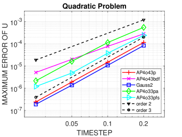
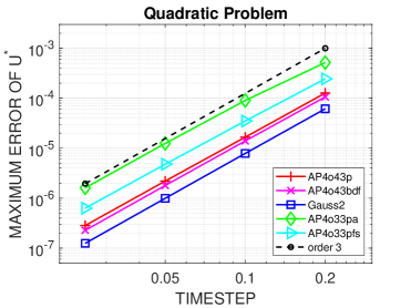
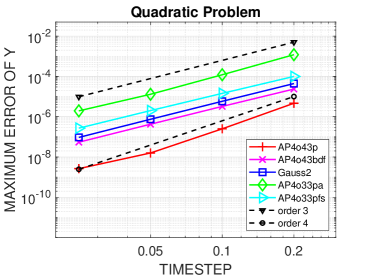
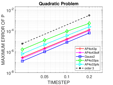
Figure 1: Quadratic Problem. Convergence of the maximal control errors $\|U_{ni}-u(t_{ni})\|_{\infty}$ (top left), improved control errors $\|U^{\star}_{ni}-u(t_{ni})\|_{\infty}$ (top right), state errors $\|Y_{ni,1}-y_{1}(t_{ni})\|_{\infty}$ (bottom left), and adjoint errors $\|P_{ni,1}-p_{1}(t_{ni})\|_{\infty}$, (bottom right), $n=0,\ldots,N,\;i=1,\ldots,s$.

Numerical results for $N\!+\!1\!=\!5,10,20,40$ are shown in Figure 1. All Peer methods show their theoretical order three for the first component of the adjoint variables, $P_{ni,1}$. The fourth-order Gauss-2 method drops down to order three due to its lower stage order three. Order three is also observed for the state variables $Y_{ni,1}$, except for AP4o43p which achieves its super-convergence order four for the first three runs. For the Peer methods, the errors of the control vector $U$ as well as the improved control $U^{\star}$ obtained from the post-processing in (26) decrease with order three as expected. Since AP4o43bdf satisfies the consistency conditions (36) for $u$ with $q\!=\!2$ only, its order in $U$ is two, which is nicely seen. However, the third-order approximations in the first components of $(Y,P)$ yields order three for $U^{\star}$ again. Both methods, AP4o33pa and AP4o33pfs, fall behind the other ones in terms of accuracy. This is not surprising since their better stability properties and the dense output feature of the latter one come with larger error constants.

8.2 Boundary control of an 1D discrete heat equation

The second problem is taken from [18]. It was especially designed to provide exact formulas for analytic solutions of an optimal boundary control problem governed by a one-dimensional discrete heat equation and an objective function that measures the distance of the final state from the target and the control costs. Since no spatial discretization errors are present, numerical orders of time integrators can be observed with high accuracy without computing reference solutions.

The optimal control problem reads as follows:

minimize $$\,\frac{1}{2}\|y(1)-\hat{y}\|^{2}_{2}+\frac{1}{2}\int_{0}^{1}u(t)^{2}\,dt$$

subject to $$\,y^{\prime}(t)=Ay(t)+\gamma e_{m}u(t),\quad t\in(0,1],$$

$$\,y(0)=\mbox{{1\hskip-2.40005ptl}},$$

with

$$A= \frac{1}{(\triangle x)^{2}}\begin{pmatrix}-1&1\\ 1&-2&1\\ &&\ddots&\ddots&\ddots\\ &&&1&-2&1\\ &&&&1&-3\end{pmatrix},$$

state vector $y(t)\in{\mathbb{R}}^{m}$, $\triangle x=1/m$, and $\gamma=2/(\triangle x)^{2}$. The components $y_{i}(t)$ approximate the solution of the continuous 1D heat equation $Y(x,t)$ over the spatial domain $[0,1]$ at the discrete points $x_{i}=(i-0.5)\triangle x$, $i=1,\ldots,m$. The corresponding boundary conditions are $\partial_{x}Y(0,t)=0$ and $Y(1,t)=u(t)$. The matrix $A\in{\mathbb{R}}^{m,m}$ results from standard central finite differences. Its eigenvalues $\lambda_{k}$ and corresponding normalized orthogonal eigenvectors $v^{[k]}$ are given by

$$\lambda_{k}= \;-4m^{2}\sin^{2}\left(\frac{\omega_{k}}{2m}\right),\;\omega_{k}=\left(k-\frac{1}{2}\right)\pi,$$

$$v^{[k]}_{i}= \;\nu_{k}\cos\left(\omega_{k}\frac{2i-1}{2m}\right),\;\nu_{k}=\frac{2}{\sqrt{2m+\sin(2\omega_{k})/\sin(\omega_{k}/m)}},\;\;i,k=1,\ldots,m.$$

We follow the test case in [18] and prescribe the sparse control

$$u(t)=-\gamma p_{m}(t),\quad p(t)= \;\delta\left(e^{\lambda_{1}(T-t)}v^{[1]}+e^{\lambda_{2}(T-t)}v^{[2]}\right),$$

with $\delta=1/75$, which defines the target vector $\hat{y}$ through

$$\hat{y}(t)= \,y(T)-\delta\left(v^{[1]}+v^{[2]}\right).$$

The coefficients $\eta_{k}(T)$ of $y(T)=\sum_{i=1,\ldots,m}\eta_{k}(T)v^{[k]}$ are given by

$$\eta_{k}(T)= \;e^{\lambda_{k}T}\eta_{k}(0)-\gamma^{2}\delta Tv_{m}^{[k]}\sum_{l=1}^{2}v_{m}^{[l]}\varphi_{1}((\lambda_{k}+\lambda_{l})T)$$

where $\eta_{k}(0)=y(0)^{\sf T}v^{[k]}$ and $\varphi_{1}(z):=(e^{z}-1)/z$. We will compare the numerical errors for $y(T)$, $p(0)$ and $u(t)$ An approximation $p_{h}(0)$ for the Peer method is obtained from $p_{h}(0)=(v^{\sf T}\otimes I)P_{0}$ with $v=V_{s}^{-T}e_{s}$, $e_{s}=(0,\ldots,0,1)^{\sf T}\in{\mathbb{R}}^{s}$. Note that, compared to [18], we have changed the sign of the adjoint variables, i.e., $p\mapsto-p$, to fit into our setting. Introducing an additional component $y_{m+1}(t)$ and adding the equations $y^{\prime}_{m+1}(t)=u(t)^{2}$, $y_{m+1}(0)=0$, the objective function can be transformed to the Mayer form

$${\cal C}(y(1)):=\frac{1}{2}\,\left(\sum_{i=1}^{m}(y_{i}(1)-\hat{y}_{i})^{2}+y_{m+1}(1)\right)$$

with the extended vector $y(1)=(y_{1}(1),\ldots,y_{m}(1),y_{m+1}(1))^{\sf T}$. We set $m=500$. In Fig. 2, the analytic control $u(t)$ and the target function $\hat{y}\in{\mathbb{R}}^{m}$ are shown.

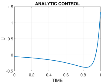
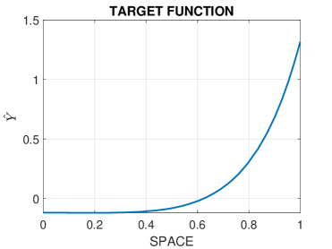
Figure 2: Dirichlet heat problem with $m=500$ spatial points. Analytic control $u(t)$ (left) and target function $\hat{y}$ (right).

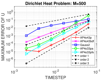
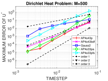
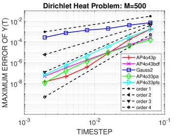
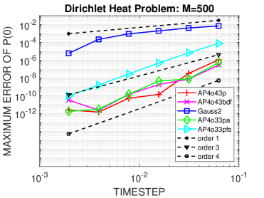
Figure 3: Dirichlet heat problem with $m=500$ spatial points. Convergence of the maximal control errors $\|U_{ni}-u(t_{ni})\|_{\infty}$ (top left), improved control errors $\|U^{\star}_{ni}-u(t_{ni})\|_{\infty}$ (top right), state errors $\|y(T)$$-$$y_{h}(T)\|_{\infty}$ (bottom left), and adjoint errors $\|p(0)$$-$$p_{h}(0)\|_{\infty}$ (bottom right).

We will now discuss the numerical errors obtained from applying $N+1=2^{k}$, $k=4,\ldots,9$, time steps. The results are visualized in Fig. 3. As already observed in [18], the one-step Gauss method of order four suffers from a serious order reduction to first order in all variables $(y,p,u)$. This phenomenon is well understood and occurs particularly drastically for time-dependent Dirichlet boundary conditions [23]. This drawback is shared by all one-step methods due to their insufficient stage order. The BDF-based AP4o43bdf shows second order convergence in the control, which is in accordance with the fact that it satisfies (36) with $q\!=\!2$ only. This also limits the accuracy of the state and the adjoint at their endpoints to order three and two, respectively. Thus, the improvement in the post-processed control variables $U^{*}_{ni}$ is only marginal and does not increase the order. All new Peer methods satisfy (36) for $q\!=\!3$ and deliver approximations of the control with order three, except for certain irregularities in the smallest step. The order of convergence for $y_{h}(T)$ is three for AP4o33pa and AP4o33pfs, whereas AP4o43p reaches fourth-order super-convergence for nearly all time steps. For $p_{h}(0)$, AP4o33pfs shows an ideal order three. The other two Peer methods vary between order three and five and stagnate at the end when errors are already quite small. The supposed improvement in $U^{*}_{ni}$ is not achieved for the Peer methods. Quite to the contrary, AP4o33pf loses two orders of magnitude in accuracy, AP4o43p loses one order. We infer that for Peer methods, which perform close to their theoretical order, the approximation quality of $U$ is nearly optimal and post-processing is not advisable in general. To summarize, the newly constructed Peer methods significantly improve the approximation of the control with increased order three. AP4o43p gains from its super-convergence property and performs remarkably well for this discrete heat problem.

8.3 Stopping of a nucleation process with distributed control

In our third study, we consider a PDE-constrained optimal control problem from [6, Chapter 5.4] – stopping of a nucleation process modelled by a nonlinear reaction-diffusion equation of Schlögl-type. It reads

$$\mbox{minimize }J:= \,\frac{1}{2}\int_{Q}(Y(x,t)-Y_{Q}(x,t))^{2}\,dxdt+\frac{\alpha}{2}\int_{Q}U(x,t)^{2}\,dxdt$$

$$\mbox{subject to }\hskip 14.22636pt\partial_{t}Y-\partial_{xx}Y= \,Y-kY^{3}+U(x,t),\quad(x,t)\in Q:=(0,L)\times(0,T],$$

$$Y(x,0)= \,Y_{0}(x),\quad x\in(0,L),$$

$$\partial_{x}Y(0,t)= \,\partial_{x}Y(L,t)=0,$$

with parameters $\alpha\!=\!10^{-6}$, $L\!=\!20$, $T\!=\!5$, and $k=1/3$. The initial condition is

$$Y_{0}(x)= \,\left\{\begin{array}[]{ll}1.2\,\sqrt{3},&\,x\in[9,11],\\[2.84526pt] 0,&\,\mbox{else}.\end{array}\right.$$

The solution $Y_{nat}(x,t)$ for $U(x,t)\equiv 0$ describes a natural nucleation process with wavelike dispersion to the left and right. The distributed control $U(x,t)$ should now be chosen in such a way that the dispersion is stopped at $t=2.5$, forcing a stationary profile $Y_{nat}(x,2.5)$ for the remaining time interval. Therefore, we set

$$Y_{Q}(x,t)= \,\left\{\begin{array}[]{ll}Y_{nat}(x,t),&\,t\in[0,2.5],\\[2.84526pt] Y_{nat}(x,2.5),&\,t\in(2.5,T],\end{array}\right.$$

in the objective function $J$. There indeed exists an analytic solution for such a control,

$$U_{stop}(x,t)= \,\left\{\begin{array}[]{ll}0,&\,t\leq 2.5,\\[2.84526pt] kY^{3}_{nat}(x,2.5)-Y_{nat}(x,2.5)-\partial_{xx}Y_{nat}(x,2.5),&\,t>2.5,\end{array}\right.$$

since $\partial_{t}Y(x,t)$ must vanish for $t\geq 2.5$. The authors of [6] proved that the second derivative $\partial_{xx}Y_{nat}(x,2.5)$ is well defined. The functions $Y_{nat}$, $Y_{Q}$, and $U_{stop}$ are plotted in Fig. 4.

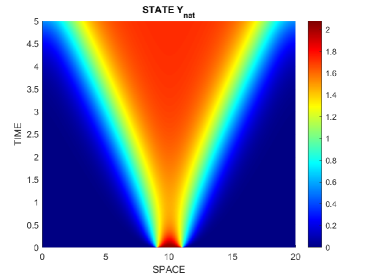
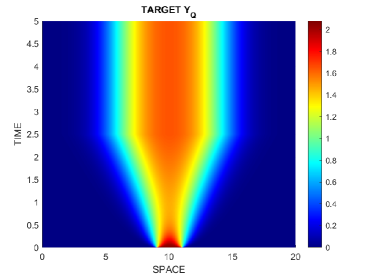
Figure 4: Nucleation process. $Y_{nat}$ for $U=0$ (top, left), target function $Y_{Q}$ (top, right) and analytic control $U_{stop}$ (bottom).

We again use standard finite differences on the shifted spatial mesh $x_{i}=(i-0.5)\triangle x$, $i=1,\ldots,m$, with $\triangle x=L/m$ to discretize the PDE in space. The objective function is approximated by a linear spline. This yields, after transforming to the Mayer form, the discrete control problem

$$\mbox{minimize }{\cal C}\big{(}y(T)\big{)}=y_{m+1}(T)$$

$$\mbox{subject to }y^{\prime}(t)= \,Ay(t)+G(y(t),u(t))=:f(y(t),u(t)),\quad t\in(0,T],$$

$$y(0)= \,\begin{pmatrix}(Y_{0}(x_{i}))_{i=1}^{m}\\[2.84526pt] 0\end{pmatrix},$$

with

$$(G(y,u))_{i}=\left\{\begin{array}[]{ll}-ky_{i}^{3}+y_{i}+u_{i},&\,i=1,\ldots,m,\\[2.84526pt] \displaystyle\frac{1}{2}((y-y_{Q})_{i=1}^{m})^{\sf T}M(y-y_{Q})_{i=1}^{m}+\frac{\alpha}{2}u^{T}Mu,&\,i=m+1,\end{array}\right.$$

and the matrices

$$A=\frac{1}{(\triangle x)^{2}}\begin{pmatrix}-1&1&&&&\\ 1&-2&1&&&\\ &&\ddots&&&\\ &&1&-2&1&\\ &&&1&-1&\\ &&&&&0\end{pmatrix},\quad M=\frac{\triangle x}{12}\begin{pmatrix}10&2&&&\\ 2&8&2&&\\ &&\ddots&&\\ &&2&8&2\\ &&&2&10\\ \end{pmatrix}.$$

Here, $A\in{\mathbb{R}}^{m+1,m+1}$, $M\in{\mathbb{R}}^{m,m}$, $u(t)=(U(x_{i},t))_{i=1}^{m}$, $y_{Q}(t)=((Y_{Q}(x_{i},t)_{i=1}^{m})$ and $y(t)\approx(Y(x_{i},t))_{i=1}^{m+1}$. The total dimension of the discrete control vectors $(U_{nj})$, $n=0,\ldots,N$, $j=1,\ldots,s$, is $ms(N+1)$. We set $m\!=\!300$ as in [6] and note that $s\!=\!4$ for our Peer methods. The optimal stopping control $U_{stop}$ is discretized by

$$u_{stop}(t)= \;\left\{\begin{array}[]{ll}0,&\,t\leq 2.5,\\[2.84526pt] ky_{Q}^{3}(2.5)-y_{Q}(2.5)-\hat{A}y_{Q}(2.5),&\,t>2.5,\end{array}\right.$$

where $\hat{A}=(A)_{i,j=1}^{m}$. With grid sizes $N\in[24,399]$ in time the excessive demand of memory for the full Hessian of the objective function prohibits its use in Matlab’s fmincon subroutine. However, a closer inspection reveals that

$$\nabla_{U_{nj}U_{nj}}{\cal C}=h\alpha\sum_{i=1}^{s}\kappa_{ij}^{[n]}(P_{ni})_{m+1}M\in{\mathbb{R}}^{m,m},\quad n=0,\ldots,N,\;j=1,\ldots,s,$$

are the only entries yielding a sparse tridiagonal Hessian, see Example 7.1. Furthermore, controls $U_{nj}$ with $\kappa_{ij}^{[n]}=0$ for $i=1,\ldots,s,$ are discarded as noted in Chapter 7. Hence, we pass the sparse Hessian to fmincon and switch to the trust-region-reflective algorithm, which allows a simple way for its allocation.

Let us now present the results for the stopping problem and compare them to those documented in [6]. There, the implicit Euler scheme with $h=1/80$, i.e., $400$ uniform time steps, has been applied, together with a nonlinear cg method and different step size rules. Using the optimal control $u_{stop}(t)$ given above in a forward simulation of the ODE, they found ${\cal C}=3.4814\cdot 10^{-6}$ as reference value. This nicely compares to our value ${\cal C}=3.1651\cdot 10^{-6}$ for AP4o43p applied with the same time steps. In principle, the optimizer should find a solution close to it when started with $U^{(0)}=u_{stop}$ evaluated at the time points $t_{n}+c_{i}h$. Computation times and values of the objective function are collected in Table 4. Remarkably, already for $N+1=50$ all Peer methods deliver excellent approximations in very short time compared to $70-100$ seconds reported in [6] for similar calculations. This is a clear advantage of higher-order methods.

N+1	400	200	100	50
AP4o43p	2.99e-6	3.24e-6	3.91e-6	6.02e-6
CPU time [s]	176	51	17	7
AP4o33pa	3.76e-6	6.49e-6	8.12e-6	1.53e-5
CPU time [s]	163	56	27	16
AP4o33pfs	4.17e-6	5.82e-6	1.10e-5	2.62e-5
CPU time [s]	126	72	30	17

Table 4: Values of the objective function ${\cal C}$ and computing times for $U^{(0)}=u_{stop}$ and $N+1=400,200,100,50$ uniform time steps. The reference value is ${\cal C}=3.1651\cdot 10^{-6}$.

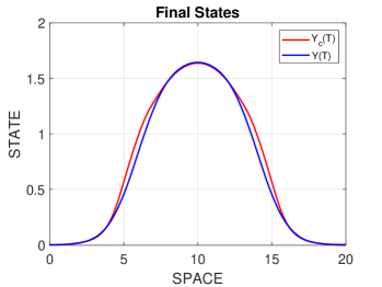
Figure 5: Nucleation process with box constraints for the control. Computed constrained control $U_{c}(t)$ (top left), state $Y_{h}(t)$ (top right), constraint and unconstraint controls at final time $t=T$ (bottom left), and corresponding final states (bottom right) approximated by AP4o43p with $50$ uniform time steps.

Choosing $U^{(0)}=\beta\,u_{stop}$ with $\beta=0.99$, the authors of [6] already discovered slow convergence and tiny deviations from $u_{stop}$ in the shape of the computed optimal control, which were clearly visible in their plots. In contrast, all controls computed by the Peer methods stay close to the overall picture shown in Figure 4 even for $\beta=0.95,0.50$, and for $50$ times steps. The maximal pointwise control errors range around $6\cdot 10^{-3}$ and $5\cdot 10^{-2}$, respectively.

As a last (speculative) test we impose box constraints of the form

$$u(t)\in U_{ad}:=\{u(t)\in[L^{\infty}(0,T)]^{m}|\,-0.5\leq u_{i}(t)\leq 0,\;i=1,\ldots,m,\;t\in(0,T)\}.$$

Now the explicitly given optimal control $U_{stop}$ violates the prescribed bounds with its minimum value $-0.638$. We apply AP4o43p with $50$ uniform time steps and set $U^{(0)}=u_{stop}$. fmincon first restricts the control vector to the admissible set $U_{ad}$ and after $66$ seconds and 142 iteration steps it delivers a solution with ${\cal C}=0.0323$. The stopping process is still quite satisfactory. Details are plotted in Figure 5. We get nearly the same solution for 400 uniform time steps. Interestingly, the restricted analytic optimal control $\hat{u}_{stop}\in U_{ad}$ only yields ${\cal C}=0.0850$, which is larger than that of the Peer solution by a factor of $2.6$.

9 Summary

We have upgraded our four-stage implicit Peer triplets constructed in [17] to meet the additional order conditions and positivity requirements for an efficient use in a gradient-based iterative solution algorithm for ODE constrained optimal control problems. Using super-convergence for both the state and adjoint variables, an $A(59.78^{o})$-stable method AP4o43p of the higher order pair $(4,3)$ was constructed. Lowering the order for the forward scheme, an almost A-stable method AP4o33pa of order pair $(3,3)$ with stability angle $\alpha=89.90^{o}$ could be found. We also considered the class of FSAL methods, where the last stage of the previous time step equals the first stage of the new step, and came up with the $A(77.53^{o})$-stable method AP4o33pfs. A notable theoretical result is that there is no BDF4-based triplet that improves the second-order control approximation of our recently developed AP4o43bdf [17] to the present setting. All methods show their theoretical orders in the numerical experiments and clearly outperform the fourth-order symplectic Runge-Kutta-Gauss method in the boundary control problem for an 1D discrete heat equation proposed in [18] to study order reduction phenomena. The new Peer triplets also perform remarkably well for a PDE-constrained optimal control problem which models the stopping of a nucleation process driven by a reaction-diffusion equation of Schlögl-type. In future work, we will equip our Peer triplets with variable step sizes to further improve their efficiency.

Author Contributions: Conceptualization, J.L. and B.A.S.; investigation, J.L. and B.A.S.; software, J.L. and B.A.S. All authors have read and agreed to the published version of the manuscript.

Funding. The first author is supported by the Deutsche Forschungsgemeinschaft (DFG, German Research Foundation) within the collaborative research center TRR154 “Mathematical modeling, simulation and optimisation using the example of gas networks” (Project-ID 239904186, TRR154/3-2022, TP B01).

Conflicts of Interest: The authors declare no conflict of interest.

Appendix

The coefficient matrices which define the Peer triplets AP4o43p, AP4o33pa and AP4o33pfs discussed above are presented here. We provide exact rational numbers for the node vector ${\bf c}$ and give numbers with $16$ digits for all matrices. It is sufficient to only show pairs $(A_{n},K_{n})$ and the node vector ${\bf c}=(c_{1},\ldots,c_{s})^{\sf T}$ for AP4o43p and some additional data for AP4o33pa and AP4o33pfs, since all other parameters can be easily computed from the following relations:

$$B_{n}= \,(A_{n}V_{4}-K_{n}V_{4}\tilde{E}_{4}+R_{n})P_{4}V_{4}^{-1},\;a=A_{0}\mbox{1\hskip-2.40005ptl},\;w=A_{N}^{\sf T}\mbox{1\hskip-2.40005ptl},\;v=V_{4}^{\sf-T}e_{1},$$

with the special matrices

$$V_{4}=\big{(}\mbox{1\hskip-2.40005ptl},{\bf c},{\bf c}^{2},{\bf c}^{3}),\quad{\cal P}_{4}=\Big{(}{j-1\choose i-1}\Big{)}_{i,j=1}^{4},\quad\tilde{E}_{4}=\big{(}i\delta_{i+1,j}\big{)}_{i,j=1}^{4}\,.$$

The matrices $R_{0},R_{N}$ and $R\equiv R_{n}$ for $1\leq n\leq N-1$ are slack variables at order 4, they vanish for method AP4o43p ($R_{n}\equiv 0$) and are provided for AP4o33pa and AP4o33pfs only.

A1: Coefficients of AP4o43p

$${\bf c}^{\sf T}=\left(\frac{4657}{46172},\frac{43}{97},\frac{3991}{6596},\frac{21111803999}{23798723875}\right)$$

$$\displaystyle A_{0}=\begin{pmatrix}7.666666666666667&-7.952380952380952&6.428571428571429&-1.0\\[2.84526pt] -37.64573385789864&46.51465022124085&-35.34733224501487&5.556742966495919\\[2.84526pt] 38.90401308661976&-51.03310294122830&39.84674769118604&-5.987622148721481\\[2.84526pt] -9.132039686863960&14.19615134612322&-13.42624214739033&3.410910572594644\end{pmatrix}$$

$$\displaystyle K_{0}=\begin{pmatrix}0.2201309814534140&-0.001685331083118719&0.03214426130560293&0\\[2.84526pt] 0.1111845986702137&0.4311745541022918&-0.1774967804652712&0\\[2.84526pt] -0.1188243074116737&-0.009945644225626329&0.2279954173163067&0\\[2.84526pt] 0.02777498546842700&0.002324777899894389&-0.04434040826768050&\kappa_{44}^{[0]}\end{pmatrix}$$

with $\displaystyle\kappa_{44}^{[0]}=0.2883852220354272$.

$$\displaystyle A=\begin{pmatrix}2.080437513028435&0&0&0\\[2.84526pt] -6.582767809460944&2.843481487726957&0&0\\[2.84526pt] 5.640064091163237&-4.381563545251576&2.010790683327275&0\\[2.84526pt] -1.344827586206897&3.263399731279439&-4.509045955975008&1.980031390369082\end{pmatrix}$$

$$\displaystyle K=\,\mbox{diag}\left(0.2523093948412364,0.4504313304404388,0.0,0.2972592747183247\right)$$

$$\displaystyle A_{N}=\begin{pmatrix}2.602941176470588&0.09421300555614037&-1.072906715212599&0.6\\[2.84526pt] -9.770538838886514&3.643517491998914&4.765969638829557&-3.172336041397070\\[2.84526pt] 9.121758438719117&-5.324324324324324&-3.193548387096774&3.514071174094508\\[2.84526pt] -2.137018032260198&3.217404548657921&-2.956254337680976&1.067051202531710\end{pmatrix}$$

$$\displaystyle K_{N}=\begin{pmatrix}0.2752122060365109&0&0.03076923076923077&0.06493506493506494\\[2.84526pt] -0.07088680624623493&\kappa_{22}^{[N]}&-0.1699040256986543&-0.3585636905978095\\[2.84526pt] 0.07575757575757576&0&0.2750926288014159&0.3832012950339724\\[2.84526pt] -0.01770820812361161&0&-0.04244366487128950&0.1921737961617600\end{pmatrix}$$

with $\displaystyle\kappa_{22}^{[N]}=0.3735422712438619$.

A2: Coefficients of AP4o33pa

$${\bf c}^{\sf T}=\left(\frac{46}{5253},\frac{29}{51},\frac{1723}{2193},\frac{17131}{12189}\right)$$

$$\displaystyle A_{0}=\begin{pmatrix}-1.157765450537458&4.180419822183092&-3.571237514138118&0.4344668789817266\\[2.84526pt] 9.320046415868424&-20.43515251977805&20.53668079758682&-2.660420735071554\\[2.84526pt] -9.502446854904932&18.14294953408145&-17.88837560028214&2.643706254438956\\[2.84526pt] 1.573865446847084&-2.968198110625862&2.201646466132119&0.1498151692184390\end{pmatrix}$$

$$\displaystyle K_{0}=\begin{pmatrix}0.1525423728813559&0.06343283582089552&-0.04424778761061947&0\\[2.84526pt] 0.2455414494142291&0.3479528534959272&0.2643445483279409&0\\[2.84526pt] -0.2389119757586965&0.3687279250113433&-0.2354279614690257&0\\[2.84526pt] 0.03447092342852595&-0.05320115087852647&0.03711064142489613&\kappa_{44}^{[0]}\end{pmatrix}$$

with $\displaystyle\kappa_{44}^{[0]}=0.2479535745634692$.

$$\displaystyle A=\begin{pmatrix}0.7073170731707317&0&0&0\\[2.84526pt] -1.458044769359054&2.011111111111111&0&0\\[2.84526pt] 0.8963499143698150&-3.446643123594083&2.170212765957447&0\\[2.84526pt] 0.08807733909162651&0.3555507383436048&-0.8914986166587666&0.5675675675675676\end{pmatrix}$$

$$\displaystyle K=\,\mbox{diag}\left(0.2240817025504534,0.2911518627633785,0.2558139534883721,0.2289524811977960\right)$$

$$\displaystyle R=\begin{pmatrix}0&0&0&-0.2105994034490964\\[2.84526pt] 0&0&0&0.1876445792137739\\[2.84526pt] 0&0&0&-0.1297946665997080\\[2.84526pt] 0&0&0&0.1527494908350306\end{pmatrix}$$

$$\displaystyle A_{N}=\begin{pmatrix}0.03570841538693515&0.4969703797836259&0&0\\[2.84526pt] 2.797947998593283&-2.717111089179658&1.827587054105035&-0.3120359279234260\\[2.84526pt] -3.797058467469895&4.498208855806741&-2.913725127809472&0.8173416699480771\\[2.84526pt] 0.4837073832344139&0.1093148794369315&-0.4021296652058669&0.07527364129327442\end{pmatrix}$$

$$\displaystyle K_{N}=\begin{pmatrix}0.2323465386026342&0.08709000303247828&0&0\\[2.84526pt] 0.0006578497520678987&-0.2800336616814694&0&0\\[2.84526pt] -0.0006400881985255662&0.5062443715754399&0.32694879378132385&0\\[2.84526pt] 0.00009235381026342189&-0.07304242875763006&0&\kappa_{44}^{[N]}\end{pmatrix}$$

with $\displaystyle\kappa_{44}^{[N]}=0.01004801943170234$.

$$\displaystyle R_{N}=\begin{pmatrix}0&0&0&-0.1751101070505921\\[2.84526pt] 0&0&0&0.2296022411517165\\[2.84526pt] 0&0&0&-0.5247365005443616\\[2.84526pt] 0&0&0&-0.07622773831802632\end{pmatrix}$$

A3: Coefficients of AP4o33pfs

$${\bf c}^{\sf T}=\left(0,\frac{9}{86},\frac{321}{602},1\right)$$

$$A_{0}=\begin{pmatrix}1.333333333333333&0&0&0\\[2.84526pt] -2.789814648187671&2.243282202070159&0.06686328023669716&0.01646570267735142\\[2.84526pt] 4.349477807846901&-6.391186028966211&2.276667661951199&-0.06058221663260115\\[2.84526pt] -6.567438826613935&9.406667237260441&-4.671899050533916&1.788163545558252\end{pmatrix}$$

$$K_{0}=\,\mbox{diag}\left(0,0.2868808051464541,0.4845433642003949,0.2814200916147642\right)$$

$$A=\begin{pmatrix}0.7857142857142857&0&0&0\\[2.84526pt] -2.028837530067695&2.203900659027200&0&0\\[2.84526pt] 4.063000939519495&-6.340099591541239&2.287165301103365&0\\[2.84526pt] -6.494320028787459&9.394962342878431&-4.615533409449387&1.744047031603003\end{pmatrix}$$

$$K=\,\mbox{diag}\left(0,0.2754665812532002,0.4295774647887324,0.2949559539580673\right)$$

$$R=\begin{pmatrix}0&0&0&0\\[2.84526pt] 0&0&0&0.156340095159149050\\[2.84526pt] 0&0&0&-0.0212049600240154176\\[2.84526pt] 0&0&0&-0.135135135135135135\end{pmatrix}$$

$$A_{N}=\begin{pmatrix}1&0&0&0\\[2.84526pt] -1.037159659693408&0.4363577782952090&0.6845553714934806&-0.2064640160522880\\[2.84526pt] 0.03605110452225963&-0.5660510638564654&-0.1074762596776216&0.7596425122215622\\[2.84526pt] 0.001108555171148741&0.1296932855612564&-0.5770791118158589&0.4468215038307258\end{pmatrix}$$

$$K_{N}=\begin{pmatrix}0.3333333333333333&0&0&0\\[2.84526pt] -0.3406285072951739&0.1264725806602174&0&0\\[2.84526pt] 0.1282327493289677&0&0.5627483658896584&0\\[2.84526pt] -0.03272942952658255&0&0&0.1697266466479663\end{pmatrix}$$

$$R_{N}=\begin{pmatrix}0&0&0&0.0463093438915248733\\[2.84526pt] 0&0&0&0.191797796516481359\\[2.84526pt] 0&0&0&-0.286597642859776972\\[2.84526pt] 0&0&0&0.1785714285714285754\\[2.84526pt] \end{pmatrix}$$

References

- [1] G. Albi, M. Herty, and L. Pareschi. Linear multistep methods for optimal control problems and applications to hyperbolic relaxation systems. Appl. Math. Comput., 354:460–477, 2019.
- [2] I. Almuslimani and G. Vilmart. Explicit stabilized integrators for stiff optimal control problems. SIAM J. Sci. Comput., 43:A721–A743, 2021.
- [3] S. Beck, R. Weiner, H. Podhaisky, and B.A. Schmitt. Implicit peer methods for large stiff ODE systems. J. Appl. Math. Comput., 38:389–406, 2012.
- [4] D. Beigel, M.S. Mommer, L. Wirsching, and H.G. Bock. Approximation of weak adjoints by reverse automatic differentiation of BDF methods. Numer. Math., 126:383–412, 2014.
- [5] F.J. Bonnans and J. Laurent-Varin. Computation of order conditions for symplectic partitioned Runge-Kutta schemes with application to optimal control. Numer. Math., 103:1–10, 2006.
- [6] R. Buchholz, H. Engel, E. Kammann, and F. Tröltzsch. On the optimal control of the Schlögl-model. Comput. Optim. Appl., 56:153–185, 2013.
- [7] R.H. Byrd, J.C. Gilbert, and J. Nocedal. A trust region method based on interior point techniques for nonlinear programming. Math. Program., 89:149–185, 2000.
- [8] T.F. Coleman and Y. Li. On the convergence of reflective Newton methods for large-scale nonlinear minimization subject to bounds. Math. Program., 67:189–224, 1994.
- [9] A. Gerisch, J. Lang, H. Podhaisky, and R. Weiner. High-order linearly implicit two-step peer – finite element methods for time-dependent PDEs. Appl. Numer. Math., 59:624–638, 2009.
- [10] W.W. Hager. Rate of convergence for discrete approximations to unconstrained control problems. SIAM J. Numer. Anal., 13:449–471, 1976.
- [11] W.W. Hager. Runge-Kutta methods in optimal control and the transformed adjoint system. Numer. Math., 87:247–282, 2000.
- [12] W.W. Hager and R. Rostamian. Optimal coatings, bang-bang controls, and gradient techniques. Optim. Control Appl. Meth., 8:1–20, 1987.
- [13] E. Hairer, G. Wanner, and Ch. Lubich. Geometric Numerical Integration, Structure-Preserving Algorithms for Ordinary Differential Equations, volume 31 of Springer Series in Computational Mathematic. Springer, Heidelberg, Berlin, 1970.
- [14] M. Herty, L. Pareschi, and S. Steffensen. Implicit-explicit Runge-Kutta schemes for numerical discretization of optimal control problems. SIAM J. Numer. Anal., 51:1875–1899, 2013.
- [15] S. Jebens, O. Knoth, and R. Weiner. Explicit two-step peer methods for the compressible Euler equations. Mon. Wea. Rev., 137:2380–2392, 2009.
- [16] J. Lang and B.A. Schmitt. Discrete adjoint implicit peer methods in optimal control. J. Comput. Appl. Math., 416:114596, 2022.
- [17] J. Lang and B.A. Schmitt. Implicit A-stable peer triplets for ODE constrained optimal control problems. Algorithms, 15:310, 2022.
- [18] J. Lang and B.A. Schmitt. Exact discrete solutions of boundary control problems for the 1D heat equation. J. Optim. Theory Appl., 2023.
- [19] J. Lang and J.G. Verwer. W-methods in optimal control. Numer. Math., 124:337–360, 2013.
- [20] X. Liu and J. Frank. Symplectic Runge-Kutta discretization of a regularized forward-backward sweep iteration for optimal control problems. J. Comput. Appl. Math., 383:113133, 2021.
- [21] F.C. Massa, G. Noventa, M. Lorini, F. Bassi, and A. Ghidoni. High-order linearly implicit two-step peer methods for the discontinuous Galerkin solution of the incompressible Navier-Stokes equations. Computers & Fluids, 162:55–71, 2018.
- [22] T. Matsuda and Y. Miyatake. Generalization of partitioned Runge–Kutta methods for adjoint systems. J. Comput. Appl. Math., 388:113308, 2021.
- [23] A. Ostermann and M. Roche. Runge-Kutta methods for partial differential equations and fractional orders of convergence. Math. Comp., 59:403–420, 1992.
- [24] H. Podhaisky, R. Weiner, and B.A. Schmitt. Rosenbrock-type ’Peer’ two-step methods. Appl. Numer. Math., 53:409–420, 2005.
- [25] J.M. Sanz-Serna. Symplectic Runge–Kutta schemes for adjoint equations, automatic differentiation, optimal control, and more. SIAM Review, 58:3–33, 2016.
- [26] B.A. Schmitt and R. Weiner. Parallel two-step W-methods with peer variables. SIAM J. Numer. Anal., 42(1):265–282, 2004.
- [27] B.A. Schmitt, R. Weiner, and S. Beck. Two-step peer methods with continuous output. BIT, 53:717–739, 2013.
- [28] M. Schneider, J. Lang, and R. Weiner. Super-convergent implicit-explicit Peer methods with variable step sizes. J. Comput. Appl. Math., page 112501, 2021.
- [29] D. Schröder, J. Lang, and R. Weiner. Stability and consistency of discrete adjoint implicit peer methods. J. Comput. Appl. Math., 262:73–86, 2014.
- [30] J.L. Troutman. Variational Calculus and Optimal Control. Springer, New York, 1996.