Symmetry Groupoids for Pattern-Selective Feedback Stabilization of the Chafee–Infante Equation

Abstract

Reaction-diffusion equations are ubiquitous in various scientific domains and their patterns represent a fascinating area of investigation. However, many of these patterns are unstable and therefore challenging to observe. To overcome this limitation, we present new noninvasive feedback controls based on symmetry groupoids. As a concrete example, we employ these controls to selectively stabilize unstable equilibria of the Chafee–Infante equation under Dirichlet boundary conditions on the interval. Unlike conventional reflection-based control schemes, our approach incorporates additional symmetries that enable us to design new convolution controls for stabilization. By demonstrating the efficacy of our method, we provide a new tool for investigating and controlling systems with unstable patterns, with potential implications for a wide range of scientific disciplines.

Based on a Fourier basis, we characterize dynamically invariant subspaces and introduce convolution controls guided by symmetry groupoids. Our research highlights the effectiveness of symmetry groupoids in characterizing spatio-temporal symmetries of patterns and their potential to facilitate pattern-selective feedback stabilization.

I Introduction

Natural phenomena such as branching in plants Meinhardt, Koch, and Bernasconi (1998), leopard spots Murray (1988), and sea shell Meinhardt (1995); as well as artificial phenomena like rotating spirals in the Belousov–Zhabotinsky reaction Winfree (1984); Zhabotinsky (1991) all exhibit spatio-temporally ordered structures known as patterns. Moreover, pattern formation is also observed in other fields, including fluid dynamics Rand (1982); Crawford and Knobloch (1991), solid-state physics Hoyle (2006), and nonlinear optics Lu, Yu, and Harrison (1996). The diffusion-induced Turing instability reveals a universal mechanism for pattern formation Turing (1952), making models in the form of reaction-diffusion partial differential equations (abbr. PDEs) highly suitable for describing and predicting a wide range of patterns Fiedler and Scheel (2003); Murray (2003).

From a mathematical perspective, a pattern can be defined as a representation of a solution to the underlying PDEs Golubitsky and Stewart (2003). However, when the solution is unstable, it becomes vulnerable to errors in experimental or numerical simulations, resulting in a pattern that is rarely observable. Therefore, the control of unstable patterns has been studied extensively, both theoretically and in diverse applied contexts such as optics, lasers, or control of cardiac tissue Hövel and Schöll (2005); Jensen, Schwab, and Denz (1998); Kyrychko et al. (2009); Lehnert et al. (2011); Ott, Grebogi, and Yorke (1990); Rappel, Fenton, and Karma (1999); Schikora et al. (2006); Yanchuk et al. (2006).

In this article, we explore a novel method to stabilize unstable solutions through the use of noninvasive feedback controls. More specifically, we introduce the concept of convolution controls, which extends both the Pyragas control for ordinary differential equations (abbr. ODEs) Pyragas (1992) and the symmetry-breaking controls for PDEs Schneider (2016); Schneider, de Wolff, and Dai (2022). The specifics of convolution controls will be defined in the following sections. As a concrete application, we design convolution controls and exploit them to stabilize unstable equilibria (i.e., time-independent solutions) of the Chafee–Infante equation Chafee and Infante (1974),

$$\partial_{t}u=u_{xx}+\lambda u(1-u^{2}),$$ (1)

on the interval $x\in(0,\pi)$ equipped with Dirichlet boundary conditions

$$u(t,0)=u(t,\pi)=0\quad\mbox{for }\,t\geq 0.$$ (2)

Here $\lambda>0$ is a bifurcation parameter, which can be regarded as a scale on the length of the interval. Extensive research has been carried out on the Chafee–Infante equationHenry (1981); Fiedler and Rocha (1996); Fiedler and Scheel (2003), and it is nowadays considered as a prototype for reaction-diffusion equations.

Our control strategy is motivated by the Pyragas control method, which is used to stabilize equilibria or periodic solutions of ODEs of the form $\dot{q}(t)=f(q(t))$, where $q(t)\in\mathbb{R}^{n}$. The Pyragas control method employs the following control system with time-delayed feedback:

$$\dot{q}(t)=f(q(t))+b(q(t)-q(t-\tau)).$$ (3)

Here $\tau\geq 0$ is a prescribed time delay and $b\in\mathbb{R}^{n\times n}$ is called the feedback gain matrix. The Pyragas control term

$$b(q(t)-q(t-\tau))$$ (4)

is noninvasive because it vanishes on equilibria and on any $\tau$-periodic solutions, while it possibly changes the local stability property of the targeted solution for a suitably chosen feedback gain $b$. The Pyragas control scheme is widely applicable because it it model independent and inexpensive to implement Pyragas (2006); Schikora et al. (2006); Yamasue et al. (2009). Various generalizations of the Pyragas control, in the setting of ODEs, have been established Nakajima and Ueda (1998); Socolar, Sukow, and Gauthier (1994); Kittel, Parisi, and Pyragas (1995); Schneider and Bosewitz (2016).

Motivated by the observation that symmetry-breaking bifurcations often trigger pattern formation in PDEs Golubitsky and Stewart (2003); Hoyle (2006), Schneider extended the Pyragas control method to include symmetry-breaking controls Schneider (2016). These controls are designed by considering the spatio-temporal symmetries of the targeted solution rather than the full equivariance of the uncontrolled system. To illustrate this concept regarding controls, we consider the Chafee–Infante equation (1)–(2). The symmetry-breaking control system reads

$$\partial_{t}u=u_{xx}+\lambda u(1-u^{2})+b(u-(\pm 1)u(t-\tau,\pi-x)),$$ (5)

where $u=u(t,x)$. The symmetry-breaking control term

$$b(u-(\pm 1)u(t-\tau,\pi-x))$$ (6)

includes a multiplicative factor $\pm 1$, a time delay $\tau\geq 0$, and a space reflection $x\mapsto\pi-x$. Hence it distinguishes between even-symmetric solutions (i.e., $u(t,\pi-x)=u(t,x)$) and odd-symmetric solutions (i.e., $u(t,\pi-x)=-u(t,x)$) with respect to $x=\frac{\pi}{2}$, but it does not distinguish other solutions. A theoretical limitation arises as a result, where symmetry-breaking controls are generally unable to stabilize all equilibria possessing the same reflection symmetry. In particular, it is impossible to select a specific equilibrium to be stabilizedSchneider (2016); see Figure 1 for an illustration of two equilibria that possess the same reflection symmetry with respect to $x=\frac{\pi}{2}$.

In order to selectively stabilize all unstable solutions, our article goes beyond the classical characterization of spatio-temporal symmetries of the targeted solution and proposes the design of more general control terms.

Our control design is motivated by the sifting property of the Dirac delta functional $\delta$, which can be expressed as

$$u(t,x)=(\delta\ast u)(t,x)=\int_{0}^{\pi}\delta(x-\xi)u(t,\xi)\,\mathrm{d}\xi,$$ (7)

where $\ast$ denotes the standard convolution operation. This property implies that the control term $b(u-\delta\ast u)$ is noninvasive to all functions $u$. However, stabilization is bound to fail when the control term is identically zero. Therefore, it is crucial to identify suitable functionals such that the convolution control term is noninvasive exclusively on the targeted solution, while being invasive on other solutions. This approach ensures that the targeted solution is selected and then stabilized.

It is important to emphasize that convolution controls represent a generalization of symmetry-breaking controls (6), because $u(t-\tau,\pi-x)=(h\ast u)(t-\tau,x)$ with $h(z):=\delta(\pi-z)$.

Based on the Fourier basis associated with Dirichlet boundary conditions (2) in Section III and a straightforward calculation in Section IV, we propose the following convolution control system:

$$\partial_{t}u =u_{xx}+\lambda u(1-u^{2})+b(u-\mathcal{C}_{(h,\tau)}[u]),$$ (8)

where the convolution control operator takes the form

$$\mathcal{C}_{(h,\tau)}[u](t,x)=\int_{0}^{\pi}(h(x-\xi)-h(x+\xi))u(t-\tau,\xi)\,\mathrm{d}\xi.$$ (9)

Here $h$ is a kernel functional formally expressed by

$$h(z):=\frac{1}{\pi}\sum_{m=0}^{\infty}h_{m}\cos(mz),\quad z\in\mathbb{R},\,h_{m}\in\mathbb{R}.$$ (10)

The new control scheme will be pattern-selective in the sense that it only preserves the targeted equilibrium.

Our objective is therefore to identify the set $H_{*}$ of kernel functionals $h$ that allow stabilization of an unstable solution $u_{*}$. The key to stabilization lies in the convolution control term

$$b(u-\mathcal{C}_{(h,\tau)}[u]),$$ (11)

which should vanish solely on the targeted solution $u_{*}$, and not on any of the unstable and center eigenfunctions associated with $u_{*}$. Therefore, it is essential to determine dynamically invariant subspaces $X_{*}$ that contain $u_{*}$, as well as to find suitable sets $H_{*}$. Achieving this requires more symmetries beyond equivariance Chossat and Lauterbach (2000); Golubitsky, Schaeffer, and Stewart (1988); Golubitsky and Stewart (2003) of the underlying model.

To demonstrate this requirement, we consider the Chafee-Infante equation (1)–(2). In this case, the only equivariance presented is the space reflection, $x\mapsto\pi-x$, which represents an action of the group $\mathbb{Z}_{2}$. This equivariance only distinguishes solutions that are even-symmetric or odd-symmetric, and it is insufficient to stabilize all solutions with the same reflection symmetry. To overcome this limitation, we turn to the theory of symmetry groupoidsSchneider (2022) that allows us to incorporate additional symmetries that are necessary for stabilization.

The concept of groupoids extends the notion of groups Brown (1987); Ibort and Rodriguez (2019). For the convenience of the reader, the definition of groupoids is given in Appendix Definition. Groupoids serve as a powerful instrument for understanding the symmetrical structure in different fields, such as quantum mechanics Baez and Dolan (2001); Ciaglia, Ibort, and Marmo (2018), string theory Saemann and Szabo (2013), material science Freed and Moore (2013), and general relativity Blohmann, Fernandes, and Weinstein (2013).

From an algebraic perspective, a groupoid is composed of a set of objects, which, in our scenario, correspond to the dynamically invariant spaces $X_{*}$, and a set of morphisms, which in our case, are represented by the kernel functionals that interconnect these objects. Unlike group elements, morphisms in a groupoid may not always have a defined composition, which offers more flexibility and intricacy in the symmetry structure. For the Chafee–Infante equation, groupoids enable us to identify symmetries on a functional level.

The concept of groupoid symmetries (see Appendix Definition) has been developed by Schneider as a tool to characterize symmetries and equivariance in dynamical systems where the group theory may not be suitable Schneider (2022), for instance, when symmetries are non-transitive or when various kinds of symmetries operate on distinct subspaces simultaneously.

This article is organized as follows: Section II provides a brief explanation of the well-known bifurcation structure of Chafee–Infante equilibria. Section III delves into the characterization of dynamically invariant subspaces, referred to as vertex spaces, for any targeted equilibrium. In Section IV, sets of kernel functionals, called vertex isotropy groups, are characterized for stabilization through convolution controls. The proof of stabilization is presented in Section V. Finally, Section VI offers a summary and explores several directions for future research.

To make the article more accessible, we have provided full mathematical details in the appendices. Specifically, Appendix A introduces the functional setting and the notion of stability. Additionally, Appendix B serves as a brief introduction to symmetry groupoids and equivaroid dynamical systems.

II Bifurcation structure of equilibria

To set the stage for our analysis and control in the upcoming sections, we give a concise explanation for the bifurcation structure of Chafee–Infante equilibria. To this end, we introduce the following notation: For each $s\geq 0$, $H_{0}^{s}$ denotes the Sobolev space of the functions $v:[0,\pi]\rightarrow\mathbb{R}$ such that $v(0)=v(\pi)=0$ and the following norm is finite:

$$|v|_{H^{s}}:=\left(\sum_{k=0}^{\infty}(1+k^{2})^{s}|\hat{v}_{k}|^{2}\right)^{\frac{1}{2}}.$$ (12)

Here $\hat{v}_{k}:=\frac{2}{\pi}\int_{0}^{\pi}v(x)\sin(kx)\,\mathrm{d}x$ denotes the $k$-th Fourier coefficient of $v$. The case $s=0$ stands for the Lebesgue space $L^{2}$.

It is known that the Chafee–Infante equation (1)–(2) displays countably many bifurcation curves $\Gamma_{j}$ for $j\in\mathbb{N}$, which emanate from the trivial equilibrium $u=0$. These bifurcation curves are of supercritical pitchfork type; see Ref. Henry (1981) Section 5.3 and Figure 2. Each point $(\lambda,u)$ with $u\neq 0$ on a bifurcation curve corresponds to a nontrivial equilibrium. The curve $\Gamma_{j}$ bifurcates at

$$\lambda_{j}=j^{2}\pi^{2}\quad\mbox{for }j\in\mathbb{N},$$ (13)

corresponding to the $j$-th Dirichlet eigenvalue of the Laplace operator $-\partial_{xx}$ on the interval $[0,\pi]$. The $L^{2}$-normalized eigenfunction associated with $\lambda_{j}$ is $\frac{2}{\pi}\sin(jx)$.

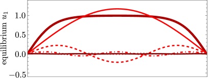
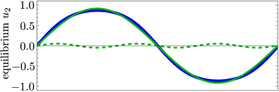
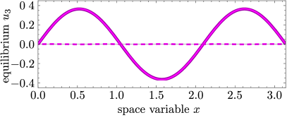
Figure 1: Equilibria of the Chafee–Infante equation (1)–(2) for $\lambda=10$ together with their Fourier expansions for $k\leq 9$. The equilibrium $u_{1}$ (solid dark red curve) lies in the space $X_{1}=\left\{\sum_{\ell\in\mathbb{N}_{odd}}a_{1\ell}\sin(\ell x)\right\}$, that is, it consists of all sine functions (red curves, the curve corresponding to $a_{1}\sin(x)$ is solid, while the other curves are dashed, dot-dashed and dotted, respectively) that are even-symmetric with respect to $x=\frac{\pi}{2}$. In contrast, the equilibrium $u_{2}$ (solid dark blue curve) lying in the space $X_{2}=\left\{\sum_{\ell\in\mathbb{N}_{odd}}a_{2\ell}\sin(2\ell x)\right\}$ is odd-symmetric with respect to $x=\frac{\pi}{2}$ and locally even-symmetric with respect to $x=\frac{\pi}{4},\frac{3\pi}{4}$. It consists of only those sine functions that obey those odd-even symmetries (sine curves in green, the curve corresponding to $a_{2}\sin(2x)$ is solid, while the other curve corresponding to $a_{6}\sin(6x)$ is dashed). Last, the equilibrium $u_{3}$ (solid dark violet curve) is also locally even-symmetric with respect to $x=\frac{\pi}{6},\frac{\pi}{2},\frac{5\pi}{6}$, as well as locally odd-symmetric with respect to $x=\frac{\pi}{3},\frac{2\pi}{3}$. It therefore lies in a smaller subspace $X_{3}=\left\{\sum_{\ell\in\mathbb{N}_{odd}}a_{3\ell}\sin(3\ell x)\right\}$ than $X_{1}$ as compared to the equilibrium $u_{1}$, even though both equilibria would generally be described as “even-symmetric” with respect to $x=\frac{\pi}{2}$. Note that the curve corresponding to $a_{3}\sin(3x)$ (solid magenta curve) lies on the equilibrium $u_{3}$ to a high precision, the curve corresponding to $a_{9}\sin(9x)$ (dashed magenta curve) is almost identical zero.

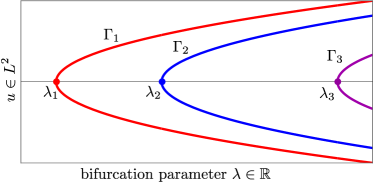
Figure 2: The supercritical pitchfork bifurcation diagram of equilibria for the Chafee–Infante equation (1)–(2). The bifurcation curves are indexed by the unstable dimension $j-1\in\mathbb{N}_{0}$ of equilibria. In particular, all equilibria on $\Gamma_{j}$ for $j\geq 2$ are unstable.

According to the shooting argument used to solve the Sturm–Liouville eigenvalue problems (see Ref. Dai (2021) Lemma 3.3 and Ref. Dai and Lappicy (2021) Theorem 3), every equilibrium $u_{j}(x)$ located on $\Gamma_{j}$ has $j-1$ simple zeros within the interval $(0,\pi)$, and its unstable dimension is also $j-1$. Therefore, all equilibria on $\Gamma_{j}$ with $j\geq 2$ are unstable and provide ideal candidates for stabilization.

Finally, using symmetry arguments from equivariant bifurcation theory (see Ref. Dai (2021) Lemma 3.3), it is well established that for $j\in\mathbb{N}$ and $x\in[0,\pi]$, the relation

$$u_{j}(\pi-x)=(-1)^{j-1}u_{j}(x)$$ (14)

holds, indicating that every equilibrium has a reflection symmetry with respect to $x=\frac{\pi}{2}$.

In the following sections, we will unveil novel properties of the bifurcation curves. Concretely, we prove that these curves lie within distinctive dynamically invariant subspaces that we denote as vertex spaces. Additionally, we will reveal specific actions of so-called vertex isotropy groups that preserve each element of the vertex spaces. These vertex isotropy groups form part of the symmetry groupoid. All of these ingredients are crucial to our design of convolution controls.

III Dynamically invariant vertex spaces

In order to characterize the dynamically invariant linear subspaces and consequently the symmetries of equilibria of the Chafee–Infante equation (1)–(2), we use the orthonormal Fourier basis of $L^{2}$,

$$\left\{\frac{2}{\pi}\sin(kx):k\in\mathbb{N}\right\},$$ (15)

whose elements are the $L^{2}$-normalized eigenfunctions of the Laplace operator $-\partial_{xx}$ with Dirichlet boundary conditions (2). Then, for each fixed $j\in\mathbb{N}$, we define the following $L^{2}$-subspaces, which we call vertex spaces Schneider (2022):

$$X_{j}=\left\{\sum_{\ell\in\mathbb{N}_{odd}}a_{j\ell}\sin(j\ell x)\right\},$$ (16)

where $\mathbb{N}_{odd}$ denotes the set of odd positive integers. See Figure 1 for a visualization of the equilibria lying in their respective vertex spaces.

Remark.

We have the option to choose larger vertex spaces as an alternative, defined as

$$\tilde{X}_{j}=\left\{\sum_{\ell\in\mathbb{N}}\tilde{a}_{j\ell}\sin(j\ell x)\right\}.$$ (17)

In this context, "larger" refers to the inclusion relationship $X_{j}\subset\tilde{X}_{j}$. While both options adequately describe the symmetry of the Chafee–Infante equation (1)–(2), in the context of control, we will observe that it is more advantageous to utilize the smaller vertex spaces $X_{j}$.

The first important property of these vertex spaces $X_{j}$ is that they are dynamically invariant for the Chafee–Infante equation (1)–(2), i.e., the nonlinearity

$$\mathcal{F}(\lambda,u):=u_{xx}+\lambda u(1-u^{2})$$ (18)

maps a dense subspace $Y_{j}\subset X_{j}$ into $X_{j}$. To understand this in a rigorous way, we consider the functional setting $\mathcal{F}:H_{0}^{2}\rightarrow L^{2}$; see Appendix A. Accordingly, we define the $H^{2}$-subspace

$$Y_{j}=X_{j}\Big{|}_{H_{0}^{2}},$$ (19)

i.e., the restriction of $X_{j}$ to $H_{0}^{2}$ equipped with the $H^{2}$-norm. Although the spaces $X_{j}$ and $Y_{j}$ differ by their norms, they consist of the same form for smooth functions and so they are identical from the symmetry perspective.

Lemma 1 (Vertex spaces are dynamically invariant under $\mathcal{F}$).

The nonlinearity $\mathcal{F}(\lambda,u)=u_{xx}+\lambda u(1-u^{2})$ maps $Y_{j}$ into $X_{j}$.

Proof.

Since $\{\sin(kx):k\in\mathbb{N}\}$ is the set of Dirichlet eigenfunctions of $-\partial_{xx}$, it suffices to show that the nonlinear part $u\mapsto u^{3}$ maps $Y_{j}$ into $X_{j}$. The Sobolev embedding theorem guarantees that every function in $H_{0}^{2}$ is continuous. So if $u\in Y_{j}\subset H_{0}^{2}$, then $u$ is continuous, and consequently, $u^{3}\in L^{2}$. Finally, the trigonometric identity

$$4\sin^{3}(\alpha)=3\sin(\alpha)-\sin(3\alpha)\quad\mbox{for }\alpha\in\mathbb{R}$$ (20)

implies $u^{3}\in X_{j}$. ∎

The next important property is that the bifurcation curve $\Gamma_{j}$ is contained in the vertex space $Y_{j}$.

Lemma 2 (Nontrivial equilibria lie in vertex spaces).

Let $u_{j}$ be a nontrivial equilibrium on $\Gamma_{j}$. Then $u_{j}\in Y_{j}$.

Proof.

Since $\mathcal{F}$ maps to $Y_{j}$ into $X_{j}$ by Lemma 1, we can restrict the Chafee–Infante equation (1)–(2) to $Y_{j}$. At the bifurcation point $(\lambda_{j},0)$ of the bifurcation curve $\Gamma_{j}$, the linearized operator (i.e., the partial Fréchet derivative) $\partial_{u}\mathcal{F}(\lambda_{j},0):Y_{j}\rightarrow X_{j}$ defined by

$$\partial_{u}\mathcal{F}(\lambda_{j},0)[v]:=v_{xx}+\lambda_{j}v$$ (21)

has an eigenfunction $\sin(jx)$, which belongs to $Y_{j}$. Since $\lambda_{j}$ is a simple eigenvalue of $-\partial_{xx}$, by the theorem of bifurcation from simple eigenvalues Crandall and Rabinowitz (1971), nontrivial equilibria in $Y_{j}$ that bifurcate from $(\lambda_{j},0)$ exist and form a bifurcation curve $\tilde{\Gamma}_{j}\subset\mathbb{R}\times Y_{j}$. The uniqueness of bifurcation curves from simple eigenvalues implies $\Gamma_{j}=\tilde{\Gamma}_{j}$ and thereby $u_{j}\in Y_{j}$. ∎

Notice that the same result as in Lemma 2 can be achieved by using the equivaroid branching lemma, which is a broader variant of the classical equivariant branching lemmaGolubitsky and Stewart (2003); see Ref. Schneider (2022) for more information.

IV Vertex isotropy groups and convolution controls

We begin by examining a targeted equilibrium $u_{j}$ on $\Gamma_{j}$ and we use the noninvasiveness condition to characterize sets of kernel functionals, which we refer to as vertex isotropy groups. After characterizing these groups, we derive an explicit expression for the convolution control operator.

Recall that the targeted equilibrium $u_{j}$ belongs to the vertex space $Y_{j}$ by Lemma 2. To stabilize $u_{j}$, our first step is to obtain kernel functionals $h$ such that the control term $b(u-\mathcal{C}_{(h,\tau)}[u])$ is noninvasive on $u_{j}$, i.e.,

$$u_{j}-\mathcal{C}_{(h,\tau)}[u_{j}]=0.$$ (22)

Since we aim to stabilize equilibria, the time delay $\tau\geq 0$ is irrelevant to (22). Hence for simplicity we take $\tau=0$ and denote $\mathcal{C}_{h}:=\mathcal{C}_{(h,0)}$.

A sufficient condition for (22) is to choose functionals $h$ such that the control term is noninvasive on all functions in $Y_{j}$. Equivalently, the control operator $\mathcal{C}_{h}$ acts as the identity operator on the targeted vertex space, i.e.,

$$\mathcal{C}_{h}\Big{|}_{Y_{j}}=\mathcal{I}_{j},$$ (23)

where $\mathcal{I}_{j}:Y_{j}\rightarrow X_{j}$, $\mathcal{I}_{j}[v]=v$, is the identity operator.

We collect all candidates to kernel functionals in the following vertex isotropy group: For each fixed $j\in\mathbb{N}$, we define

$$H_{j}:=\left\{\frac{1}{\pi}\sum_{m=1}^{\infty}h_{m}\cos(mz):h_{jm}=1\mbox{ for }m\in\mathbb{N}_{odd}\right\}$$ (24)

and call each $h_{m}$ a control parameter. Notice that $h(z)=\frac{1}{\pi}\sum_{m=1}^{\infty}h_{m}\cos(mz)$ is not a function in any $L^{p}$-space, because $h_{jm}=1$ for $m\in\mathbb{N}_{odd}$. Instead, the infinite series above is a formal expression of the kernel functional $h$.

Remark.

Had we chosen the larger vertex spaces $\tilde{X_{j}}$ defined in (17) rather than $X_{j}$, it would have given us the smaller vertex isotropy groups

$$\tilde{H}_{j}:=\left\{\frac{1}{\pi}\sum_{m=1}^{\infty}\tilde{h}_{m}\cos(mz):\tilde{h}_{jm}=1\mbox{ for }m\in\mathbb{N}\right\},$$ (25)

and so our choice of control parameters would have been limited.

It is important to recognize that the pair $(Y_{j},H_{j})$ constitutes a symmetry groupoid in which the objects correspond to the vertex spaces $Y_{j}$ and the morphisms correspond to the vertex isotropy groups $H_{j}$. Notably, the symmetries within the vertex isotropy groups solely apply to the subspaces $Y_{j}$ and not to the full space $H_{0}^{2}$, rendering the standard group theory not applicable. Moreover, readers may observe that the vertex isotropy groups $H_{j}$ and $\tilde{H}_{j}$ do not contain the complete set of symmetries for the Chafee–Infante equation (1)–(2). The reason is that, for the sake of brevity, we have only included the part of the symmetry groupoid that is relevant to our control scheme. Furthermore, symmetry groupoids have applications in a broader range of contexts. The fundamental concepts and general definitions can be found in Appendix B.

We are now ready to derive an explicit expression for the convolution control operator:

$$\mathcal{C}_{h}[v](x)=\int_{0}^{\pi}(h(x-\xi)-h(x+\xi))v(\xi)\,\mathrm{d}\xi.$$ (26)

Note that this operator also represents the action of the vertex isotropy group $H_{j}$ on the function space $H_{0}^{2}$: Given any kernel functional $h$ formally expressed by $h(z)=\frac{1}{\pi}\sum_{m=1}^{\infty}h_{m}\cos(mz)$, the convolution control operator acts on functions $v(x)=\sum_{k=1}^{\infty}a_{k}\sin(kx)$ in the full space $H_{0}^{2}$. Using the trigonometric identity

$$\cos(\alpha-\beta)-\cos(\alpha+\beta)=2\sin(\alpha)\sin(\beta)\quad\mbox{for }\alpha,\beta\in\mathbb{R},$$ (27)

and noting

$$\int_{0}^{\pi}\sin(m\xi)\sin(k\xi)\,\mathrm{d}\xi=\frac{\pi}{2}\delta_{m,k},$$ (28)

where $\delta_{m,k}$ is the Kronecker delta defined by $\delta_{m,k}=1$ if $m=k$ and $\delta_{m,k}=0$ if $m\neq k$, from (26)–(28) we obtain

$$\mathcal{C}_{h}[v](x)=\sum_{k=1}^{\infty}h_{k}a_{k}\sin(kx).$$ (29)

Indeed, the convolution acts as a termwise multiplication on the Fourier coefficients of the function $v(x)$.

From the formula (29), it becomes apparent that the composition of two group elements from $H_{j}$ is simply a termwise multiplication of their respective control parameters. This composition yields another group element of $H_{j}$. If none of the control parameters are zero, the group element is invertible, which is a relevant fact for describing its symmetry Schneider (2022). Notice that invertibility is not necessary for our control scheme.

Therefore, we obtain an explicit expression of the convolution control term

$$b(v-\mathcal{C}_{h}[v])=b\sum_{k=1}^{\infty}(1-h_{k})a_{k}\sin(kx).$$ (30)

The essence of the convolution control term is already evident from the formula (30). The control parameters $h_{k}$ of a kernel functional $h$ act as a filter for the corresponding Fourier mode $\sin(kx)$. Choosing $h_{k}=1$ implies no control over the Fourier mode $\sin(kx)$, while choosing $h_{k}=-1$ (which we use for simplicity of analysis) means controlling the Fourier mode $\sin(kx)$. It is worth noting that the theoretical ability to adjust a countably infinite number of control parameters could be highly beneficial in practical applications of our control scheme.

The following lemma allows us to adopt the notion of stability and apply the principle of linearized stability in our functional setting; see Appendix A for full details.

Lemma 3 (Boundedness and norm of control operators).

Let $h$ be a kernel functional formally expressed by $h(z)=\frac{1}{\pi}\sum_{m=0}^{\infty}h_{m}\cos(mz)$ with

$$h_{m}\in\{-1,1\}\quad\mbox{for }m\in\mathbb{N}_{0}.$$ (31)

Then the convolution control operator $\mathcal{C}_{h}$ defined in (26) is a linear bounded operator from $H_{0}^{2}$ to $H_{0}^{2}$. Moreover, its operator norm satisfies

$$\|\mathcal{C}_{h}\|:=\sup_{v\in H_{0}^{2}\setminus\{0\}}\frac{|\mathcal{C}_{h}[v]|_{H^{2}}}{|v|_{H^{2}}}\leq 1.$$ (32)

Proof.

The statements follow directly from the formula (29) and the definition of Sobolev norm (12). ∎

Another result derived from the formula (29) is the noninvasiveness of the convolution control operator on all functions $v\in Y_{j}$, provided that the kernel functionals $h$ are selected from the corresponding vertex isotropy group $H_{j}$.

Lemma 4 (Noninvasiveness of the pair $(Y_{j},H_{j})$).

For each $h\in H_{j}$, the convolution control operator satisfies

$$\mathcal{C}_{h}[v]=v\quad\mbox{for }v\in Y_{j}.$$ (33)

In particular, the control term $b(u-\mathcal{C}_{h}[u])$ is noninvasive to all nontrivial equilibria on the bifurcation curve $\Gamma_{j}$.

Proof.

As we express $v(x)=\sum_{\ell\in\mathbb{N}_{odd}}a_{j\ell}\sin(j\ell x)$ and note $h_{j\ell}=1$ for $\ell\in\mathbb{N}_{odd}$ due to $h\in H_{j}$, from (29) we have

$$\begin{split}\mathcal{C}_{h}[v](x)&=\sum_{\ell\in\mathbb{N}_{odd}}h_{j\ell}a_{j\ell}\sin(j\ell x)\\ &=\sum_{\ell\in\mathbb{N}_{odd}}a_{j\ell}\sin(j\ell x)\\ &=v(x),\end{split}$$ (34)

which proves the claim. ∎

In order to achieve stabilization, it is crucial to ensure that the unstable and center eigenfunctions associated with $u_{j}$ do not belong to the vertex space $Y_{j}$, as the convolution control term (30) is noninvasive to $Y_{j}$. For the Chafee–Infante equation (1)–(2), it is well established that every equilibrium is hyperbolic, meaning that its associated center eigenspace is empty; see Ref. Henry (1981) Section 5.3. Therefore, it is only necessary to exclude the unstable eigenfunctions from $Y_{j}$.

Lemma 5 (No instability in vertex spaces).

Let $u_{j}$ be a nontrivial equilibrium on $\Gamma_{j}$. Suppose that $v$ is an unstable eigenfunction associated with $u_{j}$. Then $v\notin Y_{j}$.

Proof.

Since the unstable dimension of $u_{j}$ is $j-1\in\mathbb{N}_{0}$, by the shooting method (see the proof in Ref. Dai (2021) Lemma 3.3), there exist $j-1$ unstable eigenfunctions $v_{1},v_{2},\cdots,v_{j-1}$ associated with $u_{j}$. All of these eigenfunctions $v_{k}$ with $k\in\{1,2,\cdots,j-1\}$ have $k-1$ simple zeros on $(0,\pi)$.

Moreover, we also know that every function $w\in Y_{j}$ takes the form $w(x)=\sum_{\ell\in\mathbb{N}_{odd}}a_{j\ell}\sin(j\ell x)$ and $\sin(jx)$ has $j-1$ simple zeros on $(0,\pi)$. Using the zero number theorem Angenent (1988), we conclude that every nonzero function $w\in Y_{j}$ has at least $j-1$ simple zeros on $(0,\pi)$. This demonstrates that none of the unstable eigenfunctions of $u_{j}$ belong to $Y_{j}$. ∎

The remaining task is to prove that there exist some kernel functionals $h\in H_{j}$ such that the convolution control system

$$\partial_{t}u=u_{xx}+\lambda u(1-u^{2})+b(u-\mathcal{C}_{h}[u])$$ (35)

stabilizes the targeted equilibria $u_{j}\in Y_{j}$.

V Stabilization

We complete the proof of stabilization for Chafee–Infante equilibria near bifurcation points. Through this section, let $(\lambda,u_{j})\in\Gamma_{j}$ be a nontrivial Chafee–Infante equilibrium. Then the associated linearized operator $\mathcal{L}_{(b,h)}:H_{0}^{2}\subset L^{2}\rightarrow L^{2}$ with $(b,h)\in\mathbb{R}\times H_{j}$ reads

$$\mathcal{L}_{(b,h)}[v]:=v_{xx}+\lambda(1-3u_{j}^{2})v+b(v-\mathcal{C}_{h}[v]).$$ (36)

It is known that the spectrum of $\mathcal{L}_{(b,h)}$ consists solely of eigenvalues. Moreover, the so-called principle of linearized stability holds, i.e., $u_{j}$ is locally exponentially stable (resp., unstable) if the real part of all eigenvalues of $\mathcal{L}_{(b,h)}$ is negative (resp., positive); see Appendix A and Lemma 7.

Our objective is to prove stabilization of all equilibria on $\Gamma_{j}$ that are near the bifurcation point $(\lambda_{j},0)$. To this end, by the upper semicontinuous dependence of spectra (see Ref. Kato (1995) Chapter 4, Remark 3.3), it suffices to consider $u_{j}=0$ in (36), yielding the following simplified linearized operator:

$$\mathcal{L}_{(b,h)}[v]=v_{xx}+\lambda_{j}v+b(v-\mathcal{C}_{h}[v]).$$ (37)

The fundamental characteristic of this operator is that the convolution controls preserve the set of eigenfunctions that we determined in (15).

Lemma 6 (Preservation of eigenfunctions under controls).

For all $(b,h)\in\mathbb{R}\times H_{j}$, the operator $\mathcal{L}_{(b,h)}$ possesses an identical set of eigenfunctions given by $\{\sin(kx):k\in\mathbb{N}\}$.

Proof.

For each fixed $k\in\mathbb{N}$, we substitute $v_{k}(x)=\sin(kx)$ into the linearized operator (37). Recalling that the convolution acts as a termwise multiplication (see (30)), we find

$$\mathcal{L}_{(b,h)}[v_{k}](x)=(-k^{2}+\lambda_{j}+b(1-h_{k}))v_{k}(x),$$ (38)

which implies that $v_{k}(x)=\sin(kx)$ is an eigenfunction of $\mathcal{L}_{(b,h)}$ for all $(b,h)\in\mathbb{R}\times H_{j}$. Given that $\{\sin(kx):k\in\mathbb{N}\}$ forms a basis of $L^{2}$, its completeness as a basis implies that it serves as the set of eigenfunctions of $\mathcal{L}_{(b,h)}$ for all $(b,h)\in\mathbb{R}\times H_{j}$. ∎

We are ready to formulate our main result concerning stabilization near bifurcation points. Let $\lfloor a\rfloor$ denote the greatest integer smaller than $a\in\mathbb{R}$.

Theorem 1 (Stabilization near bifurcation points).

Fix $j\in\mathbb{N}$. Consider the bifurcation point $(\lambda_{j},0)\in\Gamma_{j}$. Let

$$\tilde{k}^{2}:=\lfloor\lambda_{j}\rfloor=\lfloor j^{2}\pi^{2}\rfloor.$$ (39)

Suppose that the kernel functional $h(z)=\frac{1}{\pi}\sum_{m=1}^{\infty}h_{m}\cos(mz)$ satisfies

$$h_{m}=\left\{\begin{array}[]{ll}-1,&\mbox{if }m=1,2,\cdots,\tilde{k},\\ 1,&\mbox{if }m\geq\tilde{k}+1.\end{array}\right.$$ (42)

Then the trivial equilibrium $u=0$ becomes locally exponentially stable under the dynamics of the control system (35) with $\lambda=\lambda_{j}$ if we choose

$$b<\frac{-\lambda_{j}}{2}.$$ (43)

Consequently, all nontrivial equilibria near the bifurcation point $(\lambda_{j},0)$ are locally exponentially stable under the dynamics of the control system (35).

Proof.

Let $\mu_{k}\in\mathbb{C}$ be an eigenvalue of $\mathcal{L}_{(b,h)}$ with $\sin(kx)$ as the associated eigenfunction. Then (38) implies

$$\mu_{k}=-k^{2}+\lambda_{j}+b(1-h_{k}).$$ (44)

The conditions (39)–(43) imply $\mu_{k}<0$ for all $k\in\mathbb{N}$. To see it, when $k=1,2,\cdots,\tilde{k}$, we have

$$\mu_{k}<\lambda_{j}+b(1-(-1))<0.$$ (45)

When $k\geq\tilde{k}+1$, we have $\mu_{k}=-k^{2}+\lambda_{j}+b(1-1)<0$. Hence $u=0$ is locally exponentially stable according to the principle of linearized stability. ∎

VI Conclusion and Discussion

In this article we delve into the possibility of utilizing noninvasive feedback controls to stabilize unstable solutions in reaction-diffusion PDEs. We introduce the concept of convolution controls, which not only extends the Pyragas control for ODEs and symmetry-breaking controls for PDEs, but also goes beyond the conventional characterization of spatio-temporal symmetries of solutions. Our design of the more general control terms is based on symmetry groupoids that explore symmetries of the underlying model from a functional point of view. Through the application of convolution controls, we successfully stabilize unstable equilibria of the Chafee–Infante equation (1)–(2) near bifurcation points, demonstrating the effectiveness of our approach. Moreover, we are able to selectively stabilize equilibria of an arbitrarily high unstable dimension.

To apply the new control scheme in future applications, it is crucial to conduct a thorough analysis of the symmetry groupoid of the underlying model. Notably, the invariance property presented in Lemma 1 remains applicable to analytic nonlinearities, wherein the nonlinear part is either an odd or even function. The proof utilizes the Taylor expansion and an analogous trigonometric identity for $\sin^{n}(\alpha)$, where $n\in\mathbb{N}$.

The effectiveness of convolution controls heavily relies on minimizing the size of vertex spaces $Y_{j}$ while simultaneously maximizing the size of vertex isotropy groups $H_{j}$. For example, merely selecting the vertex space $Y_{1}$ of odd functions does not guarantee stabilization of any equilibrium also lying in a smaller vertex space, as demonstrated in Ref. Schneider (2016). It is important to note that the case study of the Chafee–Infante equation presented in this article has the potential to be extended to any other dynamical system as long as careful consideration is given to choose vertex spaces to ensure stabilization by convolution controls.

Regarding the practical implementation of our convolution controls, notice that distributed controls, which involve convolutions or a Fourier basis, have been utilized in engineering for a considerable period Bamieh, Paganini, and Dahleh (2002); Martin et al. (1996). Therefore, the novelty is not the convolution process itself, but rather our method of employing convolution as a means of pattern selection by exploiting symmetries at a functional level.

Data Availability Statement

Data sharing is not applicable to this article as no new data were created or analyzed in this study.

Appendix A Functional setting and notion of stability

The Laplace operator $-\partial_{xx}:H_{0}^{2}\subset L^{2}\rightarrow L^{2}$ with $H_{0}^{2}$ as the domain generates a linear analytic semiflow on $L^{2}$. Moreover, the elliptic operator $\mathcal{F}:\mathbb{R}\times H_{0}^{2}\rightarrow L^{2}$, defined by

$$\mathcal{F}(\lambda,u)=u_{xx}+\lambda u(1-u^{2})$$ (46)

generates a nonlinear $C^{0}$-semiflow $\{\mathcal{S}(t)\}_{t\geq 0}$ on any fractional space $H^{2\gamma}$ with $\gamma>1/2$; see Ref. Henry (1981) Theorem 3.3.3.

Let $u_{*}\in H_{0}^{2}$ be an equilibrium of the Chafee–Infante equation (1)–(2) at a parameter value $\lambda=\lambda_{*}$, i.e., $\mathcal{F}(\lambda_{*},u_{*})=0$.

Definition (Notion of stability).

The equilibrium $u_{*}$ is called locally exponentially stable if for any $\varepsilon>0$, there exist $r>0$ and $\alpha>0$ such that for every $u_{0}\in H^{2\gamma}$ satisfying $|u_{*}-u_{0}|_{H^{2\gamma}}<r$, we have $|\mathcal{S}(t)[u_{0}]-u_{*}|_{H^{2\gamma}}<\varepsilon$ for $t\geq 0$ and $\lim_{t\rightarrow\infty}e^{-\alpha t}|\mathcal{S}(t)[u_{0}]-u_{*}|_{H^{2\gamma}}=0$.

By using the variation-of-constants formula, we have the following criterion for the local exponential stability; see Ref. Henry (1981) Chapter 5.

Lemma 7 (Principle of linearized stability).

The equilibrium $u_{*}$ is locally exponentially stable (resp., unstable) under the dynamics of the semiflow $\{\mathcal{S}(t)\}_{t\geq 0}$ if the spectrum of the linearized operator $\mathcal{L}_{*}:H_{0}^{2}\subset L^{2}\rightarrow L^{2}$, defined by

$$\mathcal{L}_{*}{[v]}:=v_{xx}+\lambda_{*}(1-3u_{*}^{2})v,$$ (47)

is contained in the left half-plane $\left\{z\in\mathbb{C}:\mathrm{Re}(z)<0\right\}$ (resp., right half-plane $\left\{z\in\mathbb{C}:\mathrm{Re}(z)>0\right\}$).

Suppose that the control system (35) is noninvasive on the equilibrium $u_{*}$, i.e., $u_{*}$ is also an equilibrium of (35). Then the associated linearized operator $\mathcal{L}_{(b,h)}:H_{0}^{2}\subset L^{2}\rightarrow L^{2}$ reads

$$\mathcal{L}_{(b,h)}[v]:=\mathcal{L}_{*}[v]+b(v-\mathcal{C}_{h}[v])$$ (48)

Suppose that the assumption (31) in Lemma 3 holds. Then $\mathcal{C}_{h}:H_{0}^{2}\rightarrow H_{0}^{2}$ is bounded. By the elliptic regularity theory and Sobolev embedding theorem Henry (1981), $\mathcal{L}_{(b,h)}$ has compact resolvent, and thus its $L^{2}$-spectrum consists solely of eigenvalues. Moreover, the principle of linearized stability in Lemma 7 also holds in the control setting (48).

Appendix B Symmetry groupoids

In what follows, we first give the algebraic definition of groupoids and their connection to symmetry. This appendix closely follows Ref. Schneider (2022).

Definition (Groupoids Schneider (2022); Ibort and Rodriguez (2019); Olver (2015); Weinstein (1996)).

Let $B$ be a set. A groupoid is a set $\Gamma$ of morphisms $\gamma:B\rightarrow B$, $\gamma\in\Gamma$, supplemented with the following maps:

• a surjective source map $s\colon\Gamma\rightarrow B$, $\gamma\mapsto s(\gamma)$,

• a surjective target map $t\colon\Gamma\rightarrow B$, $\gamma\mapsto t(\gamma)$,

• a partial binary operation $\circ$ defined on the set of composable morphisms $\Gamma\star\Gamma:=\left\{(\gamma_{2},\gamma_{1})\in\Gamma\times\Gamma:t(\gamma_{1})=s(\gamma_{2})\right\}$:

  $$\begin{split}\circ\colon\quad\Gamma\star\Gamma&\rightarrow\Gamma\\ (\gamma_{2},\gamma_{1})&\mapsto\gamma_{2}\circ\gamma_{1},\end{split}$$ (49)

• an injective identity map $e\colon B\rightarrow\Gamma$, $b\mapsto e(b)=:e_{b}$,

which satisfy the following properties:

1. the partial binary operation is associative, that is, for all $(\gamma_{3},\gamma_{2})$, $(\gamma_{2},\gamma_{1})\in\Gamma\star\Gamma$, the identity $(\gamma_{3}\circ\gamma_{2})\circ\gamma_{1}=\gamma_{3}\circ(\gamma_{2}\circ\gamma_{1})$ holds;

2. the identity map defines a family of identity morphisms in the following sense:

   1. for all $b\in B$: $s(e_{b})=t(e_{b})=b$,

   2. for all $\gamma$ such that $s(\gamma)=b$: $\gamma\circ e_{b}=\gamma$,

   3. for all $\gamma$ such that $t(\gamma)=b$: $e_{b}\circ\gamma=\gamma$;

3. each morphism $\gamma\in\Gamma$ has a two-sided inverse $\gamma^{-1}\in\Gamma$ such that

   $$s(\gamma)=t(\gamma^{-1}),\quad t(\gamma)=s(\gamma^{-1}),\quad\mathrm{and}$$ (50)

   $$\gamma^{-1}\circ\gamma=e_{s(\gamma)},\quad\gamma\circ\gamma^{-1}=e_{t(\gamma)}.$$ (51)

We denote such a groupoid by $(\Gamma\rightrightarrows B)$. The set $B$ is called the base, and its elements are called objects. Moreover, we call $s(\gamma)$ the source of the morphism $\gamma$, and $t(\gamma)$ its target.

The abstract algebraic concept of groupoids and a concrete dynamical system are connected via the following definition.

Definition (Groupoid symmetry for $C^{0}$-semiflows Schneider (2022)).

Consider a $C^{0}$-semiflow $\{\mathcal{S}(t)\}_{t\geq 0}$ on a Banach space $X$. Let $\{X_{j}\}_{j\in B}$ be an indexed family of linear closed subspaces (“vertex spaces”) of $X$ such that $\mathcal{S}(t)X_{j}\subseteq X_{j}$ for all $t\geq 0$ and $j\in B$. Let $(\Gamma\rightrightarrows B)$ be a groupoid $\Gamma$ over the base $B$. We say that $\gamma\colon j\rightarrow k$, $\gamma\in\Gamma$, is a $(X_{j},X_{k})$-symmetry of the semiflow $\{\mathcal{S}(t)\}_{t\geq 0}$ if the following holds: There exists a representation $\rho_{X}$ of the groupoid $(\Gamma\rightrightarrows B)$ on the space $X$ such that

$$\rho_{X}(\gamma)\colon X\rightarrow X\ \mathrm{with}\ \rho_{X}(\gamma)X_{j}=X_{k}$$ (52)

and

$$\mathcal{S}(t)\rho_{X}(\gamma)y_{0}=\rho_{X}(\gamma)\mathcal{S}(t)y_{0}$$ (53)

holds for all $y_{0}\in X_{j}$ and $t\geq 0$.

The largest groupoid whose non-identity morphisms all represent nontrivial $(X_{j},X_{k})$-symmetries of a semiflow is called the symmetry groupoid.

Consider a vertex space $X_{j}$, where $G_{jk}$ represents the set of $(X_{j},X_{k})$-symmetries. It is worth noting that the set $G_{j}:=G_{jj}$ of $(X_{j},X_{j})$-symmetries forms a group, referred to as the vertex symmetry group of $X_{j}$. Importantly, the vertex symmetry group $G_{j}$ preserves the vertex space $X_{j}$ as a set, meaning that $\gamma X_{j}=X_{j}$ for all $\gamma\in G_{j}$. In addition to the vertex symmetry group $G_{j}$, there exists a subset within it that preserves the vertex space $X_{j}$ pointwise. This subset is referred to as the vertex isotropy group.

Regarding the Chafee–Infante equation (1)–(2), it is worth noting that the vertex spaces are given by the spaces $X_{j}$ defined in (16), $\tilde{X_{j}}$ defined in (17), and $X_{0}:=\{0\}$. The respective vertex symmetry groups are given by

$$G_{j}:=\left\{\pm\frac{1}{\pi}\sum_{m=1}^{\infty}h_{m}\cos(mz):h_{jm}=1\mbox{ for }m\in\mathbb{N}_{odd}\right\},$$ (54)

$$\tilde{G}_{j}:=\left\{\pm\frac{1}{\pi}\sum_{m=1}^{\infty}h_{m}\cos(mz):h_{jm}=1\mbox{ for }m\in\mathbb{N}\right\},$$ (55)

$$G_{0}:=\left\{\pm\frac{1}{\pi}\sum_{m=1}^{\infty}h_{m}\cos(mz)\right\}.$$ (56)

The vertex isotropy groups $H_{j}$, $\tilde{H}_{j}$, and $H_{0}$ are defined by taking the positive sign in respective vertex symmetry groups.

References

- Meinhardt, Koch, and Bernasconi (1998) H. Meinhardt, A.-J. Koch, and G. Bernasconi, “Models of pattern formation applied to plant development,” Symmetry in Plants , 723–758 (1998).
- Murray (1988) J. D. Murray, “How the leopard gets its spots,” Scientific American 258, 80–87 (1988).
- Meinhardt (1995) H. Meinhardt, The Algorithmic Beauty of Sea Shells (Springer-Verlag, New York, 1995).
- Winfree (1984) A. T. Winfree, “The prehistory of the Belousov–Zhabotinsky oscillator,” Journal of Chemical Education 61, 661 (1984).
- Zhabotinsky (1991) A. M. Zhabotinsky, “A history of chemical oscillations and waves,” Chaos: An Interdisciplinary Journal of Nonlinear Science 1, 379–386 (1991).
- Rand (1982) D. Rand, “Dynamics and symmetry. predictions for modulated waves in rotating fluids,” Archive for Rational Mechanics and Analysis 79, 1–37 (1982).
- Crawford and Knobloch (1991) J. D. Crawford and E. Knobloch, “Symmetry and symmetry-breaking bifurcations in fluid dynamics,” Annual Review of Fluid Mechanics 23, 341–387 (1991).
- Hoyle (2006) R. Hoyle, Pattern formation: an introduction to methods (Cambridge University Press, 2006).
- Lu, Yu, and Harrison (1996) W. Lu, D. Yu, and R. G. Harrison, “Control of patterns in spatiotemporal chaos in optics,” Physical Review Letters 76, 3316 (1996).
- Turing (1952) A. M. Turing, “The chemical basis of morphogenesis,” Philosophical Transactions of the Royal Society of London B: Biological Sciences 237, 37–72 (1952).
- Fiedler and Scheel (2003) B. Fiedler and A. Scheel, “Spatio-temporal dynamics of reaction-diffusion patterns,” in Trends in nonlinear analysis (Springer, Berlin, 2003) pp. 23–152.
- Murray (2003) J. D. Murray, Mathematical Biology II: Spatial Models and Biomedical Applications, Vol. 18 (Springer New York, 2003).
- Golubitsky and Stewart (2003) M. Golubitsky and I. Stewart, The symmetry perspective: from equilibrium to chaos in phase space and physical space, Progress in Mathematics, Vol. 200 (Birkhäuser, Basel, 2003).
- Hövel and Schöll (2005) P. Hövel and E. Schöll, “Control of unstable steady states by time-delayed feedback methods,” Physical Review E 72, 046203 (2005).
- Jensen, Schwab, and Denz (1998) S. J. Jensen, M. Schwab, and C. Denz, “Manipulation, stabilization, and control of pattern formation using Fourier space filtering,” Physical Review Letters 81, 1614 (1998).
- Kyrychko et al. (2009) Y. Kyrychko, K. Blyuss, S. Hogan, and E. Schöll, “Control of spatiotemporal patterns in the Gray–Scott model,” Chaos: An Interdisciplinary Journal of Nonlinear Science 19, 043126 (2009).
- Lehnert et al. (2011) J. Lehnert, P. Hövel, V. Flunkert, P. Y. Guzenko, A. L. Fradkov, and E. Schöll, “Adaptive tuning of feedback gain in time-delayed feedback control,” Chaos: An Interdisciplinary Journal of Nonlinear Science 21, 043111 (2011).
- Ott, Grebogi, and Yorke (1990) E. Ott, C. Grebogi, and J. A. Yorke, “Controlling chaos,” Physical Review Letters 64, 1196 (1990).
- Rappel, Fenton, and Karma (1999) W.-J. Rappel, F. Fenton, and A. Karma, “Spatiotemporal control of wave instabilities in cardiac tissue,” Physical Review Letters 83, 456 (1999).
- Schikora et al. (2006) S. Schikora, P. Hövel, H.-J. Wünsche, E. Schöll, and F. Henneberger, “All-optical noninvasive control of unstable steady states in a semiconductor laser,” Phys. Rev. Lett. 97, 213902 (2006).
- Yanchuk et al. (2006) S. Yanchuk, M. Wolfrum, P. Hövel, and E. Schöll, “Control of unstable steady states by long delay feedback,” Phys. Rev. E 74, 026201 (2006).
- Pyragas (1992) K. Pyragas, “Continuous control of chaos by self-controlling feedback,” Physics Letters A 170, 421–428 (1992).
- Schneider (2016) I. Schneider, “An introduction to the control triple method for partial differential equations,” in Patterns of Dynamics (Springer, Berlin, 2016) pp. 269–285.
- Schneider, de Wolff, and Dai (2022) I. Schneider, B. de Wolff, and J.-Y. Dai, “Pattern-selective feedback stabilization of Ginzburg–Landau spiral waves,” Archive for Rational Mechanics and Analysis 246, 631–658 (2022).
- Chafee and Infante (1974) N. Chafee and E. F. Infante, “A bifurcation problem for a nonlinear partial differential equation of parabolic type,” Applicable Analysis 4, 17–37 (1974).
- Henry (1981) D. Henry, Geometric Theory of Semilinear Parabolic Equations (Springer, Berlin Heidelberg, 1981).
- Fiedler and Rocha (1996) B. Fiedler and C. Rocha, “Heteroclinic orbits of semilinear parabolic equations,” Journal of differential equations 125, 239–281 (1996).
- Pyragas (2006) K. Pyragas, “Delayed feedback control of chaos,” Philosophical Transactions of the Royal Society of London A: Mathematical, Physical and Engineering Sciences 364, 2309–2334 (2006).
- Yamasue et al. (2009) K. Yamasue, K. Kobayashi, H. Yamada, K. Matsushige, and T. Hikihara, “Controlling chaos in dynamic-mode atomic force microscope,” Physics Letters, Section A: General, Atomic and Solid State Physics 373, 3140–3144 (2009).
- Nakajima and Ueda (1998) H. Nakajima and Y. Ueda, “Half-period delayed feedback control for dynamical systems with symmetries,” Physical Review E 58, 1757–1763 (1998).
- Socolar, Sukow, and Gauthier (1994) J. E. Socolar, D. W. Sukow, and D. J. Gauthier, “Stabilizing unstable periodic orbits in fast dynamical systems,” Physical Review E 50, 3245 (1994).
- Kittel, Parisi, and Pyragas (1995) A. Kittel, J. Parisi, and K. Pyragas, “Delayed feedback control of chaos by self-adapted delay time,” Physics letters A 198, 433–436 (1995).
- Schneider and Bosewitz (2016) I. Schneider and M. Bosewitz, “Eliminating restrictions of time-delayed feedback control using equivariance,” Disc. and Cont. Dyn. Syst. A 36, 451–467 (2016).
- Chossat and Lauterbach (2000) P. Chossat and R. Lauterbach, Methods in equivariant bifurcations and dynamical systems, Vol. 15 (World Scientific Singapore, Advanced Series in Nonlinear Dynamics, 2000).
- Golubitsky, Schaeffer, and Stewart (1988) M. Golubitsky, D. G. Schaeffer, and I. Stewart, Singularities and groups in bifurcation theory, Vol. 2, Applied Mathematical Sciences, Vol. 69 (Springer-Verlag New York, 1988).
- Schneider (2022) I. Schneider, Symmetry Groupoids in Dynamical Systems: Spatio-temporal Patterns and a Generalized Equivariant Bifurcation Theory (2022).
- Brown (1987) R. Brown, “From groups to groupoids: a brief survey,” Bulletin of the London Mathematical Society 19, 113–134 (1987).
- Ibort and Rodriguez (2019) A. Ibort and M. Rodriguez, An Introduction to Groups, Groupoids and Their Representations (CRC Press, 2019).
- Baez and Dolan (2001) J. C. Baez and J. Dolan, “From finite sets to feynman diagrams,” Mathematics unlimited—2001 and beyond , 29–50 (2001).
- Ciaglia, Ibort, and Marmo (2018) F. M. Ciaglia, A. Ibort, and G. Marmo, “A gentle introduction to Schwinger’s formulation of quantum mechanics: the groupoid picture,” Modern Physics Letters A 33, 1850122 (2018).
- Saemann and Szabo (2013) C. Saemann and R. J. Szabo, “Groupoids, loop spaces and quantization of 2-plectic manifolds,” Reviews in Mathematical Physics 25, 1330005 (2013).
- Freed and Moore (2013) D. S. Freed and G. W. Moore, “Twisted equivariant matter,” in Annales Henri Poincaré, Vol. 14 (Springer, 2013) pp. 1927–2023.
- Blohmann, Fernandes, and Weinstein (2013) C. Blohmann, M. C. B. Fernandes, and A. Weinstein, “Groupoid symmetry and constraints in general relativity,” Communications in Contemporary Mathematics 15, 1250061 (2013).
- Dai (2021) J.-Y. Dai, “Ginzburg–Landau spiral waves in circular and spherical geometries,” SIAM Journal on Mathematical Analysis 53, 1004–1028 (2021).
- Dai and Lappicy (2021) J.-Y. Dai and P. Lappicy, “Ginzburg–Landau patterns in circular and spherical geometries: Vortices, spirals, and attractors,” SIAM Journal on Applied Dynamical Systems 20, 1959–1984 (2021).
- Crandall and Rabinowitz (1971) M. G. Crandall and P. H. Rabinowitz, “Bifurcation from simple eigenvalues,” Journal of Functional Analysis 8, 321–340 (1971).
- Angenent (1988) S. Angenent, “The zero set of a solution of a parabolic equation.” Journal für die reine und angewandte Mathematik 390, 79–96 (1988).
- Kato (1995) T. Kato, Perturbation Theory for Linear Operators (Springer, Berlin Heidelberg, 1995).
- Bamieh, Paganini, and Dahleh (2002) B. Bamieh, F. Paganini, and M. A. Dahleh, “Distributed control of spatially invariant systems,” IEEE Transactions on automatic control 47, 1091–1107 (2002).
- Martin et al. (1996) R. Martin, A. Scroggie, G.-L. Oppo, and W. Firth, “Stabilization, selection, and tracking of unstable patterns by fourier space techniques,” Physical review letters 77, 4007 (1996).
- Olver (2015) P. Olver, “The symmetry groupoid and weighted signature of a geometric object,” Journal of Lie Theory 26, 235–267 (2015).
- Weinstein (1996) A. Weinstein, “Groupoids: unifying internal and external symmetry,” Notices of the AMS 43, 744–752 (1996).