Intervals in the greedy Tamari posets

Abstract.

We consider a greedy version of the $m$-Tamari order defined on $m$-Dyck paths, recently introduced by Dermenjian. Inspired by intriguing connections between intervals in the ordinary 1-Tamari order and planar triangulations, and more generally by the existence of simple formulas counting intervals in the ordinary $m$-Tamari orders, we investigate the number of intervals in the greedy order on $m$-Dyck paths of fixed size. We find again a simple formula, which also counts certain planar maps (of prescribed size) called $(m+1)$-constellations.

For instance, when $m=1$ the number of intervals in the greedy order on 1-Dyck paths of length $2n$ is proved to be $\frac{3\cdot 2^{n-1}}{(n+1)(n+2)}\binom{2n}{n}$, which is also the number of bipartite maps with $n$ edges.

Our approach is recursive, and uses a “catalytic” parameter, namely the length of the final descent of the upper path of the interval. The resulting bivariate generating function is algebraic for all $m$. We show that the same approach can be used to count intervals in the ordinary $m$-Tamari lattices as well. We thus recover the earlier result of the first author, Fusy and Préville-Ratelle, who were using a different catalytic parameter.

1. Introduction

In the past 15 years, several intriguing connections have emerged between intervals in various posets defined on lattice paths, and families of planar maps [2, 9, 5, 4, 13, 17, 15, 18, 16, 10]. This paper adds a picture to this gallery by establishing an enumerative link between intervals in greedy $m$-Tamari posets and planar constellations.

Let us fix an integer $m\geq 1$. An $m$-Dyck path (or Dyck path, for short) of size $n$ is a sequence of $n$ up steps $(+m,+m)$ and $mn$ down steps $(+1,-1)$ starting from $(0,0)$ in $\mathbb{N}^{2}$ and never going strictly below the horizontal axis. The set of such paths is denoted by $\mathcal{D}_{m,n}$. We encode Dyck paths by words, using the letter $1$ for up steps and $0$ for down steps. A factor of a path/word $w$ is a sequence of consecutive steps/letters. A valley of $w$ is an occurrence of a factor $01$.

Figure 1. Example of greedy cover relation, with $n=5$ and $m=2$.

The greedy Tamari partial order on the set $\mathcal{D}_{m,n}$ was introduced in [12]. It is defined by its cover relations, as follows. For every Dyck path $w$, there is a cover relation $w\triangleleft w^{\prime}$ for every valley of $w$. The path $w^{\prime}$ is obtained by swapping the down step of the valley and the longest Dyck factor that follows it. See Figure 1 for an example. Recall that in the ordinary Tamari order, cover relations are obtained by swapping the down step of the valley and the shortest Dyck factor that follows it [1, 5]. Hence cover relations in the greedy order correspond to certain sequences of cover relations in the ordinary order. In particular, any greedy interval $[v,w]$ is also an interval in the ordinary Tamari poset. We refer to Figures 2 and 3 for comparison of the two posets, in the case where $m=1$ and $n=3$ or $4$.

Our main result gives the number of greedy intervals in $\mathcal{D}_{m,n}$.

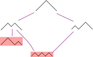
Figure 2. The ordinary Tamari lattice on $\mathcal{D}_{1,n}$ with $n=3$ (left), and its greedy counterpart (right). The shaded elements are minimal for the greedy order. The cover relations in the greedy order realize shortcuts in the ordinary Tamari lattice.

Figure 3. The ordinary Tamari lattice on $\mathcal{D}_{1,n}$ with $n=4$ (left), and its greedy counterpart (right). The chain above $11001100$ is order-isomorphic to the greedy order on $\mathcal{D}_{2,2}$.

Theorem 1.1.

The number of intervals in the greedy $m$-Tamari poset $\mathcal{D}_{m,n}$ is

$$\frac{(m+2)(m+1)^{n-1}}{(mn+1)(mn+2)}\binom{(m+1)n}{n}.$$

This is also the number of $(m+1)$-constellations having $n$ polygons.

Let us briefly recall from [7, 19] that an $m$-constellation is a rooted planar map (drawn on the sphere) whose faces are coloured black and white in such a way that

• all faces adjacent to a white face are black, and vice-versa,

• the degree of any black face is $m$,

• the degree of any white face is a multiple of $m$.

Constellations are rooted by distinguishing one of their edges. In Theorem 1.1, what we call polygon is a black face. We refer to [7] for an alternative description of constellations in terms of factorisations of permutations and for their bijective enumeration, to [8] for an alternative bijective approach, and to [14, Sec. 4.2] for a recursive approach.

Example 1.2.

When $m=n=2$, there are three $m$-Dyck paths of size $n$, namely

$$u=100100,\quad v=101000,\quad w=110000,$$

and the greedy $2$-Tamari order is the total order $u<v<w$. Hence there are $6$ greedy intervals, and we can check that the formula of Theorem 1.1 holds:

$$\frac{(2+2)(2+1)^{1}}{(2\cdot 2+1)(2\cdot 2+2)}\binom{(2+1)2}{2}=6.$$

The corresponding $6$ constellations with $n=2$ polygons (triangles, since $m+1=3$) are shown in Figure 4.

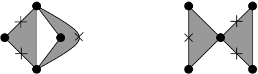
Figure 4. The six $3$-constellations with $2$ polygons. The crosses indicate the possible rootings.

Example 1.3.

Let us now take $m=1$ and $n=3$, and consider the greedy poset shown on the right of Figure 2: if we count, for all paths $u$ (taken from bottom to top and from left to right), the number of intervals of the form $[u,v]$, we find that the total number of intervals is

$$4+3+2+2+1=12=\frac{(1+2)(1+1)^{2}}{(3+1)(3+2)}\binom{2\cdot 3}{3}.$$

This is one less than the number of intervals in the ordinary Tamari lattice, shown on the left of Figure 2.

More generally, the number of intervals of $\mathcal{D}_{m,n}$ in the ordinary $m$-Tamari order is [5, 9]:

$$\frac{m+1}{n(mn+1)}{(m+1)^{2}n+m\choose n-1}.$$ (1)

These numbers first arose, conjecturally, in the study of polynomials in three sets of $n$ variables on which the symmetric group $\mathfrak{S}_{n}$ acts diagonally [1]. We are not aware of any occurrence of the numbers of Theorem 1.1 in such an algebraic context.

Our proof of Theorem 1.1 follows a recursive approach, similar to the proof of (1) in [5]. We begin in Section 2 with various definitions and constructions on Dyck paths and greedy Tamari intervals. In Section 3, we use them to write a functional equation for the generating function of these intervals (Proposition 3.1). This generating function records not only the size $n$ of the interval $[v,w]$ (defined as the common size of $v$ and $w$), but also the length of the longest suffix of down steps in $w$, called final descent of $w$. This parameter plays a “catalytic” role, in the sense that the functional equation cannot be written without it. Equations involving a catalytic variable abound in the enumeration of maps, and their solutions are systematically algebraic [6]. The enumeration of ordinary Tamari intervals also relies on a similar equation [5]. In Section 4, we solve our functional equation and express the bivariate generating function of intervals in terms of a pair of algebraic series (Theorem 4.1). In Section 5 we prove that our approach applies to ordinary $m$-Tamari intervals as well, and derive a new proof of (1), thus recovering the result of [5]. We conclude in Section 6 with a few comments and open questions. In particular, we conjecture the existence of a bijection between greedy intervals and constellations that would transform ascents of the top path into degrees of white faces (Conjecture 6.1).

As a side remark, our results were inspired by those obtained about the number of intervals in the so-called dexter semilattices in [10]. In fact, it is expected that the $m=1$ greedy Tamari posets are anti-isomorphic to the dexter posets, through a simple bijection that goes from Dyck paths to binary trees, performs a left-right-symmetry there and then comes back to Dyck paths by the same bijection.

2. $m$-Dyck paths and greedy partial order

Let us fix $m\geq 1$. We first complete the definitions introduced in the previous section.

The height of a vertex on an ($m$-)Dyck path is the $y$-coordinate of this vertex. A contact is a vertex of height $0$, distinct from the endpoints. A peak is an occurrence of a factor $10^{m}$. The unique Dyck path of size zero is called the empty Dyck path and denoted by $\varnothing$.

The final descent of a Dyck path $w$ is the longest suffix of the form $0^{k}$, and we denote its length by $d(w)=k$. If $w$ is non-empty, then $k\geq m$. Thus $w$ has at least one peak, consisting of the last up step and the $m$ down steps that follow it.

It is well known that every non-empty Dyck path $w$ admits a unique expression of the form $w=1(w_{1}0)(w_{2}0)\cdots(w_{m}0)w_{m+1}$, where $w_{1},\ldots,w_{m+1}$ are Dyck paths, possibly empty [20, Sec. 11.3]. We denote by $D(w_{1},\ldots,w_{m},w_{m+1})$ the Dyck path $1(w_{1}0)(w_{2}0)\cdots(w_{m}0)w_{m+1}$.

Let us now return to the greedy Tamari order defined in the introduction, and to its ordinary counterpart. For both orders, if $v\leq w$ then $v$ lies below $w$, in the sense that the height of the $i$th vertex of $v$ is at most the height of the $i$th vertex of $w$, for any $i$.

Moreover, the set $\mathcal{D}_{m,n}$ equipped with the greedy $m$-Tamari order is order-isomorphic to an upper ideal of $\mathcal{D}_{1,mn}$ equipped with the greedy $1$-Tamari order. The same statement was already true for the ordinary Tamari order [5, Prop. 4].

Proposition 2.1.

The greedy $m$-Tamari order on $\mathcal{D}_{m,n}$ is order-isomorphic to the greedy $1$-Tamari order on the upper ideal of $\mathcal{D}_{1,mn}$ consisting of paths in which the length of every ascent is a multiple of $m$ (by ascent, we mean a maximal sequence of up steps).

As in the ordinary case, the proof simply consists in replacing each up step of height $m$ in a path of $\mathcal{D}_{m,n}$ by a sequence of $m$ up steps of height $1$. The key property is that a cover relation may merge two ascents, but never splits an ascent into several parts. For instance, on the right of Figure 3, we recognize in the upper ideal generated by $11001100$ the greedy Tamari lattice on $\mathcal{D}_{2,2}$ described in Example 1.2.

2.1. A free monoid structure on $m$-Dyck paths

In the enumeration of ordinary $m$-Tamari intervals [5], a useful property is the fact that, for two Dyck paths $v$ and $w$ of the same length, with $w=w_{1}w_{2}$ written as the concatenation of two Dyck paths, we have $v\leq w$ if and only if $v=v_{1}v_{2}$ for two Dyck paths $v_{1}$ and $v_{2}$ such that $v_{1}\leq w_{1}$ and $v_{2}\leq w_{2}$. This leads to a recursive decomposition of ordinary intervals using the number of contacts (of the smaller element) as a catalytic variable. This property does not hold in the greedy case: for instance, when $m=1$ and $n=3$, the path $w=110010$ is not larger than $v=101010$, even though $w=w_{1}w_{2}$ and $v=v_{1}v_{2}$ with $v_{1}=1010<1100=w_{1}$ and $v_{2}=w_{2}=10$. This problem may not be irremediable, but in this paper we take another route. In fact, our approach also gives a new solution for ordinary $m$-Tamari intervals.

We define on $\mathcal{D}_{m}:=\cup_{n\geq 1}\mathcal{D}_{m,n}$ a new product, different from concatenation, and show that it endows $\mathcal{D}_{m}$ with a structure of graded free monoid. In the next subsection, we will see that this new product is, in a sense, compatible with the greedy order.

Let $w_{1}$ and $w_{2}$ be non-empty Dyck paths in $\mathcal{D}_{m}$. The product $w_{1}*w_{2}$ is defined as the Dyck path obtained by replacing the rightmost peak of $w_{1}$ by $w_{2}$ (Figure 5). One can check that this is associative, with unit the Dyck path $10^{m}$ made of a single peak. This product is moreover graded with degree the size minus $1$. Indeed, if we denote the size of $w$ by $|w|$, we have $|w_{1}*w_{2}|=|w_{1}|+|w_{2}|-1$, that is, $|w_{1}*w_{2}|-1=(|w_{1}|-1)+(|w_{2}|-1)$.

Figure 5. The monoid structure on $m$-Dyck paths, when $m=2$.

Here is an example with $m=2$, which shows that a path admits in general several expressions as a product:

$$1100{\color[rgb]{1,0,0}100}00*110000=1{\color[rgb]{1,0,0}100}00*100110000=110011000000.$$

This is because some of the factors can be further decomposed as products. In fact, we have the following unique factorisation property.

Proposition 2.2.

The set $\mathcal{D}_{m}$ equipped with the product $*$ is a free graded monoid on the generators $D(w_{1},w_{2},\dots,w_{i-1},10^{m},\varnothing,\dots,\varnothing)$, with $1\leq i\leq m+1$ and $w_{j}\in\mathcal{D}_{m}\cup\{\varnothing\}$ for all $j$.

Proof.

Let us first show that $\mathcal{D}_{m}$ is generated by these generators. Let $w$ be a non-empty Dyck path. Write $w=D(w_{1},w_{2},\dots,w_{m},w_{m+1})$. If all $w_{i}$’s are empty, then $w$ is the unit $10^{m}$. Otherwise, let $i$ be the largest index such that $w_{i}$ is non-empty, with $1\leq i\leq m+1$. Then $w=D(w_{1},\dots,w_{i-1},10^{m},\varnothing,\dots,\varnothing)*w_{i}$. This is the product of a generator by an element of $\mathcal{D}_{m}$, namely $w_{i}$, of smaller degree than $w$. Thus $\mathcal{D}_{m}$ is generated by the listed generators.

For instance, when $m=2$, the above path $w=110011000000$ can be iteratively factored as:

$$w =110000*100110000$$

$$=110000*100100*110000$$

$$=D(100,\varnothing,\varnothing)*D(\varnothing,\varnothing,100)*D(100,\varnothing,\varnothing).$$

We will now use comparison of generating functions to prove that the monoid is free. The generating function of $m$-Dyck paths, where the variable $t$ records the size, is the only formal power series $\mathbf{D}$ in the variable $t$ satisfying

$$\mathbf{D}=1+t\mathbf{D}^{m+1}.$$

This follows from the decomposition of Dyck paths as $D(w_{1},w_{2},\dots,w_{m},w_{m+1})$. The generators are counted by

$$\mathbf{G}:=t^{2}\sum_{i=1}^{m+1}\mathbf{D}^{i-1}=t^{2}\frac{\mathbf{D}^{m+1}-1}{\mathbf{D}-1}=t-\frac{t^{2}}{\mathbf{D}-1}.$$

Recall that the path $w_{1}*\cdots*w_{k}$ has size $|w_{1}|+\cdots+|w_{k}|-k+1$. Hence the free monoid on the listed generators has size generating function

$$\frac{t}{1-\mathbf{G}/t}=\mathbf{D}-1,$$

which coincides with the generating function of $\mathcal{D}_{m}$. This implies that there are no relations between the generators. ∎

Let us extract from the above proof an observation that will be useful later.

Lemma 2.3.

If $w=D(w_{1},\dots,w_{i-1},w_{i},\varnothing,\dots,\varnothing)$ with $w_{i}\not=\varnothing$, then the first factor in the factorisation of $w$ is $D(w_{1},\dots,w_{i-1},10^{m},\varnothing,\dots,\varnothing)$.

2.2. A free monoid structure on intervals

The monoid structure $*$ on $\mathcal{D}_{m}$ is compatible with the greedy Tamari order, in the following sense.

Proposition 2.4.

Let $v=v_{1}*v_{2}$ be a non-empty Dyck path. Let $v\triangleleft w$ be a greedy cover relation. Then either $w=w_{1}*v_{2}$ where $w_{1}$ covers $v_{1}$, or $w=v_{1}*w_{2}$ where $w_{2}$ covers $v_{2}$.

Conversely, every cover relation $v_{1}\triangleleft w_{1}$ gives a cover relation $v_{1}*v_{2}\triangleleft w_{1}*v_{2}$ and every cover relation $v_{2}\triangleleft w_{2}$ gives a cover relation $v_{1}*v_{2}\triangleleft v_{1}*w_{2}$.

Consequently, for any non-empty Dyck path $v=v_{1}*v_{2}$, the upper ideal $\{w:v\leq w\}$ is $\{w_{1}*w_{2}:v_{1}\leq w_{1}\text{ and }v_{2}\leq w_{2}\}$.

Proof.

Let us begin with the first statement. Consider the down step of the valley of $v$ involved in the cover relation $v\triangleleft w$. If this down step comes from $v_{1}$ (as in Figure 6), it is the first step of a valley of $v_{1}$, and hence defines a cover relation $v_{1}\triangleleft w_{1}$. This cover relation may or may not increase the height of the rightmost peak of $v_{1}$ (in the example of Figure 6 this height increases). In both cases, by definition of the product, one finds that $w_{1}*v_{2}=w$.

Figure 6. First type of cover relation $v\triangleleft w$ when $v=v_{1}*v_{2}$. The cover relation involves a down step of $v_{1}$.

If the down step involved in the cover relation $v\triangleleft w$ comes instead from $v_{2}$ (Figure 7), then the next up step also comes from $v_{2}$, hence it defines a cover relation $v_{2}\triangleleft w_{2}$. By definition of the product, one finds that $v_{1}*w_{2}=w$.

Figure 7. Second type of cover relation $v\triangleleft w$ when $v=v_{1}*v_{2}$. The cover relation involves a down step of $v_{2}$.

The second statement is checked similarly from the definitions, and the third one follows by iteration of cover relations. ∎

Figure 8. The monoid structure on greedy intervals, when $m=2$.

This lemma allows us to define a monoid structure on the set of all intervals of $\mathcal{D}_{m}=\cup_{n\geq 1}\mathcal{D}_{m,n}$ as follows. We intentionally use for this monoid the same symbol $*$ as for the monoid on Dyck paths.

Let $[v_{1},w_{1}]$ and $[v_{2},w_{2}]$ be intervals. By Proposition 2.4, we have $v_{1}*v_{2}\leq w_{1}*w_{2}$. We define the product $[v_{1},w_{1}]*[v_{2},w_{2}]$ to be the interval $[v_{1}*v_{2},w_{1}*w_{2}]$ (see Figure 8). For instance, for $m=1$ we have $[10{\color[rgb]{1,0,0}{10}},1{\color[rgb]{1,0,0}{10}}0]*[110010,111000]=[10110010,11110000]$. Since $*$ is associative on Dyck paths, it is also associative on intervals. The unit is the interval $[10^{m},10^{m}]$. We denote by $\mathcal{I}_{m}$ the monoid of intervals of positive size.

Proposition 2.5.

The monoid $\mathcal{I}_{m}$ is free over the generators $[v,w]$ where $v$ is a generator of the monoid $\mathcal{D}_{m}$, listed in Proposition 2.2, and $w$ any Dyck path larger than or equal to $v$.

Proof.

Let $[v,w]$ be an interval that is not the unit of $\mathcal{I}_{m}$. By unique factorisation in the monoid $\mathcal{D}_{m}$, one can write $v=v_{1}*v_{2}*\dots*v_{k}$ for some generators $v_{i}$. By Proposition 2.4, we have $w=w_{1}*w_{2}*\dots*w_{k}$ where $v_{i}\leq w_{i}$ for each $i$. Consequently, $[v,w]=[v_{1},w_{1}]*\cdots*[v_{k},w_{k}]$. Hence the elements $[v,w]$, for $v$ a generator of $\mathcal{D}_{m}$ and $w\geq v$, indeed generate the monoid $\mathcal{I}_{m}$.

For instance, for $m=1$ and the above interval $[v,w]=[10110010,11110000]$, the factorisation of $v$ is $v_{1}*v_{2}=1010*110010=D(\varnothing,10)*D(10,10)$. Hence we write $w$ as the product $w_{1}*w_{2}=1100*111000$ of a word of size $2$ and a word of size $3$, and obtain $[v,w]=[v_{1},w_{1}]*[v_{2},w_{2}]$.

Let us now pick any factorisation of $[v,w]$ as a product of generators $[v_{i},w_{i}]$. That is, $v=v_{1}*\cdots*v_{k}$ and $w=w_{1}*\cdots*w_{k}$ with $v_{i}\leq w_{i}$ for all $i$. Since the $v_{i}$’s are generators of the free monoid $\mathcal{D}_{m}$, the sequence $(v_{1},\ldots,v_{k})$ is uniquely determined by $v$. Moreover, given that $v_{i}$ and $w_{i}$ have the same size for every $i$, the sequence $(w_{1},\ldots,w_{k})$ is uniquely determined by $(v,w)$. (Indeed, given a product $u*u^{\prime}$, one can recover $u$ and $u^{\prime}$ from $u*u^{\prime}$ as soon as we know the size of $u^{\prime}$: one computes the unique factorization $u_{1}*\cdots*u_{\ell}$ of $u*u^{\prime}$ in the generators of Proposition 2.2, and then $u^{\prime}$ is the only factor $u_{j}*\cdots*u_{\ell}$, with $1\leq j\leq\ell$, that has the same size as $u^{\prime}$.) This proves uniqueness of the factorisation for the interval $[v,w]$, and concludes the proof. ∎

3. Recursive decomposition of greedy intervals

The aim of this section is to establish a functional equation that characterises the generating function $\mathbf{I}$ of greedy $m$-Tamari intervals. In the series $\mathbf{I}$, the interval $[v,w]$ is weighted by $t^{n}x^{d}$, where $n\geq 1$ is the common size of $v$ and $w$ (called the size of the interval) and $d=d(w)$ is the length of the final descent of $w$. The interval $[\varnothing,\varnothing]$ is thus not counted in $\mathbf{I}$. The functional equation for $\mathbf{I}$ involves the divided difference operator $\Delta$ defined by:

$$\Delta\mathbf{F}:=\frac{\mathbf{F}-\mathbf{F}(1)}{x-1},$$ (2)

where, for a formal power series $\mathbf{F}$ in $t$ with coefficients in $\mathbb{Q}[x]$ (the ring of polynomials in $x$), we denote by $\mathbf{F}(1)$ the specialisation of $\mathbf{F}$ at $x=1$.

Proposition 3.1.

The bivariate generating function $\mathbf{I}$ of greedy $m$-Tamari intervals is the unique solution of the following equation:

$$x^{2}\mathbf{I}=t(x+x^{2}\mathbf{I}\Delta)^{(m+2)}(1),$$

where the first $x$ in the operator $(x+x^{2}\mathbf{I}\Delta)$ stands for the multiplication by $x$, and the exponent $(m+2)$ means that the operator is applied $m+2$ times.

We will denote $\hat{\mathbf{I}}=x^{2}\mathbf{I}$, so that the above equation reads

$$\hat{\mathbf{I}}=t(x+\hat{\mathbf{I}}\Delta)^{(m+2)}(1).$$

Example. When $m=1$, the equation reads

$$\hat{\mathbf{I}} =t(x+\hat{\mathbf{I}}\Delta)^{(3)}(1)$$

$$=t(x+\hat{\mathbf{I}}\Delta)^{(2)}(x)$$

$$=t(x+\hat{\mathbf{I}}\Delta)(x^{2}+\hat{\mathbf{I}})$$

$$=tx(x^{2}+\hat{\mathbf{I}})+t\hat{\mathbf{I}}\left(x+1+\frac{\hat{\mathbf{I}}-\hat{\mathbf{I}}(1)}{x-1}\right).$$

In order to prove the above proposition, we first introduce several families of greedy intervals, and provide recursive decompositions for them. These decompositions translate into a system of functional equations for the corresponding bivariate generating functions. This system finally results in the above proposition. Solving the above functional equation (and in fact, the entire system) will be the topic of Section 4.

3.1. Some families of intervals

Recall that we only consider intervals of positive size, ignoring the interval $[\varnothing,\varnothing]$. The set of all such intervals has been so far denoted by $\mathcal{I}_{m}$ so far, but we will now drop the index $m$ and simply write $\mathcal{I}$. We introduce the following collection of subsets of $\mathcal{I}$.

Definition 3.2.

For $i\in\llbracket 0,m+1\rrbracket$, let $\mathcal{J}_{i}$ denote the set of intervals $[v,w]$ such that the minimum $v$ is of the form $D(v_{1},v_{2},\dots,v_{i},\varnothing,\varnothing,\dots,\varnothing)$, for some $v_{1},\ldots,v_{i}$ in $\mathcal{D}_{m}\cup\{\varnothing\}$.

Observe that $\mathcal{J}_{0}$ only contains the unit interval $[10^{m},10^{m}]$, and that $\mathcal{J}_{m+1}=\mathcal{I}$. Denoting by $\mathbf{J}_{i}$ the bivariate generating function of $\mathcal{J}_{i}$, we will establish the following system:

$$\left\{\begin{array}[]{ll}\mathbf{J}_{0}&=x^{m}t,\\ \mathbf{J}_{i}&=\displaystyle\mathbf{J}_{i-1}+\mathbf{I}\frac{x\mathbf{J}_{i-1}-x^{m+1-i}\mathbf{J}_{i-1}(1)}{x-1}\qquad\text{for }i>0.\\ \end{array}\right.$$

As explained in Section 3.4, Proposition 3.1 easily follows.

As an intermediate step in the decomposition of the intervals of $\mathcal{J}_{i}$, it will be convenient to introduce the following subset of $\mathcal{J}_{i}$.

Definition 3.3.

For $i\in\llbracket 1,m+1\rrbracket$, let $\mathcal{K}_{i}$ denote the subset of $\mathcal{J}_{i}$ consisting of intervals $[v,w]$ such that $v$ is of the form $D(v_{1},v_{2},\dots,v_{i-1},10^{m},\varnothing,\varnothing,\dots,\varnothing)$.

The associated bivariate generating function is denoted by $\mathbf{K}_{i}$.

3.2. Description of $\mathcal{J}_{i}$

If $i=0$, then $\mathcal{J}_{i}=\mathcal{J}_{0}$ is reduced to $[10^{m},10^{m}]$, so that $×\mathbf{J}_{0}=x^{m}t$. We now assume $i\geq 1$.

Let $[v,w]$ be an interval of $\mathcal{J}_{i}$, and write $v=D(v_{1},\ldots,v_{i},\varnothing,\ldots,\varnothing)$. If $v_{i}=\varnothing$, then $[v,w]$ is any interval of $\mathcal{J}_{i-1}$. Let us now assume that $v_{i}\not=\varnothing$. Let us write $[v,w]=[v^{\prime},w^{\prime}]*[v^{\prime\prime},w^{\prime\prime}]$, where $[v^{\prime},w^{\prime}]$ is a generator of the free monoid $\mathcal{I}_{m}\equiv\mathcal{I}$ (see Proposition 2.5). Recall that $v^{\prime}$ is also the first factor in the factorisation of $v$ in the free monoid $\mathcal{D}_{m}$, so that, by Lemma 2.3, $v^{\prime}=D(v_{1},\dots,v_{i-1},10^{m},\varnothing,\ldots,\varnothing)$ (and $v^{\prime\prime}=v_{i}$). This means that $[v^{\prime},w^{\prime}]$ belongs to $\mathcal{K}_{i}$. Let us denote $\phi([v,w])=([v^{\prime},w^{\prime}],[v^{\prime\prime},w^{\prime\prime}])$ (see Figure 9).

For instance, for $m=1$ and $[v,w]=[110100101100,110111100000]$, we have $v=D(1010,\allowbreak 101100)$ so that $[v,w]\in\mathcal{J}_{2}$. The path $v$ factors as $v=v^{\prime}*v^{\prime\prime}$ with $v^{\prime}=11010010=D(1010,10)$ and $v^{\prime\prime}=101100$. The interval $[v,w]$ decomposes as $[v^{\prime},w^{\prime}]*[v^{\prime\prime},w^{\prime\prime}]$ where $w^{\prime}=11011000$ and $w^{\prime\prime}=111000$, and indeed $[v^{\prime},w^{\prime}]\in\mathcal{K}_{2}$.

Conversely, take $[v^{\prime},w^{\prime}]$ in $\mathcal{K}_{i}$, and $[v^{\prime\prime},w^{\prime\prime}]$ in $\mathcal{I}$. Observe that $v^{\prime}$ is a generator of $\mathcal{D}_{m}$, and $[v^{\prime},w^{\prime}]$ a generator of $\mathcal{I}_{m}$. Form the interval $[v,w]:=[v^{\prime},w^{\prime}]*[v^{\prime\prime},w^{\prime\prime}]$. Then $[v^{\prime},w^{\prime}]$ is the first generator in the factorisation of $[v,w]$ and $\phi([v,w])=([v^{\prime},w^{\prime}],[v^{\prime\prime},w^{\prime\prime}])$.

We have thus described a bijection $\phi$ that maps $\mathcal{J}_{i}\setminus\mathcal{J}_{i-1}$ onto $\mathcal{K}_{i}\times\mathcal{I}$. Moreover, if $\phi([v,w])=([v^{\prime},w^{\prime}],[v^{\prime\prime},w^{\prime\prime}])$, then $|w|=|w^{\prime}|+|w^{\prime\prime}|-1$ and the final descent of $w$ has length $d(w)=d(w^{\prime})+d(w^{\prime\prime})-m$. This gives the following identity:

$${\mathbf{J}_{i}}=\mathbf{J}_{i-1}+\frac{\mathbf{K}_{i}}{x^{m}t}{\mathbf{I}}.$$ (3)

Figure 9. Decomposition of an interval $[v,w]$ of $\mathcal{J}_{i}\setminus\mathcal{J}_{i-1}$, with $m=2$ and $i=2$.

3.3. Description of $\mathcal{K}_{i}$

Let us begin with a simple observation.

Lemma 3.4.

Consider a cover relation $v\triangleleft w$, where $v$ and $w$ are non-empty. Let $v^{\prime}$ (resp. $w^{\prime}$) be obtained by deleting the last peak of $v$ (resp. $w$). Then either $v^{\prime}=w^{\prime}$ (if the cover relation takes place in the last valley of $v$) or otherwise $v^{\prime}\triangleleft w^{\prime}$. Consequently, if $v\leq w$ and $v^{\prime}$ and $w^{\prime}$ are obtained as above, then $v^{\prime}\leq w^{\prime}$.

Now let $i\in\llbracket 1,m+1\rrbracket$, and consider an interval $[v,w]$ in $\mathcal{K}_{i}$. By definition, this means that $v=D(v_{1},\ldots,v_{i-1},10^{m},\varnothing,\ldots,\varnothing)$. Let us define $v^{\prime}$ and $w^{\prime}$ by deleting the last peak of $v$ and $w$, respectively. By Lemma 3.4, we obtain an interval $[v^{\prime},w^{\prime}]$. Moreover, $v^{\prime}=D(v_{1},\ldots,v_{i-1},\varnothing,\ldots,\varnothing)$, so that $[v^{\prime},w^{\prime}]$ is in $\mathcal{J}_{i-1}$. To recover $v$ from $v^{\prime}$, it suffices to insert the factor $10^{m}$ in the final descent of $v^{\prime}$, at height $m+1-i$ (by this, we mean that the final up step of $v$ starts at height $m+1-i$). Analogously, we recover $w$ from $w^{\prime}$ by inserting a peak in the final descent of $w^{\prime}$. Note that its insertion height $h$ is at least $m+1-i$ (so that $w$ is above $v$) and at most $d(w^{\prime})$. Let us denote $\psi([v,w]):=([v^{\prime},w^{\prime}],h)$.

For instance, take $m=1$ and $[v,w]=[11010010,11011000]$. We have $v=D(1010,10)$ so that $[v,w]\in\mathcal{K}_{2}$. Removing the final peaks of $v$ and $w$ gives $v^{\prime}=110100=w^{\prime}$. In particular, $[v^{\prime},w^{\prime}]$ is trivially an interval. We recover $v$ from $v^{\prime}$ by inserting a peak $10$ in $v^{\prime}$ at height $0$, and we recover $w$ from $w^{\prime}$ by inserting $10$ at height $2$. Hence $\psi([v,w]):=([110100,110100],2)$.

The converse construction is illustrated in Figure 10. Take $[v^{\prime},w^{\prime}]$ in $\mathcal{J}_{i-1}$, and write $v^{\prime}=D(v_{1},\ldots,v_{i-1},\varnothing,\ldots,\varnothing)$. Form the path $v:=D(v_{1},\ldots,v_{i-1},10^{m},\varnothing,\ldots,\varnothing)$. Choose $h\in\llbracket m+1-i,d(w^{\prime})\rrbracket$, and let $w$ be obtained by inserting $10^{m}$ in the final descent of $w^{\prime}$, at height $h$. Let us also introduce an intermediate path $w_{0}$, obtained by inserting a peak at height $m+1-i$ in the final descent of $w^{\prime}$. Let us now prove that $v\leq w_{0}\leq w$. Let us choose a sequence of cover relations from $v^{\prime}$ to $w^{\prime}$. Since they take place at valleys of height $>m+1-i$ (there is no lower valley in $v^{\prime}$), performing cover relations at the same places in $v$ gives a sequence of cover relations from $v$ to $w_{0}$; see Figure 10(2). Now starting from $w_{0}$, we perform a sequence of cover relations taking place systematically in the last valley, until the final peak starts at height $h\leq d(w^{\prime})$. These cover relations only move the last peak up; see Figure 10(3). Thus $v\leq w$, and the interval $[v,w]$ belongs to $\mathcal{K}_{i}$ since $v=D(v_{1},\ldots,v_{i-1},10^{m},\varnothing,\ldots,\varnothing)$. Moreover, $\psi([v,w])=([v^{\prime},w^{\prime}],h)$.

Figure 10. From an interval $[v^{\prime},w^{\prime}]$ in $\mathcal{J}_{i-1}$ and a height $h$ in $\llbracket m+1-i,d(w^{\prime})\rrbracket$ to an interval $[v,w]$ in $\mathcal{K}_{i}$. Here, $m=2$, $i=2$ and $h=7$.

We have thus described a bijection $\psi$ between $\mathcal{K}_{i}$ and the set of pairs $([v^{\prime},w^{\prime}],h)$ such that $[v^{\prime},w^{\prime}]\in\mathcal{J}_{i-1}$ and $h\in\llbracket m+1-i,d(w^{\prime})\rrbracket$. Moreover, if $\psi([v,w])=([v^{\prime},w^{\prime}],h)$, then $|v|=1+|v^{\prime}|$ and $d(w)=m+h$. In terms of generating functions, this gives

$$\mathbf{K}_{i}=\sum_{[v^{\prime},w^{\prime}]\in\mathcal{J}_{i-1}}t^{1+|v^{\prime}|}\sum_{h=m+1-i}^{d(w^{\prime})}x^{m+h}=x^{m}t\frac{x\mathbf{J}_{i-1}-x^{m+1-i}\mathbf{J}_{i-1}(1)}{x-1}.$$ (4)

3.4. Proof of Proposition 3.1

We now combine the above functional equations into a single equation defining $\mathbf{I}$. First, we use (4) to rewrite the expression (3) of $\mathbf{J}_{i}$. For $1\leq i\leq m+1$, we thus obtain

$$\mathbf{J}_{i}=\mathbf{J}_{i-1}+\mathbf{I}\frac{x\mathbf{J}_{i-1}-x^{m+1-i}\mathbf{J}_{i-1}(1)}{x-1},$$

or equivalently,

$$\frac{\mathbf{J}_{i}}{x^{m-i-1}}=\left(x+x^{2}\mathbf{I}\Delta\right)\left(\frac{\mathbf{J}_{i-1}}{x^{m-i}}\right),$$ (5)

where $\Delta$ is the divided difference operator (2). Using $\mathbf{J}_{0}=x^{m}t$, this can be solved by induction on $i$ as

$$\frac{\mathbf{J}_{i}}{x^{m-i-1}}=\left(x+x^{2}\mathbf{I}\Delta\right)^{(i)}(xt)=t\left(x+x^{2}\mathbf{I}\Delta\right)^{(i+1)}(1).$$

Given that $\mathbf{I}=\mathbf{J}_{m+1}$, this gives the equation of Proposition 3.1. ∎

4. Solution of the functional equation

In this section, we solve the functional equation defining the series $\mathbf{I}$ in Proposition 3.1. For any $m$, this is an equation in one “catalytic” variable $x$, in the terminology of [6]. In particular, it follows from the latter reference that $\mathbf{I}$ is an algebraic series. That is, it satisfies a non-trivial polynomial equation with coefficients in $\mathbb{Q}[x,t]$. Moreover, one can also use the tools developed in [6], and very recently in [3], to construct an explicit algebraic equation satisfied by $\mathbf{I}$, for small values of $m$. However, the difficulty here is to determine $\mathbf{I}$ for an arbitrary value of $m$.

The functional equation satisfied by $\mathbf{I}$ is reminiscent of the equation satisfied by a bivariate generating function $\mathbf{T}$ of ordinary Tamari intervals in $\mathcal{D}_{m,n}$, $n\geq 0$, which was established in [5, Prop. 8], and reads:

$$\mathbf{T}=x+xt\left(\mathbf{T}\Delta\right)^{(m+1)}(x).$$ (6)

It is also reminiscent of an equation derived in [14, Thm. 4.1] for planar $(m+1)$-constellations, which reads:

$$\mathbf{C}=1+xt(\mathbf{C}+\Delta)^{(m+1)}(1).$$ (7)

In the latter equation, $t$ records the number of polygons and $x$ the degree of the white root face, divided by $(m+1)$. For $m=2$, the solution to this equation starts

$$\mathbf{C}=1+tx+t^{2}\left(3x^{2}+3x\right)+\mathcal{O}(t^{3}),$$

(see Figure 4) while the series counting greedy $m$-Tamari intervals reads

$$\mathbf{I}=tx^{2}+t^{2}\left(3x^{2}+2x+1\right)+\mathcal{O}(t^{3}).$$

Hence, even though we will prove that $1+\mathbf{I}(1)=\mathbf{C}(1)$ (for any $m$), the catalytic parameters do not match. We believe that the catalytic parameter used for constellations corresponds to the length of the first ascent of the maximal element in greedy intervals, and refer to Section 6.1 for a much refined conjecture.

Our approach to solve the equation of Proposition 3.1 is similar to the one used in [5]: by examination of the solution for small values of $m$, we guess a general parametric form of the solution, valid for any $m$, and then check that this guess satisfies the functional equation. More precisely, we guess the value of all series $\mathbf{J}_{i}$, for $1\leq i\leq m+1$, and prove that these values satisfy the system (5).

We introduce a rational parametrization of $t$ and $x$ by two formal power series in $t$ denoted $\mathbf{Z}$ and $\mathbf{U}$. The series $\mathbf{Z}$ has integer coefficients, while $\mathbf{U}$ has coefficients in $\mathbb{Q}[x]$. The series $\mathbf{Z}$ is the unique formal power series in $t$ with constant term $0$ such that

$$t=\mathbf{Z}{(1-m^{+}\mathbf{Z})^{m}},$$

where we denote $m^{+}:=m+1$ to avoid having too many parentheses around, and $\mathbf{U}$ is the unique formal power series in $t$ such that

$$x=\frac{\mathbf{U}}{1-m^{+}\mathbf{Z}}\left(1-\mathbf{Z}\frac{\mathbf{U}^{m+1}-1}{\mathbf{U}-1}\right).$$ (8)

We have

$$\mathbf{Z}=t+\mathcal{O}(t^{2})\qquad\text{and}\qquad\mathbf{U}=x+xt\left(\frac{x^{m+1}-1}{x-1}-m^{+}\right)+\mathcal{O}(t^{2}).$$

Note also that $\mathbf{U}(1)=1$. We have found a rational expression of $\mathbf{I}$, and in fact of all series $\mathbf{J}_{i}$ with $0\leq i\leq{m+1}$, in terms of the series $\mathbf{Z}$ and $\mathbf{U}$.

Theorem 4.1.

The bivariate generating function  $\mathbf{I}$ of intervals in the greedy $m$-Tamari posets, counted by the size and the final descent of the maximal element, is given by:

$$x^{2}\mathbf{I}=\frac{\mathbf{Z}\mathbf{U}^{m+2}}{(1-m^{+}\mathbf{Z})^{2}}\left(1-\mathbf{Z}\sum_{e=0}^{m}\mathbf{U}^{e}(m+1-e)\right)=\frac{\mathbf{Z}\mathbf{U}^{m+2}}{1-m^{+}\mathbf{Z}}\cdot\frac{x-1}{\mathbf{U}-1}.$$ (9)

In particular, the size generating function of greedy $m$-Tamari intervals is

$$\mathbf{I}(1)=\frac{\mathbf{Z}}{(1-m^{+}\mathbf{Z})^{2}}\left(1-\binom{m+2}{2}\,\mathbf{Z}\right).$$

More generally, for $0\leq i\leq m+1$, the bivariate series $\mathbf{J}_{i}$ that counts the intervals of the set $\mathcal{J}_{i}$ (see Definition 3.2) is given by:

$$\frac{\mathbf{J}_{i}}{x^{m-i-1}}=\mathbf{Z}(1-m^{+}\mathbf{Z})^{m-i-1}\mathbf{\mathbf{H}}_{i}(\mathbf{Z};\mathbf{U}),$$ (10)

where $\mathbf{H}_{i}(z;u)\equiv\mathbf{H}_{i}(u)$ is a polynomial in $z$ and $u$ given by:

$$\mathbf{H}_{m+1}(u)=u^{m+2}\left(1-z\sum_{e=0}^{m}u^{e}(m+1-e)\right),$$ (11)

and for $0\leq i\leq m$,

$$\mathbf{H}_{i}(u)=u^{i+1}\left(1+\sum_{k=1}^{i+1}(-z)^{k}\binom{i+1}{k}\sum_{e=0}^{m-i}\binom{e+k-1}{e}u^{e}+\sum_{k=1}^{i}(-z)^{k}\binom{m+k-i-1}{k-1}\sum_{e=0}^{i-k}\binom{e+k}{e}u^{m+1-k-e}\right).$$ (12)

Remark. We can apply the Lagrange inversion formula to the series $\mathbf{Z}$ and the above expression of $\mathbf{I}(1)$, and this gives the expression of Theorem 1.1 for the number of greedy Tamari intervals in $\mathcal{D}_{m,n}$. The coefficients of the bivariate series $\mathbf{I}$ do not seem to factor nicely.

Proof.

Let us denote $\hat{\mathbf{J}}_{i}:=\mathbf{J}_{i}/x^{m-i-1}$ for $i=0,\dots,m+1$. Recall that we have also denoted $\hat{\mathbf{I}}=x^{2}\mathbf{I}=\hat{\mathbf{J}}_{m+1}$. The functional equations (5) become, for $1\leq i\leq m+1$,

$$\hat{\mathbf{J}}_{i}=\left(x+\hat{\mathbf{I}}\Delta\right)\hat{\mathbf{J}}_{i-1}.$$ (13)

Together with the initial condition $\hat{\mathbf{J}}_{0}=xt$, and the fact that the series $\hat{\mathbf{J}}_{i}$ have no constant term in $t$ (as they count intervals of positive size), these equations define each $\hat{\mathbf{J}}_{i}$ uniquely as a formal power series in $t$. Indeed, the coefficient of $t^{n}$ in $\hat{\mathbf{J}}_{i}$ is a polynomial in $x$ that can be computed by a double induction on $n$ and $i$. It is clear on (9) and (10) that the claimed values of $\hat{\mathbf{I}}$ and $\hat{\mathbf{J}}_{i}$ have no constant term in $t$, and moreover one readily checks that the right-hand side of (10) reduces to $xt$ when $i=0$, as expected. Thus it suffices to prove that the series $\hat{\mathbf{I}}$ and $\hat{\mathbf{J}}_{i}$ of Theorem 4.1 satisfy all the equations (13). We will see that these equations simplify nicely once rewritten in terms of $\mathbf{Z}$ and $\mathbf{U}$.

Let $\mathbf{H}(u)$ be an arbitrary polynomial in $u$, and recall that the series $\mathbf{U}$ defined by (8) equals $1$ when $x=1$. Hence, if $\hat{\mathbf{I}}$ is given by the right-hand side of (9), we have

$$\left(x+\hat{\mathbf{I}}\Delta\right)\left(\mathbf{H}(\mathbf{U})\right)=\frac{\mathbf{U}}{1-m^{+}\mathbf{Z}}\left(\mathbf{H}(\mathbf{U})+\mathbf{Z}\,\frac{\mathbf{H}(\mathbf{U})-\mathbf{U}^{m+1}\mathbf{H}(1)}{\mathbf{U}-1}\right).$$

Hence the series $\hat{\mathbf{J}}_{i}=\mathbf{J}_{i}/x^{m-i-1}$ given by (10) satisfy the system (13) if and only if, for $1\leq i\leq m+1$,

$$\mathbf{H}_{i}(\mathbf{U})=\mathbf{U}\left(\mathbf{H}_{i-1}(\mathbf{U})+\mathbf{Z}\,\frac{\mathbf{H}_{i-1}(\mathbf{U})-\mathbf{U}^{m+1}\mathbf{H}_{i-1}(1)}{\mathbf{U}-1}\right).$$

This system holds with the series $\mathbf{H}_{i}(z;u)$ evaluated at $(\mathbf{Z},\mathbf{U})$ if it holds with indeterminates $(z,u)$, that is, if for $1\leq i\leq m+1$,

$$\mathbf{H}_{i}(u)=u\mathbf{H}_{i-1}(u)+zu\,\frac{\mathbf{H}_{i-1}(u)-u^{m+1}\mathbf{H}_{i-1}(1)}{u-1}.$$ (14)

In short,

$$\mathbf{H}_{i}=\left(u+z\nabla_{m}\right)\left(\mathbf{H}_{i-1}(u)\right),$$

where the operator $\nabla_{m}$ is defined by

$$\nabla_{m}\mathbf{H}=u\frac{\mathbf{H}-u^{m+1}\mathbf{H}(1)}{u-1}.$$ (15)

This is now a polynomial identity, which we prove in Appendix A using basic binomial identities. ∎

5. A new solution for ordinary $m$-Tamari intervals

In this section, we show how to adapt the decomposition of greedy $m$-Tamari intervals used in Section 3 to count ordinary $m$-Tamari intervals. We thus obtain a second proof of the result of [5], giving the number of such intervals in $\mathcal{D}_{m,n}$ in the form (1). Moreover, we refine this result by recording the length of the final descent in the upper path of the interval (Theorem 5.4), while the result of [5] was recording instead the number of contacts of the lower path (and the length of the first ascent of the upper path).

The key difference with what has been done in Section 3 for greedy intervals is that we now only consider factorisations of $m$-Dyck paths $v$ of the form $v_{1}*v_{2}$ such that $v_{2}$ is prime, that is, has no contact (recall that the endpoints do not count as contacts). The proofs are very close to the greedy case, and we will be a bit more sketchy in this section. We will use the following counterpart of Proposition 2.2 and Lemma 2.3.

Lemma 5.1.

Let $v=D(v_{1},\ldots,v_{j-1},v_{j},\varnothing,\ldots,\varnothing)\in\mathcal{D}_{m,n}$, with $v_{j}\not=\varnothing$. Then $v$ can be written in a unique way as $v^{\prime}*v^{\prime\prime}$, where $v^{\prime}$ is of the form $D(v^{\prime}_{1},\ldots,v^{\prime}_{j-1},v^{\prime}_{j}10^{m},\varnothing,\ldots,\varnothing)$ and $v^{\prime\prime}$ is prime.

Proof.

Write $v_{j}=v^{\prime}_{j}10^{m}*v^{\prime\prime}$, where $v^{\prime\prime}$ is prime. Clearly, there is a unique way of doing this (the path $v^{\prime\prime}$ is the unique prime Dyck path that is a suffix of $v_{j}$). Then the only factorisation of $v$ that satisfies the conditions of the lemma is obtained with $v^{\prime}_{i}=v_{i}$ for $1\leq i<j$. ∎

For instance, when $m=2$, the path $v=110011000000=D(100110000,\varnothing,\varnothing)$ factors as $D(100100,\varnothing,\varnothing)*110000$, and $v^{\prime\prime}:=110000$ is prime.

We now have the following counterpart of Proposition 2.4.

Proposition 5.2.

Let $v=v_{1}*v_{2}$ be a non-empty Dyck path, and assume that $v_{2}$ is prime. Let $v\triangleleft w$ be an ordinary Tamari cover relation. Then either $w=w_{1}*v_{2}$ where $w_{1}$ covers $v_{1}$, or $w=v_{1}*w_{2}$ where $w_{2}$ covers $v_{2}$.

Conversely, every cover relation $v_{1}\triangleleft w_{1}$ gives a cover relation $v_{1}*v_{2}\triangleleft w_{1}*v_{2}$ and every cover relation $v_{2}\triangleleft w_{2}$ gives a cover relation $v_{1}*v_{2}\triangleleft v_{1}*w_{2}$.

Consequently, for any non-empty Dyck path $v=v_{1}*v_{2}$, with $v_{2}$ prime, the upper ideal $\{w:v\leq w\}$ is $\{w_{1}*w_{2}:v_{1}\leq w_{1}\text{ and }v_{2}\leq w_{2}\}$.

This proposition allows us to define the product $[v_{1},w_{1}]*[v_{2},w_{2}]$, again as $[v_{1}*v_{2},w_{1}*w_{2}]$, but now under the assumption that $v_{2}$ is prime. Note that this implies that $w_{2}$ is prime too.

5.1. Recursive description of ordinary intervals

As before, we only consider (ordinary) intervals of positive size. Let us denote by $\overline{\mathcal{I}}\equiv\overline{\mathcal{I}}_{m}$ the set of such intervals. For $1\leq i\leq m+1$, let $\overline{\mathcal{J}}_{i}$ be the set of intervals $[v,w]$ such that $v=D(v_{1},\ldots,v_{i-1},v_{i},\varnothing,\ldots,\varnothing)$. Finally, let $\overline{\mathcal{K}}_{i}$ be the subset of $\overline{\mathcal{J}}_{i}$ consisting of intervals $[v,w]$ such that $v=D(v_{1},\ldots,v_{i-1},v_{i}10^{m},\varnothing,\ldots,\varnothing)$. The associated generating functions are denoted by $\mathbf{\overline{I}}$, $\mathbf{\overline{J}}_{i}$ and $\mathbf{\overline{K}}_{i}$, respectively. Observe that $\overline{\mathcal{J}}_{0}$ only contains the unit interval $[10^{m},10^{m}]$, while $\overline{\mathcal{J}}_{m+1}$ coincides with $\overline{\mathcal{I}}$.

Proposition 5.3.

The series $\mathbf{\overline{J}}_{i}$, for $0\leq i\leq m+1$, are given by $\mathbf{\overline{J}}_{0}=x^{m}t$ and the equations:

$$\mathbf{\overline{J}}_{i}=\mathbf{\overline{J}}_{i-1}+\mathbf{\overline{J}}_{m}\frac{x\mathbf{\overline{J}}_{i}-x^{m+1-i}\mathbf{\overline{J}}_{i}(1)}{x-1},\qquad\text{for }1\leq i\leq m+1.$$

Recall that $\mathbf{\overline{J}}_{m+1}$ coincides with the bivariate generating function $\mathbf{\overline{I}}$ of ordinary $m$-Tamari intervals.

Proof.

The proof follows the same steps as in Section 3. First, if $[v,w]\in\overline{\mathcal{J}}_{i}\setminus\overline{\mathcal{J}}_{i-1}$, we write $v=v^{\prime}*v^{\prime\prime}$ as in Lemma 5.1. By Proposition 5.2, we have $[v,w]=[v^{\prime},w^{\prime}]*[v^{\prime\prime},w^{\prime\prime}]$. The map that sends $[v,w]$ to the pair $([v^{\prime},w^{\prime}],[v^{\prime\prime},w^{\prime\prime}])\in\overline{\mathcal{K}}_{i}\times\overline{\mathcal{J}}_{m}$ is easily seen to be bijective. This is the counterpart of Section 3.2, and gives

$$\mathbf{\overline{J}}_{i}=\mathbf{\overline{J}}_{i-1}+\frac{\mathbf{\overline{K}}_{i}}{x^{m}t}\mathbf{\overline{J}}_{m}.$$

For instance, take $m=1$ and consider the interval $[v,w]=[110100101100,110111100000]$, already considered in the greedy case (Section 3.2). The factorisation that we use is now $[v^{\prime},w^{\prime}]*[v^{\prime\prime},w^{\prime\prime}]$ where $v^{\prime}=D(1010,1010)$, $v^{\prime\prime}=1100$, $w^{\prime}=1101110000$ and $w^{\prime\prime}=1100=v^{\prime\prime}$.

Let us now decompose intervals of $\overline{\mathcal{K}}_{i}$. First, we check that Lemma 3.4 holds verbatim for ordinary $m$-Tamari intervals. Now take $[v,w]\in\overline{\mathcal{K}}_{i}$, with $v=D(v_{1},\ldots,v_{i}10^{m},\varnothing,\ldots,\varnothing)$. Define $v^{\prime}$ (resp. $w^{\prime}$) by deleting the last peak of $v$ (resp. $w$). In particular, $v^{\prime}=D(v_{1},\ldots,v_{i},\varnothing,\ldots,\varnothing)$, so that the interval $[v^{\prime},w^{\prime}]$ belongs to $\overline{\mathcal{J}}_{i}$. Let $h$ be the height of the starting point of the last up step in $w$. Again, we have the natural bounds $h\in\llbracket m+1-i,d(w^{\prime})\rrbracket$. The map $\psi$ defined by $\psi([v,w])=([v^{\prime},w^{\prime}],h)$ is easily seen to be a bijection from $\overline{\mathcal{K}}_{i}$ to $\{([v^{\prime},w^{\prime}],h)\in\overline{\mathcal{J}}_{i}\times\mathbb{N}:m+1-i\leq h\leq d(w")\}$, and the equation

$$\mathbf{\overline{K}}_{i}=x^{m}t\frac{x\mathbf{\overline{J}}_{i}-x^{m+1-i}\mathbf{\overline{J}}_{i}(1)}{x-1}$$

is obtained as the counterpart of (4). We now combine this equation with the previous one to complete the proof of the proposition. ∎

Remark. When $m=1$, it is known that the length of the last descent of the upper path $w$ in ordinary intervals $[v,w]$ is distributed as the number of contacts in the lower path $v$, plus one (in fact, the joint distribution is symmetric, see [5, Sec. 4]). In terms of generating functions, this means that $\mathbf{\overline{I}}=\mathbf{T}/x-1$, where $\mathbf{T}$ is the solution of (6) when $m=1$. We could thus expect that the functional equation obtained for $\mathbf{\overline{I}}=\mathbf{\overline{J}}_{2}$ by elimination of $\mathbf{\overline{J}}_{1}$ in the system of Proposition 5.3 coincides with the one derived from (6). This is however not the case: the former equation involves the series $\mathbf{\overline{J}}(1)$ and $\mathbf{\overline{J}}^{\prime}(1)$, while the latter only involves $\mathbf{\overline{J}}(1)$. Mixing both equations provides a relation between these two series.

5.2. Solution

As before, we introduce a rational parametrization of $t$ and $x$ by two formal power series in $t$ denoted $\mathbf{\overline{Z}}$ and $\mathbf{\overline{U}}$. The series $\mathbf{\overline{Z}}$ has integer coefficients, while $\mathbf{\overline{U}}$ has coefficients in $\mathbb{Q}[x]$. The series $\mathbf{\overline{Z}}$ is the unique formal power series in $t$ with constant term $0$ such that

$$t=\mathbf{\overline{Z}}\left(1-\mathbf{\overline{Z}}\right)^{m^{2}+2m},$$

and $\mathbf{\overline{U}}$ is the unique formal power series in $t$ such that

$$x=\frac{\mathbf{\overline{U}}}{(1-\mathbf{\overline{Z}})^{m+2}}\left(1-\mathbf{\overline{Z}}\frac{\mathbf{\overline{U}}^{m+1}-1}{\mathbf{\overline{U}}-1}\right).$$

We have

$$\mathbf{\overline{Z}}=t+\mathcal{O}(t^{2})\qquad\text{and}\qquad\mathbf{\overline{U}}=x+xt\left(\frac{x^{m+1}-1}{x-1}-(m+2)\right)+\mathcal{O}(t^{2}).$$

Note that $\mathbf{\overline{U}}(1)=1-\mathbf{\overline{Z}}$.

Theorem 5.4.

The bivariate generating function  $\mathbf{\overline{I}}$ of intervals in the ordinary $m$-Tamari lattices, counted by the size and the final descent of the maximal element, is given by:

$$x^{2}\mathbf{\overline{I}}=\frac{\mathbf{\overline{Z}}\,\mathbf{\overline{U}}^{m+2}}{(1-\mathbf{\overline{Z}})^{2m+4}}\left(1-\mathbf{\overline{Z}}\sum_{e=0}^{m}\mathbf{\overline{U}}^{e}(m+1-e)\right).$$

In particular, the size generating function of ordinary $m$-Tamari intervals satisfies

$$1+\mathbf{\overline{I}}(1)=\frac{1-(m+1)\mathbf{\overline{Z}}}{(1-\mathbf{\overline{Z}})^{m+2}},$$

as already established in [5]. We then recover (1) using the Lagrange inversion formula.

Moreover, we have

$$\mathbf{\overline{J}}_{m}=\frac{x-1}{x}\cdot\frac{\mathbf{\overline{Z}}\,\mathbf{\overline{U}}^{m+1}}{\mathbf{\overline{U}}-1+\mathbf{\overline{Z}}},$$ (16)

More generally, for $0\leq i\leq m+1$, the bivariate series $\mathbf{\overline{J}}_{i}$ is given by:

$$\frac{\mathbf{\overline{J}}_{i}}{x^{m-i-1}}=\mathbf{\overline{Z}}\left(1-\mathbf{\overline{Z}}\right)^{(m+2)(m-i-1)}\mathbf{H}_{i}\left(\mathbf{\overline{Z}};\mathbf{\overline{U}}\right),$$ (17)

where the polynomials $\mathbf{H}_{i}(z;u)\equiv\mathbf{H}_{i}(u)$ are defined in (11)-(12).

Remarks
1. One readily checks that the expression (16) of $\mathbf{\overline{J}}_{m}$ equals the right-hand side of (17) when $i=m$.
2. It is striking that the expressions of $\mathbf{\overline{J}}_{i}$ (for ordinary intervals) and $\mathbf{J}_{i}$ (for greedy intervals, see (10)) are so close. In fact, our proof of the above theorem uses the solution of the greedy case.

Proof.

The system of Proposition 5.3, the initial condition $\mathbf{\overline{J}}_{0}=tx^{m}$, plus the fact that the series $\mathbf{\overline{J}}_{i}$ have no constant term in $t$, characterize these series as formal power series in $t$. The claimed values of the $\mathbf{\overline{J}}_{i}$’s have no constant term, and it is easy to see that the initial condition holds as well. It thus suffices to prove that they satisfy the system.

We argue as in the proof of Theorem 4.1, but this time we have $\mathbf{\overline{U}}=1-\mathbf{\overline{Z}}$ when $x=1$. The system that the series $\mathbf{H}_{i}$ must now satisfy (the counterpart of (14)) reads:

$$\mathbf{H}_{i}(u)=\tilde{x}(1-z)^{m+2}\mathbf{H}_{i-1}(u)+zu^{m+1}\frac{\mathbf{H}_{i}(u)-\tilde{x}\mathbf{H}_{i}(1-z)}{u-1+z},$$ (18)

where we denote

$$\tilde{x}:=\frac{u}{(1-z)^{m+2}}\left(1-z\frac{u^{m+1}-1}{u-1}\right).$$

By specializing (14) to $u=1-z$, we find that

$$\mathbf{H}_{i}(1-z)=(1-z)^{m+2}\mathbf{H}_{i-1}(1).$$

We now inject in (18) first this expression of $\mathbf{H}_{i}(1-z)$, then the expression (14) of $\mathbf{H}_{i}(u)$, and finally the above expression of $\tilde{x}$. This proves that (18) indeed holds. Hence the claimed values of the series $\mathbf{\overline{J}}_{i}$ are correct. ∎

6. Comments and perspectives

6.1. Bijections?

Obviously, this paper raises the quest for a bijective proof of Theorem 1.1. It may be possible to find inspiration in some ideas used in the bijections found by Fang for related objects [17, 15, 18, 16]. Another very suggestive guideline is the following conjecture.

Conjecture 6.1.

The number of greedy $m$-Tamari intervals in which the maximal element has $n_{i}$ ascents of length $i$, for $i\geq 1$, including a first ascent of length $\ell$, is the number of $(m+1)$-constellations having $n_{i}$ white faces of degree $(m+1)i$, for $i\geq 1$, including a white root face of degree $(m+1)\ell$.

In the above statement, an ascent is a maximal sequence of up steps, and its length is the number of steps that it contains. Note that the size of the interval is then $n=\sum in_{i}$. We have checked Conjecture 6.1 for $m+n\leq 10$. For instance, in Example 1.2, where $m=n=2$, there are $3$ intervals where the maximal element is $u$ or $v$ and has $n_{1}=2$ ascents of length $1$, and $3$ intervals where the maximal element is $w$ and has $n_{2}=1$ ascent of length $2$. Accordingly, we see on Figure 4 that we have $3$ constellations with $2$ white faces of degree $3$, and $3$ constellations with a single white face of degree $6$.

Note that the number of $(m+1)$-constellations with $n_{i}$ white faces of degree $(m+1)i$ is known to be:

$$(m+1)m^{f-1}\frac{(mn)!}{(mn-f+2)!}\ \prod_{i\geq 1}\frac{1}{n_{i}!}{(m+1)i-1\choose i-1}^{n_{i}},$$

where $n=\sum in_{i}$ is the number of polygons, and $f=\sum n_{i}$ the number of white faces [7, Thm. 2.3].

Another natural question deals specifically with the case $m=1$, for which a bijection has been established between ordinary Tamari intervals of size $n$ and rooted triangulations (with no loop nor multiple edge) having $n+3$ vertices [2]. In this case the rooting consists in orienting an edge. Since greedy Tamari intervals are also ordinary intervals, one can ask which triangulations they correspond to. Theorem 1.1 shows that they are in bijection with $2$-constellations having $n$ polygons, and hence (via the construction of [7, Cor. 2.4]) with Eulerian triangulations having $n+2$ vertices, but in which we now allow multiple edges. For instance, when $m=1$ and $n=2$, there are $3$ Tamari intervals, which are all greedy. The corresponding two types of triangulations (first with $5$ vertices and no multiple edge nor loop, then with only $4$ vertices but with a double edge and Eulerian), are shown below.

6.2. Other catalytic parameters?

For intervals $[v,w]$ in the ordinary $m$-Tamari lattice, the catalytic parameter considered in [5] is not the length of the final descent of $w$, but the number of contacts in $v$. Moreover, it is easy to record as well the first ascent of $w$, and one thus discovers that the joint distribution of the parameters “length of the first ascent of $w$” and “number of contacts of $v$, plus one” is symmetric. A bijective proof, and a considerable refinement of this symmetry property, have then been established in [11, 21].

It is thus natural to explore, for the greedy order as well, these two statistics.

The first ascent of $w$. As discussed above, the length of the first ascent of $w$ seems to be distributed like the degree of the white root face in $(m+1)$-constellations (divided by $(m+1)$). For instance, when $m=2$, the generating function $\widetilde{\mathbf{I}}$ of greedy intervals counted by the size (variable $t$) and the first ascent of the upper path (variable $x$) starts

$$\widetilde{\mathbf{I}}=xt+\left(3x^{2}+3x\right)t^{2}+\left(12x^{3}+20x^{2}+22x\right)t^{3}+\left(55x^{4}+126x^{3}+195x^{2}+218x\right)t^{4}+\mathcal{O}(t^{5}),$$ (19)

and it can be seen from the functional equation (7) that holds for $(m+1)$-constellations that this is also the beginning of the expansion of $\mathbf{C}-1$. In particular, if we could establish that $1+\widetilde{\mathbf{I}}$ satisfies the same equation as $\mathbf{C}$, this would at once prove and refine Theorem 1.1, without having to solve a functional equation as we did in Section 4. Note that the functional equation (7) can be refined so as to record the degrees of (non-root) white faces; see [14, Thm. 4.1].

The number of contacts of $v$. Note that a path of size $n$ has at most $n-1$ contacts, while the length of final descent can be as large as $mn$. So there is no hope to have an equidistribution of these two parameters. The length of the first ascent, on the other hand, is at most $n$, hence it could be related to the number of contacts. However, for $m=2$ again, the generating function counting greedy intervals with respect to the size and contacts of the lower path starts

$$t+\left(3x+3\right)t^{2}+\left(9x^{2}+23x+22\right)t^{3}+×\mathcal{O}(t^{4}).$$

Comparing with (19) shows that there is no obvious relation with the first ascent. The case $m=1$ does not behave better.

6.3. Labelled greedy intervals

Another natural question deals with labelled greedy intervals. It was proved in [4], again with a motivation in algebraic combinatorics, that the number of ordinary $m$-Tamari intervals $[v,w]$ of size $n$ in which the up steps of $w$ are labelled with $1,\ldots,n$ in such a way labels increase along any ascent, equals $(m+1)^{n}(mn+1)^{n-2}$. We have thus explored the corresponding labelled greedy intervals, but the numbers that we obtain do not seem to factor nicely.

6.4. A $q$-analogue

As in the case of ordinary intervals, we can consider a $q$-analogue of our counting problem by recording, for each interval $[v,w]$, the length of the longest chain going from $v$ to $w$ in the greedy poset. It can be proved that the basic functional equation of Proposition 3.1 is modified in a very natural form:

$$x^{2}\mathbf{I}=t(x+x^{2}\mathbf{I}\Delta_{q})^{(m+2)}(1),$$

where now

$$\Delta_{q}\mathbf{F}(x):=\frac{\mathbf{F}(xq)-\mathbf{F}(1)}{xq-1},$$

with obvious notation.

Appendix A Polynomial identities for the operator $\nabla_{m}$

In this section, we establish polynomial identities involving the operator $\nabla_{m}$ defined in (15), and use them to complete the proof of Theorem 4.1.

In view of the form (10)-(12) of the claimed values of the series $\hat{\mathbf{J}}_{i}$, we introduce the following polynomials in $u$: for $a$ and $\ell$ two nonnegative integers, let

$$R^{a}_{\ell}(u)=\sum_{e=0}^{a}\binom{e+\ell}{e}u^{e}.$$ (20)

We extend this to $a<0$ by setting $R^{a}_{\ell}(u)=0$ for all $\ell$ (corresponding to the empty sum). Furthermore, considering that $R^{a}_{\ell}(u)$ is also a polynomial in $\ell$, we set $R^{a}_{-1}(u)=1$ for $a\geq 0$.

The polynomials $R^{a}_{\ell}(u)$ behave nicely with respect to the action of the operator $\nabla_{m}$.

Lemma A.1.

Let $\ell\geq-1$. For $a\geq 0$, we have

$$\nabla_{m}\left(u^{m+1-a}R^{a}_{\ell}(u)\right)=-u^{m+2-a}R^{a-1}_{\ell+1}(u).$$

Moreover, for $b\geq 1$,

$$\nabla_{m}\left(u^{m+a+b}R^{a}_{\ell}(1/u)\right)=u^{m+a+b}R^{a+b-2}_{\ell+1}(1/u).$$

Proof.

Both equalities are proved similarly. The special case $\ell=-1$ is first checked separately. Now assume $\ell\geq 0$. Using the definitions (20) and (15) of $R^{a}_{\ell}$ and $\nabla_{m}$, one finds a double sum. The first one involves a variable $e$ and comes from $R^{a}_{\ell}$, and the second one comes from the expansion of $\nabla_{m}(u^{*})$. For instance, in order to prove the second identity of the lemma, we start with

$$\nabla_{m}\left(u^{m+a+b}R^{a}_{\ell}(1/u)\right)=\sum_{e=0}^{a}\binom{e+\ell}{e}\sum^{m+a+b-e}_{j=m+2}u^{j}=u^{m+a+b}\sum_{e=0}^{a}\binom{e+\ell}{e}\sum_{f=e}^{a+b-2}(1/u)^{f}.$$

Exchanging the summations, one concludes by a simple identity on binomial coefficients:

$$\nabla_{m}\left(u^{m+a+b}R_{a,\ell}(1/u)\right) =u^{m+a+b}\sum_{f=0}^{a+b-2}(1/u)^{f}\sum_{e=0}^{f}\binom{e+\ell}{e}$$

$$=u^{m+a+b}\sum_{f=0}^{a+b-2}(1/u)^{f}\binom{f+\ell+1}{f}$$

$$=u^{m+a+b}R^{a+b-2}_{\ell+1}(1/u).$$

∎

Let us now return to the series $\mathbf{H}_{i}$ defined, for $0\leq i\leq m$, by (12). We can write them as:

$$\mathbf{H}_{i}=\sum_{k=0}^{i+1}(-z)^{k}\left[\binom{i+1}{k}u^{i+1}R^{m-i}_{k-1}(u)+\binom{m+k-i-1}{k-1}u^{m+i+2-k}R^{i-k}_{k}(1/u)\right].$$ (21)

where by convention $\binom{m-i-1}{-1}=0$.

Recall that the proof of Theorem 4.1 will be complete once the following proposition is established.

Proposition A.2.

The above series satisfy $\mathbf{H}_{i}=(u+z\nabla_{m})\mathbf{H}_{i-1}$ for $1\leq i\leq m+1$.

Proof.

We prove separately the cases $i\leq m$ and $i=m+1$. Let us start with $i\leq m$. Observe that the sums over $k$ in (21) can be extended to all values $k\geq 0$: the binomial coefficient $\binom{i+1}{k}$ vanishes when $k>i+1$, and the sum $R^{i-k}_{k}$ is empty as soon as $i>k$. We form the polynomial $\mathbf{H}_{i}-(u+z\nabla_{m})\mathbf{H}_{i-1}$ and extract the coefficient of $(-z)^{k}$, with $0\leq k\leq i+1$ (this coefficient being obviously zero for larger values of $k$). The coefficient of $(-z)^{k}$ reads $c_{+}+c_{-}$, with

$$c_{+}=\binom{i+1}{k}u^{i+1}R^{m-i}_{k-1}(u)-u\binom{i}{k}u^{i}R^{m-i+1}_{k-1}(u)+\binom{i}{k-1}\nabla_{m}\left(u^{i}R^{m-i+1}_{k-2}(u)\right),$$

$$c_{-}=\binom{m+k-i-1}{k-1}u^{m+i+2-k}R^{i-k}_{k}(1/u)-u\binom{m+k-i}{k-1}u^{m+i+1-k}R^{i-k-1}_{k}(1/u)\\ +\binom{m+k-i-1}{k-2}\nabla_{m}\left(u^{m+i+2-k}R^{i-k}_{k-1}(1/u)\right),$$

where the binomial coefficients $\binom{a}{b}$ are zero when $b<0$. For $k=0$, the term $c_{+}$ vanishes, since $R^{a}_{-1}(u)$ has been defined to be $1$ for $a\geq 0$. The term $c_{-}$ vanishes as well when $k=0$, thus the polynomial $\mathbf{H}_{i}-(u+z\nabla_{m})\mathbf{H}_{i-1}$ has no constant term.

So let us take $k\in\llbracket 1,i+1\rrbracket$ and examine the term $c_{+}$. Using Lemma A.1, we can reexpress the term involving $\nabla_{m}$, and we thus obtain:

$$c_{+} =u^{i+1}\left[\binom{i+1}{k}R^{m-i}_{k-1}(u)-\binom{i}{k}R^{m-i+1}_{k-1}(u)-\binom{i}{k-1}R^{m-i}_{k-1}(u)\right]$$

$$=u^{i+1}\binom{i}{k}\left[R^{m-i}_{k-1}(u)-R^{m-i+1}_{k-1}(u)\right]\hskip 59.75078pt\text{by Pascal's formula,}$$

$$=-u^{i+1}\binom{i}{k}\binom{m-i+k}{k-1}u^{m-i+1}\hskip 56.9055pt\text{by definition of }R^{a}_{k-1}(u),$$

$$=-\binom{i}{k}\binom{m-i+k}{k-1}u^{m+2}.$$

In particular $c_{+}$ is zero when $k=i+1$. The same holds for $c_{-}$ in this case, since all sums $R^{a}_{*}$ involved in its expression are empty.

So let us finally consider the expression of $c_{-}$ for $k\in\llbracket 1,i\rrbracket$. We now use the second part of Lemma A.1 and obtain

$$c_{-} =u^{m+i+2-k}\left[\binom{m+k-i-1}{k-1}R^{i-k}_{k}(1/u)-\binom{m+k-i}{k-1}R^{i-k-1}_{k}(1/u)+\binom{m+k-i-1}{k-2}R^{i-k}_{k}(1/u)\right]$$

$$=u^{m+i+2-k}\binom{m+k-i}{k-1}\left[R^{i-k}_{k}(1/u)-R^{i-k-1}_{k}(1/u)\right]$$

$$=u^{m+i+2-k}\binom{m+k-i}{k-1}\binom{i}{k}u^{-(i-k)}$$

$$=\binom{m+k-i}{k-1}\binom{i}{k}u^{m+2}.$$

Comparing with the expression of $c_{+}$ shows that $\mathbf{H}_{i}-(u+z\nabla_{m})\mathbf{H}_{i-1}$ is zero for $1\leq i\leq m$.

Let us finally prove that $\mathbf{H}_{m+1}=(u+z\nabla_{m})\mathbf{H}_{m}$. The case $i=m$ of (21) gives

$$\mathbf{H}_{m}=u^{m+1}(1-z)^{m+1}+\sum_{k=1}^{m}(-z)^{k}u^{2m+2-k}R^{m-k}_{k}(1/u).$$

We note that $\nabla_{m}(u^{m+1})=0$ and use again the second part of Lemma A.1. This gives

$$\allowdisplaybreaks(u+z\nabla_{m})\mathbf{H}_{m} =u^{m+2}(1-z)^{m+1}+\sum_{k=1}^{m}(-z)^{k}\left[u^{2m+3-k}R^{m-k}_{k}(1/u)+zu^{2m+2-k}R^{m-k}_{k+1}(1/u)\right]$$

$$=u^{m+2}(1-z)^{m+1}+\sum_{k=1}^{m}(-z)^{k}u^{2m+3-k}R^{m-k}_{k}(1/u)-\sum_{k=2}^{m+1}(-z)^{k}u^{2m+3-k}R^{m-k+1}_{k}(1/u)$$

$$=u^{m+2}(1-z)^{m+1}+(-z)u^{2m+2}R^{m-1}_{1}(1/u)$$

$$\hskip 142.26378pt+\sum_{k=2}^{m+1}(-z)^{k}u^{2m+3-k}\left[R^{m-k}_{k}(1/u)-R^{m-k+1}_{k}(1/u)\right].$$

The rest of the calculation is straightforward: using the definition of $R^{m-1}_{1}(1/u)$ and

$$R^{m-k}_{k}(1/u)-R^{m-k+1}_{k}(1/u)=-\binom{m+1}{k}u^{-(m-k+1)},$$

one finally recovers the expression (11) of $\mathbf{H}_{m+1}$. This concludes the proof of Proposition A.2 and Theorem 4.1. ∎

References

• [1] F. Bergeron and L.-F. Préville-Ratelle. Higher trivariate diagonal harmonics via generalized Tamari posets. J. Comb., 3(3):317–341, 2012. arXiv:1105.3738 [doi].
• [2] O. Bernardi and N. Bonichon. Intervals in Catalan lattices and realizers of triangulations. J. Combin. Theory Ser. A, 116(1):55–75, 2009. arXiv:0704.3731 [doi].
• [3] A. Bostan, H. Notarantonio, and M. Safey El Din. Fast algorithms for discrete differential equations. In Proceedings of the International Symposium on Symbolic & Algebraic Computation (ISSAC 2023), pages 80–89. ACM, New York, [2023] ©2023. arXiv:2302.06203 [doi].
• [4] M. Bousquet-Mélou, G. Chapuy, and L.-F. Préville-Ratelle. The representation of the symmetric group on $m$-Tamari intervals. Adv. Math., 247:309–342, 2013. arXiv:1202.5925 [doi].
• [5] M. Bousquet-Mélou, E. Fusy, and L.-F. Préville-Ratelle. The number of intervals in the $m$-Tamari lattices. Electron. J. Combin., 18(2):Paper 31, 26, 2011. arXiv:1106.1498 [doi].
• [6] M. Bousquet-Mélou and A. Jehanne. Polynomial equations with one catalytic variable, algebraic series and map enumeration. J. Combin. Theory Ser. B, 96:623–672, 2006. arXiv:math/0504018 [doi].
• [7] M. Bousquet-Mélou and G. Schaeffer. Enumeration of planar constellations. Adv. in Appl. Math., 24(4):337–368, 2000. [doi].
• [8] J. Bouttier, P. Di Francesco, and E. Guitter. Planar maps as labeled mobiles. Electron. J. Combin., 11(1):Research Paper 69, 27 pp. (electronic), 2004. arXiv:math/0405099 [doi].
• [9] F. Chapoton. Sur le nombre d’intervalles dans les treillis de Tamari. Sém. Lothar. Combin., 55:Art. B55f, 18 pp. (electronic), 2006.
• [10] F. Chapoton. Some properties of a new partial order on Dyck paths. Algebr. Comb., 3(2):433–463, 2020. arXiv:1809.10981 [doi].
• [11] F. Chapoton, G. Châtel, and V. Pons. Two bijections on Tamari intervals. In 26th International Conference on Formal Power Series and Algebraic Combinatorics (FPSAC 2014), Discrete Math. Theor. Comput. Sci. Proc., AT, pages 241–252. Assoc. Discrete Math. Theor. Comput. Sci., Nancy, 2014. [doi].
• [12] A. Dermenjian. Maximal degree subposets of $\nu$-Tamari lattices. Electron. J. Combin., 30(2):Paper No. 2.43, 40, 2023. arXiv:2208.11417 [doi].
• [13] E. Duchi and C. Henriet. Bijections between fighting fish, planar maps, and Tamari intervals. Sém. Lothar. Combin., 86B:Art. 83, 12 pp., 2022.
• [14] W. Fang. Enumerative and bijective aspects of combinatorial maps: generalization, unification and application. PhD thesis, Université Paris Diderot, 2016. arXiv:1608.00881.
• [15] W. Fang. Planar triangulations, bridgeless planar maps and Tamari intervals. European J. Combin., 70:75–91, 2018. arXiv:1611.07922 [doi].
• [16] W. Fang. A trinity of duality: non-separable planar maps, $\beta(1,0)$-trees and synchronized intervals. Adv. in Appl. Math., 95:1–30, 2018. arXiv:1703.02774 [doi].
• [17] W. Fang. Bijective link between Chapoton’s new intervals and bipartite planar maps. European J. Combin., 97:Paper No. 103382, 15, 2021. arXiv:2001.04723 [doi].
• [18] W. Fang and L.-F. Préville-Ratelle. The enumeration of generalized Tamari intervals. European J. Combin., 61:69–84, 2017. arXiv:1511.05937 [doi].
• [19] S. K. Lando and A. K. Zvonkin. Graphs on surfaces and their applications, volume 141 of Encyclopaedia of Mathematical Sciences. Springer-Verlag, Berlin, 2004. With an appendix by Don B. Zagier, Low-Dimensional Topology, II. [doi].
• [20] M. Lothaire. Combinatorics on words. Cambridge Mathematical Library. Cambridge University Press, Cambridge, 1997. With a foreword by Roger Lyndon and a preface by Dominique Perrin, Corrected reprint of the 1983 original, with a new preface by Perrin.
• [21] V. Pons. The rise-contact involution on Tamari intervals. Electron. J. Combin., 26(2):Paper No. 2.32, 53, 2019. [doi].