A Joint Model and Data Driven Method for Distributed Estimation

Abstract

This paper considers the problem of distributed estimation in wireless sensor networks (WSN), which is anticipated to support a wide range of applications such as the environmental monitoring, weather forecasting, and location estimation. To this end, we propose a joint model and data driven distributed estimation method by designing the optimal quantizers and fusion center (FC) based on the Bayesian and minimum mean square error (MMSE) criterions. First, universal mean square error (MSE) lower bound for the quantization-based distributed estimation is derived and adopted as the design metric for the quantizers. Then, the optimality of the mean-fusion operation for the FC with MMSE criterion is proved. Next, by exploiting different levels of the statistic information of the desired parameter and observation noise, a joint model and data driven method is proposed to train parts of the quantizer and FC modules as deep neural networks (DNNs), and two loss functions derived from the MMSE criterion are adopted for the sequential training scheme. Furthermore, we extend the above results to the case with multi-bit quantizers, considering both the parallel and one-hot quantization schemes. Finally, simulation results reveal that the proposed method outperforms the state-of-the-art schemes in typical scenarios.

I Introduction

Motivated by the high-speed development of the wireless sensor network (WSN) in practical applications [2, 3], such as environmental monitoring, weather forecasts, and health care, the area of parameter estimation from distributed data has been thoroughly investigated in bunches of works[4, 5, 6, 7]. A typical distributed estimation network consists of multiple sensors deployed at different locations, each observing the desired unknown parameter and transmitting the local observations to the fusion center (FC)[8]. Constrained by the limited wireless communication resources [9, 10], e.g., bandwidth and energy, the local observations at the sensors are usually quantized into finite number of bits before being transmitted to the FC[11, 12, 13]. The FC leverages the quantized information received from all the sensors to estimate the desired parameter.

The performance of quantization-based distributed estimation methods and the optimization of distributed estimation network have been extensively investigated in the literatures [14, 15, 16, 17, 18]. Considering the impact of transmission errors, the authors in [19] formulated the distributed estimation problem in the context of least mean square adaptive networks and derived the closed-form expressions for the steady-state mean square error (MSE) of the network. Considering the different distortion criteria, e.g., Fisher information [20] and minimum mean square error (MMSE) [21], the authors in [14] investigated the optimal quantizer design for decentralized parameter estimation with two distributed sensors. Based on the generalization of the classical Lloyd-Max results [22, 23], the author in [15] proposed an algorithm to design the optimal non-linear distributed estimators with bivariate probability distribution. Considering the constraint of one-bit quantization at the sensors, the authors in [16] established the asymptotic optimality of the maximum-likelihood (ML) estimator for the deterministic mean-location parameter estimation problem. However, the above works were limited to the assumption of either a deterministic desired parameter or a random one with perfect information of its distribution.

Based on the minimization of Cramer-Rao lower bound (CRLB), the probabilistic quantization strategies have been actively investigated recently [24, 25, 26, 27, 28, 29]. Considering the one-bit quantization scheme at the sensors and applying the minimax criterion, the authors in [26] derived the minimax CRLB for the scenario with ideal noiseless observations. Following the identical one-bit quantization scheme across different sensors, the authors in [27] further approximated the optimal probabilistic quantization by a parameterized antisymmetric and piecewise-linear function to minimize the corresponding minimax CRLB. In [28], the authors obtained the optimality conditions for using binary quantizer at all sensors and the optimal binary quantizer for the location parameter estimation problem. However, these works were limited to the noiseless observation scenario and the extension to the noisy case was subject to the assumption of perfect knowledge about the distributions of the desired parameter and observation noise. The optimal quantizer for noisy scenario with imperfect statistic information remains to be further explored.

This paper considers a WSN in which local observations are acquired at distributed sensors and transmitted to the FC for the estimation of a desired parameter. Due to the bandwidth constraints at the sensors, these observations are quantized into finite bits prior to transmissions. The FC aims to estimate the desired parameter based on the quantized information from all sensors. The major contributions of this paper are summarized as follows:

• First, considering the one-bit quantization constraint at sensors, we derive the universal estimation MSE lower bound for the case with conditionally independent and identically distributed (i.i.d.) observations. This lower bound is shown to be independent of the FC design, and thus the binary probabilistic quantizer is designed to minimize this MSE lower bound.

• Second, we prove the optimality of the mean-fusion operation at the FC, which uses only the average of all the quantized data for estimation, in terms of achieving the same MSE lower bound as the one by using all the quantized data from the sensors. Thus, a FC module with mean-fusion operation on the quantized data is proposed to accommodate the system with a variable number of sensors.

• Then, considering the scenarios that the distributions of both the desired parameter and noise are unknown or only the noise distribution is known, a joint model and data driven method is proposed to train the probability controller in quantizer and the estimator in FC as deep neural networks (DNNs). Two loss functions derived from MMSE criterion are utilized for the sequential training of their design parameters.

• Finally, we extend the above results to the case with multi-bit quantizer. We propose the multi-bit parallel and one-hot quantization schemes, and analyze the corresponding MSE lower bounds and optimality of mean-fusion operations, respectively.

The remainder of the paper is organized as follows: Section II introduces the system model and presents the problem formulation. Section III proposes the joint model and data driven method for binary quantization. Section IV extends the results to the scenario of multi-bit quantization. Section V shows the simulation analysis. Finally, section VI concludes this paper.

Notations: Boldface lowercase and uppercase letters, e.g., $\mathbf{x}$ and $\mathbf{X}$, denote vectors and matrix, respectively. $[\mathbf{X}]_{i,j}$ denotes the $(i,j)$-th entry of the matrix $X$. $\mathbb{E}[\cdot]$ represents expectation. $|x|$ denotes the absolute value of scalar $x$. $\mathbb{N}^{+}$ is the positive integer set. $[N]$ denotes the set of positive integers no bigger than $N$. Copperplate uppercase letters, e.g., $\mathcal{U}$, denotes the set. $U_{1}\circ U_{2}$ represents the composition of neural networks $U_{1}$ and $U_{2}$.

II System Model and Problem Formulation

II-A System model

A generalized distributed estimation problem is considered in this paper as shown in Fig. 1, where the FC aims to estimate the desired parameter $\theta$ by using $K$ distributed sensors, denoted as $\text{S}_{1},\cdots,\text{S}_{K}$. Sensor $\text{S}_{k}$, $k=1,2,\cdots,K$, observes $\theta$ independently and obtains its local observation $X_{k}$, which is a noisy version of $\theta$. Here, we consider a widely adopted scenario that the observation noises at all sensors are i.i.d., and thus the local observations obtained at all sensors are conditionally i.i.d. with given $\theta$, i.e.,

$$f_{X_{1},\cdots,X_{K}}(x_{1},\cdots,x_{K}|\theta)=\prod_{k=1}^{K}f_{X_{k}}(x_{k}|\theta)=\prod_{k=1}^{K}f_{X}(x_{k}|\theta),$$ (1)

$\forall x_{1},\cdots,x_{K}\in\mathbb{R}$, where $f_{X_{1},\cdots,X_{K}}(\cdot|\theta)$ is the conditional joint probability density function (PDF) of all observations with given $\theta$ and $f_{X}(\cdot|\theta)=f_{X_{1}}(\cdot|\theta)=\cdots=f_{X_{K}}(\cdot|\theta)$ is the conditional marginal PDF of the local observation with given $\theta$ at any sensor.

Due to the bandwidth constraints, sensor $\text{S}_{k}$, $k=1,\cdots,K$, quantizes its local observation $X_{k}$ as a discrete message $u_{k}\in\{0,1,\cdots,L-1\}$, with $L$ being the quantization level. The conditional distribution of the quantized data $u_{k}$ given the local observation $x_{k}$, i.e. $p(u_{k}|X_{k})$, for $k=1,\cdots,K$, describes the probabilistic quantizer at sensors $k$. Then, the sensor transmits $u_{k}$ to the FC through an error free channel, and the FC receives the quantized data $\mathbf{u}=[u_{1},\cdots,u_{K}]^{T}$ from all $K$ sensors to generate the estimation of $\theta$, denoted as $\hat{\theta}(\mathbf{u})$.

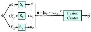
Figure 1: System Model for Distributed Estimation.

II-B Problem formulation

To evaluate the estimation performance, we define a $\operatorname{cost}$ function $C_{\theta}\left(\hat{\theta},\mathbf{u}\right)$ for the desired parameter $\theta$, and a widely adopted one is based on the MSE principle, i.e.,

$$C_{\theta}\left(\hat{\theta},\mathbf{u}\right)=\mathbb{E}_{\theta,\mathbf{u}}[|\theta-\hat{\theta}\left(\mathbf{u}\right)|^{2}].$$ (2)

The optimal quantizers $\{p(u_{k}|X_{k})\}_{k=1}^{K}$ and FC $\hat{\theta}(\mathbf{u})$ are chosen to minimize $C_{\theta}\left(\hat{\theta},\mathbf{u}\right)$, and the corresponding MSE minimization problem is formulated as

$$\underset{\left\{p(u_{k}|X_{k})\right\}_{k=1}^{K},\,\hat{\theta}(\cdot)}{\min}\ C_{\theta}\left(\hat{\theta},\mathbf{u}\right).$$ (3)

Problem (3) is applied for various types of quantizer designs at the sensors, including the deterministic threshold quantizer and the quantizer with random dithering [30].

For the scenario where all sensors have conditionally i.i.d. local observations and identical quantization level $L$, it was demonstrated in [28] that adopting identical quantizer across all the sensors, i.e.,

$$p(u_{i}=u|X_{i}=x)=p(u_{j}=u|X_{j}=x),$$ (4)

$\forall i,j\in[K],u\in\{0,1,\cdots,L-1\},x\in\mathbb{R}$, can achieve the global optima for problem (3). Then, we can further prove the conditionally i.i.d. property for the quantized data from all sensors.

Proposition II.1

If all sensors have conditionally i.i.d. local observations and adopt identical quantizer, then the quantized data $\{u_{k}\}_{k=1}^{K}$ are conditionally i.i.d. with given $\theta$. In other words, we have $p(\mathbf{u}|\theta)=\prod_{k=1}^{K}p(u_{k}|\theta)$ and $p(u_{i}=u|\theta)=p(u_{j}=u|\theta)$, $\forall i,j\in[K],u\in\{0,1\cdots,L-1\}$.

Proof:

By subsisting (1) and (4) into $p(u|\theta)=\int_{x}p(u|X=x)f_{X}(x|\theta)$ and $p(\mathbf{u}|\theta)=\prod_{k=1}^{K}p(u_{k}|\theta)$, Proposition II.1 is proved. ∎

Therefore, we ignore the indices of the sensors in the sequel, and problem (3) can be simplified as

$$\underset{p(u|X),\,\hat{\theta}(\cdot)}{\min}\ C_{\theta}\left(\hat{\theta},\mathbf{u}\right).$$ (5)

III Binary Quantization Scheme

This section considers the design of identical binary probabilistic quantizer at all sensors. First, the MSE lower bound for the binary-quantization-based distributed estimation is derived to serve as the benchmark for the quantization performance evaluation, and the binary probabilistic quantizer is designed to minimize this lower bound. Then, the optimality of the mean-fusion operation at the FC is proved, and the corresponding FC design is derived. Finally, a joint model and data driven method is proposed to sequentially train the design parameters of both the quantizer and FC modules.

III-A MSE lower bound and optimality of mean-Fusion

Considering the use of identical binary quantizer with $L=2$ at all sensors, i.e., $u_{1},\cdots,u_{K}\in\{0,1\}$, the following proposition gives the achievable MSE lower bound for the binary-quantization-based distributed estimation of $\theta$ at the FC.

Proposition III.1

When the binary quantized data $u_{1},\cdots,u_{K}$ from all sensors are conditionally i.i.d. with given $\theta$, the MSE for estimating $\theta$ using $\theta$ is lower bounded by

$$\mathbb{E}[|\theta-\hat{\theta}(\mathbf{u})|^{2}]\geq\mathcal{L}_{binary}^{K}(\gamma),$$ (6)

where

$$\mathcal{L}_{binary}^{K}(\gamma)=\mathbb{E}[\theta^{2}]-\sum_{k=0}^{K}C_{K}^{k}\frac{\mathbb{E}_{\theta}^{2}\left[\theta\gamma(\theta)^{k}(1-\gamma(\theta))^{K-k}\right]}{\mathbb{E}_{\theta}\left[\gamma(\theta)^{k}(1-\gamma(\theta))^{K-k}\right]}$$ (7)

is the MSE lower bound, and

$$\gamma(\theta)=p(u=1|\theta)=\mathbb{E}_{X}[p(u=1|X)|\theta]$$ (8)

denotes the noisy quantization probability for any quantized data $u$ being "1" with given $\theta$. The equality in (6) holds if and only if $\hat{\theta}(\mathbf{u})=\mathbb{E}_{\theta}\left[\theta p\left(\mathbf{u}\left|\theta\right.\right)\right]/\mathbb{E}_{\theta}\left[p\left(\mathbf{u}\left|\theta\right.\right)\right]$.

Proof:

See Appendix A for details. ∎

Remark III.1

It is observed from (7) that $\mathcal{L}_{binary}^{K}(\gamma)$ is determined by the conditional probability distribution of the quantized data with given $\theta$, i.e., $p(u=1|\theta)=\gamma(\theta)$ and $p(u=0|\theta)=1-\gamma(\theta)$. With the MMSE criterion, the achievable MSE lower bound $\mathcal{L}_{binary}^{K}(\gamma)$ serves as the benchmark for the quantization performance evaluation at the sensors, and the optimal quantizer is designed to minimize $\mathcal{L}_{binary}^{K}(\gamma)$.

Proposition III.1 established a design metric for the quantizer by minimizing the MSE lower bound. Moreover, by demonstrating the optimality of mean-fusion operation at the FC with conditionally i.i.d. quantized data, the estimation design problem at the FC can be further simplified.

Proposition III.2

If the binary quantized data $u_{k}$, $k=1,\cdots,K$, from all sensors are conditionally i.i.d. with given $\theta$, then the quantized data $\mathbf{u}=[u_{1},\dots,u_{K}]^{T}$ and their average $\bar{u}=\frac{1}{K}\sum_{k=1}^{K}u_{k}$ own identical Fisher Information for any given $\theta$, i.e.,

$$\mathbb{E}_{\mathbf{u}}\left[\frac{\partial^{2}\ln p(\mathbf{u}\mid\theta)}{\partial\theta^{2}}\right]=\mathbb{E}_{\bar{u}}\left[\frac{\partial^{2}\ln p(\bar{u}\mid\theta)}{\partial\theta^{2}}\right].$$ (9)

Furthermore, estimations of $\theta$ by using $\mathbf{u}$ and $\bar{u}$ can achieve identical MSE lower bound, i.e.,

$$\mathbb{E}[|\theta-\hat{\theta}(\bar{u})|^{2}]\geq\mathcal{L}_{binary}^{K}(\gamma).$$ (10)

where $\mathcal{L}_{binary}^{K}(\gamma)$ is given in (7) as the lower bound for estimation using $\mathbf{u}$. The equality in (10) holds if and only if $\hat{\theta}(\bar{u})=\mathbb{E}_{\theta}\left[\theta p\left(\bar{u}\left|\theta\right.\right)\right]/\mathbb{E}_{\theta}\left[p\left(\bar{u}\left|\theta\right.\right)\right]$.

Proof:

See Appendix B for details. ∎

Remark III.2

According to the reciprocity of the estimation MSE and Fisher information [28], i.e., higher Fisher information implies lower MSE and vice versa, both (9) and (10) indicate that the achievable minimum MSE for estimating $\theta$ with either $\mathbf{u}$ or $\bar{u}$ is equivalent. The employment of original quantized data $\mathbf{u}$ for estimation in FC renders its input dimension susceptible to changes in the number of sensors. Therefore, when the designed FC cannot adopt to fluctuations in the number of sensors, the performance is likely to deteriorate. The mean-fusion operation enables the FC to use $\bar{u}$ with fixed input dimension and robustly serve the system with dynamical number of sensors in the network.

III-B Design of probabilistic quantizer and fusion center

According to Remarks III.1 and III.2, we are motivated to implement the binary probabilistic quantizer with random dithering and the FC with mean-fusion operation.

III-B1 Probabilistic quantizer

As shown in Fig. 2, we consider one implementation of the binary probabilistic quantizer design with random dithering. Define the probability controller $G(\cdot):\mathbb{R}\rightarrow[0,1]$. The local observation $X$ is first sent to $G(\cdot)$, and the output $G(X)$ is then fed into the quantization function $Q(\cdot):[0,1]\rightarrow\{0,1\}$ to generate a random binary data

$$u=Q(G(X))=\frac{1+\mathrm{sgn}(G(X)-z)}{2}\in\{0,1\},$$ (11)

where $z\sim\mathrm{U}(0,1)$ is a standard uniform distributed dithering noise, and $\mathrm{sgn}(\cdot)$ is the sign function.

It is observed from $\eqref{eq: probabilistic quantization 1}$ that the probability of the local observation $X$ being quantized as $u=1$ is equal to $G(X)$, i.e.,

$$p(u=1|X)= p\left(\frac{1+\mathrm{sgn}(G(X)-z)}{2}=1\Big{|}X\right)$$ (12)

$$= p(G(X)>z|X)$$

$$= G(X),$$

and intuitively we have $p(u=0|X)=1-G(X)$. Therefore, by using Proposition III.1 and (12), to minimize the MSE lower bound $\mathcal{L}_{binary}^{K}(\gamma)$ in (7) is equivalent to find the optimal probability controller $G(\cdot)$ for the quantizer, i.e.,

$$\underset{G(\cdot)}{\min}\quad\mathcal{L}_{binary}^{K}(\gamma),$$ (13)

where $\gamma(\theta)$ defined in (8) is rewritten as

$$\begin{split}\gamma(\theta)=\mathbb{E}_{X}[G(X)|\theta].\end{split}$$ (14)

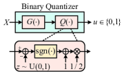
Figure 2: Binary probabilistic quantizer

$$\underset{\Phi}{\min}\ \ \mathcal{L}_{binary}^{K}(\Phi)=\mathbb{E}[\theta^{2}]-\sum_{k=0}^{K}C_{K}^{k}\left({\mathbb{E}_{\theta}^{2}\left[\theta\left(\gamma_{\Phi}(\theta)\right)^{k}\left(1-\gamma_{\Phi}(\theta)\right)^{K-k}\right]}\right)/\left({\mathbb{E}_{\theta}\left[\left(\gamma_{\Phi}(\theta)\right)^{k}\left(1-\gamma_{\Phi}(\theta)\right)^{K-k}\right]}\right),$$ (19)

$$\underset{\{\Phi,\Psi\}}{\min}\ \mathcal{T}_{binary}^{K}(\Phi,\Psi)=\sum_{k=0}^{K}C_{K}^{k}\mathbb{E}_{\theta}\left[\left|\theta-F_{\Psi}\left(\bar{u}=\frac{k}{K}\right)\right|^{2}(\gamma_{\Phi}(\theta))^{k}\left(1-\gamma_{\Phi}(\theta)\right)^{K-k}\right].$$ (20)

III-B2 Fusion center

As shown in Fig 3, we are motivated by Remark III.2 to implement a FC with mean-fusion operation. After the binary quantized data $\{u_{k}\}_{k=1}^{K}$ from all sensors are received by the FC, they are first averaged to get $\bar{u}=\frac{1}{K}\sum_{k=1}^{K}u_{k}$. Then, the desired parameter $\theta$ is estimated as

$$\hat{\theta}=F(\bar{u}),$$ (15)

where $F(\cdot){:[0,1]\rightarrow\mathbb{R}}$ is the estimator function to be designed. From (15) and by using

$$p\left(\bar{u}=\frac{k}{K}\big{|}\theta\right)=C_{K}^{k}\left(\gamma(\theta)\right)^{k}\left(1-\gamma(\theta)\right)^{K-k},$$

which is derived in (49), the estimation MSE for $\theta$ at the FC is computed as

$$\mathcal{T}_{binary}^{K}(F)= \ \mathbb{E}_{\theta,\bar{u}}[|\theta-F(\bar{u})|^{2}]$$ (16)

$$= \mathbb{E}_{\theta}\left[\sum_{k=0}^{K}\left|\theta-F\left(\frac{k}{K}\right)\right|^{2}p\left(\bar{u}=\frac{k}{K}\bigg{|}\theta\right)\right]$$

$$= \sum_{k=0}^{K}C_{K}^{k}\mathbb{E}_{\theta}\left[\left|\theta-F\left(\frac{k}{K}\right)\right|^{2}\gamma(\theta)^{k}\left(1-\gamma(\theta)\right)^{K-k}\right].$$

For the goal to minimize the estimation MSE in (16), the best estimator function for FC is designed as

$$\underset{F(\cdot)}{\min}\ \mathcal{T}_{binary}^{K}(F).$$ (17)

Remark III.3

If perfect statistic knowledge on the distributions of the desired parameter and noise is available, problems (13) and (17) are variational problems of $G(\cdot)$ and $F(\cdot)$, which can be solved by calculus of variations under certain conditions [28]. The non-closed-form solution of $G(\cdot)$ can also be obtained based on the parametric and data driven method with data samples generated from the respective distributions[27]. Since perfect information about the distributions of the desired parameter and observation noise is difficult to be obtained in practical systems, it is more interesting to study the scenarios that both the above distributions are unknown or only the noise distribution is known. Thus, a joint model and data driven method is proposed as shown in the next subsection.

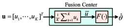
Figure 3: Mean-fusion operation for binary-quantization-based distributed estimation.

III-C Joint model and data driven method

A joint model and data driven method to solve problems (13) and (17) is proposed in the following:

III-C1 Binary quantizer

For the binary probabilistic quantizer defined in Fig. 2, its probability controller $G(\cdot)$ is implemented as a DNN $G_{\Phi}$ with $N$ fully connected layers (FCLs)[31]. In the DNN $G_{\Phi}$ as shown in Fig. 4(a), the input observation $X$ is fed into $N$ FCLs, i.e.,

$$G_{\Phi}(X)=g_{N}\circ\cdots\circ g_{2}\circ g_{1}(X),$$ (18)

where $g_{i}$, $i\in[N]$, is the FCL with the parameter $\alpha_{N}$, the number of input dimensions being $L_{g,I,i}$, and the number of output dimensions being $L_{g,O,i}$. Note that $L_{g,I,1}=L_{g,O,N}=1$ is fixed. To mitigate the issues of gradient explosion and vanishing, the ReLU function [31] is employed as the activation function for $g_{1},g_{2},\cdots,g_{N-1}$. In the output layer $g_{N}$, the Sigmoid function is utilized as the activation function to ensure the output range is confined to $[0,1]$, as it represents the quantization probability. To summarize, the training parameter of $G_{\Phi}$ is $\Phi=\{\alpha_{1},\alpha_{2},\cdots,\alpha_{N}\}$.

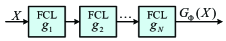
(a) Probability controller DNN

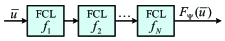
(b) Estimator DNN

Figure 4: Architecture of the probability controller and estimator DNNs.

III-C2 FC

For the FC defined in Fig. 3, its estimator function $F(\cdot)$ is implemented as a DNN $F_{\Psi}$ with $N$ FCLs, denoted as $f_{1},f_{2},\cdots,f_{N}$. Similarly, the ReLU function is employed as the activation function for $f_{1},f_{2},\cdots,f_{N-1}$ to address gradient-related challenges. In the output layer $f_{N}$, the Tanh function is utilized as the activation function, as it ensures the output of $F_{\Psi}$ represents a normalized estimator within the range of $[-1,1]$. The training parameter of $F_{\Psi}$ is denoted as $\Psi=\{\beta_{1},\beta_{2},\cdots,\beta_{N}\}$, where $\beta_{i}$ is the parameter of the FCL $f_{i}$, $i\in[N]$. $L_{f,I,i}$ and $L_{f,O,i}$ are the numbers of input dimensions and output dimensions of the FCL $f_{i}$, $i\in[N]$, with $L_{f,I,1}=L_{f,O,N}=1$ being fixed.

Then, by adopting the DNNs, optimization problems (13) and (17) are rewritten as (19) and (20).

Remark III.4

Based on the MMSE criterion, problems (19) and (20) imply that the optimal quantizer design is independent of the FC design and the optimal FC design is obtained based on the optimal quantizer. For the practical scenario that the quantizer and FC are separated in space, the regular joint training method of the two modules a sequential deep learning training method to obtain optimal $G_{\Phi}$ and $F_{\Psi}$ is proposed in the next subsection. Notice that the sequential training

III-D Sequential training method

For the sequential training of the probability controller DNN $G_{\Phi}$ in quantizer and estimator DNN $F_{\Psi}$ in FC, we aim to first find the optimal parameter $\Phi^{*}$ which minimizes the loss function $\mathcal{L}_{binary}^{K}(\Phi)$ in (19), and then find the optimal $\Psi^{*}$ that minimizes the loss function $\mathcal{T}_{binary}^{K}(\Phi^{*},\Psi)$ in (20), under two cases that the distributions of both the desired parameter and observation noise are unknown or only the noise distribution is known. Besides, it is observed that the two loss functions are contingent upon the number of sensors $K$. Given the consideration of a practical network where the number of sensors may vary dynamically, a predetermined number of sensors is chosen during the training phase, while the efficacy of the trained model is assessed using varying sensor quantities during the testing phase.

III-D1 Training with unknown parameter and noise distributions

The training process is based on the data set $D_{1}=\{\theta_{t},\mathbf{x}_{t}\}_{t=1}^{T}$, where $\theta_{t}$ is the $t$-th sample of the desired parameter $\theta$ to be estimated, $\mathbf{x}_{t}=\{x_{t,1},\cdots,x_{t,Q}\}$ contains $Q$ noise-corrupted observation samples of $\theta_{t}$, and $T$ denotes the total number of training samples. The desired parameter $\theta_{t}$ is obtained from the experimental environment, and the observation $x_{t,1},\cdots,x_{t,Q}$ are obtained from the sensor by periodically observing $\theta_{t}$ under the same environment.

At each epoch, based on the mini batch method[31], the whole data set is divided into $T/B$ batches where $B$ is the number of batch samples. Here, we consider the case that $T/B$ is an integer, without loss of generality. In the exceptional scenario, a simple approach is to randomly select additional samples from the existing dataset and append them to form a new dataset that satisfies the requirement. Parameter $\Phi$ is trained for $T/B$ times within an epoch, where each time a new batch set is utilized for training. Within each time, the loss function in (19) is approximated and averaged on the whole batch samples as

$$\hat{\mathcal{L}}_{1}=\sum_{t=1}^{B}(\theta_{t})^{2}-\sum_{k=0}^{K_{S}}C_{K_{S}}^{k}\frac{\left(\sum_{t=1}^{B}\theta_{t}\left(\gamma_{\Phi}^{t}\right)^{K_{S}}\left(1-\gamma_{\Phi}^{t}\right)^{{K_{S}}-k}\right)^{2}}{\sum_{t=1}^{B}\left(\gamma_{\Phi}^{t}\right)^{K_{S}}\left(1-\gamma_{\Phi}^{t}\right)^{{K_{S}}-k}},$$ (21)

where $K_{S}$ is the predetermined sensor quantity parameter in the training and

$$\gamma_{\Phi}^{t}=\sum_{q=1}^{Q}G_{\Phi}(x_{t,q})$$ (22)

is the empirical approximation of $\gamma_{\Phi}(\theta_{t})=\mathbb{E}_{X}[G_{\Phi}(X)|\theta_{t}]$ over data set $\{\theta_{t},\mathbf{x}_{t}\}$. By using the back propagation algorithm[31], the gradient $\nabla_{\Phi}\hat{\mathcal{L}_{1}}$ is calculated based on (21), and the parameter $\Phi$ is updated epoch by epoch. After the maximum number of training epochs is reached, the optimal parameter is obtained as $\Phi^{*}$.

Once the optimal probability controller $G_{\Phi^{*}}$ in the quantizer is obtained, it is utilized to sequentially train the estimator DNN $F_{\Psi}$ in the FC. The training of $F_{\Psi}$ uses the same mini batch method based on data set $D_{1}$. Within each time, the loss function in (20) is approximated and averaged on the whole batch samples as

$$\hat{\mathcal{T}}_{1}= \sum_{t=1}^{B}\sum_{k=0}^{K_{F}}\left(\theta_{t}-F_{\Psi}\left(\frac{k}{K_{F}}\right)\right)^{2}C_{K_{F}}^{k}\left(\gamma_{t}^{*}\right)^{k}\left(1-\gamma_{t}^{*}\right)^{{K_{F}}-k},$$ (23)

where $K_{F}$ is the predetermined sensor quantity parameter in the training and

$$\gamma_{t}^{*}=\sum_{q=1}^{Q}G_{\Phi^{*}}(x_{t,q}).$$ (24)

Based on (23), parameter $\Psi$ is updated epoch by epoch using the back propagation algorithm[31], and optimal $\Psi^{*}$ is obtained once the maximum training epochs are reached.

III-D2 Training with known noise distribution

If the statistic information about the distribution of the observation noise is available, then intuitively $f_{X}({\cdot|\theta})$ is obtained and we can use only data set $D_{2}=\{\theta_{t}\}_{t=1}^{T}$ for the sequential training. Considering the case that the sensor’s observation range is restricted to $[-W,W]$, we define an artificial observation set $O=\{-W,-\frac{Q-1}{Q}W,\cdots,0,\frac{1}{Q}W,\cdots,W\}$ to cover the bounded observations. Based on the information of distribution $f_{X}(\cdot|\theta)$, the loss function $\mathcal{L}_{binary}^{K}(\Phi)$ in (19) is approximated based on the whole batch samples as

$$\hat{\mathcal{L}}_{2}=\sum_{t=1}^{B}(\theta_{t})^{2}-\sum_{k=0}^{K_{S}}C_{K_{S}}^{k}\frac{\left(\sum_{t=1}^{B}\theta_{t}\left(\gamma_{\Phi}^{t}\right)^{k}\left(1-\gamma_{\Phi}^{t}\right)^{{K_{S}}-k}\right)^{2}}{\sum_{t=1}^{B}\left(\gamma_{\Phi}^{t}\right)^{k}\left(1-\gamma_{\Phi}^{t}\right)^{{K_{S}}-k}},$$ (25)

where $\gamma_{\Phi}^{t}=\sum_{x\in O}G_{\Phi}(x)f_{X}(x|\theta_{t})$. By using the back propagation algorithm, parameter $\Phi$ is updated epoch by epoch based on (25), and optimal $\Phi^{*}$ is obtained after the maximum number of training epochs is reached.

With the optimal probability controller $G_{\Phi^{*}}$, the estimator DNN $F_{\Psi}$ in the FC is sequentially trained. The training of FC utilizes the same mini batch method based on the sets $D_{2}$ and $O$. Within each time, the loss function in (20) is approximated and averaged on the whole batch samples as

$$\hat{\mathcal{T}}_{2}= \sum_{t=1}^{B}\sum_{k=0}^{K_{F}}\left(\theta_{t}-F_{\Psi}\left(\frac{k}{K_{F}}\right)\right)^{2}C_{K_{F}}^{k}\left(\gamma_{t}^{*}\right)^{K_{F}}\left(1-\gamma_{t}^{*}\right)^{{K_{F}}-k},$$ (26)

where $\gamma_{t}^{*}=\sum_{x\in O}G_{\Phi^{*}}(x)f_{X}(x|\theta_{t})$. Based on (26), optimal parameter $\Psi^{*}$ is obtained by updating $\Psi$ epoch by epoch using the back propagation algorithm until the maximum number of training epochs are reached.

Finally, the performance of the proposed sequential training scheme is compared with an canonical alternative training scheme, in which a total of 500 epochs are divided into 10 rounds, and the quantizer and FC DNNs are trained alternately for each round. Figure 5 illustrates the plotted MSE loss of both the quantizer and FC with respect to the training epochs. Notably, the proposed sequential training scheme demonstrates superior and smoother convergence during the training phase. Additionally, the final MSE loss achieved by the sequential training scheme is smaller compared to that of the alternated training approach. This strongly supports the effectiveness of the proposed sequential training method.

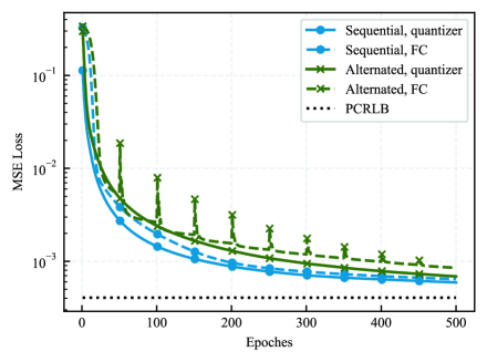
Figure 5: Convergence of the quantizer and FC training.

$$\mathcal{T}_{\mathrm{parallel}}^{M,K}(\Phi,\Psi)=\mathbb{E}_{\theta}\left[\sum_{\bar{\mathbf{u}}}\left|\theta-F_{\Psi}\left(\bar{\mathbf{u}}\right)\right|^{2}p\left(\bar{\mathbf{u}}|\theta\right)\right]=\sum_{i_{1}=0}^{K}\cdots\sum_{i_{M}=0}^{K}\mathbb{E}_{\theta}\left[\left|\theta-F_{\Psi}\left(\frac{i_{1},\cdots,i_{M}}{K}\right)\right|^{2}p_{\Phi}^{i_{1},\cdots,i_{M}}(\theta)\right].$$ (33)

IV Multi-bit Probabilistic Quantization

In this section, we relax the assumption of one-bit quantization constraint at sensors and address the optimal design of multi-bit probabilistic quantizer and FC. We consider two different joint model and data driven multi-bit quantization schemes, corresponding to parallel and one-hot implementation of quantization for all bits in a multi-bit quantized information. Owing to the similarities in the optimization of the multi-bit quantizer and FC design with that under the binary quantization constraint discussed in Section III, we omit the details of the deep learning training process for the quantizer and FC in this section.

IV-A Parallel quantization

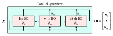
(a) Quantizer

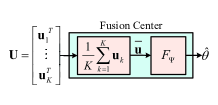
(b) FC

Figure 6: Multi-bit parallel quantization and mean-vector-fusion.

The joint model and data driven multi-bit parallel quantizer and FC modules are shown in Fig. 6:

• Quantizer: As shown in Fig. 6(a), we consider an $M$-bit parallel quantizer module where the quantization is implemented by $M$ parallel binary quantizers (BQ). Each BQ adopts identical binary quantizer design shown in Fig. 2. Taking the $m$-th BQ as an example, it maps the input observation $X$ into a binary output $u_{m}\in\{0,1\}$ following the distribution $p(u_{m}=1|X)=G_{\phi_{m}}(X)$ and $p(u_{m}=0|X)=1-G_{\phi_{m}}(X)\}$, where $G_{\phi_{m}}$ is the probability controller DNN in the $m$-th BQ with design parameter $\phi_{m}$. Thus, $M$ BQs map the observation as an $M$-bit quantization message $\mathbf{u}=[u_{1},u_{2},\cdots,u_{M}]^{T}\in\{0,1\}^{M}$.

• FC: As shown in Fig. 6(b), we consider the scenario that $K$ sensors adopt identical $M$-bit parallel quantizer with design parameters $\Phi=\{\phi_{1},\cdots,\phi_{m}\}$. The FC receives $K$ quantized messages $\mathbf{U}=[\mathbf{u}_{1},\cdots,\mathbf{u}_{K}]^{T}$ from $K$ sensors and uses the mean-vector-fusion operation to obtain $\bar{\mathbf{u}}=\frac{1}{K}\sum_{k=1}^{K}\mathbf{u}_{k}$. The desired parameter $\theta$ is estimated as

  $$\hat{\theta}=F_{\Psi}(\bar{\mathbf{u}}),$$ (27)

  where $F_{\Psi}(\cdot):[0,1]^{M}\rightarrow\mathbb{R}$ is the estimator DNN with design parameters $\Psi$.

Similar to Proposition III.1, the following proposition shows that if identical multi-bit parallel quantizer is deployed at all sensors, then adopting the mean-vector-fusion operation on the quantized data causes no performance degradation for the estimation of the desired parameter.

Proposition IV.1

If all sensors adopt the identical $M$-bit parallel quantizer with design parameter $\Phi=\{\phi_{1},\cdots,\phi_{m}\}$, estimation of $\theta$ by using the original quantized data matrix $\mathbf{U}$ or only the mean-vector $\bar{\mathbf{u}}$ can achieve identical MSE lower bound, i.e.,

$$\mathbb{E}[|\theta-\hat{\theta}(\mathbf{U})|^{2}]\geq \mathcal{L}_{\mathrm{parallel}}^{M,K}(\Phi),$$ (28)

$$\mathbb{E}[|\theta-\hat{\theta}(\bar{\mathbf{u}})|^{2}]\geq \mathcal{L}_{\mathrm{parallel}}^{M,K}(\Phi),$$ (29)

where

$$\mathcal{L}_{\mathrm{parallel}}^{M,K}(\Phi)=\sum_{i_{1}=0}^{K}\cdots\sum_{i_{M}=0}^{K}\frac{\mathbb{E}_{\theta}^{2}\left[\theta p_{\Phi}^{i_{1},\cdots,i_{M}}(\theta)\right]}{\mathbb{E}_{\theta}\left[p_{\Phi}^{i_{1},\cdots,i_{M}}(\theta)\right]},$$ (30)

is the MSE lower bound,

$$p_{\Phi}^{i_{1},\cdots,i_{M}}(\theta)= p\left(\bar{\mathbf{u}}=\frac{1}{K}[i_{1},\cdots,i_{M}]^{T}\Big{|}\theta\right)$$ (31)

$$= \prod_{m=1}^{M}C_{K}^{i_{m}}(\gamma_{\phi_{m}}(\theta))^{i_{m}}(1-\gamma_{\phi_{m}}(\theta))^{K-i_{m}},$$

and

$$\gamma_{\phi_{m}}(\theta)=p([\mathbf{u}]_{m}=1|\theta)=\mathbb{E}_{X}[G_{\phi_{m}}(X)|\theta]$$ (32)

denotes the conditional probability for the $m$-th bit of any quantized vector being "$1$" with given $\theta$. The equality in (28) holds if and only if $\hat{\theta}(\mathbf{U})=\mathbb{E}_{\theta}\left[\theta p\left(\mathbf{U}\left|\theta\right.\right)\right]/\mathbb{E}_{\theta}\left[p\left(\mathbf{U}\left|\theta\right.\right)\right]$, and the equality in (29) holds if and only if $\hat{\theta}(\bar{\mathbf{u}})=\mathbb{E}_{\theta}\left[\theta p\left(\bar{\mathbf{u}}\left|\theta\right.\right)\right]/\mathbb{E}_{\theta}\left[p\left(\bar{\mathbf{u}}\left|\theta\right.\right)\right]$.

Proof:

See Appendix C for details. ∎

By using (27) and (32) and following the analysis in (16), the estimation MSE for $\theta$ at the FC is computed as (33). From (30) and (33), the optimization problems for the multi-bit parallel quantizer and FC are derived as

$$\underset{\Phi}{\min}\ \mathcal{L}_{\mathrm{parallel}}^{M,K}(\Phi),$$ (34)

$$\underset{\{\Phi,\Psi\}}{\min}\ \mathcal{T}_{\mathrm{parallel}}^{M,K}(\Phi,\Psi).$$ (35)

Since the deep learning based training for $\Phi$ and $\Psi$ is similar to that for the binary quantization scenario discussed in section III-D, we ignore the details of the training process.

$$\mathcal{L}_{\mathrm{onehot}}^{M,K}(\Phi)=\mathbb{E}[\theta^{2}]-\sum_{i_{0}=0}^{K}\cdots\sum_{i_{k}=0}^{K-\sum\limits_{l=0}^{k-1}i_{l}}\cdots\sum_{i_{L-2}=0}^{K-\sum\limits_{l=0}^{L-3}i_{l}}\left({\mathbb{E}_{\theta}^{2}\left[\theta q_{\Phi}^{i_{0},\cdots,i_{L-1}}(\theta)\right]}\right)/\left({\mathbb{E}_{\theta}\left[q_{\Phi}^{i_{0},\cdots,i_{L-1}}(\theta)\right]}\right),$$ (39)

$$\mathcal{T}_{\mathrm{onehot}}^{M,K}(\Phi,\Psi)=\mathbb{E}_{\theta}\left[\sum_{\bar{\mathbf{v}}}\left|\theta-F_{\Psi}\left(\bar{\mathbf{v}}\right)\right|^{2}p\left(\bar{\mathbf{v}}|\theta\right)\right]=\sum_{i_{0}=0}^{K}\cdots\sum_{i_{k}=0}^{K-\sum\limits_{l=0}^{k-1}i_{l}}\cdots\sum_{i_{L-2}=0}^{K-\sum\limits_{l=0}^{L-3}i_{l}}\mathbb{E}_{\theta}\left[\left|\theta-F_{\Psi}\left(\frac{i_{0},\cdots,i_{L-1}}{K}\right)\right|^{2}q_{\Phi}^{i_{0},\cdots,i_{L-1}}(\theta)\right].$$ (41)

IV-B One-hot quantization

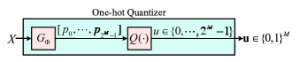
(a) Quantizer

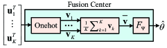
(b) FC

Figure 7: Multi-bit one-hot quantization and mean-one-hot-vector fusion.

The joint model and data driven multi-bit one-hot quantizer and FC modules are shown in Fig. 7:

• Quantizer: As shown in Fig. 7(a), we consider an $M$-bit one-hot quantization module where the probability distribution of the $M$-bit quantized data is controlled by an one-hot probability controller DNN $G_{\Phi}(\cdot):\mathbb{R}\rightarrow[0,1]^{2^{M}}$ with softmax output and design parameter $\Phi$. Local observation $X$ is first sent to $G_{\Phi}$ and mapped as a $2^{M}$-dimensional probability vector $\mathbf{p}=[p_{0},\cdots,p_{2^{M}-1}]^{T}=G_{\Phi}(X)$, where $0\leq p_{m}\leq 1$ and $\sum_{m=0}^{2^{M}-1}p_{m}=1$. Then, the probability vector $\mathbf{p}$ is fed into the quantization function $Q(\cdot):[0,1]^{2^{M}}\rightarrow\{0,1,\cdots,2^{M}-1\}$ to generate a quantized value $u=Q(\mathbf{p})$. Similar to the quantization function $Q(\cdot)$ in binary quantizer, function $Q(\cdot)$ in $M$-bit one-hot quantizer is to make the probability distribution $\{p(u=m|X)\}_{m=0}^{2^{M}-1}$ being controlled by the probability vector $\mathbf{p}$, i.e.,

  $$p(u=m|X)=p(Q(\mathbf{p})=m|X)=p_{m}=[G_{\Phi}(X)]_{m},$$ (36)

  for $m=0,1,\cdots,2^{M}-1$, where $[G_{\Phi}(X)]_{m}$ is the $m$-th entry of vector $G_{\Phi}(X)$. Then, the quantized value $u$ is transformed into a corresponding binary vector $\mathbf{u}\in\{0,1\}^{M}$, which is then being transmitted to the FC.

• FC: As shown in Fig. 7(b), we consider the scenario that $K$ sensors adopt the identical $M$-bit one-hot quantizer with design parameter $\Phi$. The FC receives $K$ quantized messages $\mathbf{U}=[\mathbf{u}_{1},\cdots,\mathbf{u}_{K}]^{T}$ from $K$ sensors and transforms them into $K$ one-hot vectors as $\mathbf{V}=[\mathbf{v}_{1},\cdots,\mathbf{v}_{K}]^{T}$. Based on the one-hot encoding scheme [31], each vector $\mathbf{u}_{k}\in\{0,1\}^{M}$ is transformed as a $2^{M}$-dimensional vector

  $$\mathbf{v}_{k}=\begin{cases}[1,\mathbf{0}_{2^{M}-1}^{T}]^{T},&(\mathbf{u}_{k})_{10}=0,\\ [\mathbf{0}_{(\mathbf{u}_{k})_{10}}^{T},1,\mathbf{0}_{2^{M}-(\mathbf{u}_{k})_{10}-1}^{T}]^{T},&(\mathbf{u}_{k})_{10}\geq 1,\\ \end{cases}$$

  where $\mathbf{0}_{2^{M}-1}^{T}$ is $(2^{M}-1)$-dimensional zero vector and $(\mathbf{u}_{k})_{10}$ is the decimal expression of $\mathbf{u}_{k}$. Then, the mean-one-hot-vector $\bar{\mathbf{v}}=\frac{1}{K}\sum_{k=1}^{K}\mathbf{v}_{k}$ is utilized to estimate the desired parameter $\theta$ as $\hat{\theta}=F_{\Psi}(\bar{\mathbf{v}})$, where $F_{\Psi}(\cdot):[0,1]^{2^{M}}\rightarrow\mathbb{R}$ is the estimator DNN with design parameter $\Psi$.

The following proposition shows that if identical multi-bit one-hot quantizer is deployed at all sensors, then adopting the mean-one-hot-vector-fusion operation on the quantized data causes no performance degradation for the estimation of the desired parameter.

Proposition IV.2

If all sensors adopt the identical $M$-bit one-hot quantizer with design parameter $\Phi$, estimation of $\theta$ by using the original quantized data matrix $\mathbf{U}$ or only the mean-one-hot-vector $\bar{\mathbf{v}}$ can achieve identical MSE lower bound, i.e.,

$$\mathbb{E}[|\theta-\hat{\theta}(\mathbf{U})|^{2}]\geq\mathcal{L}_{\mathrm{onehot}}^{M,K}(\Phi),$$ (37)

$$\mathbb{E}[|\theta-\hat{\theta}(\bar{\mathbf{v}})|^{2}]\geq\mathcal{L}_{\mathrm{onehot}}^{M,K}(\Phi),$$ (38)

where $\mathcal{L}_{\mathrm{onehot}}^{M,K}(\Phi)$ in (39) is the MSE lower bound, $L=2^{M}$, $i_{L-1}=K-\sum_{l=0}^{L-2}i_{l}$,

$$q_{\Phi}^{i_{0},\cdots,i_{L-1}}(\theta)=\prod_{l=0}^{L-2}C_{K-i_{0}\cdots-i_{l-1}}^{i_{l}}(\gamma_{\Phi,l}(\theta))^{i_{l}},$$ (40)

and,

$$\gamma_{\Phi,l}(\theta)=\mathbb{E}_{X}[[G_{\Phi}(X)]_{l}|\theta].$$

Proof:

See Appendix D for details. ∎

By using (40) and following the analysis in (16), the estimation MSE for $\theta$ at the FC is computed as (41). From (39) and (41), the optimization problems for the multi-bit one-hot quantizer and FC are derived as

$$\underset{\Phi}{\min}\ \mathcal{L}_{\mathrm{onehot}}^{M,K}(\Phi),$$ (42)

$$\underset{\{\Phi,\Psi\}}{\min}\ \mathcal{T}_{\mathrm{onehot}}^{M,K}(\Phi,\Psi).$$ (43)

Since the training for $\Phi$ and $\Psi$ based on deep learning is similar to the binary quantization scenario discussed in section III-D, we omit the details of training process.

V Simulation Results

This section presents some simulations to validate the proposed method, and the corresponding simulation environment is specified as follows: Initially, the samples of the desired parameter in both the data and test sets are obtained from an uniform distribution over the interval $[-1,1]$ [28]. The observation samples from each sensor are contaminated by i.i.d. Gaussian noise with variance $\sigma^{2}$, and $f_{X}(\cdot|\theta)\sim\mathcal{N}(0,\sigma^{2})$ denotes the conditional distribution of the observation $X$ with given desired parameter $\theta$. The observation signal-to-noise ratio (SNR) in the simulation is defined as the power ratio of the desired parameter to the observation noise.

For the quantizer module, the number of FCLs in the probability controller DNN $G_{\Phi}$ is set as $N=3$, with the number of neurons in each FCL being $L_{G}=20$; for the estimator DNN $F_{\Psi}$ in FC module, the number of neurons in each FCL is set as $L_{F}=30$. $G_{\Phi}$ is trained by a data set of 50000 samples over 500 epochs, with the predetermined sensor quantity parameter in the training of $G_{\Phi}$ being $K_{S}$. Using the trained $G_{\Phi^{*}}$, $F_{\Psi}$ is then trained by the same data set over 500 epochs, with the predetermined sensor quantity parameter in the training of $F_{\Psi}$ being $K_{F}$. Based on the pretest simulation, the maximum epoch number of 500 is deemed efficient enough to achieve the desired convergence of the model training under all scenarios. Besides, to ensure consistency throughout the simulation, the default values for both $K_{S}$ and $K_{F}$ are set to 250. However, it is important to note that certain figures explicitly indicate the usage of different values for $K_{S}$ or $K_{F}$. After the sequential training of $G_{\Phi}$ and $F_{\Psi}$, the entire trained system undergoes validation using an independent test set comprising 10,000 samples. The test set is generated separately from the training set, ensuring a rigorous evaluation of the system’s performance and verifying that our model is not overfitted. The whole training uses the ADMM optimizer[31] with a constant learning rate $l_{r}=0.001$. The implementation of the whole simulations is carried out using PyTorch 1.7.0[31] on an NVIDIA 2080 Super Max-Q GPU. Under the aforementioned simulation environment, the training duration for the complete system is approximately 2 hours for the binary model, 4 hours for the 2-bit parallel models, and 10 hours for the 2-bit one-hot models. In the entire simulations, the DNN parameters are initialized by the widely adopted Kaiming Gaussian distribution method [32], which is the default setting in the Pytorch. Additionally, to ensure the reliability of the results, the simulation of each figure is repeated multiple times to verify their consistency.

For comparisons, we implement the sine-quantization-maximum-likelihood-fusion (SQMLF) method [28], which was proved to be optimal for the estimation of a parameter with uniform distribution under the ideal noiseless scenario. In addition, we also examine the Posterior Cramer-Rao Lower Bound (PCRLB) [26], being the minimum MSE to be achieved by any unbiased estimation method, as the performance limit of the distributed estimation with binary quantization.

V-A Asymptotically optimality and robustness of proposed algorithm

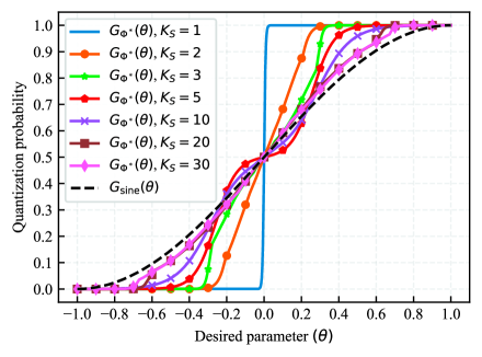
Figure 8: Probability controller $G_{\Phi}$ trained with different $K_{S}$.

First, we study the asymptotic optimality and robustness of the proposed method to the number of sensors. Fig. 8 plots the binary probability controller $G_{\Phi^{*}}$ trained with different $K_{S}$ under the noiseless observation scenario where local observations at sensors equal to the desired parameter. For the estimation of a parameter with uniform distribution under the noiseless scenario, the optimal probability controller function is proved to be $G_{\text{sine}}(\theta)=[1+\sin(\pi\theta/2)]/2$ used in the SQMLF method[26]. Therefore, the closer the trained $G_{\Phi^{*}}$ is to $G_{\text{sine}}$ under the noiseless scenario, the better quantitation performance and estimation performance are expected to be obtained. It is observed that with the increasing of $K_{S}$, the trained $G_{\Phi^{*}}$ gradually approaches to the optimal $G_{\text{sine}}$, which implies the asymptotic optimality of the proposed method.

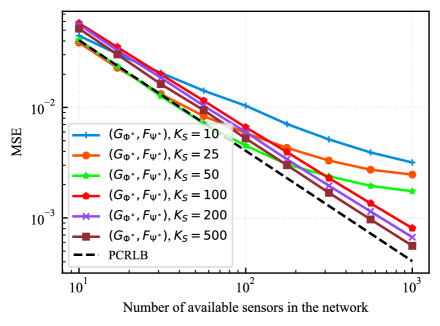
Figure 9: Estimation MSE vs. the number of available sensors in the network.

Fig. 9 plots the estimation MSE of the proposed method as a function of the number of available sensors in the network, with different $K_{S}$ being selected in the training of quantizer. It is observed that selecting bigger $K_{S}$ in training improves the robustness of the proposed method to the variations of the number of sensors in the practical network. For instance, when $K_{S}=10$, although the estimation MSE is close to the PCRLB at the initial phase of the curves, it decreases more slowly and deviates further from the PCRLB as the number of sensors in test increases. While with $K_{S}\geq 100$, the MSE decreases linearly with respect to the number of sensors and remains close to the PCRLB at the whole curves. This validates the robustness of the proposed FC design with mean-fusion operation for accommodating various number of sensors in practice.

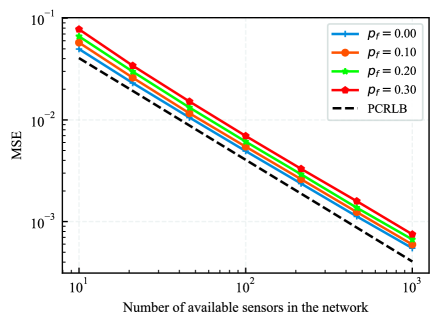
Figure 10: Robustness to the failure of sensors.

To further evaluate the robustness of our method, we conducted additional simulations to assess its performance in scenarios with sudden sensor failures. We consider the situation where each sensor in the network randomly fails to transmit information to the FC with a probability denoted as $p_{f}$. Fig. 10 illustrates the estimation MSE of our method under different values of $p_{f}$. The simulation result reveals a consistent linear decrease in the estimation MSE of our proposed method across varying $p_{f}$ values, as the number of sensors increases. Notably, the MSE remains close to the PCRLB under all conditions. This result provide empirical evidence that our method is robust against sudden sensor failures and possesses a high level of generalization to the network variation.

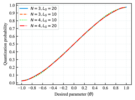
(a) Probability controller DNN $G_{\Phi}$

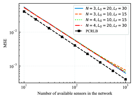
(b) Estimation MSE

Figure 11: Robustness to the neural network initialization.

To investigate the robustness of our method to the neural network initializations, we conducted the simulations of our proposed method with various initial setting parameters, including the number of layers $N$ in the DNNs, the number of neurons $L_{G}$ in each layer of $G_{\Phi}$ and the number of neurons $L_{F}$ in each layer of $F_{\Psi}$. Fig. 11(a) plots the convergence results of the probability controller DNN $G_{\Phi}$ under different numbers of layers and neurons. It is observed that $G_{\Phi}$ converges to almost the same structure despite the variations in DNN setting parameters. Furthermore, Fig. 11(b) portrays the estimation MSE of our method with different numbers of layers and neurons. Similarly, the estimation MSE curves of our method under diverse DNN setting parameters are almost the same, which verify the robustness of our method to the neural network initialization. Besides, it is observed that the minimum DNN initial configuration yielding comparable results for our proposed method is “$N=3,L_{G}=10,L_{F}=15$". As depicted in Fig. 11 our manuscript, a slight increase in the MSE is observed when employing this minimum configuration compared to simulations with a larger number of neurons and layers. This observation implies that selecting a number of neurons and layers smaller than the aforementioned minimum values would result in a more significant increase in the MSE of our method.

V-B Noise suppression ability

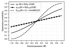
(a) SNR=-4dB

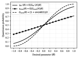
(b) SNR=0dB

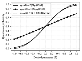
(c) SNR=4dB

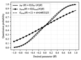
(d) SNR=8dB

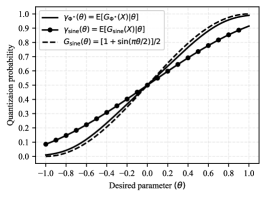
(e) SNR=12dB

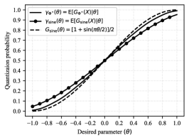
(f) SNR=16dB

Figure 12: Noisy quantization probability of the proposed and SQMLF methods under different SNRs.

In this section, we investigate the noise suppression ability and robustness of the proposed method to the observation noise, considering both the stable noisy scenario with SNR being constant during the training and test process, and the unstable scenario with fluctuating SNRs. Fig. 12 plots the noisy quantization probability of the proposed method, i.e., $\gamma_{\Phi^{*}}(\theta)=\mathbb{E}_{X}[G_{\Phi^{*}}(X)|\theta]$ defined in (8), under the stable noisy scenario. Similar to the noiseless scenario, the optimal $\gamma_{\Phi^{*}}(\theta)$ should equal to $G_{\text{sine}}(\theta)$ [26]. In particular, if $G_{\text{sine}}(X)$ is directly used as the probability controller at the sensor, its corresponding noisy quantization probability becomes $\gamma_{\text{sine}}(\theta)=\mathbb{E}_{X}[G_{\text{sine}}(X)|\theta]$ and is no longer optimal for the noisy scenario. It is observed in Fig. 12 that under differnt SNRs, $\gamma_{\Phi^{*}}(\theta)$ is closer to the optimal $G_{\text{sine}}(\theta)$ than $\gamma_{\text{sine}}(\theta)$. Besides, $\gamma_{\Phi^{*}}(\theta)$ is almost identical to $G_{\text{sine}}(\theta)$ when $\text{SNR}\geq 4\text{dB}$, whereas $\gamma_{\text{sine}}$ becomes almost identical to $G_{\text{sine}}(\theta)$ until SNR reaches 16 dB. This validates the superiority of the proposed method on the observation noise suppression.

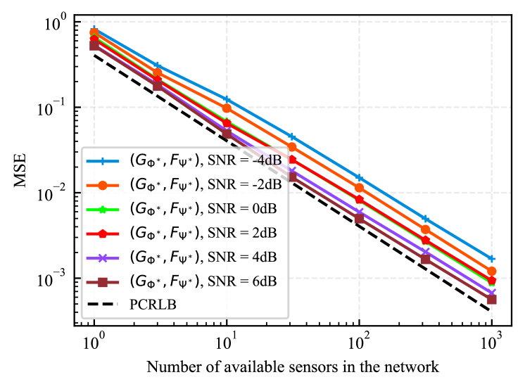
(a) Proposed method

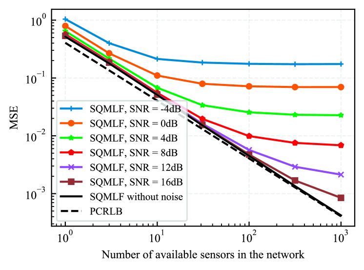
(b) SQMLF method

Figure 13: Estimation MSE of the proposed and SQMLF methods under the stable observation scenario.

Fig. 13(a) and Fig. 13(b) plot the estimation MSE of the proposed and SQMLF methods as a function of the number of sensors under the stable observation scenario. It is observed that although the SQMLF method performs nearly optimally in the ideal noiseless scenario, its performance suffers severe degradation in the noisy scenario and its estimation MSE decreases more slowly with the increasing of the number of sensors. According to Fig. 12, this observation can be attributed to the fact that the deviation of the noisy quantization probability of the SQMLF method from the optimal structure becomes more pronounced as the SNR decreases, consequently resulting in a greater performance degradation. In contrast, the estimation MSE of the proposed method under different SNRs remains close to the PCRLB and is linearly decreasing with respect to the number of sensors.

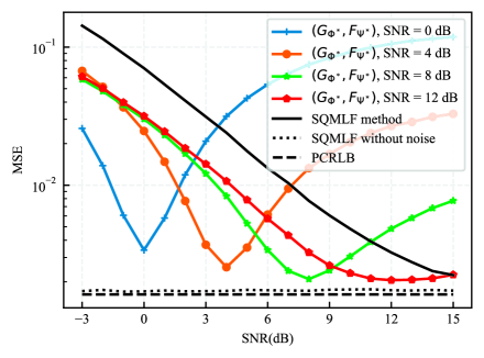
Figure 14: Estimation MSE of the proposed method under unstable observation scenario.

Next, we evaluate the robustness of the proposed method in the presence of the unstable noisy observations with fluctuating SNRs. Fig. 14 plots the estimation MSE as a function of the SNRs, with the number of sensors being set as 250. The estimation MSE of the proposed method trained under different SNRs are tested and compared with the SQMLF method. It is observed that with the increasing of the gap between the SNRs in test and training, the estimation MSE of the proposed method increases and presents to be a U-shape curve with respect to the SNRs. Consequently, in scenarios with very high SNRs, the performance of the proposed method trained under low SNRs is inferior to that of the SQMLF method. However, it is also observed that the proposed method trained under a higher SNR exhibits better robustness to the varying SNRs in test. For instance, the proposed method trained under SNR = 12 dB outperforms the SQMLF method for all SNRs tested.

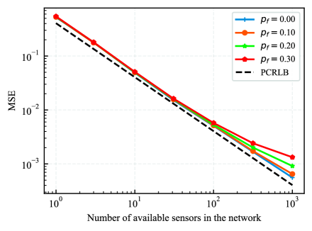
Figure 15: Robustness to a sudden spike in sensor noise,
with 4 times power spike being considered.

In practical systems, it is reasonable to account for the possibility of a sudden spike in sensor noise. We consider the scenario that all sensors in the network randomly have a 4 times power spike in its observation noise, i.e., 6 dB SNR degradation at the sensors, with the probability denoted as $p_{s}$. Fig. 15 plots the estimation MSE of our method under different values of $p_{s}$. It is observed that the estimation MSE of our proposed method remains close to the PCRLB under differnt number of sensors and values of $p_{s}$. Notably, there is only a slight increase in the MSE when the network has a huge number of sensors and a high sensor spike probability like $P_{s}=0.3$. This result provides empirical evidence that our proposed method is robust against the sudden spike in sensor noise.

V-C Multi-bit quantization

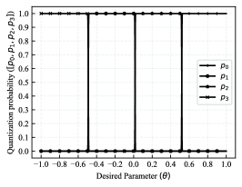
(a) $K_{s}=1$

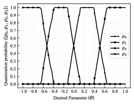
(b) $K_{s}=2$

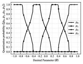
(c) $K_{s}=5$

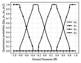
(d) $K_{s}=10$

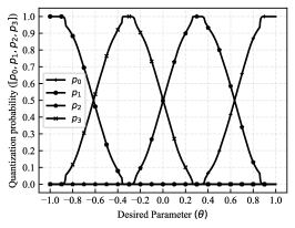
(e) $K_{s}=25$

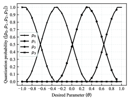
(f) $K_{s}=50$

Figure 16: 2-bit one-hot probability controller $G_{\Phi}$ trained with different $K_{S}$.

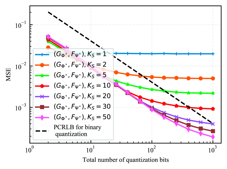
Figure 17: Estimation MSE of the 2-bit one-hot quantization vs. the total number of quantization bits, with $K_{F}=50$.

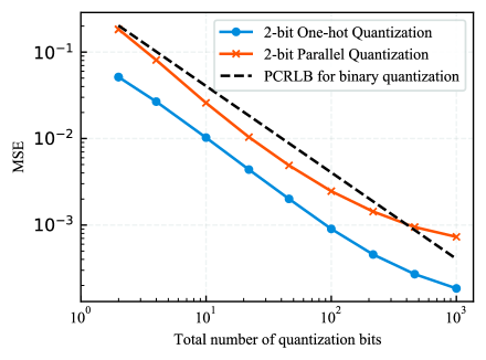
Figure 18: Estimation MSE of 2-bit one-hot quantization and 2-bit parallel quantization models, with $K_{S}=K_{F}=50$.

Finally, we investigate the performance of the proposed multi-bit parallel quantization and one-hot quantization schemes, and we select the multi-bit quantization dimension $M=2$ for both the two models. Fig. 16 plots the 2-bit one-hot probability controller $G_{\Phi^{*}}$ trained with different $K_{S}$ under the noiseless scenario. It is observed that as $K_{S}$ increases, the trained $G_{\Phi^{*}}$ converges to a stable structure with a stable quantization probability distribution on the desired parameter $\theta$. Fig. 17 plots the estimation MSE of the 2-bit one-hot quantization scheme as a function of the total number of quantization bits from all sensors. It is observed that with the increasing of $K_{S}$, the performance of the 2-bit one-hot quantization becomes asymptotically convergent and optimal, outperforming the performance limit of any binary-quantization-based estimation scheme. The result verifies the asymptotic optimality of the proposed method.

Fig. 18 plots the estimation MSE of both the 2-bit one-hot quantization and 2-bit parallel quantization schemes as a function of the total number of quantization bits from all sensors. The PCRLB of the binary quantization with respect to the number of quantization bits is plotted as a comparison. It is observed that the estimation performance of both the one-hot quantization and parallel quantitation schemes outperform the performance limit of any binary quantization scheme. Besides, it is observed that the one-hot quantization scheme exhibits better performance than the parallel one. This can be explained by the inclusion relationship between the two schemes: the set of any potential quantization probability distributions based on the parallel quantizer is a subset of those realizable by the one-hot quantizer. Therefore, the performance ceiling of the one-hot quantization scheme is at least equivalent to or better than that of the parallel scheme.

VI Conclusion

In this paper, we propose a joint model and data driven method for the quantization-based distributed estimation problem. First, for sensors with binary quantization and conditionally i.i.d. observations, the MSE lower bound for the distributed estimation is derived, and a binary probabilistic quantizer is designed to minimize this lower bound. The optimality of the mean-fusion operation at the FC for the estimation with MMSE criterion is proved and a corresponding FC design is proposed. Considering the practical scenarios that the distributions of both the desired parameter and observation noise are unknown or only the noise distribution is known, a joint model and data driven method is proposed to train the probability controller in quantizer and the estimator in FC as DNNs. By relaxing the binary quantization constraint at the sensors, the results are extended to the cases of multi-bit parallel quantization and one-hot quantization. Simulation results reveal that the proposed method outperforms state-of-the-art schemes under certain conditions.

Appendix A Proof of Proposition III.1

$$\mathbb{E}[|\theta-\hat{\theta}(\mathbf{u})|^{2}]\geq\mathbb{E}_{\theta}[\theta^{2}]-\sum_{k=0}^{K}\sum_{\mathbf{u}\in\mathcal{U}_{K}}\frac{\mathbb{E}_{\theta}^{2}\left[\theta p\left(\mathbf{u}\left|\theta\right.\right)\right]}{\mathbb{E}_{\theta}\left[p\left(\mathbf{u}\left|\theta\right.\right)\right]}=\mathbb{E}_{\theta}[\theta^{2}]-\sum_{k=0}^{K}C_{K}^{k}\frac{\mathbb{E}_{\theta}^{2}\left[\theta(\gamma(\theta))^{k}(1-\gamma(\theta))^{K-k}\right]}{\mathbb{E}_{\theta}\left[(\gamma(\theta))^{k}(1-\gamma(\theta))^{K-k}\right]}.$$ (47)

$$I_{2}(\theta)=\mathbb{E}_{\bar{u}}\left[-\frac{\partial^{2}\ln p(\bar{u}\mid\theta)}{\partial\theta^{2}}\right]=(\gamma^{\prime}(\theta))^{2}\sum_{i=0}^{K}C_{K}^{i}(\gamma(\theta))^{i-2}(1-\gamma(\theta))^{K-i-2}\left[i(1-\gamma(\theta))-(K-i)\gamma(\theta)\right]^{2}=I_{1}(\theta).$$ (50)

$$\mathbb{E}[|\theta-\hat{\theta}(\bar{u})|^{2}]\geq\mathbb{E}_{\theta,\bar{u}}[|\theta-\hat{\theta}_{\text{MMSE}}(\bar{u})|^{2}]=\mathbb{E}_{\theta}[\theta^{2}]-\sum_{k=0}^{K}C_{K}^{k}\frac{\mathbb{E}_{\theta}^{2}\left[\theta(\gamma(\theta))^{k}(1-\gamma(\theta))^{K-k}\right]}{\mathbb{E}_{\theta}\left[(\gamma(\theta))^{k}(1-\gamma(\theta))^{K-k}\right]}.$$ (51)

The FC utilizes the quantized data $\mathbf{u}=[u_{1}\cdots,u_{K}]^{T}$ from all sensors to estimate the desired parameter $\theta$ as $\hat{\theta}(\mathbf{u})$, and the estimator $\hat{\theta}(\cdot)$ determines the estimation MSE for $\theta$. According to [21], the MMSE estimator for the estimation of $\theta$ with given $\mathbf{u}$ is derived as

$$\hat{\theta}_{\text{MMSE}}\left({\mathbf{u}}\right)=\mathbb{E}_{\theta,\mathbf{u}}\left[\theta\left|\mathbf{u}\right.\right]=\frac{\mathbb{E}_{\theta}\left[\theta p\left(\mathbf{u}\left|\theta\right.\right)\right]}{\mathbb{E}_{\theta}\left[p\left(\mathbf{u}\left|\theta\right.\right)\right]},$$ (44)

and the achievable MSE in estimating $\theta$ using $\mathbf{u}$ is lower bounded by

$$\mathbb{E}[|\theta-\hat{\theta}(\mathbf{u})|^{2}]\geq \ \mathbb{E}_{\theta,\mathbf{u}}[|\theta-\hat{\theta}_{\text{MMSE}}(\mathbf{u})|^{2}]$$ (45)

$$= \ \mathbb{E}_{\theta}[\theta^{2}]-\sum_{\mathbf{u}\in\mathcal{U}}\frac{\mathbb{E}_{\theta}^{2}\left[\theta p\left(\mathbf{u}\left|\theta\right.\right)\right]}{\mathbb{E}_{\theta}\left[p\left(\mathbf{u}\left|\theta\right.\right)\right]},$$

where $\mathcal{U}=\{0,1\}^{K}$ is the set of all possible results for $\mathbf{u}$.

When the quantized data from all sensors are conditionally i.i.d. with given $\theta$, the above results can be further simplified. Define $\{\mathcal{U}_{k}\}_{k=0}^{K}$ as the sequence of non-overlapping subsets of $\mathcal{U}$, with $\mathcal{U}_{k}=\{\mathbf{u}\in\mathcal{U}|\frac{1}{K}\sum_{i=1}^{K}u_{i}=k/K\}$. It’s intuitively to see that $\mathcal{U}=\cup_{k=0}^{K}\mathcal{U}_{k}$ and $|\mathcal{U}_{k}|=C_{K}^{k}$. Besides, any $\mathbf{u}$ belonging to set $\mathcal{U}_{k}$ have the identical conditional probability with given $\theta$, i.e.,

$$p(\mathbf{u}|\theta)=(\gamma(\theta))^{k}(1-\gamma(\theta))^{K-k},$$ (46)

$\forall$ $\mathbf{u}\in\mathcal{U}_{k}$, where $\gamma(\theta)=p(u=1|\theta)$ denotes the conditional probability of any quantized data being ’1’ with given $\theta$. By subsisting (46) into (45) and utilizing $|\mathcal{U}_{k}|=C_{K}^{k}$, the MSE lower bound in (45) is rewritten as (47). This completes the proof.

Appendix B Proof of Proposition III.2

According to [26], the Fisher Information of $\mathbf{u}$ with given $\theta$ is derived as

$$I_{1}(\theta) =\mathbb{E}_{\mathbf{u}}\left[-\frac{\partial^{2}\ln p(\mathbf{u}\mid\theta)}{\partial\theta^{2}}\right]$$ (48)

$$=K\frac{(\gamma^{\prime}(\theta))^{2}}{\gamma(\theta)(1-\gamma(\theta))},$$

where $\gamma(\theta)$ is defined in (8). Based on (46), the conditional probability distribution for the average $\bar{u}$ of all quantized data with given $\theta$ is computed as

$$p\left(\bar{u}=\frac{k}{K}\bigg{|}\theta\right)=\ p(\mathbf{u}\in\mathcal{U}_{k}|\theta)=\ C_{K}^{k}\left(\gamma(\theta)\right)^{k}\left(1-\gamma(\theta)\right)^{K-k},$$ (49)

for $k=0,1,\cdots,K$. Then, by using (49), the Fisher Information of $\bar{u}$ with given $\theta$ is derived as (50).

Similar to (44), the MMSE estimator for estimating $\theta$ by using $\bar{u}$ is obtained as $\hat{\theta}_{\text{MMSE}}(\bar{u})=\mathbb{E}_{\theta}\left[\theta p\left(\bar{u}\left|\theta\right.\right)\right]/\mathbb{E}_{\theta}\left[p\left(\bar{u}\left|\theta\right.\right)\right]$. The achievable MSE lower bound for the estimation of $\theta$ with $\bar{u}$ is derived as (51), and is identical to the achievable MSE lower bound for estimating $\theta$ with $\mathbf{u}$ as derived in (7). (50) and (51) complete the proof.

Appendix C Proof of Proposition IV.1

$$p\left(\bar{\mathbf{u}}=\frac{1}{K}[i_{1},\cdots,i_{M}]^{T}\bigg{|}\theta\right)=p\left(\mathbf{U}\in\mathcal{U}_{i_{1},\cdots,i_{M}}\bigg{|}\theta\right)=\prod_{m=1}^{M}C_{K}^{i_{m}}(\gamma_{\phi_{m}}(\theta))^{i_{m}}(1-\gamma_{\phi_{m}}(\theta))^{K-i_{m}},$$ (57)

$$\mathbb{E}[|\theta-\hat{\theta}(\mathbf{U})|^{2}]\geq\mathbb{E}_{\theta,\mathbf{U}}[|\theta-\hat{\theta}_{\text{MMSE}}(\mathbf{U})|^{2}]=\mathbb{E}[\theta^{2}]-\sum_{i_{1}=0}^{K}\cdots\sum_{i_{M}=0}^{K}\frac{\mathbb{E}_{\theta}^{2}\left[\theta p\left(\mathbf{U}\in\mathcal{U}_{i_{1},\cdots,i_{M}}\bigg{|}\theta\right)\right]}{\mathbb{E}_{\theta}\left[p\left(\mathbf{U}\in\mathcal{U}_{i_{1},\cdots,i_{M}}\bigg{|}\theta\right)\right]},$$ (58)

$$\mathbb{E}[|\theta-\hat{\theta}(\bar{\mathbf{u}})|^{2}]\geq\mathbb{E}_{\theta,\bar{\mathbf{u}}}[|\theta-\hat{\theta}_{\text{MMSE}}(\bar{\mathbf{u}})|^{2}]=\mathbb{E}[\theta^{2}]-\sum_{i_{1}=0}^{K}\cdots\sum_{i_{M}=0}^{K}\frac{\mathbb{E}_{\theta}^{2}\left[\theta p\left(\bar{\mathbf{u}}=\frac{1}{K}[i_{1},\cdots,i_{M}]^{T}\left|\theta\right.\right)\right]}{\mathbb{E}_{\theta}\left[p\left(\bar{\mathbf{u}}=\frac{1}{K}[i_{1},\cdots,i_{M}]^{T}\left|\theta\right.\right)\right]},$$ (59)

$$\mathbb{E}[|\theta-\hat{\theta}(\mathbf{U})|^{2}]\geq\mathbb{E}_{\theta,\mathbf{V}}[|\theta-\hat{\theta}_{\text{MMSE}}(\mathbf{V})|^{2}]=\mathbb{E}[\theta^{2}]-\sum_{i_{1}=0}^{K}\cdots\sum_{i_{k}=0}^{L-i_{1}-\cdots-i_{k-1}}\cdots\sum_{i_{L-1}=0}^{K-i_{0}-\cdots-i_{L-2}}\frac{\mathbb{E}^{2}\left[\theta p\left(\mathbf{V}\in\mathcal{V}_{i_{0},\cdots,i_{L-1}}\bigg{|}\theta\right)\right]}{\mathbb{E}\left[p\left(\mathbf{V}\in\mathcal{V}_{i_{0},\cdots,i_{L-1}}\bigg{|}\theta\right)\right]},$$ (63)

$$\mathbb{E}[|\theta-\hat{\theta}(\bar{\mathbf{v}})|^{2}]\geq\mathbb{E}_{\theta,\bar{\mathbf{v}}}[|\theta-\hat{\theta}_{\text{MMSE}}(\bar{\mathbf{v}})|^{2}]=\mathbb{E}[\theta^{2}]-\sum_{i_{0}=0}^{K}\cdots\sum_{i_{k}=0}^{L-i_{1}-\cdots-i_{k-1}}\cdots\sum_{i_{L-1}=0}^{K-i_{1}-\cdots-i_{L-2}}\frac{\mathbb{E}_{\theta}^{2}\left[\theta p\left(\bar{\mathbf{v}}=\frac{1}{K}[i_{0},\cdots,i_{L-1}]^{T}\bigg{|}\theta\right)\right]}{\mathbb{E}_{\theta}\left[p\left(\bar{\mathbf{v}}=\frac{1}{K}[i_{0},\cdots,i_{L-1}]^{T}\bigg{|}\theta\right)\right]},$$ (64)

According to Proposition II.1, when all sensors adopt the identical $M$-bit parallel quantizer with design parameter $\Phi$, the quantized data vectors $\mathbf{u}_{1},\mathbf{u}_{2},\cdots,\mathbf{u}_{K}\in\{0,1\}^{M}$ from all $K$ sensors are conditionally i.i.d., i.e.,

$$p(\mathbf{u}_{i}=\mathbf{u}|\theta) =p(\mathbf{u}_{j}=\mathbf{u}|\theta),$$ (52)

$$p(\mathbf{u}_{1},\cdots,\mathbf{u}_{K}|\theta) =\prod_{k=1}^{K}p(\mathbf{u}_{k}|\theta),$$ (53)

$\forall i,j\in\{1,\cdots,K\},\forall\mathbf{u}\in\{0,1\}^{M}$. Then, it can be inferred from the parallel quantizer configuration in Fig. 6 that all entries of a quantized vector are conditionally independent with given $\theta$, i.e.,

$$p(\mathbf{u}_{k}|\theta)= \prod_{m=1}^{M}p([\mathbf{u}_{k}]_{m}|\theta),$$ (54)

for $k=1,2,\cdots,K$. Based on (52), (53) and (54), it can be concluded that all entries in the quantized data matrix $\mathbf{U}=[\mathbf{u}_{1}^{T},\cdots,\mathbf{u}_{K}^{T}]^{T}$ are conditionally independent with given $\theta$, i.e.,

$$p(\mathbf{U}|\theta)=\prod_{k=1}^{K}p(\mathbf{u}_{k}|\theta)=\prod_{k=1}^{K}\prod_{m=1}^{M}p([\mathbf{u}_{k}]_{m}|\theta).$$ (55)

Define $\mathcal{U}=\{0,1\}^{K\times M}$ as the set of all possible results for $\mathbf{U}$, along with a sequence of its non-overlapping subsets as $\mathcal{U}_{i_{1},\cdots,i_{M}}=\{\mathbf{U}\in\mathcal{U}|\frac{1}{K}\sum_{i=1}^{K}[\mathbf{U}]_{i,m}=\frac{1}{K}\sum_{i=1}^{K}[\mathbf{u}_{i}]_{m}=\frac{i_{m}}{K}\ \text{for}\ m=1,\cdots,M\}$ for $i_{1},\cdots,i_{M}\in\{0,\cdots,K\}$. It’s intuitively to see that $\mathcal{U}=\cup_{i_{1}=0}^{K}\cdots\cup_{i_{M}=0}^{K}\mathcal{U}_{i_{1},\cdots,i_{M}}$ and $|\mathcal{U}_{i_{1},\cdots,i_{M}}|=\prod_{m=1}^{M}C_{K}^{i_{m}}$. From (55), we have that if $\mathbf{U}\in\mathcal{U}_{i_{1},\cdots,i_{M}}$, then

$$p(\mathbf{U}|\theta)= \prod_{m=1}^{M}p\left(\frac{1}{K}\sum\nolimits_{i=1}^{K}[\mathbf{u}_{i}]_{m}=\frac{i_{m}}{K}\bigg{|}\theta\right)$$ (56)

$$= \prod_{m=1}^{M}(\gamma_{\phi_{m}}(\theta))^{i_{m}}(1-\gamma_{\phi_{m}}(\theta))^{K-i_{m}},$$

where

$$\gamma_{\phi_{m}}(\theta)=p_{\phi_{m}}([\mathbf{u}_{k}]_{m}=1|\theta),k=1,\cdots,K.$$

Define $\bar{\mathbf{u}}=\frac{1}{K}\sum_{k=1}^{K}\mathbf{u}_{k}\in\{0,1/K,\cdots,1\}^{M}$ as the mean vector of the quantized data matrix. Based on (55) and (56), the conditional probability distribution of $\bar{\mathbf{u}}$ with given $\theta$ is derived as (57), $\forall\ i_{1},\cdots,i_{M}\in\{0,1,\cdots,K\}$. By utilizing (56) and $|\mathcal{U}_{i_{1},\cdots,i_{m}}|=\prod_{m=1}^{M}C_{K}^{i_{M}}$, the achievable MSE lower bound for estimating $\theta$ using $\mathbf{U}$ is derived as (58), where $\hat{\theta}_{\text{MMSE}}(\mathbf{U})=\mathbb{E}_{\theta}\left[\theta p\left(\mathbf{U}\left|\theta\right.\right)\right]/\mathbb{E}_{\theta}\left[p\left(\mathbf{U}\left|\theta\right.\right)\right]$ is the MMSE estimator for the estimation of $\theta$ with $\mathbf{U}$. From (57), the achievable MSE lower bound for estimating $\theta$ with $\bar{\mathbf{u}}$ is derived as (59), where $\hat{\theta}_{\text{MMSE}}(\bar{\mathbf{u}})=\mathbb{E}_{\theta}\left[\theta p\left(\bar{\mathbf{u}}\left|\theta\right.\right)\right]/\mathbb{E}_{\theta}\left[p\left(\bar{\mathbf{u}}\left|\theta\right.\right)\right]$ is the corresponding MMSE estimator. By subsisting (57) into (58) and (59), we complete the proof..

Appendix D Proof of Proposition IV.2

Since the one-hot representation of a binary information is invertible, estimating the desired parameter $\theta$ with either the original quantized matrix $\mathbf{U}$ or its one-hot representation $\mathbf{V}$ achieves the identical estimation MSE, i.e.,

$$\mathrm{E}[|\theta-\hat{\theta}(\mathbf{U})|^{2}]=\mathrm{E}[|\theta-\hat{\theta}(\mathbf{V})|^{2}].$$ (60)

Similar to the analysis in (52) and (53), the quantized vectors $\mathbf{u}_{1},\cdots,\mathbf{u}_{K}$ are conditionally i.i.d. with given $\theta$, and so as their one-hot representation $\mathbf{v}_{1},\cdots,\mathbf{v}_{K}$. Define

$$\mathcal{V}=\left\{\mathbf{V}\in\{0,1\}^{K\times L}\left|\sum_{l=0}^{L-1}[\mathbf{V}]_{k,l}=1,\forall\ k\in[K]\right.\right\}$$

as the set of all possible results for $\mathbf{V}$, with $L=2^{M}$. Define a sequence of non-overlapping subsets of $\mathcal{V}$ as

$$\mathcal{V}_{i_{0},\cdots,i_{L-1}}=\left\{\mathbf{V}\in\mathcal{V}\left|\sum_{k=1}^{K}[\mathbf{V}]_{k,l}=i_{l}\ \text{for}\ l=0,\cdots,L-1\right.\right\},$$

for all positive integers $i_{0},\cdots,i_{L-1}$ satisfying $\sum_{l=0}^{L-1}i_{l}=K$. It’s intuitively to see that $\mathcal{V}=\cup_{i_{0},\cdots,i_{L-1}}\mathcal{V}_{i_{0},\cdots,i_{L-1}}$ and $|\mathcal{V}_{i_{0},\cdots,i_{L-1}}|=\prod\nolimits_{l=0}^{L-1}C_{K-i_{0}-\cdots-i_{l-1}}^{i_{l}}.$

The conditional probability distribution of $\mathbf{V}$ with given $\theta$ is derived as

$$p(\mathbf{V}|\theta)=\prod\nolimits_{l=0}^{L-1}(\gamma_{\Phi,l}(\theta))^{i_{l}},$$ (61)

$\forall\mathbf{V}\in\mathcal{V}_{i_{0},\cdots,i_{L-1}}$., where $\gamma_{\Phi,l}(\theta)=\mathbb{E}_{X}[[G_{\Phi}(X)]_{l}|\theta].$ Define $\bar{\mathbf{v}}=\frac{1}{K}\sum_{k=1}^{K}\mathbf{v}_{k}$ as the mean-one-hot-vector of $\mathbf{U}$. Based on (61), the conditional probability distribution of $\bar{\mathbf{v}}$ with given $\theta$ is derived as

$$p\left(\bar{\mathbf{v}}=\frac{1}{K}[i_{0},\cdots,i_{L-1}]^{T}\bigg{|}\theta\right)= p\left(\mathbf{V}\in\mathcal{V}_{i_{0},\cdots,i_{L-1}}\bigg{|}\theta\right)$$ (62)

$$= \prod_{l=0}^{L-1}C_{K-i_{0}-\cdots-i_{l-1}}^{i_{l}}(\gamma_{\Phi,l}(\theta))^{i_{l}},$$

for all positive integers $i_{0},\cdots,i_{L-1}$ satisfying $\sum_{l=0}^{L-1}i_{l}=K$.

By utilizing (60) and (61), the achievable MSE lower bound for estimating $\theta$ with $\mathbf{U}$ is derived as (63), where $\hat{\theta}_{\text{MMSE}}(\mathbf{V})=\mathbb{E}_{\theta}\left[\theta p\left(\mathbf{V}\left|\theta\right.\right)\right]/\mathbb{E}_{\theta}\left[p\left(\mathbf{V}\left|\theta\right.\right)\right]$ is the MMSE estimator for estimating $\theta$ using $\mathbf{V}$. The achievable MSE lower bound for estimating $\theta$ using $\bar{\mathbf{v}}$ is derived as (64), where $\hat{\theta}_{\text{MMSE}}(\bar{\mathbf{v}})=\mathbb{E}_{\theta}\left[\theta p\left(\bar{\mathbf{v}}\left|\theta\right.\right)\right]/\mathbb{E}_{\theta}\left[p\left(\bar{\mathbf{v}}\left|\theta\right.\right)\right]$ is the corresponding MMSE estimator. By subsisting (62) into (63) and (64), we complete the proof.

Meng He (Member, IEEE) received the B.E. degree in communication engineering from University of Electronic Science and Technology of China, Chengdu, China, in 2017, and the Ph.D. degree in computer and information engineering from The Chinese University of Hong Kong, Shenzhen, China, in 2023. He was a TPC member for IEEE GLOBECOM 2019-2022. He has been serving as a reviewer for IEEE TRANSACTIONS ON WIRELESS COMMUNICATIONS, and Journal of Communications and Information Networks. His current research interests include full-duplex communications, distributed estimation in wireless sensor networks and deep learning.

Ran Li (Member, IEEE) received the B.E. degree in communication engineering from University of Electronic Science and Technology of China, Chengdu, China, in 2017, and the Ph.D. degree in computer and information engineering from The Chinese University of Hong Kong, Shenzhen, China, in 2023. His current research interests include reinforcement learning and resource allocation in wireless networks.

Chuan Huang (S’09–M’13) received his Ph.D. in Electrical Engineering from Texas A&M University, College Station, Texas, USA, in 2012. From August 2012 to July 2014, he was a Research Associate with Princeton University, Princeton, NJ, USA, and then a Research Assistant Professor with Arizona State University, Tempe, AZ, USA. He is currently an Associate Professor with The Chinese University of Hong Kong, Shenzhen. His current research interests include wireless communications and signal processing. He has been serving as an Editor for IEEE TRANSACTIONS ON WIRELESS COMMUNICATIONS, IEEE ACCESS, Journal of Communications and Information Networks, and IEEE WIRELESS COMMUNICATIONS LETTERS. He served as the Symposium Chair for IEEE GLOBECOM 2019 and IEEE ICCC 2019 and 2020.

Shulong Zhang received the B.E. degree in Control Science and Engineering from Harbin Institute of Technology, Harbin, China, in 2015, and the Master’s degree in Control Science and Engineering from National University of Defense Science and Technology, Changsha, China. He is currently working at SF Technology Co., Ltd. as a system simulation engineer. His current research interests include digital twin and network planning.

References

- [1] M. He, C. Huang, and S. Jiang, “On probabilistic quantization and mean-value fusion design for distributed estimation in sensor networks,” in 2022 IEEE/CIC International Conference on Communications in China (ICCC), 2022, pp. 1107–1112.
- [2] A. Kottas, Z. Wang, and A. Rodríguez, “Spatial modeling for risk assessment of extreme values from environmental time series: A bayesian nonparametric approach,” Environmetrics, vol. 23, no. 8, pp. 649–662, Dec. 2012.
- [3] J. P. French and S. R. Sain, “Spatio-temporal exceedance locations and confidence regions,” Ann. Appl. Stat., vol. 7, no. 3, pp. 1421–1449, Sep. 2013.
- [4] F. S. Cattivelli and A. H. Sayed, “Diffusion LMS strategies for distributed estimation,” IEEE Trans. Signal Process., vol. 58, no. 3, pp. 1035–1048, Mar. 2010.
- [5] I. D. Schizas, A. Ribeiro, and G. B. Giannakis, “Consensus in Ad Hoc WSNs with noisy links-part I: Distributed estimation of deterministic signals,” IEEE Trans. Signal Process., vol. 56, no. 1, pp. 350–364, Jan. 2008.
- [6] F. S. Cattivelli, C. G. Lopes, and A. H. Sayed, “Diffusion recursive least-squares for distributed estimation over adaptive networks,” IEEE Trans. Signal Process., vol. 56, no. 5, pp. 1865–1877, May 2008.
- [7] A. Ribeiro and G. Giannakis, “Bandwidth-constrained distributed estimation for wireless sensor networks-part I: Gaussian case,” IEEE Trans. Signal Process., vol. 54, no. 3, pp. 1131–1143, Mar. 2006.
- [8] P. Venkitasubramaniam, G. Mergen, L. Tong, and A. Swami, “Quantization for distributed estimation in large scale sensor networks,” in 2005 3rd International Conference on Intelligent Sensing and Information Processing, Dec. 2005, pp. 121–127.
- [9] T. Wu and Q. Cheng, “One-bit quantizer design for distributed estimation under the minimax criterion,” in 2010 IEEE 71st Vehicular Technology Conference, May 2010, pp. 1–5.
- [10] A. Sani and A. Vosoughi, “Distributed vector estimation for power- and bandwidth-constrained wireless sensor networks,” IEEE Trans. Signal Process., vol. 64, no. 15, pp. 3879–3894, Aug. 2016.
- [11] J.-J. Xiao, A. Ribeiro, Z.-Q. Luo, and G. Giannakis, “Distributed compression-estimation using wireless sensor networks,” IEEE Signal Process. Mag., Special Issue on Distributed Signal Processing for Sensor Networks, vol. 23, no. 4, pp. 27–41, Jul. 2006.
- [12] J. Zhu, X. Lin, R. S. Blum, and Y. Gu, “Parameter estimation from quantized observations in multiplicative noise environments,” IEEE Trans. Signal Process., vol. 63, no. 15, pp. 4037–4050, Aug. 2015.
- [13] M. El Gamal and L. Lai, “On rate requirements for achieving the centralized performance in distributed estimation,” IEEE Trans. Signal Process., vol. 65, no. 8, pp. 2020–2032, Apr. 2017.
- [14] W.-M. Lam and A. Reibman, “Design of quantizers for decentralized estimation systems,” IEEE Trans. Commun., vol. 41, no. 11, pp. 1602–1605, Nov. 1993.
- [15] J. Gubner, “Distributed estimation and quantization,” IEEE Trans. Inf. Theory, vol. 39, no. 4, pp. 1456–1459, Jul. 1993.
- [16] A. Ribeiro and G. Giannakis, “Bandwidth-constrained distributed estimation for wireless sensor networks-part II: unknown probability density function,” IEEE Trans. Signal Process., vol. 54, no. 7, pp. 2784–2796, Jul. 2006.
- [17] Z.-Q. Luo, “Universal decentralized estimation in a bandwidth constrained sensor network,” IEEE Trans. Inf. Theory, vol. 51, no. 6, pp. 2210–2219, June 2005.
- [18] J. Li and G. AlRegib, “Rate-constrained distributed estimation in wireless sensor networks,” IEEE Trans. Signal Process., vol. 55, no. 5, pp. 1634–1643, May 2007.
- [19] S. Ghazanfari-Rad and F. Labeau, “Formulation and analysis of lms adaptive networks for distributed estimation in the presence of transmission errors,” IEEE Internet of Things Journal, vol. 3, no. 2, pp. 146–160, 2015.
- [20] H. Poor, “Fine quantization in signal detection and estimation,” IEEE Trans. Inf. Theory, vol. 34, no. 5, pp. 960–972, Sep. 1988.
- [21] T. A. Schonhoff and A. A. Giordano, Detection and estimation theory and its applications. Prentice Hall, 2006.
- [22] S. Lloyd, “Least squares quantization in pcm,” IEEE Trans. Inf. Theory, vol. 28, no. 2, pp. 129–137, Mar. 1982.
- [23] J. Max, “Quantizing for minimum distortion,” IEEE Trans. Inf. Theory, vol. 6, no. 1, pp. 7–12, Mar. 1960.
- [24] M. Shirazi and A. Vosoughi, “Bayesian cramér-rao bound for distributed estimation of correlated data with non-linear observation model,” in 2014 48th Asilomar Conference on Signals, Systems and Computers, Nov. 2014, pp. 1484–1488.
- [25] A. Sani and A. Vosoughi, “On distributed linear estimation with observation model uncertainties,” IEEE Trans. Signal Process., vol. 66, no. 12, pp. 3212–3227, June 2018.
- [26] H. Chen and P. K. Varshney, “Performance limit for distributed estimation systems with identical one-bit quantizers,” IEEE Trans. Signal Process., vol. 58, no. 1, pp. 466–471, Jan. 2010.
- [27] S. Kar, H. Chen, and P. K. Varshney, “Optimal identical binary quantizer design for distributed estimation,” IEEE Trans. Signal Process., vol. 60, no. 7, pp. 3896–3901, Jul. 2012.
- [28] A. Vempaty, H. He, B. Chen, and P. K. Varshney, “On quantizer design for distributed bayesian estimation in sensor networks,” IEEE Trans. Signal Process., vol. 62, no. 20, pp. 5359–5369, Oct. 2014.
- [29] X. Li, J. Guo, U. Rogers, and H. Chen, “Asymptotic optimal quantizer design for distributed bayesian estimation,” in 2016 IEEE International Conference on Acoustics, Speech and Signal Processing (ICASSP), Mar. 2016, pp. 3711–3715.
- [30] R. M. Gray and T. G. Stockham, “Dithered quantizers,” IEEE Trans. Inf. Theory, vol. 39, no. 3, pp. 805–812, May 1993.
- [31] T. Oshea and J. Hoydis, “An introduction to deep learning for the physical layer,” IEEE Trans. Cogn. Commun. Netw., vol. 3, no. 4, pp. 563–575, Dec. 2017.
- [32] K. He, X. Zhang, S. Ren, and J. Sun, “Delving deep into rectifiers: Surpassing human-level performance on imagenet classification,” in Proceedings of the IEEE international conference on computer vision, 2015, pp. 1026–1034.