Resummation and renormalization of kinematical effects in inclusive $P$-wave quarkonium production

Abstract

We investigate the renormalization properties of the shape function formalism for inclusive production of $P$-wave heavy quarkonia, which arises from resumming a class of corrections coming from kinematical effects associated with the motion of the heavy quark and antiquark pair relative to the quarkonium. Such kinematical effects are encoded in the nonperturbative shape functions, which are normalized to the corresponding nonrelativistic QCD long-distance matrix elements. By using the known ultraviolet divergences in the matrix elements, we derive the large-momentum asymptotic behavior of the shape functions. This strongly constrains the form of the shape functions and significantly reduces the dependence on the nonperturbative model. Based on these results we show that the shape function formalism at loop level can be useful in taming the threshold logarithms at large transverse momentum, and at small transverse momentum the kinematical corrections reduce the sizes of $\chi_{c}$ and $\chi_{b}$ cross sections which may improve agreement with measurements.

1 Introduction

First-principles based studies of inclusive heavy quarkonium production phenomenology have usually been done in the nonrelativistic QCD (NRQCD) factorization formalism Bodwin:1994jh . In this formalism, the production rate of a heavy quarkonium is factorized into products of perturbatively calculable short-distance coefficients and nonperturbative long-distance matrix elements. The predictive power of the factorization formalism comes from the universality and the nonrelativistic power counting of the matrix elements, which allow quantitative descriptions of production rates once values of a few nonperturbative parameters are determined from experiments. This approach had limited success in deciphering the heavy quarkonium production mechanism: as have been discussed in the literature, results from the global fit analyses of $J/\psi$ production based mostly on total inclusive production and low transverse momentum data Butenschoen:2010rq ; Butenschoen:2011yh ; Butenschoen:2011ks ; Butenschoen:2012qh ; Butenschoen:2012qr ; Butenschoen:2012px are in conflict with analyses mostly based on large transverse momentum data Ma:2010yw ; Gong:2012ug ; Han:2014kxa ; Bodwin:2015iua ; Feng:2018ukp ; Chung:2018lyq ; Brambilla:2022rjd ; Chung:2022uih ; Brambilla:2022ayc and with LHC measurements of polarized and polarization-summed hadroproduction rates at large transverse momentum. Similarly, in the case of $\psi(2S)$, NRQCD analyses generally have difficulty explaining production rates with transverse momentum smaller than 2 – 3 times the heavy quarkonium mass Han:2014kxa ; Bodwin:2015iua ; Butenschoen:2022qka ; Brambilla:2022rjd ; Brambilla:2022ayc . Moreover, some matrix element determinations can lead to large uncertainties in the cross sections at very large transverse momentum due to mixings of contributions from different channels, which comes from renormalization of the long-distance matrix elements Butenschoen:2022qka . These call for investigation of possible refinements to the NRQCD factorization approach in quarkonium production phenomenology that can modify the transverse momentum dependences of the cross sections.

In an inclusive production process, the quark $Q$ and antiquark $\bar{Q}$ produced in a hard process can have nonzero total momentum relative to the heavy quarkonium. This happens because the $Q\bar{Q}$ can emit an arbitrary number of soft particles before evolving into a heavy quarkonium, which carry small but nonzero momenta. This kinematical effect gives rise to operators that are given in the form of total derivatives of the $Q\bar{Q}$ bilinear Mannel:1994xh ; Rothstein:1997ac ; Mannel:1997uk . While these operators are suppressed by powers of the heavy-quark velocity $v$ in the nonrelativistic power counting of NRQCD, they can be enhanced due to threshold effects associated with the boundary of phase space Rothstein:1997ac ; Mannel:1997uk . The corrections from these operators can be partially resummed to all orders in $v$, which leads to the shape function formalism developed in ref. Beneke:1997qw , where products of short-distance coefficients and NRQCD matrix elements are replaced by convolutions of short-distance coefficients and nonperturbative shape functions. Here, shape functions are functions of the momentum of the $Q\bar{Q}$ pair in the rest frame of the heavy quarkonium in the final state. A similar formalism based on the soft-collinear effective theory have been developed in ref. Fleming:2003gt . It has been anticipated that the kinematical effects computed in the shape function formalism will have a significant impact on the transverse-momentum differential cross sections of heavy quarkonia. However, phenomenological applications of this formalism have been limited, because shape functions are nonperturbative functions that are in general unknown, other than the fact that they are normalized to the corresponding NRQCD matrix elements. That is, unless one can determine the shape functions from first principles, the shape function formalism has less predictive power than the NRQCD factorization formalism.

Another shortcoming of the shape function formalism is that, in its original form, it does not correctly incorporate the renormalization of the NRQCD matrix elements. Because the shape functions are normalized to the NRQCD matrix elements, their normalizations must reproduce the same ultraviolet (UV) divergences in the matrix elements for the formalism to be consistent with NRQCD. This point has not been considered in the development of the formalism in refs. Beneke:1997qw ; Fleming:2003gt , because at that time, phenomenological applications of the NRQCD factorization formalism have usually been done at leading order in the strong coupling.

The UV divergences in the normalizations of the shape functions can have important phenomenological implications. First, the known UV divergences fix the large-momentum asymptotic behaviors of the shape functions, which strongly constrain their forms. This happens because, as we will see later, the UV divergence comes from the normalization integral of the shape function over the momentum of the $Q\bar{Q}$ in the quarkonium rest frame. This significantly enhances the predictive power of the shape function formalism, compared to existing studies where models for the shape functions had to be chosen arbitrarily. Second, the UV divergences induce momentum-dependent mixings between channels, which modify the matching conditions that are needed to determine the short-distance coefficients. This makes the matching conditions originally obtained in ref. Beneke:1997qw invalid beyond tree level, because there the mixing effects were not taken into account. Since current-day phenomenological studies of quarkonium production are usually carried out at next-to-leading order (NLO) in $\alpha_{s}$, a correct derivation of the matching conditions incorporating mixing effects is necessary.

In this work, we consider the inclusive production of $P$-wave heavy quarkonia in the shape function formalism at NLO accuracy. We focus on the simpler case of production of $P$-wave quarkonia, which involves only one unknown nonperturbative matrix element, and the renormalization of the matrix elements is less complicated compared to the $S$-wave case. The $P$-wave production rate is also important in understanding the feeddown contributions in $S$-wave quarkonium production. In order to correctly incorporate the renormalization of NRQCD matrix elements, we compute the shape functions in perturbative QCD at NLO accuracy, which lets us obtain one-loop matching conditions for the shape function formalism that are necessary for computing the short-distance coefficients. This also gives us the large-momentum asymptotic forms of the shape functions, which, together with the normalization condition, help strongly constrain the nonperturbative form of the shape function and significantly reduce the model dependence. Furthermore, we can compute the shape functions in terms of quarkonium wavefunctions and universal gluonic operator vacuum expectation values using the potential NRQCD (pNRQCD) formalism developed in refs. Pineda:1997bj ; Brambilla:1999xf ; Brambilla:2001xy ; Brambilla:2002nu ; Brambilla:2004jw ; Brambilla:2020ojz ; Brambilla:2021abf ; Brambilla:2022rjd ; Brambilla:2022ayc . Although such a calculation does not yet lead to a first-principles determination of the shape functions due to our lack of knowledge of the nonperturbative dynamics of gluons, the universality of the gluon operator vacuum expectation values can enhance the predictive power of the formalism, similarly to the pNRQCD calculations of NRQCD matrix elements. Based on the results for the shape functions and the corresponding short-distance coefficients we obtain in this work, we resum the kinematical corrections to inclusive $\chi_{c}$ and $\chi_{b}$ hadroproduction rates at small and large transverse momentum.

This paper is organized as follows. In sec. 2 we introduce the NRQCD and shape function formalisms for $P$-wave quarkonium production. In sec. 3 we compute the shape functions in perturbative QCD, which are necessary in deriving loop-level matching conditions for the shape function formalism. In sec. 4 we compute the shape functions nonperturbatively in pNRQCD and obtain expressions in terms of quarkonium wavefunctions and universal gluonic operator vacuum expectation values. In sec. 5 we establish the matching conditions for the shape function formalism that allow us to obtain short-distance coefficients from the known results in NRQCD. By using these results we discuss phenomenological applications of the shape function formalism for hadroproduction of $\chi_{c}$ and $\chi_{b}$ at large and small transverse momentum in sec. 6. We conclude in sec. 7.

2 Shape function formalism for $P$-wave production

We first review the NRQCD factorization formalism for production of a $\chi_{QJ}$ for $J=0$, 1, and 2, where $Q=c$ or $b$. At leading order in $v$, the inclusive production cross section of $\chi_{QJ}$ is given by Bodwin:1994jh

$$\sigma[\chi_{QJ}(P)]=(2J+1)\left(c_{{}^{3}P_{J}^{[1]}}(P)\langle{\cal O}^{\chi_{Q0}}(^{3}P_{0}^{[1]})\rangle+c_{{}^{3}S_{1}^{[8]}}(P)\langle{\cal O}^{\chi_{Q0}}(^{3}S_{1}^{[8]})\rangle\right),$$ (1)

where $P$ is the momentum of the $\chi_{QJ}$, $c_{{}^{3}P_{J}^{[1]}}(P)$ and $c_{{}^{3}S_{1}^{[8]}}(P)$ are short-distance coefficients, $\langle{\cal O}\rangle$ denote the vacuum expectation value of an operator ${\cal O}$, and the $\langle{\cal O}^{\chi_{Q0}}(^{3}P_{0}^{[1]})\rangle$ and $\langle{\cal O}^{\chi_{Q0}}(^{3}S_{1}^{[8]})\rangle$ are NRQCD long-distance matrix elements that describe the evolution of a $Q\bar{Q}$ in a specific color and angular momentum state into $\chi_{Q0}$+anything. We have used the heavy-quark spin symmetry relations, which are valid up to corrections of order $v^{2}$, to write the $\chi_{QJ}$ matrix elements in terms of the ones for $\chi_{Q0}$. The definitions of the NRQCD matrix elements read

$$\langle{\cal O}^{\chi_{Q0}}(^{3}P_{0}^{[1]})\rangle = \frac{1}{d-1}\langle\chi^{\dagger}(-\tfrac{i}{2}\overleftrightarrow{\bm{D}}\cdot\bm{\sigma})\psi{\cal P}_{\chi_{Q0}}\psi^{\dagger}(-\tfrac{i}{2}\overleftrightarrow{\bm{D}}\cdot\bm{\sigma})\chi\rangle,$$ (2a)

$$\langle{\cal O}^{\chi_{Q0}}(^{3}S_{1}^{[8]})\rangle = \langle\chi^{\dagger}\sigma^{i}T^{a}\psi\Phi_{\ell}^{{\dagger}ab}(0){\cal P}_{\chi_{Q0}}\Phi_{\ell}^{bc}(0)\psi^{\dagger}\sigma^{i}T^{c}\chi\rangle,$$ (2b)

where $d$ is the number of spacetime dimensions, $\psi$ and $\chi$ are Pauli spinor fields that destroy and create a heavy quark and antiquark, respectively, $\bm{D}=\bm{\nabla}-ig\bm{A}$ is the gauge-covariant derivative, $\bm{A}$ is the gluon field, $\overleftrightarrow{\bm{D}}$ is defined through the relation $\psi^{\dagger}\overleftrightarrow{\bm{D}}\chi=\psi^{\dagger}\bm{D}\chi-(\bm{D}\psi)^{\dagger}\chi$, $\bm{\sigma}$ is a Pauli matrix, ${\cal P}_{\chi_{Q0}}$ is a projection onto states that include the quarkonium $\chi_{Q0}$ at rest, and $T^{a}$ is a $SU(3)$ color matrix. In the color-octet operator ${\cal O}^{\chi_{Q0}}(^{3}S_{1}^{[8]})$, the adjoint Wilson line $\Phi_{\ell}(x)=P\exp[-ig\int_{0}^{\infty}dz\ell\cdot A(x+\ell z)]$, where $P$ is the path ordering for color matrices and $\ell$ is an arbitrary lightlike direction, is inserted to ensure the gauge invariance of the matrix element Nayak:2005rw ; Nayak:2005rt ; Nayak:2006fm . The $Q\bar{Q}$ bilinears on the right and left of the projection operator ${\cal P}_{\chi_{Q0}}$ create and destroy a $Q\bar{Q}$ in a specific color and angular momentum state.

Equation (1) follows from a factorization conjecture, where the nonperturbative long-distance physics of scales below the heavy-quark mass $m$ is encoded in the matrix elements, while the short-distance coefficients depend only on the short-distance process of the perturbative production of $Q\bar{Q}$. In this case, a $Q\bar{Q}$ in either a color-singlet or color-octet state can evolve into a color-singlet quarkonium by emitting an arbitrary number of light particles with soft momentum of scales $mv$ and lower. Hence, the $Q\bar{Q}$ produced in a short-distance process can have a relative momentum of order $mv$ with respect to the produced quarkonium. The nonvanishing of this relative momentum can have a significant effect on quarkonium production observables, if the $Q\bar{Q}$ is produced in the short-distance process predominantly near the boundary of phase space. In this case, logarithmic corrections to the short-distance coefficients from radiation of soft gluons can become enhanced, which must be matched with the effect of soft gluon emission in the NRQCD matrix elements. Also, in experimental observables kinematical cuts on the energy or momentum of the quarkonium are often taken, which can be sensitive to the order-$mv$ change in the quarkonium momentum. In the NRQCD factorization formula in its usual form, the effect of the relative momentum between the $Q\bar{Q}$ and the quarkonium is not taken into account, because the scales $mv$ and lower do not affect the short-distance coefficients. Hence, in NRQCD, the momentum of the $Q\bar{Q}$ produced in the hard process is identified with the momentum of the quarkonium. Therefore, predictions based on the factorization formula in eq. (1) can suffer from large corrections from kinematical effects associated with the motion of the $Q\bar{Q}$ in the quarkonium rest frame.

The kinematical effects can be taken into account by including contributions from certain higher dimensional operators that involve total derivatives of the $Q\bar{Q}$ bilinears in the factorization formula. The motion of the $Q\bar{Q}$ along a momentum $l$ gives rise to the following forms of higher dimensional matrix elements Mannel:1994xh ; Rothstein:1997ac ; Mannel:1997uk :

$$\frac{1}{d-1}\langle\chi^{\dagger}(-\tfrac{i}{2}\overleftrightarrow{\bm{D}}\cdot\bm{\sigma})\psi{\cal P}_{\chi_{Q0}}(l\cdot D)^{n}\psi^{\dagger}(-\tfrac{i}{2}\overleftrightarrow{\bm{D}}\cdot\bm{\sigma})\chi\rangle,$$ (3a)

$$\langle\chi^{\dagger}\sigma^{i}T^{a}\psi\Phi_{\ell}^{{\dagger}ab}(0){\cal P}_{\chi_{Q0}}(l\cdot D)^{n}\Phi_{\ell}^{bc}(0)\psi^{\dagger}\sigma^{i}T^{c}\chi\rangle,$$ (3b)

where the derivatives $D$ act to the right and $n$ is a positive integer. The operators involving derivatives on the left of the projector ${\cal P}_{\chi_{Q0}}$ can be obtained by using Hermitian conjugation and the invariance of the vacuum. Note that matrix elements of this kind do not appear in exclusive production due to conservation of energy and momentum. As have been shown in refs. Beneke:1997qw ; Fleming:2003gt , near the boundary of phase space, contributions from the above matrix elements associated with a lightlike momentum $l$ collinear to the quarkonium momentum $P$ become enhanced. These matrix elements can be obtained from moments of the “shape functions” defined by

$${\cal S}^{\chi_{Q0}}_{{}^{3}P_{0}^{[1]}}(l_{+}) = \frac{1}{d-1}\langle\chi^{\dagger}(-\tfrac{i}{2}\overleftrightarrow{\bm{D}}\cdot\bm{\sigma})\psi{\cal P}_{\chi_{Q0}}\delta(l_{+}-iD_{+})\psi^{\dagger}(-\tfrac{i}{2}\overleftrightarrow{\bm{D}}\cdot\bm{\sigma})\chi\rangle,$$ (4a)

$${\cal S}^{\chi_{Q0}}_{{}^{3}S_{1}^{[8]}}(l_{+}) = \langle\chi^{\dagger}\sigma^{i}T^{a}\psi\Phi_{\ell}^{{\dagger}ab}(0){\cal P}_{\chi_{Q0}}\delta(l_{+}-iD_{+})\Phi_{\ell}^{bc}(0)\psi^{\dagger}\sigma^{i}T^{c}\chi\rangle,$$ (4b)

where $\delta(x)$ is the Dirac delta function, and the $+$ direction is defined along the quarkonium momentum $P$. We take the convention $l_{\pm}=l_{0}\pm l_{z}$, where $l_{z}=\bm{P}\cdot\bm{l}/|\bm{P}|$ in the frame where the quarkonium three-momentum $\bm{P}$ is nonzero. From the above definitions, it is evident that they are formally normalized by $\int_{0}^{\infty}dl_{+}{\cal S}^{\chi_{Q0}}_{{}^{3}P_{0}^{[1]}}(l_{+})=\langle{\cal O}^{\chi_{Q0}}(^{3}P_{0}^{[1]})\rangle$ and $\int_{0}^{\infty}dl_{+}{\cal S}^{\chi_{Q0}}_{{}^{3}S_{1}^{[8]}}(l_{+})=\langle{\cal O}^{\chi_{Q0}}(^{3}S_{1}^{[8]})\rangle$. The shape functions defined in eqs. (4) can be interpreted as the probabilities for a $Q\bar{Q}$ to evolve into a quarkonium after emitting soft particles with total momentum $l$. The requirement that NRQCD factorization holds after inclusion of the higher dimensional matrix elements in eqs. (3) constrains the shape functions to be defined only for $l_{+}>0$. This is because a negative $l_{+}$, corresponding to the case where the $Q\bar{Q}$ absorbs energy before evolving into a quarkonium, implies that the soft interactions between the $Q\bar{Q}$ and the environment are not disentangled, and factorization is explicitly broken Beneke:1999gq .

While the lightlike direction $\ell$ of the gauge-completion Wilson line is arbitrarily chosen in the definition of the color-octet matrix element, its origin is the direction of the heavy quarkonium momentum in a boosted frame such as the hadron CM frame Nayak:2005rw ; Nayak:2005rt , just like the direction of the lightlike momentum $l$. Although the gauge-completion Wilson line will not play a role in the phenomenological analysis of $\chi_{QJ}$ production at NLO accuracy, because diagrams that involve the gauge-completion Wilson line begin to appear from two loops Nayak:2005rw ; Nayak:2005rt ; Nayak:2006fm ; Bodwin:2019bpf , for definiteness we will take the direction $\ell$ to be the same as $l$.

The factorization assumption leads to the following form of the factorization formula for the shape function formalism

$$\sigma[{\chi_{QJ}(P)}] = (2J+1)\int_{0}^{\infty}dl_{+}\left[s_{{}^{3}P_{J}^{[1]}}(P+l){\cal S}_{{}^{3}P_{0}^{[1]}}^{\chi_{Q0}}(l_{+})+s_{{}^{3}S_{1}^{[8]}}(P+l){\cal S}_{{}^{3}S_{1}^{[8]}}^{\chi_{Q0}}(l_{+})\right],$$ (5)

where the $s_{N}(P+l)$ are the short-distance coefficients in the shape function formalism, which must be functions of the $Q\bar{Q}$ momentum $P+l$. This follows from the fact that the shape function formalism is obtained by resumming contributions from higher dimensional NRQCD matrix elements of the form given in eqs. (3), which implies that the coefficients $s_{N}(P+l)$ can be obtained from the standard NRQCD matching procedure by using the perturbative cross sections $\sigma[Q\bar{Q}(P+l)]$, formally by expanding in powers of $l$. In ref. Beneke:1997qw , it has thus been suggested that the short-distance coefficients in the shape function formalism are simply given by $s_{N}(P+l)=c_{N}(P+l)$. However, this can become invalid beyond tree level, because UV divergences in the NRQCD matrix elements induce mixing between the two channels, which occur in different forms in NRQCD and shape function formalisms.

Let us compare the matching conditions for the two formalisms. The matching conditions that determine the NRQCD short-distance coefficients read

$$\sigma[Q\bar{Q}(^{3}P_{J}^{[1]})(P)] = (2J\!+\!1)\Big{(}c_{{}^{3}P_{J}^{[1]}}(P)\langle{\cal O}^{Q\bar{Q}(^{3}P_{0}^{[1]})}(^{3}P_{0}^{[1]})\rangle$$ (6a)

$$\hskip 43.05542pt+c_{{}^{3}S_{1}^{[8]}}(P)\langle{\cal O}^{Q\bar{Q}(^{3}P_{0}^{[1]})}(^{3}S_{1}^{[8]})\rangle\Big{)},$$

$$\sigma[Q\bar{Q}(^{3}S_{1}^{[8]})(P)] = c_{{}^{3}S_{1}^{[8]}}(P)\langle{\cal O}^{Q\bar{Q}(^{3}S_{1}^{[8]})}(^{3}S_{1}^{[8]})\rangle,$$ (6b)

which we obtain from eq. (1) by replacing the quarkonium state by $Q\bar{Q}$ states with definite color and angular momentum. We used the fact that, as we will see later, the matrix element $\langle{\cal O}^{Q\bar{Q}(^{3}S_{1}^{[8]})}(^{3}P_{0}^{[1]})\rangle$ vanishes at current accuracy in $v$. At tree level, only the matrix elements $\langle{\cal O}^{Q\bar{Q}(^{3}P_{0}^{[1]})}(^{3}P_{0}^{[1]})\rangle$ and $\langle{\cal O}^{Q\bar{Q}(^{3}S_{1}^{[8]})}(^{3}S_{1}^{[8]})\rangle$ are nonzero, so that at this level the short-distance coefficients $c_{N}(P)$ are proportional to the $Q\bar{Q}$ cross sections $\sigma[Q\bar{Q}(N)(P)]$ for $N={}^{3}P_{J}^{[1]}$ and ${}^{3}S_{1}^{[8]}$. However, at one-loop level the color-octet matrix element $\langle{\cal O}^{Q\bar{Q}(^{3}S_{1}^{[8]})}(^{3}S_{1}^{[8]})\rangle$ acquires a logarithmic UV divergence that is proportional to the color-singlet matrix element $\langle{\cal O}^{Q\bar{Q}(^{3}P_{0}^{[1]})}(^{3}P_{0}^{[1]})\rangle$. After the UV divergence is removed through renormalization, the short-distance coefficient $c_{{}^{3}P_{J}^{[1]}}(P)$ acquires a logarithmic scale dependence that is proportional to $c_{{}^{3}S_{1}^{[8]}}(P)$, which cancels the scale dependence of the color-octet matrix element in the factorization formula. This kind of mixing occurs also in the shape function formalism, but in a different, $l$-dependent manner. The matching conditions that determine the short-distance coefficients $s_{N}(P+l)$ in the shape function formalism read

$$\sigma[Q\bar{Q}(^{3}P_{J}^{[1]})(P)] = (2J+1)\int_{0}^{\infty}dl_{+}\bigg{[}s_{{}^{3}P_{J}^{[1]}}(P+l){\cal S}_{{}^{3}P_{0}^{[1]}}^{Q\bar{Q}(^{3}P_{0}^{[1]})}(l_{+})$$ (7a)

$$\hskip 86.11084pt+s_{{}^{3}S_{1}^{[8]}}(P+l){\cal S}_{{}^{3}S_{1}^{[8]}}^{Q\bar{Q}(^{3}P_{0}^{[1]})}(l_{+})\bigg{]},$$

$$\sigma[Q\bar{Q}(^{3}S_{1}^{[8]})(P)] = \int_{0}^{\infty}dl_{+}\,s_{{}^{3}S_{1}^{[8]}}(P+l){\cal S}_{{}^{3}S_{1}^{[8]}}^{Q\bar{Q}(^{3}S_{1}^{[8]})}(l_{+}),$$ (7b)

which we obtain from eq. (5) by replacing the quarkonium state by $Q\bar{Q}$ states with definite color and angular momentum. We have used the fact that, as we will show later, the shape function ${\cal S}_{{}^{3}P_{0}^{[1]}}^{Q\bar{Q}(^{3}S_{1}^{[8]})}(l_{+})$ vanishes at current accuracy in $v$. Similarly to the matching calculation in NRQCD, determination of $s_{N}(P+l)$ at one-loop level requires computation of the shape functions ${\cal S}_{{}^{3}P_{0}^{[1]}}^{Q\bar{Q}(^{3}P_{0}^{[1]})}(l_{+})$, ${\cal S}_{{}^{3}S_{1}^{[8]}}^{Q\bar{Q}(^{3}S_{1}^{[8]})}(l_{+})$, and ${\cal S}_{{}^{3}S_{1}^{[8]}}^{Q\bar{Q}(^{3}P_{0}^{[1]})}(l_{+})$ at loop level. We will show later that to one-loop accuracy, we have ${\cal S}_{{}^{3}P_{0}^{[1]}}^{Q\bar{Q}(^{3}P_{0}^{[1]})}(l_{+})=\delta(l_{+})\langle{\cal O}^{Q\bar{Q}(^{3}P_{0}^{[1]})}(^{3}P_{0}^{[1]})\rangle$ and ${\cal S}_{{}^{3}S_{1}^{[8]}}^{Q\bar{Q}(^{3}S_{1}^{[8]})}(l_{+})=\delta(l_{+})\langle{\cal O}^{Q\bar{Q}(^{3}S_{1}^{[8]})}(^{3}S_{1}^{[8]})\rangle$, because a $Q\bar{Q}$ can evolve into a $Q\bar{Q}$ in the same color and angular momentum state without emitting any gluons, but the same process cannot occur by exchange of a single gluon due to conservation of color. These relations give $s_{{}^{3}S_{1}^{[8]}}(P)=c_{{}^{3}S_{1}^{[8]}}(P)$ for the color-octet channel. The $s_{{}^{3}P_{J}^{[1]}}(P)$ for the color-singlet channel on the other hand, involves the color-octet shape function ${\cal S}_{{}^{3}S_{1}^{[8]}}^{Q\bar{Q}(^{3}P_{0}^{[1]})}(l_{+})$. Similarly to the NRQCD case, ${\cal S}_{{}^{3}S_{1}^{[8]}}^{Q\bar{Q}(^{3}P_{0}^{[1]})}(l_{+})$ acquires at one loop a contribution that is proportional to $\langle{\cal O}^{Q\bar{Q}(^{3}P_{0}^{[1]})}(^{3}P_{0}^{[1]})\rangle$. As we will see in sec. 3, an explicit calculation gives

$${\cal S}^{Q\bar{Q}(^{3}P_{0}^{[1]})}_{{}^{3}S_{1}^{[8]}}(l_{+})\Big{|}_{d=4}=\langle{\cal O}^{Q\bar{Q}(^{3}P_{0}^{[1]})}(^{3}P_{0}^{[1]})\rangle\times\frac{4\alpha_{s}C_{F}}{3N_{c}\pi m^{2}}\frac{1}{l_{+}},$$ (8)

in $d=4$ spacetime dimensions. The $d=4$ result can actually be inferred from the UV divergence in the normalization of the color-octet shape function, as we will explain shortly. The result in $d$ dimensions enters eq. (7a) and induces mixing between the color-singlet and color-octet channels. That is, $s_{{}^{3}P_{J}^{[1]}}(P)$ will be given by a linear combination of $c_{{}^{3}P_{J}^{[1]}}(P)$ and the convolution of $c_{{}^{3}S_{1}^{[8]}}(P+l)$ with eq. (8). In order to properly regularize the divergences associated with the integral over $l_{+}$ in the factorization formula, the $d$-dimensional expression must be used in the matching condition, which requires an explicit calculation. Explicit calculations of the color-octet shape function ${\cal S}_{{}^{3}S_{1}^{[8]}}^{Q\bar{Q}(^{3}P_{0}^{[1]})}(l_{+})$, as well as ${\cal S}_{{}^{3}P_{0}^{[1]}}^{Q\bar{Q}(^{3}P_{0}^{[1]})}(l_{+})=\delta(l_{+})\langle{\cal O}^{Q\bar{Q}(^{3}P_{0}^{[1]})}(^{3}P_{0}^{[1]})\rangle$ and ${\cal S}_{{}^{3}S_{1}^{[8]}}^{Q\bar{Q}(^{3}S_{1}^{[8]})}(l_{+})=\delta(l_{+})\langle{\cal O}^{Q\bar{Q}(^{3}S_{1}^{[8]})}(^{3}S_{1}^{[8]})\rangle$, will be presented in section 3, so that we can obtain the short-distance coefficients $s_{N}$ from the NRQCD short-distance coefficients $c_{N}$ by comparing eqs. (6) and (7).

The result for the color-octet shape function in eq. (8) in $d=4$ dimensions can be understood without explicit calculations in the following way. The normalization condition $\int_{0}^{\infty}dl_{+}{\cal S}^{\chi_{Q0}}_{{}^{3}S_{1}^{[8]}}(l_{+})=\langle{\cal O}^{\chi_{Q0}}(^{3}S_{1}^{[8]})\rangle$ implies that the one-loop expression for ${\cal S}_{{}^{3}S_{1}^{[8]}}^{Q\bar{Q}(^{3}P_{0}^{[1]})}(l_{+})$ must reproduce the UV divergence in the color-octet matrix element when integrated over $l_{+}$. The UV divergence in the color-octet matrix element gives the following evolution equation Bodwin:1994jh ; Brambilla:2021abf

$$\frac{d}{d\log\Lambda}\langle{\cal O}^{\chi_{Q0}}(^{3}S_{1}^{[8]})\rangle=\frac{4\alpha_{s}C_{F}}{3N_{c}\pi m^{2}}\langle{\cal O}^{\chi_{Q0}}(^{3}P_{0}^{[1]})\rangle+O(\alpha_{s}^{2}),$$ (9)

where $\Lambda$ is the scale for the renormalized matrix element $\langle{\cal O}^{\chi_{Q0}}(^{3}S_{1}^{[8]})\rangle$. In the perturbative calculation of this anomalous dimension, the divergence occurs from the integral over the momentum of the gluon emitted by the color-octet $Q\bar{Q}$ as it evolves into a color-singlet $P$-wave state. Hence, the UV divergence in the normalization integral $\int_{0}^{\infty}dl_{+}{\cal S}^{\chi_{Q0}}_{{}^{3}S_{1}^{[8]}}(l_{+})$ must come from the $l_{+}$ dependence of the shape function. This implies that at large $l_{+}\gg mv$ the nonperturbative color-octet shape function must take the following asymptotic form

$${\cal S}_{{}^{3}S_{1}^{[8]}}^{\chi_{Q0}}(l_{+})\Big{|}_{{\rm asy,}\,d=4}=\langle{\cal O}^{\chi_{Q0}}(^{3}P_{0}^{[1]})\rangle\times\frac{4\alpha_{s}C_{F}}{3N_{c}\pi m^{2}}\frac{1}{l_{+}},$$ (10)

so that the integral $\int_{0}^{l_{+}^{\rm max}}dl_{+}{\cal S}^{\chi_{Q0}}_{{}^{3}S_{1}^{[8]}}(l_{+})$ diverges logarithmically at large $l_{+}^{\rm max}$ in the form $\langle{\cal O}^{\chi_{Q0}}(^{3}P_{0}^{[1]})\rangle\times\frac{4\alpha_{s}C_{F}}{3N_{c}\pi m^{2}}\log l_{+}^{\rm max}$. Because the perturbative calculation of ${\cal S}_{{}^{3}S_{1}^{[8]}}^{Q\bar{Q}(^{3}P_{0}^{[1]})}(l_{+})$ depends only on one scale $l_{+}$, the above expression for the color-octet shape function is valid at $d=4$ for all $l_{+}$ when the $\chi_{Q0}$ state is replaced by the perturbative $Q\bar{Q}(^{3}P_{0}^{[1]})$ state; hence we obtain eq. (8).

With the short-distance coefficients obtained from perturbative calculations, $P$-wave quarkonium cross sections can be computed in the shape function formalism once the nonperturbative shape functions ${\cal S}_{{}^{3}P_{0}^{[1]}}^{\chi_{Q0}}(l_{+})$ and ${\cal S}_{{}^{3}S_{1}^{[8]}}^{\chi_{Q0}}(l_{+})$ are determined. In the case of the color-singlet shape function, the fact that effects of emissions of order $mv$ gluons are suppressed by $v^{2}$ at the amplitude level leads to the observation that ${\cal S}_{{}^{3}P_{0}^{[1]}}^{\chi_{Q0}}(l_{+})=\delta(l_{+})\langle{\cal O}^{\chi_{Q0}}(^{3}P_{0}^{[1]})\rangle$ up to corrections suppressed by $v^{4}$ (the same conclusion can be obtained from the vacuum-saturation approximation, as was done in ref. Beneke:1997qw ). On the other hand, it has been argued that the nonperturbative color-octet shape function ${\cal S}_{{}^{3}S_{1}^{[8]}}^{\chi_{Q0}}(l_{+})$ cannot be computed except within models. Even so, the model dependence can be significantly reduced by using the large-$l_{+}$ asymptotic form (10) and the normalization condition $\int_{0}^{\infty}dl_{+}{\cal S}_{{}^{3}S_{1}^{[8]}}^{\chi_{Q0}}(l_{+})=\langle{\cal O}^{\chi_{Q0}}(^{3}S_{1}^{[8]})\rangle$. As the normalization condition requires the integral to be infrared (IR) finite, the integrand must not grow like $1/l_{+}$ as $l_{+}\to 0$, while it must reproduce the asymptotic form for large $l_{+}$. Although describing the behavior of the color-octet shape function at small $l_{+}$ may still require models, model parameters can be fixed from the color-octet NRQCD matrix element by using the normalization condition. As renormalization of NRQCD matrix elements is usually done in the $\overline{\rm MS}$ scheme, we have

$$\int_{0}^{\infty}dl_{+}{\cal S}_{{}^{3}S_{1}^{[8]}}^{\chi_{Q0}}(l_{+})\Big{|}_{d=4-2\epsilon}-\frac{1}{2\epsilon_{\rm UV}}\frac{4\alpha_{s}C_{F}}{3N_{c}\pi m^{2}}\langle{\cal O}^{\chi_{Q0}}(^{3}P_{0}^{[1]})\rangle=\langle{\cal O}^{\chi_{Q0}}(^{3}S_{1}^{[8]})\rangle^{\overline{\rm MS}},$$ (11)

where we define the $\overline{\rm MS}$ scheme at scale $\Lambda$ by subtracting the UV pole and rescaling the MS scale $\mu$ through the relation $\mu^{2}=\Lambda^{2}e^{\gamma_{\rm E}}/(4\pi)$. This expression is not very useful as it is, because it requires use of a model shape function in $d$ dimensions. Instead, we may regulate the UV divergence by cutting off the $l_{+}$ integral as

$$\int_{0}^{\infty}dl_{+}{\cal S}_{{}^{3}S_{1}^{[8]}}^{\chi_{Q0}}(l_{+})\Big{|}_{d=4-2\epsilon}=\int_{0}^{l_{+}^{\rm max}}dl_{+}{\cal S}_{{}^{3}S_{1}^{[8]}}^{\chi_{Q0}}(l_{+})\Big{|}_{d=4}+\int_{l_{+}^{\rm max}}^{\infty}dl_{+}{\cal S}_{{}^{3}S_{1}^{[8]}}^{\chi_{Q0}}(l_{+})\Big{|}_{d=4-2\epsilon},$$ (12)

which is valid to order $\epsilon^{0}$. For large enough $l_{+}^{\rm max}$, the last term can be computed in perturbation theory, because the large-$l_{+}$ behavior is fixed by the renormalization of the color-octet matrix element. That is,

$$\frac{\displaystyle\int_{l_{+}^{\rm max}}^{\infty}dl_{+}{\cal S}_{{}^{3}S_{1}^{[8]}}^{\chi_{Q0}}(l_{+})\Big{|}_{d=4-2\epsilon}}{\langle{\cal O}^{\chi_{Q0}}(^{3}P_{0}^{[1]})\rangle}=\frac{\displaystyle\int_{l_{+}^{\rm max}}^{\infty}dl_{+}{\cal S}_{{}^{3}S_{1}^{[8]}}^{Q\bar{Q}(^{3}P_{0}^{[1]})}(l_{+})\Big{|}_{d=4-2\epsilon}}{\langle{\cal O}^{Q\bar{Q}(^{3}P_{0}^{[1]})}(^{3}P_{0}^{[1]})\rangle},$$ (13)

where the right-hand side can be computed form the $d$-dimensional result for ${\cal S}_{{}^{3}S_{1}^{[8]}}^{Q\bar{Q}(^{3}P_{0}^{[1]})}(l_{+})$. If we define

$$\Delta(\Lambda,l_{+}^{\rm max})=\frac{\displaystyle\int_{l_{+}^{\rm max}}^{\infty}dl_{+}{\cal S}_{{}^{3}S_{1}^{[8]}}^{Q\bar{Q}(^{3}P_{0}^{[1]})}(l_{+})\Big{|}_{d=4-2\epsilon}}{\langle{\cal O}^{Q\bar{Q}(^{3}P_{0}^{[1]})}(^{3}P_{0}^{[1]})\rangle}-\frac{1}{2\epsilon_{\rm UV}}\frac{4\alpha_{s}C_{F}}{3N_{c}\pi m^{2}},$$ (14)

where the last term subtracts the UV divergence in the $l_{+}$ integral, the normalization condition for the shape function can be written as

$$\int_{0}^{l_{+}^{\rm max}}dl_{+}{\cal S}_{{}^{3}S_{1}^{[8]}}^{\chi_{Q0}}(l_{+})\bigg{|}_{d=4}+\Delta(\Lambda,l_{+}^{\rm max})\langle{\cal O}^{\chi_{Q0}}(^{3}P_{0}^{[1]})\rangle=\langle{\cal O}^{\chi_{Q0}}(^{3}S_{1}^{[8]})\rangle^{\overline{\rm MS}},$$ (15)

where now every term is finite at $d=4$ and the $\epsilon$ dependence can be dropped. The term $\Delta(\Lambda,l_{+}^{\rm max})$, which translates cutoff regularization to the $\overline{\rm MS}$ scheme, can be computed perturbatively as a series in $\alpha_{s}$. At leading nonvanishing order, it satisfies

$$\frac{d}{d\log\Lambda}\Delta(\Lambda,l_{+}^{\rm max})=-\frac{d}{d\log l_{+}^{\rm max}}\Delta(\Lambda,l_{+}^{\rm max})=\frac{4\alpha_{s}C_{F}}{3N_{c}\pi m^{2}},$$ (16)

so that $\Delta(\Lambda,l_{+}^{\rm max})$ is given by $\frac{4\alpha_{s}C_{F}}{3N_{c}\pi m^{2}}\log\Lambda/l_{+}^{\rm max}$ plus a constant, which can be determined from eq. (14) by using the $d$-dimensional result for ${\cal S}_{{}^{3}S_{1}^{[8]}}^{Q\bar{Q}(^{3}P_{0}^{[1]})}(l_{+})$. Equations (10) and (15) strongly constrain the model dependence of the nonperturbative shape function ${\cal S}_{{}^{3}S_{1}^{[8]}}^{\chi_{Q0}}(l_{+})$ at both large and small $l_{+}$. The predictive power of the shape function formalism can be further improved by computing the nonperturbative shape functions in pNRQCD, similarly to what have been done for the NRQCD matrix elements, to express them in terms of products of quarkonium wavefunctions and vacuum expectation values of gluonic operators Brambilla:2020ojz ; Brambilla:2021abf ; Brambilla:2022rjd ; Brambilla:2022ayc . We will compute the shape functions in the pNRQCD formalism in section 4.

Before concluding this section we need to discuss the transformation of the shape function under Lorentz boosts. This is necessary because while the NRQCD operator definitions of the shape functions require them to be computed in the rest frame of the heavy quarkonium, similarly to the NRQCD matrix elements, the short-distance coefficients often need to be computed in a frame where the quarkonium has energetic spatial momentum. It is clear that from the definition of the shape functions, $dl_{+}\,{\cal S}_{N}^{\chi_{Q0}}(l_{+})$ is Lorentz invariant under boosts in the $+$ direction. Hence, the transformation of the shape function itself can be inferred from the boost property of $l_{+}$. Under boosts from the quarkonium rest frame, $l_{+}$ transforms like

$$l_{+}=\frac{P_{+}}{P_{+}^{*}}l_{+}^{*},$$ (17)

where $l^{*}$ is the momentum $l$ in the quarkonium rest frame, and $l_{+}$ on the left-hand side is the $+$ component of $l$ in the boosted frame; likewise, $P^{*}$ is the quarkonium momentum in the quarkonium rest frame, and $P_{+}$ is the $+$ component of $P$ in the boosted frame. Note that in the quarkonium rest frame, $P_{+}^{*}=\sqrt{P^{2}}$, which coincides with the quarkonium mass. Throughout this paper, we will refer to the momentum $l_{+}$ in the quarkonium rest frame as $l_{+}^{*}$. Due to the invariance of $dl_{+}\,{\cal S}_{N}^{\chi_{Q0}}(l_{+})$ under boosts, the first term of the left-hand side of eq. (15) is also invariant, as long as $l_{+}^{\rm max}$ boosts like $l_{+}$. We will also see in the calculation of the scheme conversion $\Delta(\Lambda,l_{+}^{\rm max})$ that the dependence on the boost cancels between the explicit dependence on $l_{+}^{\rm max}$ and the boost dependence coming from the scaling violation of the perturbative shape function ${\cal S}_{{}^{3}S_{1}^{[8]}}^{Q\bar{Q}(^{3}P_{0}^{[1]})}(l_{+})$ due to nonzero on $\epsilon=(4-d)/2$.

3 Shape functions in perturbative NRQCD

In this section we compute the shape functions ${\cal S}_{{}^{3}P_{0}^{[1]}}^{Q\bar{Q}(^{3}P_{0}^{[1]})}(l_{+})$, ${\cal S}_{{}^{3}P_{0}^{[1]}}^{Q\bar{Q}(^{3}S_{1}^{[8]})}(l_{+})$, ${\cal S}_{{}^{3}S_{1}^{[8]}}^{Q\bar{Q}(^{3}S_{1}^{[8]})}(l_{+})$, and ${\cal S}_{{}^{3}S_{1}^{[8]}}^{Q\bar{Q}(^{3}P_{0}^{[1]})}(l_{+})$ in perturbation theory, which are necessary for obtaining the matching conditions that determine the short-distance coefficients $s_{N}$ of the shape function formalism. As we have stated in the previous section, these objects are defined in the rest frame of the final-state $Q\bar{Q}$, and will be computed in this section in that frame as functions of $l_{+}^{*}$. The calculation of these shape functions are done in the same way as NRQCD matrix elements, except that the $+$ component of the relative momentum of the $Q\bar{Q}$ produced and annihilated on the left and right of the projection operator is constrained to be $l_{+}^{*}$. At order $\alpha_{s}^{0}$, these shape functions are given by the squared amplitudes for $Q\bar{Q}\to Q\bar{Q}$, where the color and angular momentum states of the initial and final state $Q\bar{Q}$ are constrained to be ${}^{3}P_{0}^{[1]}$ or ${}^{3}S_{1}^{[8]}$. Since they vanish unless $l^{*}=0$ and the color and angular momenta of the initial and final states are same, we obtain

$${\cal S}_{{}^{3}P_{0}^{[1]}}^{Q\bar{Q}(^{3}P_{0}^{[1]})}(l_{+}^{*}) = \delta(l_{+}^{*})\langle{\cal O}^{Q\bar{Q}(^{3}P_{0}^{[1]})}(^{3}P_{0}^{[1]})\rangle+O(\alpha_{s}),$$ (18a)

$${\cal S}_{{}^{3}S_{1}^{[8]}}^{Q\bar{Q}(^{3}S_{1}^{[8]})}(l_{+}^{*}) = \delta(l_{+}^{*})\langle{\cal O}^{Q\bar{Q}(^{3}S_{1}^{[8]})}(^{3}S_{1}^{[8]})\rangle+O(\alpha_{s}),$$ (18b)

$${\cal S}_{{}^{3}P_{0}^{[1]}}^{Q\bar{Q}(^{3}S_{1}^{[8]})}(l_{+}^{*}) = 0+O(\alpha_{s}),$$ (18c)

$${\cal S}_{{}^{3}S_{1}^{[8]}}^{Q\bar{Q}(^{3}P_{0}^{[1]})}(l_{+}^{*}) = 0+O(\alpha_{s}).$$ (18d)

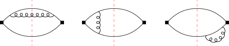
Figure 1: Feynman diagrams for NRQCD matrix elements and shape functions at order $\alpha_{s}$. The filled squares represent $Q\bar{Q}$ bilinear operators, solid lines are heavy quark and antiquark lines, curly lines are gluons, and red vertical dashed lines are final-state cuts. There are also contributions that are obtained by exchanging gluon attachments on a heavy quark line to an antiquark line on the same side of the cut, and by exchanging the left and right sides of the cut. The gauge-completion Wilson line that appears in the color-octet matrix elements and the shape functions is omitted, because diagrams that involve the Wilson line do not appear until two-loop accuracy.

Now we consider the order-$\alpha_{s}$ contributions. At order $\alpha_{s}$, the shape functions are given by the squared amplitudes for $Q\bar{Q}\to Q\bar{Q}$ with a gluon exchange between any of the heavy quark and antiquark lines. The Feynman diagrams for the order-$\alpha_{s}$ contributions are shown in fig. 1. Note that the contribution from the gluon field in $\overleftrightarrow{\bm{D}}$ cancels in the operator definition of the color-singlet shape function, so that there are no diagrams involving direct gluon attachments to the $Q\bar{Q}$ bilinear operator. While same diagrams appear in the order-$\alpha_{s}$ calculation of shape functions and NRQCD matrix elements, contributions from the diagrams where the gluon crosses the final-state cut, like the first diagram in fig. 1, differ between the NRQCD matrix elements and the shape functions, because in the shape functions the momentum component $l_{+}^{*}$ is not integrated over. If both the initial and the final-state $Q\bar{Q}$ are in color-singlet states, such diagrams vanish due to conservation of color. In the case of ${\cal S}_{{}^{3}S_{1}^{[8]}}^{Q\bar{Q}(^{3}S_{1}^{[8]})}(l_{+}^{*})$ and $\langle{\cal O}^{Q\bar{Q}(^{3}S_{1}^{[8]})}(^{3}S_{1}^{[8]})\rangle$, the sum of such diagrams vanish because they involve symmetric linear combinations of the totally antisymmetric $SU(3)$ structure constants. The contributions from the remaining diagrams are same for both the shape function and the NRQCD matrix element. Hence, the tree-level results for ${\cal S}_{{}^{3}P_{0}^{[1]}}^{Q\bar{Q}(^{3}P_{0}^{[1]})}(l_{+}^{*})$ and ${\cal S}_{{}^{3}S_{1}^{[8]}}^{Q\bar{Q}(^{3}S_{1}^{[8]})}(l_{+}^{*})$ hold to order-$\alpha_{s}$ accuracy:

$${\cal S}_{{}^{3}P_{0}^{[1]}}^{Q\bar{Q}(^{3}P_{0}^{[1]})}(l_{+}^{*}) = \delta(l_{+}^{*})\langle{\cal O}^{Q\bar{Q}(^{3}P_{0}^{[1]})}(^{3}P_{0}^{[1]})\rangle+O(\alpha_{s}^{2}),$$ (19a)

$${\cal S}_{{}^{3}S_{1}^{[8]}}^{Q\bar{Q}(^{3}S_{1}^{[8]})}(l_{+}^{*}) = \delta(l_{+}^{*})\langle{\cal O}^{Q\bar{Q}(^{3}S_{1}^{[8]})}(^{3}S_{1}^{[8]})\rangle+O(\alpha_{s}^{2}).$$ (19b)

In the case of ${\cal S}_{{}^{3}P_{0}^{[1]}}^{Q\bar{Q}(^{3}S_{1}^{[8]})}(l_{+}^{*})$, the contribution from the gluon attachment on the heavy quark line cancels the contribution from the gluon attachment on the heavy antiquark line on the same side of the cut. The remaining diagrams cannot produce a color-octet $Q\bar{Q}$ in the final state, and so they do not contribute to ${\cal S}_{{}^{3}P_{0}^{[1]}}^{Q\bar{Q}(^{3}S_{1}^{[8]})}(l_{+}^{*})$. Therefore, the result

$${\cal S}_{{}^{3}P_{0}^{[1]}}^{Q\bar{Q}(^{3}S_{1}^{[8]})}(l_{+}^{*})=0+O(\alpha_{s}^{2}),$$ (20)

holds through order $\alpha_{s}$, and for the same reason, $\langle{\cal O}^{Q\bar{Q}(^{3}S_{1}^{[8]})}(^{3}P_{0}^{[1]})\rangle$ vanishes. While they can become nonzero from corrections of higher orders in $\alpha_{s}$, they will be suppressed by powers of $v$, because they involve dynamical gluons of order $mv$ crossing the cut. Hence, they vanish at current order in $v$.

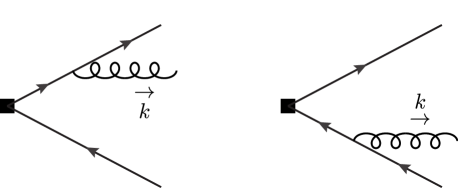
Figure 2: Feynman diagrams for emission of a soft gluon with momentum $k$ from a $Q\bar{Q}$ pair.

The only nontrivial contribution comes from ${\cal S}_{{}^{3}S_{1}^{[8]}}^{Q\bar{Q}(^{3}P_{0}^{[1]})}(l_{+}^{*})$. Similarly to ${\cal S}_{{}^{3}P_{0}^{[1]}}^{Q\bar{Q}(^{3}S_{1}^{[8]})}(l_{+}^{*})$, we only need to consider the diagrams where a gluon crosses the cut, because otherwise the color-octet operator cannot produce a color-singlet $Q\bar{Q}$ in the final state. We set the momenta of the quark and antiquark in the final state to be $(E,\bm{q})$ and $(E,-\bm{q})$, respectively, with $E=\bm{q}^{2}/(2m)$. We use the NRQCD Feynman rules in ref. Bodwin:1998mn . The contributions from gluon attachments to the $Q$ and the $\bar{Q}$ on one side of the cut as shown in fig. 2 involve the factor

$$\frac{ig(\bm{k}+2\bm{q})T^{a}}{2m}\frac{i}{k_{0}+i\varepsilon}+\frac{ig(-\bm{k}+2\bm{q})T^{a}}{2m}\frac{i}{k_{0}+i\varepsilon}=\frac{2ig\bm{q}T^{a}}{m}\frac{i}{k_{0}+i\varepsilon},$$ (21)

where $k$ is the momentum of the gluon, and we neglect the terms $\bm{q}^{2}/(2m)$, $(\bm{q}+\bm{k})^{2}/(2m)$ and $(\bm{q}-\bm{k})^{2}/(2m)$ compared to $k_{0}$ in the heavy quark and antiquark propagators, because they are suppressed by a power of $v$. The product of the factor $\bm{q}$ from the gluon vertices and the Pauli matrix $\bm{\sigma}$ coming from the operator definition of the shape function can be decomposed into the trace, antisymmetric, and traceless symmetric parts as

$$q^{i}\sigma^{j}=\frac{\delta^{ij}}{d-1}\bm{q}\cdot\bm{\sigma}+\frac{q^{i}\sigma^{j}-q^{j}\sigma^{i}}{2}+\left(\frac{q^{i}\sigma^{j}+q^{j}\sigma^{i}}{2}-\frac{\delta^{ij}}{d-1}\bm{q}\cdot\bm{\sigma}\right),$$ (22)

which is valid in $d$ dimensions. In 3 spatial dimensions the three terms correspond to the irreducible angular momentum tensors for total angular momentum 0, 1, and 2. If the $Q\bar{Q}$ in the final state is in the ${}^{3}P_{0}^{[1]}$ state, only the first term survives, and the factor $\bm{q}\cdot\bm{\sigma}$ can be identified as the tree-level matrix element of the $Q\bar{Q}$ bilinear operator $\chi^{\dagger}(-\tfrac{i}{2}\overleftrightarrow{\bm{D}}\cdot\bm{\sigma})\psi$ between the vacuum and the $Q\bar{Q}(^{3}P_{0}^{[1]})$ state. Then, the shape function is given by

$${\cal S}_{{}^{3}S_{1}^{[8]}}^{Q\bar{Q}(^{3}P_{0}^{[1]})}(l_{+}^{*}) = \frac{16\pi\alpha_{s}}{m^{2}}\frac{d-2}{d-1}\frac{C_{F}}{2N_{c}}\langle{\cal O}^{Q\bar{Q}(^{3}P_{0}^{[1]})}(^{3}P_{0}^{[1]})\rangle$$ (23)

$$\times\left(\frac{\Lambda^{2}e^{\gamma_{\rm E}}}{4\pi}\right)^{\frac{4-d}{2}}\int\frac{d^{d}k}{(2\pi)^{d}}\frac{1}{(k_{0}+i\varepsilon)^{2}}2\pi\delta(k^{2})\delta(l_{+}^{*}-k_{+}),$$

where $\Lambda$ is the $\overline{\rm MS}$ scale. Here, the $2\pi\delta(k^{2})$ comes from the gluon crossing the cut, and the $\delta(l_{+}^{*}-k_{+})$ comes from the delta function in the definition of the shape function. The factor $d-2$ comes from the sum over the final-state gluon polarizations, and the factor $1/(d-1)$ comes from the projection onto the ${}^{3}P_{0}^{[1]}$ state. The color factor is computed from $[N_{c}^{-1}{\rm tr}(T^{a}T^{b})]^{2}=T_{F}C_{F}/N_{c}$, with $T_{F}=1/2$. The computation of the integral over $k$ is straightforward: by using $\int d^{d}k=\frac{1}{2}\int dk_{+}dk_{-}d^{d-2}\bm{k}_{\perp}$, we obtain

$${\cal S}_{{}^{3}S_{1}^{[8]}}^{Q\bar{Q}(^{3}P_{0}^{[1]})}(l_{+}^{*})=\frac{4\alpha_{s}C_{F}}{3N_{c}\pi m^{2}}\langle{\cal O}^{Q\bar{Q}(^{3}P_{0}^{[1]})}(^{3}P_{0}^{[1]})\rangle\frac{C_{\epsilon}}{(l_{+}^{*})^{1+2\epsilon}},$$ (24)

where $C_{\epsilon}$ is given by

$$C_{\epsilon}=\frac{(1-\epsilon)(\Lambda^{2}e^{\gamma_{\rm E}})^{\epsilon}\Gamma(1+\epsilon)}{1-\frac{2}{3}\epsilon}.$$ (25)

Expanding $C_{\epsilon}$ in powers of $\epsilon$ to linear order yields $C_{\epsilon}=1+\left(\log\Lambda^{2}-\frac{1}{3}\right)\epsilon+O(\epsilon^{2})$. Equation (24) is the result for the color-octet shape function ${\cal S}_{{}^{3}S_{1}^{[8]}}^{Q\bar{Q}(^{3}P_{0}^{[1]})}(l_{+}^{*})$ valid to order $\alpha_{s}$. Note that we recover the known result for the unrenormalized (bare) color-octet matrix element $\langle{\cal O}^{Q\bar{Q}(^{3}P_{0}^{[1]})}(^{3}S_{1}^{[8]})\rangle^{\rm bare}$ at order $\alpha_{s}$ by integrating over $l_{+}^{*}$:

$$\langle{\cal O}^{Q\bar{Q}(^{3}P_{0}^{[1]})}(^{3}S_{1}^{[8]})\rangle^{\rm bare} = \int_{0}^{\infty}dl_{+}^{*}{\cal S}_{{}^{3}S_{1}^{[8]}}^{Q\bar{Q}(^{3}P_{0}^{[1]})}(l_{+}^{*})$$ (26)

$$= \frac{4\alpha_{s}C_{F}}{3N_{c}\pi m^{2}}\langle{\cal O}^{Q\bar{Q}(^{3}P_{0}^{[1]})}(^{3}P_{0}^{[1]})\rangle\int_{0}^{\infty}dl_{+}^{*}\frac{C_{\epsilon}}{(l_{+}^{*})^{1+2\epsilon}}$$

$$= \frac{4\alpha_{s}C_{F}}{3N_{c}\pi m^{2}}\langle{\cal O}^{Q\bar{Q}(^{3}P_{0}^{[1]})}(^{3}P_{0}^{[1]})\rangle\left(\frac{1}{2\epsilon_{\rm UV}}-\frac{1}{2\epsilon_{\rm IR}}\right).$$

This result also lets us compute the scheme conversion $\Delta(\Lambda,l^{\rm max}_{+})$. From the definition given in eq. (14), we have at order-$\alpha_{s}$ accuracy

$$\Delta(\Lambda,l_{+}^{*\rm max}) = \int_{l_{+}^{*\rm max}}^{\infty}dl_{+}^{*}\frac{4\alpha_{s}C_{F}}{3N_{c}\pi m^{2}}\frac{C_{\epsilon}}{(l_{+}^{*})^{1+2\epsilon}}-\frac{1}{2\epsilon_{\rm UV}}\frac{4\alpha_{s}C_{F}}{3N_{c}\pi m^{2}}$$ (27)

$$= \frac{4\alpha_{s}C_{F}}{3N_{c}\pi m^{2}}\left(\log\Lambda-\log l_{+}^{*\rm max}-\frac{1}{6}\right)+O(\epsilon),$$

which is our result for the scheme conversion in the quarkonium rest frame. Note that this result reproduces the evolution equation in eq. (16). The scheme conversion vanishes at this order if we set $l_{+}^{*\rm max}=\Lambda e^{-1/6}$, that is, $\Delta(\Lambda,l_{+}^{*\rm max}=\Lambda e^{-1/6})=0+O(\alpha_{s}^{2})$, which implies that the cutoff result $\int_{0}^{l_{+}^{*\rm max}}dl_{+}^{*}{\cal S}_{{}^{3}S_{1}^{[8]}}^{\chi_{Q0}}(l_{+}^{*})$ is equal to the $\overline{\rm MS}$-renormalized color-octet matrix element $\langle{\cal O}^{\chi_{Q0}}(^{3}S_{1}^{[8]})\rangle$ at scale $\Lambda=l_{+}^{*\rm max}e^{1/6}$. From $e^{-1/6}\approx 0.85$, we see that the cutoff $l_{+}^{*\rm max}$ is numerically close to the $\overline{\rm MS}$ scale. In phenomenological studies of heavy quarkonium production, the $\overline{\rm MS}$ scale $\Lambda$ for the color-octet matrix element is usually chosen to be the heavy quark mass $m$, and in this case the corresponding cutoff $l_{+}^{*\rm max}$ equals $m\times e^{-1/6}$. Consistently with the assumption that perturbative matching calculations are valid at a suitably chosen factorization scale $\Lambda$, we will also assume that the behavior of the shape function is perturbative for $l_{+}^{*}$ at around or above $l_{+}^{*\rm max}$, so that the $l_{+}^{*}$ dependence of the scheme conversion and the shape function can be described by the perturbative calculation in this section.

We can now explicitly address the boost dependence of $\Delta(\Lambda,l_{+}^{\rm max})$. In a boosted frame, eq. (27) becomes

$$\Delta(\Lambda,l_{+}^{\rm max})\big{|}_{\rm boosted} = \int_{l_{+}^{\rm max}}^{\infty}dl_{+}\frac{4\alpha_{s}C_{F}}{3N_{c}\pi m^{2}}\frac{C_{\epsilon}}{(l_{+})^{1+2\epsilon}}\left(\frac{P_{+}}{P_{+}^{*}}\right)^{2\epsilon}-\frac{1}{2\epsilon_{\rm UV}}\frac{4\alpha_{s}C_{F}}{3N_{c}\pi m^{2}}$$ (28)

$$= \frac{4\alpha_{s}C_{F}}{3N_{c}\pi m^{2}}\left[\log\Lambda-\log\left(l_{+}^{\rm max}\frac{P_{+}^{*}}{P_{+}}\right)-\frac{1}{6}\right]+O(\epsilon),$$

which we obtain by using $l_{+}=(P_{+}/P_{+}^{*})l_{+}^{*}$. The factor $(P_{+}/P_{+}^{*})^{2\epsilon}$ in the integrand is due to the scaling violation of ${\cal S}_{{}^{3}S_{1}^{[8]}}^{Q\bar{Q}(^{3}P_{0}^{[1]})}(l_{+}^{*})$ coming from the $\epsilon$ dependence in $d=4-2\epsilon$ dimensions. Since $l_{+}^{\rm max}\times(P_{+}^{*}/P_{+})=l_{+}^{*\rm max}$, the result is exactly same as $\Delta(\Lambda,l_{+}^{*\rm max})$ computed in the rest frame.

Now that we have the perturbative results for the shape functions valid to order-$\alpha_{s}$ accuracy, the short-distance coefficients $s_{N}$ for the shape function formalism can be obtained at one-loop level from the matching conditions in eqs. (7) by plugging in the results for the shape functions in eqs. (19), (20), and (24). Expressions for the $s_{N}$ in terms of the NRQCD short-distance coefficients $c_{N}$ will be given in section 5.

4 Nonperturbative analysis of shape functions in pNRQCD

The pNRQCD formalism Pineda:1997bj ; Brambilla:1999xf ; Brambilla:2004jw has been proven useful in analyses of inclusive quarkonium production Brambilla:2020ojz ; Brambilla:2021abf ; Brambilla:2022rjd ; Brambilla:2022ayc . This formalism provides expressions for NRQCD matrix elements as products of quarkonium wavefunctions and vacuum expectation values of gluonic operators, and reproduces the known results in terms of quarkonium wavefunctions in the case of color-singlet matrix elements. The vacuum expectation values of gluonic operators, often called gluonic correlators, are defined in terms of Wilson lines and gluon field-strength tensors. Although first-principles calculations of gluonic correlators appearing in NRQCD matrix elements have not yet been done, the fact that they are universal, that is, they are independent of the specific quarkonium state including the heavy quark flavor and radial excitation, significantly enhances the predictive power of the nonrelativistic effective field theory formalism. We refer the readers to refs. Brambilla:2020ojz ; Brambilla:2021abf ; Brambilla:2022rjd ; Brambilla:2022ayc for detailed discussions of pNRQCD calculations of NRQCD matrix elements and phenomenological applications in inclusive quarkonium production.

We can expect to obtain similar results from pNRQCD calculations of shape functions: shape functions can be written in terms of quarkonium wavefunctions and $l_{+}$-dependent gluonic correlators. If the $l_{+}$ dependences are solely contained in the gluonic correlators, then we can expect the $l_{+}$ dependences of the shape functions to be universal among shape functions of quarkonium states that differ by radial excitation or heavy quark flavor. As the model dependence of the shape function formalism comes from the $l_{+}$ dependence of the nonperturbative shape functions, this would greatly enhance the predictive power of the shape function formalism.

In this section, we compute the shape functions ${\cal S}_{{}^{3}P_{0}^{[1]}}^{\chi_{Q0}}(l_{+})$ and ${\cal S}_{{}^{3}S_{1}^{[8]}}^{\chi_{Q0}}(l_{+})$ in the pNRQCD formalism for $P$-wave quarkonium production developed in refs. Brambilla:2020ojz ; Brambilla:2021abf . Similarly to the calculations of NRQCD matrix elements, we will compute them in the quarkonium rest frame as functions of $l_{+}^{*}$. We derive the results nonperturbatively following the development of the formalism in refs. Brambilla:2020ojz ; Brambilla:2021abf , which results in expansions in powers of $v$ and $\Lambda_{\rm QCD}/m$, while the dynamics of the gluon and light quarks are kept nonperturbative. As have been done in refs. Brambilla:2020ojz ; Brambilla:2021abf we assume that the $\chi_{Q}$ states are strongly coupled, so that the scale $mv^{2}$ is smaller than the typical energy gap of gluonic excitations. We will discuss the possibility of extending to the weak coupling case after obtaining the results in the strongly coupled case.

We first briefly review the calculation of NRQCD matrix elements in the formalism developed in refs. Brambilla:2020ojz ; Brambilla:2021abf . In the pNRQCD formalism, the matrix elements are given by

$$\langle{\cal O}^{\cal Q}(N)\rangle = \int d^{d-1}Rd^{d-1}rd^{d-1}r^{\prime}\phi_{\cal Q}(\bm{x}_{1}-\bm{x}_{2})$$ (29)

$$\times\big{[}-V_{{\cal Q}(N)}(\bm{x}_{1},\bm{x}_{2};\bm{\nabla}_{1},\bm{\nabla}_{2})\delta^{(d-1)}(\bm{x}_{1}-\bm{x}_{1}^{\prime})\delta^{(d-1)}(\bm{x}_{2}-\bm{x}_{2}^{\prime})\big{]}$$

$$\times\phi_{\cal Q}^{*}(\bm{x}_{1}^{\prime}-\bm{x}_{2}^{\prime}),$$

where $\phi_{\cal Q}(\bm{x}_{1}-\bm{x}_{2})$ is the wavefunction of the quarkonium ${\cal Q}$ at leading order in $v$, $\bm{x}_{1}$ and $\bm{x}_{2}$ are the positions of the heavy quark and antiquark, respectively, $\bm{r}=\bm{x}_{1}-\bm{x}_{2}$, and $\bm{R}=\frac{1}{2}(\bm{x}_{1}+\bm{x}_{2})$. Similar relations hold for the primed coordinates. The $V_{{\cal Q}(N)}(\bm{x}_{1},\bm{x}_{2};\bm{\nabla}_{1},\bm{\nabla}_{2})$ is a contact term that is determined by matching NRQCD and pNRQCD. The contact terms for the NRQCD matrix elements in eq. (1) are given by

$$-V_{{\cal Q}(^{3}P_{0}^{[1]})}\Big{|}_{P-{\rm wave}} = -\sigma^{i}\otimes\sigma^{j}\frac{N_{c}}{d-1}\nabla_{\bm{r}}^{i}\delta^{(d-1)}(\bm{r})\nabla_{\bm{r}}^{j},$$ (30a)

$$-V_{{\cal Q}(^{3}S_{1}^{[8]})}\Big{|}_{P-{\rm wave}} = -\sigma^{k}\otimes\sigma^{k}N_{c}\nabla_{\bm{r}}^{i}\delta^{(d-1)}(\bm{r})\nabla_{\bm{r}}^{j}\frac{{\cal E}_{11}^{ij}}{N_{c}^{2}m^{2}},$$ (30b)

where we discard contributions that vanish when applied to wavefunctions in $P$-wave states. The tensor ${\cal E}_{11}^{ij}$ is defined by

$${\cal E}_{11}^{ij} = \int_{0}^{\infty}dt\,t\int_{0}^{\infty}dt^{\prime}t^{\prime}\langle\bar{T}\Big{[}\Phi_{\ell}^{{\dagger}ab}(0)\Phi_{0}^{{\dagger}ad}(0,\bm{0};t,\bm{0})gE^{d,i}(t,\bm{0})\Big{]}$$ (31)

$$\hskip 86.11084pt\times T\Big{[}gE^{e,j}(t^{\prime},\bm{0})\Phi_{0}^{ec}(0,\bm{0};t^{\prime},\bm{0})\Phi_{\ell}^{bc}(0)\Big{]}\rangle,$$

where $T$ and $\bar{T}$ indicate time and anti-time orderings of the operators, $E^{a,i}(t,\bm{x})$ is the chromoelectric field at time $t$ and spatial position $\bm{x}$, and $\Phi_{0}(t_{1},\bm{x};t_{2},\bm{x})$ is an adjoint Wilson line in the temporal direction defined by

$$\Phi_{0}(t_{1},\bm{x};t_{2},\bm{x})=P\exp\left[-ig\int_{t_{1}}^{t_{2}}dtA_{0}^{\rm adj}(t,\bm{x})\right].$$ (32)

The configuration of the Wilson lines in the definition of the tensor ${\cal E}_{11}^{ij}$ is shown in fig. 3.

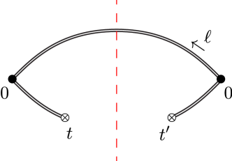
Figure 3: Configuration of the Wilson lines appearing in the definition of the tensor ${\cal E}_{11}^{ij}$ in eq. (31). Filled circles are spacetime origins, double lines are adjoint Wilson lines, red dashed vertical line is the cut, and the crossed circles represent insertions of the chromoelectric field on the temporal Wilson lines at times $t$ and $t^{\prime}$.

Similarly to eq. (22), we can decompose the product $\sigma^{k}\nabla^{i}_{\bm{r}}$ into the trace, antisymmetric, and traceless symmetric parts; if we apply the contact term to a wavefunction in the ${}^{3}P_{0}$ state, the antisymmetric and traceless symmetric parts vanish. Hence, we have

$$-V_{{\cal Q}(^{3}S_{1}^{[8]})}\Big{|}_{{}^{3}P_{0}}=-\sigma^{i}\otimes\sigma^{j}\frac{N_{c}}{d-1}\nabla_{\bm{r}}^{i}\delta^{(d-1)}(\bm{r})\nabla_{\bm{r}}^{j}\frac{{\cal E}_{11}}{(d-1)N_{c}^{2}m^{2}},$$ (33)

where ${\cal E}_{11}$ is the trace of the tensor ${\cal E}_{11}^{ij}$, which can be written as

$${\cal E}_{11}=\int_{0}^{\infty}dt\,t\int_{0}^{\infty}dt^{\prime}t^{\prime}\langle\bar{T}\left[\Phi_{\ell}^{{\dagger}ab}(0)\Phi_{0}^{{\dagger}ad}(0;t)gE^{d,i}(t)\right]T\left[gE^{e,i}(t^{\prime})\Phi_{0}^{ec}(0;t^{\prime})\Phi_{\ell}^{bc}(0)\right]\rangle.$$ (34)

Here we suppress the spatial positions of the operators as they are all evaluated at $\bm{x}=\bm{0}$. The relation between ${\cal E}_{11}$ and the quantity ${\cal E}$ defined in refs. Brambilla:2020ojz ; Brambilla:2021abf is given by ${\cal E}_{11}=\frac{(d-1)N_{c}}{9}{\cal E}$ in $d$ spacetime dimensions. By plugging in the results for the contact terms to the pNRQCD formula in eq. (29), we obtain

$$\langle{\cal O}^{\chi_{Q0}}(^{3}P_{0}^{[1]})\rangle = \frac{3N_{c}}{2\pi}|R^{\prime}(0)|^{2},$$ (35a)

$$\langle{\cal O}^{\chi_{Q0}}(^{3}S_{1}^{[8]})\rangle = \frac{3N_{c}}{2\pi}|R^{\prime}(0)|^{2}\frac{{\cal E}_{11}}{(d-1)N_{c}^{2}m^{2}},$$ (35b)

where $R(r)$ is the radial wavefunction for the $\chi_{Q0}$ state. While the nonperturbative value for ${\cal E}_{11}$ has not yet been computed from first principles, the fact that it is a universal quantity that does not depend on the radial excitation or the heavy quark flavor enhances the predictive power of the nonrelativistic effective field theory formalism. For instance, we have

$$\frac{m^{2}\langle{\cal O}^{\chi_{Q0}}(^{3}S_{1}^{[8]})\rangle}{\langle{\cal O}^{\chi_{Q0}}(^{3}P_{0}^{[1]})\rangle}=\frac{{\cal E}_{11}}{(d-1)N_{c}^{2}},$$ (36)

for any ${}^{3}P_{0}$ quarkonia. Note that ${\cal E}_{11}$ has a logarithmic scale dependence that reproduces the evolution of the color-octet matrix element Brambilla:2020ojz ; Brambilla:2021abf .

We note that the derivatives $\bm{\nabla}_{\bm{r}}$ on the left and right of the $\delta^{(d-1)}(\bm{r})$ in the contact terms in eqs. (30) come from the $Q\bar{Q}$ bilinears on the left and right of the projection operator. Similarly, the two chromoelectric fields in ${\cal E}_{11}$ also come from the $Q\bar{Q}$ bilinears on the left and right of the projection operator. By using these points, it is straightforward to obtain pNRQCD expressions for the shape functions. Rather than working directly with the definitions in eq. (4), we define the Fourier transforms

$$\tilde{\cal S}^{\chi_{Q0}}_{{}^{3}P_{0}^{[1]}}(b_{-}) = \int\frac{dl_{+}^{*}}{4\pi}e^{il^{*}\cdot b}{\cal S}^{\chi_{Q0}}_{{}^{3}P_{0}^{[1]}}(l_{+}^{*})$$ (37a)

$$= \frac{1}{d-1}\langle[\chi^{\dagger}(-\tfrac{i}{2}\overleftrightarrow{\bm{D}}\cdot\bm{\sigma})\psi](x=0){\cal P}_{\chi_{Q0}}[\psi^{\dagger}(-\tfrac{i}{2}\overleftrightarrow{\bm{D}}\cdot\bm{\sigma})\chi](x=b)\rangle,$$

$$\tilde{\cal S}^{\chi_{Q0}}_{{}^{3}S_{1}^{[8]}}(b_{-}) = \int\frac{dl_{+}^{*}}{4\pi}e^{il^{*}\cdot b}{\cal S}^{\chi_{Q0}}_{{}^{3}S_{1}^{[8]}}(l_{+}^{*})$$ (37b)

$$= \langle\big{(}\chi^{\dagger}\sigma^{i}T^{a}\psi\Phi_{\ell}^{{\dagger}ab}\big{)}(x=0){\cal P}_{\chi_{Q0}}\big{(}\Phi_{\ell}^{bc}\psi^{\dagger}\sigma^{i}T^{c}\chi\big{)}(x=b)\rangle,$$

where now the $Q\bar{Q}$ bilinears on the right of the projection operator are displaced by $b$, where $b$ lies in the $-$ direction. The shape functions in momentum space can be recovered from ${\cal S}^{\chi_{Q0}}_{N}(l_{+}^{*})=\int\frac{db_{-}}{2}e^{-il^{*}\cdot b}\tilde{\cal S}^{\chi_{Q0}}_{N}(b_{-})$. Other than that the $Q\bar{Q}$ bilinears on the left and right of the projection operator are computed at different spacetime positions, the pNRQCD calculations of the shape functions are done in the same way as NRQCD matrix elements. We have

$$\tilde{\cal S}_{N}^{\cal Q}(b_{-}) = \int d^{d-1}Rd^{d-1}rd^{d-1}r^{\prime}\phi_{\cal Q}(\bm{x}_{1}-\bm{x}_{2})$$ (38)

$$\times\big{[}-V_{\tilde{\cal S}_{N}}(\bm{x}_{1},\bm{x}_{2};\bm{\nabla}_{1},\bm{\nabla}_{2};b_{-})\delta^{(d-1)}(\bm{x}_{1}-\bm{x}_{1}^{\prime}-\bm{b})\delta^{(d-1)}(\bm{x}_{2}-\bm{x}_{2}^{\prime}-\bm{b})\big{]}$$

$$\times\phi_{\cal Q}^{*}(\bm{x}_{1}^{\prime}-\bm{x}_{2}^{\prime}),$$

where the contact terms for the shape functions acquire dependence on $b_{-}$. The contact terms that survive when acting on wavefunctions in the ${}^{3}P_{0}$ state read

$$-V_{\tilde{\cal S}_{{}^{3}P_{0}^{[1]}}}\Big{|}_{{}^{3}P_{0}} = -\sigma^{i}\otimes\sigma^{j}\frac{N_{c}}{d-1}\nabla_{\bm{r}}^{i}\delta^{(d-1)}(\bm{r})\nabla_{\bm{r}}^{j},$$ (39a)

$$-V_{\tilde{\cal S}_{{}^{3}S_{1}^{[8]}}}\Big{|}_{{}^{3}P_{0}} = -\sigma^{i}\otimes\sigma^{j}\frac{N_{c}}{d-1}\nabla_{\bm{r}}^{i}\delta^{(d-1)}(\bm{r})\nabla_{\bm{r}}^{j}\frac{\tilde{\cal E}\!\!\!/_{11}(b_{-})}{(d-1)N_{c}^{2}m^{2}},$$ (39b)

where

$$\tilde{\cal E}\!\!\!/_{11}(b_{-}) = \int_{0}^{\infty}dt\,t\int_{0}^{\infty}dt^{\prime}t^{\prime}\langle\bar{T}\left[\Phi_{\ell}^{{\dagger}ab}(0)\Phi_{0}^{{\dagger}ad}(0,\bm{0};t,\bm{0})gE^{d,i}(t,\bm{0})\right]$$ (40)

$$\hskip 77.49976pt\times T\left[gE^{e,i}(b_{0}+t^{\prime},\bm{b})\Phi_{0}^{ec}(b_{0},\bm{b};b_{0}+t^{\prime},\bm{b})\Phi_{\ell}^{bc}(b)\right]\rangle.$$

Compared to the expressions for the contact terms for NRQCD matrix elements, the only difference in the shape function formalism is that in $\tilde{\cal E}\!\!\!/_{11}(b_{-})$, the chromoelectric field on the right and the Wilson lines associated with it are displaced by $b$. The displacement does not affect the derivatives $\nabla_{\bm{r}}$, because they only depend on the relative coordinates between the $Q$ and $\bar{Q}$, and they apply to eigenstates of NRQCD. Since the contact term for the color-singlet shape function is independent of $b_{-}$ and is the same as the contact term for the color-singlet NRQCD matrix element, we have

$$\tilde{\cal S}^{\chi_{Q0}}_{{}^{3}P_{0}^{[1]}}(b_{-})=\langle{\cal O}^{\chi_{Q0}}(^{3}P_{0}^{[1]})\rangle,$$ (41)

which implies

$${\cal S}^{\chi_{Q0}}_{{}^{3}P_{0}^{[1]}}(l_{+})=\delta(l_{+})\langle{\cal O}^{\chi_{Q0}}(^{3}P_{0}^{[1]})\rangle.$$ (42)

On the other hand, the Fourier transformed color-octet shape function acquires dependence on $b_{-}$ through $\tilde{\cal E}\!\!\!/_{11}(b_{-})$, so that

$$\tilde{\cal S}_{{}^{3}S_{1}^{[8]}}^{\chi_{Q0}}(b_{-})=\frac{3N_{c}}{2\pi}|R^{\prime}(0)|^{2}\frac{\tilde{\cal E}\!\!\!/_{11}(b_{-})}{(d-1)N_{c}^{2}m^{2}}.$$ (43)

Then the shape function can be written as

$${\cal S}_{{}^{3}S_{1}^{[8]}}^{\chi_{Q0}}(l_{+}^{*})=\frac{3N_{c}}{2\pi}|R^{\prime}(0)|^{2}\frac{{\cal E}\!\!\!/_{11}(l_{+}^{*})}{(d-1)N_{c}^{2}m^{2}},$$ (44)

where

$${\cal E}\!\!\!/_{11}(l_{+}^{*})=\int\frac{db_{-}}{2}e^{-il^{*}\cdot b}\tilde{\cal E}\!\!\!/_{11}(b_{-}).$$ (45)

Similarly to the case of NRQCD matrix elements, the quantity ${\cal E}\!\!\!/_{11}(l_{+})$ is universal, and do not depend on the radial excitation or the heavy quark flavor of the quarkonium state. In particular, we have

$$\frac{m^{2}{\cal S}_{{}^{3}S_{1}^{[8]}}^{\chi_{Q0}}(l_{+}^{*})}{\langle{\cal O}^{\chi_{Q0}}(^{3}P_{0}^{[1]})\rangle}=\frac{{\cal E}\!\!\!/_{11}(l_{+}^{*})}{(d-1)N_{c}^{2}},$$ (46)

which is valid for any ${}^{3}P_{0}$ quarkonia. This, together with heavy quark spin symmetry, implies that the $l_{+}$ dependence of the color octet shape function is universal for all $P$-wave heavy quarkonia, including all radial excitations of $\chi_{c}$ and $\chi_{b}$. This significantly reduces the model dependence in the phenomenological analysis of $\chi_{c}$ and $\chi_{b}$ production in the shape function formalism.

An important consistency check of the pNRQCD calculation is to compare the result with the perturbative calculation. If we compute ${\cal E}\!\!\!/_{11}(l_{+}^{*})$ in perturbative QCD at leading nonvanishing order in $\alpha_{s}$, we obtain

$${\cal E}\!\!\!/_{11}(l_{+}^{*})|_{\rm pQCD} = 4\pi\alpha_{s}(d-2)(N_{c}^{2}-1)\mu^{2\epsilon}\int_{0}^{\infty}dt\,t\int_{0}^{\infty}dt^{\prime}\,t^{\prime}$$ (47)

$$\times\int\frac{db_{-}}{2}e^{-il^{*}\cdot b}\int\frac{d^{d}k}{(2\pi)^{d}}\frac{i\bm{k}^{2}}{k^{2}+i\varepsilon}e^{ik\cdot b}e^{ik_{0}(t-t^{\prime})}+O(\alpha_{s}^{2})$$

$$= 4\pi\alpha_{s}(d-2)(N_{c}^{2}-1)\mu^{2\epsilon}\int\frac{d^{d-1}k}{(2\pi)^{d-1}}\frac{1}{2|\bm{k}|^{3}}\delta(k_{+}-l_{+}^{*})+O(\alpha_{s}^{2})$$

$$= \alpha_{s}(d-2)(N_{c}^{2}-1)\mu^{2\epsilon}\int\frac{d^{d-2}\bm{k}_{\perp}}{(2\pi)^{d-2}l_{+}^{*}}\frac{1}{(l_{+}^{*}-\bm{k}_{\perp}^{2}/l_{+}^{*})^{2}/4+\bm{k}_{\perp}^{2}}+O(\alpha_{s}^{2})$$

$$= \frac{(d-1)C_{\epsilon}}{3}\frac{4\alpha_{s}C_{F}N_{c}}{\pi(l_{+}^{*})^{1+2\epsilon}}+O(\alpha_{s}^{2}),$$

where $C_{\epsilon}$ is defined in eq. (25). By plugging in this expression into the pNRQCD expression for the shape function (44) and using $\langle{\cal O}^{\chi_{Q0}}(^{3}P_{0}^{[1]})\rangle=\frac{3N_{c}}{2\pi}|R^{\prime}(0)|^{2}$ we obtain

$${\cal S}_{{}^{3}S_{1}^{[8]}}^{\chi_{Q0}}(l_{+})\Big{|}_{\rm pQCD}=\langle{\cal O}^{\chi_{Q0}}(^{3}P_{0}^{[1]})\rangle\left(\frac{4\alpha_{s}C_{F}}{3N_{c}m^{2}\pi}\frac{C_{\epsilon}}{(l_{+}^{*})^{1+2\epsilon}}+O(\alpha_{s}^{2})\right),$$ (48)

which exactly reproduces the order-$\alpha_{s}$ calculation of ${\cal S}_{{}^{3}S_{1}^{[8]}}^{Q\bar{Q}(^{3}P_{0}^{[1]})}(l_{+})$ in the previous section, demonstrating the validity of the pNRQCD result at one-loop level. This is also consistent with the result for the scheme conversion $\Delta(\Lambda,l_{+}^{*\rm max}=\Lambda e^{-1/6})=0+O(\alpha_{s}^{2})$, so that we have

$$\int_{0}^{l_{+}^{*\rm max}}dl_{+}^{*}{\cal S}_{{}^{3}S_{1}^{[8]}}^{\chi_{Q0}}(l_{+}^{*})\Big{|}_{l_{+}^{*\rm max}=\Lambda e^{-1/6}}=\langle{\cal O}^{\chi_{Q0}}({}^{3}S_{1}^{[8]})\rangle^{\overline{\rm MS}}.$$ (49)

As have been discussed in section 3, the UV divergence on the left-hand side is regulated by the cutoff $l_{+}^{*\rm max}$, so that the nonperturbative shape function ${\cal S}_{{}^{3}S_{1}^{[8]}}^{\chi_{Q0}}(l_{+}^{*})$ can be computed in $d=4$ dimensions. This allows us to use the UV-regulated normalization condition to constrain the model dependence of the nonperturbative shape function.

So far the pNRQCD calculations of the NRQCD matrix elements and shape functions presented in this section were based on the assumption that the $\chi_{Q0}$ state is strongly coupled, so that the ultrasoft scale, where the gluons have energies and momenta of order $mv^{2}$, does not play a role. In the weakly coupled case, the chromoelectric dipole interaction will mix color-singlet and color-octet $Q\bar{Q}$ states through exchange of ultrasoft gluons, so that the contribution from the color-octet wavefunction must be included. As have been discussed in refs. Beneke:1999zr ; Beneke:2013jia , this interaction is suppressed by $v^{3/2}$ compared to the kinetic terms in the pNRQCD Lagrangian, so that for heavy quarkonium states, the contribution from the color-octet wavefunction is suppressed by $v^{3}$ compared to the color-singlet part. The color-octet wavefunction can appear in the color-octet NRQCD matrix element and the shape function through the contact terms at leading order in $1/m$, which is enhanced by $1/v^{2}$ compared to the contact terms that act on the color-singlet wavefunction [eqs. (30) and (39)]. As a result, in the weak coupling case, the extra contribution coming from the color-octet wavefunction is suppressed by at least a power of $v$ compared to the pNRQCD expressions for NRQCD matrix elements and shape functions in the strongly coupled case. Hence, we expect the pNRQCD results obtained in this section to also hold in the weakly coupled case at leading nonvanishing order in $v$.

5 One-loop matching conditions

Based on the calculations of the perturbative shape functions, we now derive the matching conditions that allow determination of the short-distance coefficients $s_{N}$ for the shape function formalism.

As have been discussed in section 2, the matching coefficients are computed from the cross sections for inclusive production of $Q\bar{Q}$ in specific color and angular momentum states. The cross section for production of $Q\bar{Q}$ in the ${}^{3}S_{1}^{[8]}$ state [eqs. (6b) and (7b)] gives the following matching condition

$$c_{{}^{3}S_{1}^{[8]}}(P)\langle{\cal O}^{Q\bar{Q}(^{3}S_{1}^{[8]})}(^{3}S_{1}^{[8]})\rangle = \int_{0}^{\infty}dl_{+}\,s_{{}^{3}S_{1}^{[8]}}(P+l){\cal S}_{{}^{3}S_{1}^{[8]}}^{Q\bar{Q}(^{3}S_{1}^{[8]})}(l_{+})$$ (50)

$$= s_{{}^{3}S_{1}^{[8]}}(P)\langle{\cal O}^{Q\bar{Q}(^{3}S_{1}^{[8]})}(^{3}S_{1}^{[8]})\rangle.$$

In the last line, we used the one-loop result for the perturbative shape function in eq. (19). This implies that $s_{{}^{3}S_{1}^{[8]}}(P)=c_{{}^{3}S_{1}^{[8]}}(P)$ holds at one-loop level. Similarly, expressions for the ${}^{3}P_{J}^{[1]}$ production cross section [eqs. (6a) and (7a)] give

$$c_{{}^{3}P_{J}^{[1]}}(P)\langle{\cal O}^{Q\bar{Q}(^{3}P_{0}^{[1]})}(^{3}P_{0}^{[1]})\rangle+c_{{}^{3}S_{1}^{[8]}}(P)\langle{\cal O}^{Q\bar{Q}(^{3}P_{0}^{[1]})}(^{3}S_{1}^{[8]})\rangle$$ (51)

$$= \int_{0}^{\infty}dl_{+}\left[s_{{}^{3}P_{J}^{[1]}}(P+l){\cal S}_{{}^{3}P_{0}^{[1]}}^{Q\bar{Q}(^{3}P_{0}^{[1]})}(l_{+})+s_{{}^{3}S_{1}^{[8]}}(P+l){\cal S}_{{}^{3}S_{1}^{[8]}}^{Q\bar{Q}(^{3}P_{0}^{[1]})}(l_{+})\right]$$

$$= s_{{}^{3}P_{J}^{[1]}}(P)\langle{\cal O}^{Q\bar{Q}(^{3}P_{0}^{[1]})}(^{3}P_{0}^{[1]})\rangle+\int_{0}^{\infty}dl_{+}c_{{}^{3}S_{1}^{[8]}}(P+l){\cal S}_{{}^{3}S_{1}^{[8]}}^{Q\bar{Q}(^{3}P_{0}^{[1]})}(l_{+}),$$

where the first line is the NRQCD expression divided by $2J+1$, and the last line follows from the result for the perturbative shape function in eq. (19) and the result $s_{{}^{3}S_{1}^{[8]}}(P)=c_{{}^{3}S_{1}^{[8]}}(P)$. In principle, we can obtain expressions for $s_{{}^{3}P_{J}^{[1]}}(P)$ in terms of $c_{{}^{3}P_{J}^{[1]}}(P)$ and $c_{{}^{3}S_{1}^{[8]}}(P)$ by plugging in the perturbative expressions for $\langle{\cal O}^{Q\bar{Q}(^{3}P_{0}^{[1]})}(^{3}S_{1}^{[8]})\rangle$ and ${\cal S}_{{}^{3}S_{1}^{[8]}}^{Q\bar{Q}(^{3}P_{0}^{[1]})}(l_{+})$. However, the resulting expression is not very useful, because the matrix element $\langle{\cal O}^{Q\bar{Q}(^{3}P_{0}^{[1]})}(^{3}S_{1}^{[8]})\rangle$ contains an IR pole, and hence, the NRQCD side of the expression depends on the order-$\epsilon$ contribution to the short-distance coefficient $c_{{}^{3}S_{1}^{[8]}}(P)$ that is usually not available. The same IR pole that matches the one on the NRQCD side of the expression does appear on the shape function formalism side, which arises from the integral in the last line of eq. (51) in the region $l_{+}\to 0$. Hence, the terms involving IR poles on both sides can be matched exactly if we rewrite this integral as

$$\int_{0}^{\infty}dl_{+}c_{{}^{3}S_{1}^{[8]}}(P+l){\cal S}_{{}^{3}S_{1}^{[8]}}^{Q\bar{Q}(^{3}P_{0}^{[1]})}(l_{+}) = \int_{0}^{\infty}dl_{+}\left(c_{{}^{3}S_{1}^{[8]}}(P+l)-c_{{}^{3}S_{1}^{[8]}}(P)\right){\cal S}_{{}^{3}S_{1}^{[8]}}^{Q\bar{Q}(^{3}P_{0}^{[1]})}(l_{+})$$ (52)

$$+c_{{}^{3}S_{1}^{[8]}}(P)\langle{\cal O}^{Q\bar{Q}(^{3}P_{0}^{[1]})}(^{3}S_{1}^{[8]})\rangle^{\rm bare},$$

where the unrenormalized (“bare”) matrix element is given by eq. (26). Note that the integral over $l_{+}$ on the right-hand side is IR finite because the integrand factor in the parenthesis vanishes as $l_{+}\to 0$, and the only IR pole is isolated in the perturbative color-octet matrix element. This expression is still not completely satisfactory, because NRQCD matching calculations are usually done in the $\overline{\rm MS}$ scheme, while the above expression involves an unrenormalized matrix element. Rather than subtracting the pole to carry out the renormalization in the $\overline{\rm MS}$ scheme, we can use the result for $\Delta(\Lambda,l_{+}^{\rm max})$ we obtained earlier in eq. (27) to cut off the UV-divergent integral. By using eqs. (15) and (27), we have at one-loop level

$$\int_{0}^{\infty}dl_{+}\theta(l_{+}^{\rm max}-l_{+}){\cal S}_{{}^{3}S_{1}^{[8]}}^{Q\bar{Q}(^{3}P_{0}^{[1]})}(l_{+})\Big{|}_{l_{+}^{*\rm max}=\Lambda e^{-1/6}}=\langle{\cal O}^{Q\bar{Q}(^{3}P_{0}^{[1]})}(^{3}S_{1}^{[8]})\rangle^{\overline{\rm MS}},$$ (53)

where $\theta(x)$ is the step function that vanishes for $x<0$ and equals $1$ for $x\geq 0$, and $\Lambda$ is the $\overline{\rm MS}$ renormalization scale for the color-octet matrix element $\langle{\cal O}^{Q\bar{Q}(^{3}P_{0}^{[1]})}(^{3}S_{1}^{[8]})\rangle$. By using this we can rewrite the color-octet shape-function term in the matching condition as

$$\int_{0}^{\infty}dl_{+}c_{{}^{3}S_{1}^{[8]}}(P+l){\cal S}_{{}^{3}S_{1}^{[8]}}^{Q\bar{Q}(^{3}P_{0}^{[1]})}(l_{+})=c_{{}^{3}S_{1}^{[8]}}(P)\langle{\cal O}^{Q\bar{Q}(^{3}P_{0}^{[1]})}(^{3}S_{1}^{[8]})\rangle^{\overline{\rm MS}}$$

$$+\int_{0}^{\infty}dl_{+}\left(c_{{}^{3}S_{1}^{[8]}}(P+l)-c_{{}^{3}S_{1}^{[8]}}(P)\theta(l_{+}^{\rm max}-l_{+})\right){\cal S}_{{}^{3}S_{1}^{[8]}}^{Q\bar{Q}(^{3}P_{0}^{[1]})}(l_{+}),$$ (54)

where now every term is UV finite, and the IR pole is isolated in the $\overline{\rm MS}$-renormalized matrix element at the scale $\Lambda=l_{+}^{*\rm max}e^{1/6}$. By plugging this expression to eq. (51) we obtain

$$c_{{}^{3}P_{J}^{[1]}}^{\overline{\rm MS}}(P)\langle{\cal O}^{Q\bar{Q}(^{3}P_{0}^{[1]})}(^{3}P_{0}^{[1]})\rangle+c_{{}^{3}S_{1}^{[8]}}(P)\langle{\cal O}^{Q\bar{Q}(^{3}P_{0}^{[1]})}(^{3}S_{1}^{[8]})\rangle^{\overline{\rm MS}}$$ (55)

$$= s_{{}^{3}P_{J}^{[1]}}(P)\langle{\cal O}^{Q\bar{Q}(^{3}P_{0}^{[1]})}(^{3}P_{0}^{[1]})\rangle+c_{{}^{3}S_{1}^{[8]}}(P)\langle{\cal O}^{Q\bar{Q}(^{3}P_{0}^{[1]})}(^{3}S_{1}^{[8]})\rangle^{\overline{\rm MS}}$$

$$+\int_{0}^{\infty}dl_{+}\left(c_{{}^{3}S_{1}^{[8]}}(P+l)-c_{{}^{3}S_{1}^{[8]}}(P)\theta(l_{+}^{\rm max}-l_{+})\right){\cal S}_{{}^{3}S_{1}^{[8]}}^{Q\bar{Q}(^{3}P_{0}^{[1]})}(l_{+}).$$

If we solve this for $s_{{}^{3}P_{J}^{[1]}}(P)$, the terms involving IR poles from the color-octet matrix element cancel exactly, so everything can be computed at $d=4$. By using the result for ${\cal S}_{{}^{3}S_{1}^{[8]}}^{Q\bar{Q}(^{3}P_{0}^{[1]})}(l_{+})$ in eq. (24), we obtain

$$s_{{}^{3}P_{J}^{[1]}}(P)=c_{{}^{3}P_{J}^{[1]}}^{\overline{\rm MS}}(P)-\left(c_{{}^{3}P_{J}^{[1]}}^{\rm singular}(P)-c_{{}^{3}P_{J}^{[1]}}^{\rm pole}(P)\right),$$ (56)

where

$$c_{{}^{3}P_{J}^{[1]}}^{\rm singular}(P) = \frac{4\alpha_{s}C_{F}}{3N_{c}\pi m^{2}}\int_{0}^{\infty}dl_{+}c_{{}^{3}S_{1}^{[8]}}(P+l)\frac{C_{\epsilon}(P_{+}/P_{+}^{*})^{2\epsilon}}{l_{+}^{1+2\epsilon}},$$ (57a)

$$c_{{}^{3}P_{J}^{[1]}}^{\rm pole}(P) = \frac{4\alpha_{s}C_{F}}{3N_{c}\pi m^{2}}c_{{}^{3}S_{1}^{[8]}}(P)\int_{0}^{l_{+}^{\rm max}}dl_{+}\frac{C_{\epsilon}(P_{+}/P_{+}^{*})^{2\epsilon}}{l_{+}^{1+2\epsilon}}.$$ (57b)

The labels “singular” and “pole” will be explained later. Since the poles cancel in the last line of eq. (55), the $\epsilon$ dependences in $c_{{}^{3}S_{1}^{[8]}}$ can be dropped. By using this result for $s_{{}^{3}P_{J}^{[1]}}(P)$ we can now write the cross section in the shape function formalism as

$$\sigma[{\chi_{QJ}(P)}]_{\rm shape}=(2J+1)\bigg{[}s_{{}^{3}P_{J}^{[1]}}(P)\langle{\cal O}^{\chi_{Q0}}(^{3}P_{0}^{[1]})\rangle+\int_{0}^{\infty}dl_{+}c_{{}^{3}S_{1}^{[8]}}(P+l){\cal S}_{{}^{3}S_{1}^{[8]}}^{\chi_{Q0}}(l_{+})\Big{|}_{\rm NP}\bigg{]},$$ (58)

where $s_{{}^{3}P_{J}^{[1]}}(P)$ is given in eq. (56), and ${\cal S}_{{}^{3}S_{1}^{[8]}}^{\chi_{Q0}}(l_{+})\big{|}_{\rm NP}$ is the nonperturbative color-octet shape function.

The expression for $s_{{}^{3}P_{J}^{[1]}}(P)$ in eq. (56) calls for further exploration. We show that the term $c_{{}^{3}P_{J}^{[1]}}^{\rm singular}(P)$ is essentially the singular contribution to the $Q\bar{Q}(^{3}P_{J}^{[1]})$ cross section that occurs through the production of $Q\bar{Q}(^{3}S_{1}^{[8]})$, which then evolves into a $P$-wave color-singlet $Q\bar{Q}$ by emitting a soft gluon. The soft gluon emission amplitude from a heavy quark line with momentum $p_{1}$ is given by

$$\bar{u}(p_{1})ig\gamma^{\mu}T^{a}\frac{i(p\!\!\!/_{1}+k\!\!\!/+m)}{k^{2}+2k\cdot p_{1}+i\varepsilon}\approx\bar{u}(p_{1})ig\gamma^{\mu}T^{a}\frac{i(p\!\!\!/_{1}+m)}{2k\cdot p_{1}+i\varepsilon}=-g\bar{u}(p_{1})T^{a}\frac{p_{1}^{\mu}}{k\cdot p_{1}+i\varepsilon},$$ (59)

where we retained only the leading contribution in the limit where $k$ is soft, and in the last equality we anticommuted $p\!\!\!/_{1}$ to the left and used the equation of motion. Similarly, the infrared divergent contribution coming from the heavy antiquark line with momentum $p_{2}$ is given by

$$\frac{i(-p\!\!\!/_{2}-k\!\!\!/+m)}{k^{2}+2k\cdot p_{2}+i\varepsilon}ig\gamma^{\mu}T^{a}v(p_{2})\approx\frac{i(-p\!\!\!/_{2}+m)}{2k\cdot p_{2}+i\varepsilon}ig\gamma^{\mu}T^{a}v(p_{2})=+g\frac{p_{2}^{\mu}}{k\cdot p_{2}+i\varepsilon}T^{a}v(p_{2}).$$ (60)

Hence, the soft-gluon emission gives rise to an infrared divergent contribution that is given by $\sigma[Q\bar{Q}(^{3}S_{1}^{[8]})(p_{1}+p_{2}+k)]$ times the factor

$$-g\left(\frac{p_{1}^{\mu}}{k\cdot p_{1}+i\varepsilon}-\frac{p_{2}^{\mu}}{k\cdot p_{2}+i\varepsilon}\right)T^{a}$$ (61)

multiplied on both sides of the cut, and integrated over the phase space of the soft gluon. We can see that this soft gluon factor is proportional to $1/|\bm{k}|$, so that the phase space integral involves the singular integral $\int d^{d-1}k\,|\bm{k}|^{-3}$. After a straightforward calculation, at leading nonvanishing order in expansion in powers of $q=(p_{1}-p_{2})/2$ compared to $p_{1}+p_{2}$, the singular contribution to the $Q\bar{Q}(^{3}P_{J}^{[1]})$ cross section is given by

$$(2J+1)\langle{\cal O}^{Q\bar{Q}(^{3}P_{0}^{[1]})}(^{3}P_{0}^{[1]})\rangle\left(\frac{4\pi\alpha_{s}C_{F}}{3N_{c}\pi m^{2}}\int_{0}^{\infty}\frac{d|\bm{k}|}{|\bm{k}|^{1+2\epsilon}}c_{{}^{3}S_{1}^{[8]}}(P+k)+O(\epsilon^{0})\right),$$ (62)

which, aside from an order-$\epsilon^{0}$ finite piece, matches exactly the contribution from the $c_{{}^{3}P_{J}^{[1]}}^{\rm singular}(P)$ term. This term does not have a UV divergence, because $c_{{}^{3}S_{1}^{[8]}}(P+l)$ vanishes when $l$ is sufficiently large, but it does have an IR pole coming from the region $l_{+}\to 0$. This IR pole is canceled exactly by the term $c_{{}^{3}P_{J}^{[1]}}^{\rm pole}(P)$, which can be computed as

$$c_{{}^{3}P_{J}^{[1]}}^{\rm pole}(P)=\frac{4\alpha_{s}C_{F}}{3N_{c}\pi m^{2}}c_{{}^{3}S_{1}^{[8]}}(P)\left(-\frac{1}{2\epsilon_{\rm IR}}\right)+O(\epsilon),$$ (63)

where we set $l_{+}^{*\rm max}=\Lambda e^{-1/6}$. Hence, the term $c_{{}^{3}P_{J}^{[1]}}^{\rm pole}(P)$ subtracts exactly the IR pole in $c_{{}^{3}P_{J}^{[1]}}^{\rm singular}(P)$. Note that in practical calculations, $c_{{}^{3}P_{J}^{[1]}}^{\overline{\rm MS}}$ is obtained by first computing the IR-divergent $Q\bar{Q}(^{3}P_{J}^{[1]})$ cross section, and then subtracting the IR pole. As the same thing happens in the combination $c_{{}^{3}P_{J}^{[1]}}^{\rm singular}(P)-c_{{}^{3}P_{J}^{[1]}}^{\rm pole}(P)$, this is essentially the singular soft-gluon contribution in $c_{{}^{3}P_{J}^{[1]}}^{\overline{\rm MS}}(P)$. That is, the second term in eq. (56) subtracts the singular soft-gluon emission contribution from the NRQCD short-distance coefficient $c_{{}^{3}P_{J}^{[1]}}^{\overline{\rm MS}}$. Note that this identification still holds at higher orders in $\alpha_{s}$ when radiative corrections are included in $c_{{}^{3}S_{1}^{[8]}}(P+l)$ and $c_{{}^{3}S_{1}^{[8]}}(P)$, because once the color-octet $Q\bar{Q}$ evolves into a color-singlet state by emission of soft gluons, the color-singlet $Q\bar{Q}$ no longer emits soft gluons unless corrections of higher orders in $v$ are included, as we have seen in the calculation of the matrix elements and shape functions in the previous section.

The soft-gluon emission that is subtracted from the color-singlet short-distance coefficient instead appears in the color-octet shape function contribution, where the nonperturbative effect of the soft gluon emission is encoded in the shape function. To see this explicitly, we can rewrite the color-octet shape function term in the cross section formula (58) as

$$\int_{0}^{\infty}dl_{+}c_{{}^{3}S_{1}^{[8]}}(P+l){\cal S}_{{}^{3}S_{1}^{[8]}}^{\chi_{Q0}}(l_{+})\Big{|}_{\rm NP}=c_{{}^{3}S_{1}^{[8]}}(P)\langle{\cal O}^{\chi_{Q0}}(^{3}S_{1}^{[8]})\rangle^{\overline{\rm MS}}$$ (64)

$$+\int_{0}^{\infty}dl_{+}\left(c_{{}^{3}S_{1}^{[8]}}(P+l)-c_{{}^{3}S_{1}^{[8]}}(P)\theta(l_{+}^{\rm max}-l_{+})\right){\cal S}_{{}^{3}S_{1}^{[8]}}^{\chi_{Q0}}(l_{+})\Big{|}_{\rm NP}.$$

We see that the second term in eq. (56) is equivalent to the last line of the above expression, with an opposite sign and the shape function replaced by its large-$l_{+}$ asymptotic behavior given in eq. (10). By using this we can rewrite eq. (58) as

$$\sigma[{\chi_{QJ}(P)}]_{\rm shape} = (2J+1)\bigg{[}c_{{}^{3}P_{J}^{[1]}}^{\overline{\rm MS}}(P)\langle{\cal O}^{\chi_{Q0}}(^{3}P_{0}^{[1]})\rangle+c_{{}^{3}S_{1}^{[8]}}(P)\langle{\cal O}^{\chi_{Q0}}(^{3}S_{1}^{[8]})\rangle^{\overline{\rm MS}}$$ (65)

$$\hskip 43.05542pt+\int_{0}^{\infty}dl_{+}\left(c_{{}^{3}S_{1}^{[8]}}(P+l)-c_{{}^{3}S_{1}^{[8]}}(P)\theta(l_{+}^{\rm max}-l_{+})\right)$$

$$\hskip 94.72192pt\times\Big{(}{\cal S}_{{}^{3}S_{1}^{[8]}}^{\chi_{Q0}}(l_{+})\Big{|}_{\rm NP}-{\cal S}_{{}^{3}S_{1}^{[8]}}^{\chi_{Q0}}(l_{+})\Big{|}_{\rm asy}\Big{)}\bigg{]}.$$

Here, the first line is just the cross section in NRQCD, while the remaining terms arise from the deviation of the nonperturbative shape function from its asymptotic form. That is, the integral over $l_{+}$ in eq. (65) encode the nonperturbative corrections to the NRQCD factorization formalism that arise from resummation of kinematical effects from the motion of $Q\bar{Q}$ relative to the quarkonium.

Although eqs. (58) and (65) are in principle equivalent expressions for the $\chi_{QJ}$ production cross section in the shape function formalism, they have different phenomenological implications, as we will now briefly describe. In order to compute cross sections from eq. (58), the short-distance coefficient $s_{{}^{3}P_{J}^{[1]}}(P)$ must be determined from eq. (56). Note that at one-loop level, the NRQCD short-distance coefficient $c_{{}^{3}P_{J}^{[1]}}(P)$ contains the soft-gluon contribution given by the second term in eq. (56). This soft-gluon effect generates a logarithm of the $\overline{\rm MS}$ scale in $c_{{}^{3}P_{J}^{[1]}}$, which is canceled by the scale dependence of the color-octet matrix element times $c_{{}^{3}S_{1}^{[8]}}$ at tree level. However, since usually in NRQCD calculations both the color-singlet and color-octet short-distance coefficients are computed to same accuracy in $\alpha_{s}$, there is always a mismatch of the orders in $\alpha_{s}$ of soft-gluon effects between the color-singlet and color-octet channels, due to the one-loop correction included in $c_{{}^{3}S_{1}^{[8]}}$. This mismatch can have a significant effect, as the soft gluon emission involves IR divergences which make the cross sections singular near threshold. If we use eq. (58) to compute $\chi_{QJ}$ cross sections, this singular contribution is subtracted from the ${}^{3}P_{J}^{[1]}$ short-distance coefficient, and added back to the second term in the square brackets of eq. (58) in the form of eq. (64). In this way, the singular soft-gluon emission effects are contained entirely in the color-octet shape function contribution in the form given in eq. (64), where the short-distance coefficient $c_{{}^{3}S_{1}^{[8]}}$ can now be computed to same order in $\alpha_{s}$ for every term. This allows the singular soft-gluon emission effects to be computed to consistent accuracy in $\alpha_{s}$. Note that, since the integral over $l_{+}$ in eq. (64) is infrared finite even when the nonperturbative shape function is replaced by its asymptotic form, this matching of singular soft-gluon effects can be done without knowledge of the nonperturbative form of ${\cal S}_{{}^{3}S_{1}^{[8]}}^{\chi_{Q0}}(l_{+})$. We will investigate this point in more detail in section 6.1.

The form of the cross section given in eq. (65) is suitable for computing the nonperturbative corrections to the NRQCD factorization formalism from the nonperturbative shape function. We note that if we were to neglect the deviation of the nonperturbative shape function from its asymptotic form, the last line of eq. (65) vanishes and we recover the cross section in NRQCD factorization. This is consistent with the fact that, if the color-octet shape function is given by the asymptotic form in eq. (10), all of the higher-dimensional matrix elements in eq. (3b) are proportional to scaleless power divergences $\int_{0}^{\infty}dl_{+}\,l_{+}^{n-1}$ for $n\geq 1$, which vanish in dimensional regularization (in the case of higher-dimensional color-singlet matrix elements, they vanish in the form $\int_{0}^{\infty}dl_{+}\,l_{+}^{n}\delta(l_{+})=0$). The nonperturbative corrections to the $p_{T}$-differential cross sections coming from the last two lines in eq. (65) will be computed in section 6.2 using models for the nonperturbative shape functions, which are constrained by the asymptotic form (10) and the normalization condition given by eq. (49).

6 Phenomenological applications

Based on the one-loop level matching conditions and the shape functions we have established in the previous sections, we compute $\chi_{c}$ and $\chi_{b}$ cross sections in the shape function formalism and compare the results with NRQCD predictions. As we have explained in sec. 1, understanding the $\chi_{c}$ and $\chi_{b}$ cross sections are not only important for comparing predictions with cross section measurements in experiment, but they are also important for correctly treating the feeddown contributions in $S$-wave production rates. We will show in this section that the shape function formalism can modify the transverse-momentum dependent cross sections of $P$-wave heavy quarkonia, which may have important implications in heavy quarkonium production phenomenology.

6.1 Matching of soft-gluon emission effects at large transverse momentum

We first investigate the phenomenological application of the cross section formula in eq. (58) for mixing of soft-gluon emission effects between color-singlet and color-octet channels. Since the effects of soft-gluon emission near threshold is most prominent at large $p_{T}$, we consider the cross section in the fragmentation approximation, which describes the cross section at leading power in the expansion in powers of $m^{2}/p_{T}^{2}$ Collins:1981uw . In this approximation, the cross section is given by

$$\sigma[\chi_{QJ}(P)]=\sum_{i=g,q,\bar{q}}\int dz\,\hat{\sigma}_{i}(k)D_{i\to\chi_{QJ}+X}(z),$$ (66)

where the sum is over gluon, light quarks and antiquarks, $\hat{\sigma}_{i}(k)$ is the production rate of a parton $i$ with momentum $k$, $D_{i\to\chi_{QJ}}(z)$ is the fragmentation function, which is a function of the momentum fraction $z=P_{+}/k_{+}$, with the $+$ direction defined along the quarkonium momentum. For notational convenience, we will write the parton cross section $\hat{\sigma}_{i}$ as a function of $z$. The NRQCD factorization formula for the fragmentation function reads

$$D_{i\to\chi_{cJ}+X}(z)=(2J+1)\left[d_{i\to{}^{3}S_{1}^{[8]}}(z)\langle{\cal O}^{\chi_{Q0}}(^{3}S_{1}^{[8]})\rangle+d_{i\to{}^{3}P_{J}^{[1]}}(z)\langle{\cal O}^{\chi_{Q0}}(^{3}P_{J}^{[1]})\rangle\right],$$ (67)

where the short-distance coefficients for the fragmentation functions can be computed perturbatively. The short-distance coefficients for the fragmentation functions begin at order $\alpha_{s}$, and the parton cross sections $\hat{\sigma}_{i}$ begin at order $\alpha_{s}^{2}$ for proton-proton collisions. Hence, parton cross sections to order-$\alpha_{s}^{3}$ accuracy and fragmentation functions to order-$\alpha_{s}^{2}$ accuracy are needed to compute large-$p_{T}$ quarkonium cross sections at NLO in $\alpha_{s}$. The complete results for heavy quarkonium fragmentation functions to order-$\alpha_{s}^{2}$ accuracy can be found in refs. Braaten:1993rw ; Braaten:1993mp ; Yuan:1994hn ; Cho:1994gb ; Braaten:1995cj ; Ma:1995vi ; Braaten:2000pc ; Bodwin:2012xc ; Ma:2013yla ; Bodwin:2014bia ; Ma:2015yka . The quark fragmentation function $d_{q\to{}^{3}S_{1}^{[8]}}$ begins at order $\alpha_{s}^{2}$, while quark fragmentation into $Q\bar{Q}(^{3}P_{J}^{[1]})$ begin at order $\alpha_{s}^{3}$ and can be neglected at this accuracy. The antiquark fragmentation functions are same as quark fragmentation functions, because quarkonia are charge conjugation eigenstates. The gluon fragmentation functions $d_{g\to{}^{3}P_{J}^{[1]}}(z)$ and $d_{g\to{}^{3}S_{1}^{[8]}}(z)$ to order-$\alpha_{s}^{2}$ accuracy read

$$d_{g\to{}^{3}P_{J}^{[1]}}(z) = \frac{2\alpha_{s}^{2}}{27N_{c}m^{5}}\left[\left(\frac{Q_{J}}{2J+1}\!-\!\log\frac{\Lambda}{2m}\right)\delta(1-z)\!+\!\frac{z}{(1-z)_{+}\!\!}\!+\!\frac{P_{J}(z)}{2J+1}\right]+O(\alpha_{s}^{3}),\quad\quad$$ (68a)

$$d_{g\to{}^{3}S_{1}^{[8]}}(z) = \frac{\pi\alpha_{s}(\mu_{f})}{24m^{3}}\delta(1-z)+\frac{\alpha_{s}^{2}(\mu_{f})}{24m^{3}}\bigg{[}\frac{\beta_{0}}{2}\left(\log\frac{\mu_{f}}{2m}+\frac{13}{6}\right)\delta(1-z)$$ (68b)

$$\hskip 8.61108pt+\left(\frac{2}{3}-\frac{\pi^{2}}{2}+8\log 2\right)\delta(1-z)+\left(\log\frac{\mu_{f}}{2m}-\frac{1}{2}\right)P_{gg}(z)$$

$$\hskip 8.61108pt+\frac{3(1-z)}{z}+6(2-z+z^{2})\log(1-z)-\frac{6}{z}\left(\frac{\log(1-z)}{1-z}\right)_{\!+\!}\bigg{]}+O(\alpha_{s}^{3}),\quad\quad$$

where $\mu_{f}$ is the factorization scale for the fragmentation function, $\beta_{0}=\frac{11}{3}N_{c}-\frac{2}{3}n_{f}$, $P_{gg}(z)=2C_{A}\left[\frac{z}{(1-z)_{+}}+\frac{1-z}{z}+z(1-z)+\frac{\beta_{0}}{12}\delta(1-z)\right]$ is the gluon splitting function Gribov:1972ri ; Lipatov:1974qm ; Dokshitzer:1977sg ; Altarelli:1977zs . The plus distribution is defined by

$$\int_{0}^{1}dzf(z)[g(z)]_{+}=\int_{0}^{1}dz\left[f(z)-f(1)\right]g(z).$$ (69)

The $J$-dependent constants $Q_{J}$ and functions $P_{J}(z)$ read

$$Q_{0} = \frac{1}{4},\quad Q_{1}=\frac{3}{8},\quad Q_{2}=\frac{7}{8},$$ (70a)

$$P_{0}(z) = \frac{z(85-26z)}{8}+\frac{9(5-3z)}{4}\log(1-z),$$ (70b)

$$P_{1}(z) = -\frac{3z(1+4z)}{4},$$ (70c)

$$P_{2}(z) = \frac{5z(11-4z)}{4}+9(2-z)\log(1-z).$$ (70d)

Note that while $d_{g\to{}^{3}P_{J}^{[1]}}(z)$ begin at order $\alpha_{s}^{2}$, $d_{g\to{}^{3}S_{1}^{[8]}}(z)$ begins at order $\alpha_{s}$, and so the above expression contains corrections at NLO in $\alpha_{s}$. The term proportional to $\beta_{0}\delta(1-z)\log\mu_{f}$ cancels the running of $\alpha_{s}$ at lowest order, while the $\mu_{f}$ dependence coming from the $\log\mu_{f}P_{gg}(z)$ term cancels the $\mu_{f}$ dependence in the gluon cross section $\hat{\sigma}_{g}$, so that the quarkonium cross section is independent of $\mu_{f}$. The distribution in the last line of eq. (68b) arises from soft-gluon emission, which is singular near the $z=1$ threshold. Because the gluon cross section $\hat{\sigma}_{g}(z)$ steeply rises with $z$, this singular term can have a significant effect on the cross section, especially at large $p_{T}$. Note that such effect will not appear in $d_{g\to{}^{3}P_{J}^{[1]}}(z)$ until order $\alpha_{s}^{3}$; even if we were to compute the cross section with fragmentation functions at order-$\alpha_{s}^{3}$ accuracy, $d_{g\to{}^{3}S_{1}^{[8]}}(z)$ will then have more singular corrections at order $\alpha_{s}^{3}$ coming from multiple soft gluon emissions near threshold, and the corresponding correction in $d_{g\to{}^{3}P_{J}^{[1]}}(z)$ will only appear at order $\alpha_{s}^{4}$.

While corrections from soft gluon emissions near threshold can be resummed Kidonakis:1997gm , it is also important that they are treated consistently throughout the color-singlet and color-octet channels. This is especially the case in $\chi_{QJ}$ production at large $p_{T}$, where the contribution from the color-singlet channel can turn negative at values of $p_{T}$ much larger than the quarkonium mass, so that the cross section is given by the remnant of the cancellation between the color-singlet and color-octet channel contributions. Because of this cancellation, the cross section at large $p_{T}$ can become very sensitive to soft gluon emission effects near threshold, so that mismatch between the treatment of soft gluon emissions between color-singlet and color-octet channels can spoil the reliability of the perturbative expansion.

As we have argued in the previous section, the formulation of the cross section in the shape function formalism of the form given in eq. (58) can be used to treat the soft-gluon emission effects consistently between the color-singlet and color-octet channels. We will see explicitly by computing the fragmentation function in the shape function formalism that the singular parts of the fragmentation functions can be encoded entirely in terms of the color-octet short-distance coefficient. Let us write the fragmentation function in the shape function formalism in the form given in eq. (58) as

$$D_{g\to\chi_{cJ}+X}(z)\Big{|}_{\rm shape} = (2J+1)\bigg{[}d^{s}_{g\to{}^{3}P_{J}^{[1]}}(z)\langle{\cal O}^{\chi_{Q0}}(^{3}P_{0}^{[1]})\rangle$$ (71)

$$\hskip 43.05542pt+\int_{0}^{\infty}dl_{+}d_{g\to{}^{3}S_{1}^{[8]}}(z+zl_{+}/P_{+}){\cal S}^{\chi_{Q0}}_{{}^{3}S_{1}^{[8]}}(l_{+})\bigg{]},$$

where $d^{s}_{g\to{}^{3}P_{J}^{[1]}}(z)$ is given by

$$d^{s}_{g\to{}^{3}P_{J}^{[1]}}(z) = d_{{}^{3}P_{J}^{[1]}}(z)-\frac{4\alpha_{s}C_{F}}{3N_{c}\pi m^{2}}\int_{0}^{\infty}dl_{+}^{*}\bigg{(}d_{g\to{}^{3}S_{1}^{[8]}}(z+zl^{*}_{+}/P^{*}_{+})$$ (72)

$$\hskip 129.16626pt-d_{g\to{}^{3}S_{1}^{[8]}}(z)\theta(l_{+}^{*\rm max}-l^{*}_{+})\bigg{)}\frac{C_{\epsilon}}{(l_{+}^{*})^{1+2\epsilon}},$$

which we obtain from eq. (56). We used the boost invariance of $l_{+}/P_{+}$ to write the integral in terms of $l_{+}^{*}$ in the quarkonium rest frame. We need this expression at order-$\alpha_{s}^{2}$ accuracy, which comes from the order-$\alpha_{s}$ contribution in $d_{{}^{3}S_{1}^{[8]}}(z)$. Explicit calculation of the subtraction term is carried out as follows:

$$\frac{4\alpha_{s}C_{F}}{3N_{c}\pi m^{2}}\int_{0}^{\infty}dl_{+}^{*}\bigg{(}d_{g\to{}^{3}S_{1}^{[8]}}(z+zl^{*}_{+}/P^{*}_{+})-d_{g\to{}^{3}S_{1}^{[8]}}(z)\theta(l_{+}^{*\rm max}-l^{*}_{+})\bigg{)}\frac{C_{\epsilon}}{(l^{*}_{+})^{1+2\epsilon}}$$ (73)

$$= \frac{4\alpha_{s}C_{F}}{3N_{c}\pi m^{2}}\times\frac{\pi\alpha_{s}}{24m^{3}}\left(\frac{C_{\epsilon}z^{2\epsilon}}{(2m)^{2\epsilon}(1-z)^{1+2\epsilon}}+\frac{1}{2\epsilon_{\rm IR}}\delta(1-z)\right)+O(\alpha_{s}^{3})$$

$$= \frac{2\alpha_{s}^{2}}{27N_{c}m^{5}}\left[\frac{1}{(1-z)_{+}}-\delta(1-z)\left(\log\frac{\Lambda}{2m}-\frac{1}{6}\right)+O(\epsilon)\right]+O(\alpha_{s}^{3}),$$

where in the last line we used $C_{F}=4/3$ for $N_{c}=3$ and

$$\int_{0}^{1}dz\frac{f(z)}{(1-z)^{1+2\epsilon}}=\int_{0}^{1}dzf(z)\left[-\frac{\delta(1-z)}{2\epsilon_{\rm IR}}+\frac{1}{(1-z)_{+}}+O(\epsilon)\right],$$ (74)

for any function $f(z)$. From this we obtain

$$d^{s}_{{}^{3}P_{J}^{[1]}}(z)=\frac{2\alpha_{s}^{2}}{27N_{c}m_{c}^{5}}\left\{\left(\frac{Q_{J}}{2J+1}-\frac{1}{6}\right)\delta(1-z)-1+\frac{P_{J}(z)}{2J+1}\right\}+O(\alpha_{s}^{3}).$$ (75)

We see that now the singular plus function contribution in $d_{g\to^{3}P_{J}^{[1]}}(z)$ has disappeared, along with the dependence on the NRQCD factorization scale $\Lambda$. As we have shown in the previous section in eq. (64), this contribution reappears in the color-octet shape function term in eq. (71). If we rewrite eq. (71) using eq. (64) as

$$D_{g\to\chi_{cJ}+X}(z)\Big{|}_{\rm shape} = (2J+1)\bigg{[}d^{s}_{g\to{}^{3}P_{J}^{[1]}}(z)\langle{\cal O}^{\chi_{Q0}}(^{3}P_{0}^{[1]})\rangle+d_{g\to{}^{3}S_{1}^{[8]}}(z)\langle{\cal O}^{\chi_{Q0}}(^{3}S_{1}^{[8]})\rangle$$ (76)

$$\hskip 34.44434pt+\int_{0}^{\infty}dl_{+}\bigg{(}d_{g\to{}^{3}S_{1}^{[8]}}(z+zl_{+}/P_{+})$$

$$\hskip 86.11084pt-d_{g\to{}^{3}S_{1}^{[8]}}(z)\theta(l_{+}^{\rm max}-l_{+})\bigg{)}{\cal S}^{\chi_{Q0}}_{{}^{3}S_{1}^{[8]}}(l_{+})\bigg{]},$$

we can now use the order-$\alpha_{s}^{2}$ expression for $d_{g\to{}^{3}S_{1}^{[8]}}$ everywhere, so that the soft-gluon emission effects are consistently taken into account. Note that if we are only interested in the reorganization of the perturbative corrections arising from soft-gluon emission effects, we can replace the color-octet shape function in eq. (76) by its asymptotic form ${\cal S}^{\chi_{Q0}}_{{}^{3}S_{1}^{[8]}}(l_{+})\big{|}_{\rm asy}=\frac{4\alpha_{s}C_{F}}{3N_{c}\pi m^{2}l_{+}}\langle{\cal O}^{\chi_{Q0}}(^{3}P_{0}^{[1]})\rangle$, because the integrand factor in the parenthesis vanishes as $l_{+}\to 0$, rendering the integral over $l_{+}$ IR finite. In this way, the contribution proportional to $\langle{\cal O}^{\chi_{Q0}}(^{3}P_{0}^{[1]})\rangle$ given by

$$D_{g\to\chi_{cJ}+X}(z)\Big{|}_{\textrm{singlet, shape}} = (2J+1)\langle{\cal O}^{\chi_{Q0}}(^{3}P_{0}^{[1]})\rangle\bigg{[}d^{s}_{g\to{}^{3}P_{J}^{[1]}}(z)$$ (77)

$$+\frac{4\alpha_{s}C_{F}}{3N_{c}\pi m^{2}}\int_{0}^{\infty}\frac{dl_{+}}{l_{+}}\bigg{(}d_{g\to{}^{3}S_{1}^{[8]}}(z+zl_{+}/P_{+})-d_{g\to{}^{3}S_{1}^{[8]}}(z)\theta(l_{+}^{\rm max}-l_{+})\bigg{)}\bigg{]},$$

where $d^{s}_{g\to{}^{3}P_{J}^{[1]}}$ is given by eq. (75) and $d_{g\to{}^{3}S_{1}^{[8]}}$ is computed to order-$\alpha_{s}^{2}$ accuracy, can be interpreted as the color-singlet contribution to the fragmentation function augmented with order-$\alpha_{s}^{3}$ soft-gluon effects. Here, we have now set $\epsilon=0$, because the integral over $l_{+}$ is IR and UV finite.

To quantify the effect of the inclusion of the order-$\alpha_{s}^{3}$ soft-gluon effects to the color-singlet contribution, we compute the color-singlet contributions to the cross sections in NRQCD and in the shape function formalisms defined by

$$\sigma[\chi_{QJ}]_{\textrm{singlet, NRQCD}} = \int_{0}^{1}dz\,\hat{\sigma}_{g}(z)D_{g\to\chi_{cJ}+X}(z)\Big{|}_{\textrm{singlet, NRQCD}},$$ (78a)

$$\sigma[\chi_{QJ}]_{\textrm{singlet, shape}} = \int_{0}^{1}dz\,\hat{\sigma}_{g}(z)D_{g\to\chi_{cJ}+X}(z)\Big{|}_{\textrm{singlet, shape}},$$ (78b)

where $D_{g\to\chi_{cJ}+X}(z)|_{\textrm{singlet, NRQCD}}=(2J+1)\langle{\cal O}^{\chi_{Q0}}(^{3}P_{0}^{[1]})\rangle d_{g\to^{3}P_{J}^{[1]}}(z)$ for NRQCD and $D_{g\to\chi_{cJ}+X}(z)|_{\textrm{singlet, shape}}$ is given in eq. (76) for the shape function formalism, and compare them with $\sigma[\chi_{QJ}]_{\textrm{octet}}$ defined by

$$\sigma[\chi_{QJ}]_{\textrm{octet}} = (2J+1)\langle{\cal O}^{\chi_{Q0}}(^{3}S_{1}^{[8]})\rangle$$ (79)

$$\times\int_{0}^{1}dz\,\bigg{[}\hat{\sigma}_{g}(z)d_{g\to^{3}S_{1}^{[8]}}(z)+\big{(}\hat{\sigma}_{q}(z)+\hat{\sigma}_{\bar{q}}(z)\big{)}d_{q\to^{3}S_{1}^{[8]}}(z)\bigg{]},$$

as functions of $p_{T}$. Note that at this accuracy there is no quark fragmentation contribution to the color-singlet channel, because as we previously mentioned $d_{q\to{}^{3}P_{J}^{[1]}}(z)$ begin at order $\alpha_{s}^{3}$. In order to facilitate comparisons independently of the determinations of NRQCD matrix elements, we define the dimensionless ratios

$$R^{J}=\frac{m^{2}\sigma[\chi_{QJ}]_{\textrm{singlet}}/\langle{\cal O}^{\chi_{Q0}}(^{3}P_{0}^{[1]})\rangle}{\sigma[\chi_{QJ}]_{\textrm{octet}}/\langle{\cal O}^{\chi_{Q0}}(^{3}S_{1}^{[8]})\rangle}.$$ (80)

We compute the ratios $R^{J}$ for $\chi_{c1}$ and $\chi_{c2}$ production as functions of $p_{T}$ at central rapidity from proton-proton collisions at $\sqrt{s}=13$ TeV. We set the charm quark masses to be $m=1.5$ GeV and choose the renormalization scale for the color-octet matrix element to be $\Lambda=1.5$ GeV, as is usually done in phenomenological studies of charmonium production. We compute the gluon cross section $\hat{\sigma}_{g}$ at NLO accuracy by using the code in ref. Aversa:1988vb . In order to make contact with existing NLO calculations of quarkonium cross sections in NRQCD, we neglect the order-$\alpha_{s}^{5}$ cross term that comes from the order-$\alpha_{s}^{3}$ gluon cross section $\hat{\sigma}_{g}$ and the order-$\alpha_{s}^{2}$ color-octet fragmentation function. That is, we compute the products $\hat{\sigma}_{g}(z)d_{g\to{}^{3}S_{1}^{[8]}}(z)$ in the integrands of $\sigma[\chi_{QJ}]_{\textrm{singlet, shape}}$ and $\sigma[\chi_{QJ}]_{\textrm{octet}}$ as

$$\hat{\sigma}_{g}(z)d_{g\to^{3}S_{1}^{[8]}}(z) = \alpha_{s}^{3}\hat{\sigma}_{g}^{(2)}(z)d^{(1)}_{g\to^{3}S_{1}^{[8]}}(z)$$ (81)

$$+\alpha_{s}^{4}\left(\hat{\sigma}_{g}^{(2)}(z)d^{(2)}_{g\to^{3}S_{1}^{[8]}}(z)+\hat{\sigma}_{g}^{(3)}(z)d^{(1)}_{g\to^{3}S_{1}^{[8]}}(z)\right)+O(\alpha_{s}^{5}),$$

where $\hat{\sigma}_{g}=\alpha_{s}^{2}\hat{\sigma}^{(2)}_{g}+\alpha_{s}^{3}\hat{\sigma}^{(3)}_{g}+O(\alpha_{s}^{4})$ and $d_{g\to{}^{3}S_{1}^{[8]}}(z)=\alpha_{s}d^{(1)}_{g\to{}^{3}S_{1}^{[8]}}(z)+\alpha_{s}^{2}d^{(2)}_{g\to{}^{3}S_{1}^{[8]}}(z)+O(\alpha_{s}^{3})$. Similarly, in the products $\hat{\sigma}_{g}(z)d_{g\to{}^{3}P_{J}^{[1]}}(z)$ and $\hat{\sigma}_{g}(z)d^{s}_{g\to{}^{3}P_{J}^{[1]}}(z)$, we can neglect the order-$\alpha_{s}^{3}$ piece in $\hat{\sigma}_{g}(z)$ because $d_{g\to{}^{3}P_{J}^{[1]}}(z)$ and $d^{s}_{g\to{}^{3}P_{J}^{[1]}}(z)$ begin at order $\alpha_{s}^{2}$. In the same way, $\hat{\sigma}_{q}$ can be computed to order-$\alpha_{s}^{2}$ accuracy because $d_{q\to{}^{3}S_{1}^{[8]}}$ begins at order $\alpha_{s}^{2}$. We compute $\hat{\sigma}_{g}$ at NLO in $\alpha_{s}$ with CTEQ6M parton distribution functions Pumplin:2002vw at scale $\mu_{f}=m_{T}=\sqrt{p_{T}^{2}+4m^{2}}$, and compute $\alpha_{s}$ at the same scale using the two-loop formula provided in ref. Pumplin:2002vw with $n_{f}=5$ light quark flavors and $\Lambda_{\rm QCD}^{(5)}=226$ MeV. This calculation of the short-distance coefficients at leading power has been shown to agree well with the fixed-order calculation at large $p_{T}$, and the fragmentation contributions completely dominate the cross section for $p_{T}$ above 100 GeV Bodwin:2014gia ; Bodwin:2015iua .

The results for $R^{J=1}$ and $R^{J=2}$ from NRQCD and the shape function formalism are shown in fig. 4. We concentrate on the $J=1$ and $J=2$ cases, because $\chi_{c0}$ is usually not measured in hadroproduction due to the tiny branching fraction for $\chi_{c0}\to J/\psi+\gamma$. Note that these ratios take negative values at large $p_{T}$, because the color-singlet cross section involves a large negative contribution coming from the singular plus function term $z/(1-z)_{+}$ in $d_{g\to{}^{3}P_{J}^{[1]}}(z)$ associated with singlet-octet mixing induced by soft-gluon emission. To ensure the positivity of the $\chi_{cJ}$ cross sections, the ratios must be greater than the ratio of matrix elements given by $-m^{2}\langle{\cal O}^{\chi_{c0}}(^{3}S_{1}^{[8]})\rangle/\langle{\cal O}^{\chi_{c0}}(^{3}P_{0}^{[1]})\rangle$. The best-fit value for $m^{2}\langle{\cal O}^{\chi_{c0}}(^{3}S_{1}^{[8]})\rangle/\langle{\cal O}^{\chi_{c0}}(^{3}P_{0}^{[1]})\rangle$ at $\Lambda=1.5$ GeV determined from cross section measurements at hadron colliders is $0.043$ at NLO accuracy Ma:2010vd ; Brambilla:2021abf . We see that in the case of NRQCD, the ratios $R^{J}$ become more negative as $p_{T}$ increases and eventually make the cross sections turn negative, as they go below $-0.043$ when $p_{T}$ exceeds about 1.2 TeV for $J=1$ and 0.9 TeV for $J=2$. This problem does not occur until much larger $p_{T}$ in the shape function calculation, as the ratios $R^{J}$ are almost constant over a wide range of $p_{T}$, and the positivity of the cross sections is ensured as the values of $R^{J}$ stay safely above $-0.043$ for much larger values of $p_{T}$. As we have argued, this happens because the shape function formalism allows us to match the accuracy in $\alpha_{s}$ of the soft-gluon emission effects between the color-singlet and color-octet channels, so that the cancellation between the two channels can occur consistently without mismatch.

We note that although the shape function formalism eliminates the mismatch of soft-gluon emission effects between channels that mix under renormalization, this does not necessarily alleviate the need for resummation of threshold logarithms associated with soft-gluon emission, as current results are still based on fixed order-calculations. Even when carrying out the threshold resummation, the shape function formalism in the form of eq. (58) employed in this section will allow us to consider the resummation effects in the color-octet and color-singlet channels in a consistent manner, and ensure that there is no mismatch of soft-emission effects.

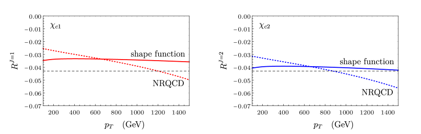
Figure 4: Dimensionless singlet to octet ratios $R^{J}$ for $J=1$ and $2$ from the shape function (solid lines) and NRQCD factorization (dotted lines) formalisms for production of $\chi_{c1}$ (left) and $\chi_{c2}$ (right) at central rapidity from $pp$ collisions at $\sqrt{s}=13$ TeV. The $\chi_{cJ}$ cross sections turn negative if the $R^{J}$ go below the matrix element ratio $-m^{2}\langle{\cal O}^{\chi_{c0}}(^{3}S_{1}^{[8]})\rangle/\langle{\cal O}^{\chi_{c0}}(^{3}P_{0}^{[1]})\rangle$, whose best-fit value $-0.043$ is shown as dashed black lines.

6.2 Nonperturbative corrections from shape functions

We now focus on the effect of nonperturbative corrections arising from the nonperturbative shape function that are neglected in usual applications of NRQCD factorization. That is, we make use of eq. (65) to compute the additional nonperturbative contribution coming from the deviation of the nonperturbative shape function from its asymptotic form. Because first-principles determination of the color-octet shape functions have not yet been done, this requires the use of model functions for the nonperturbative shape function. However, as we have argued previously, the normalization condition (49) and the requirement that the nonperturbative shape function must coincide with the asymptotic form at large $l_{+}$ severely constrain the model dependence. Additionally, the pNRQCD results for the shape functions imply that the $l_{+}$ dependence of the shape functions must be same for any $P$-wave heavy quarkonia, independently of radial excitation or heavy quark flavor; this lets us use a single model function for all shape functions for production of any $P$-wave heavy quarkonium state.

We first attempt a crude estimate of the size of the nonperturbative corrections at large transverse momentum $p_{T}$. We note that the factor ${\cal S}_{{}^{3}S_{1}^{[8]}}^{\chi_{Q0}}(l_{+})\big{|}_{\rm NP}-{\cal S}_{{}^{3}S_{1}^{[8]}}^{\chi_{Q0}}(l_{+})\big{|}_{\rm asy}$ in eq. (65) diminishes as $l_{+}$ increases, as the nonperturbative shape function must coincide with its asymptotic form when $l_{+}$ is in the perturbative regime. In the opposite case, when $l_{+}$ approaches zero, ${\cal S}_{{}^{3}S_{1}^{[8]}}^{\chi_{Q0}}(l_{+})\big{|}_{\rm asy}$ diverges like $1/l_{+}$, while the nonperturbative shape function must either be finite or at least diverge slower than $1/l_{+}$ in order to ensure the IR finiteness of its normalization. This implies that at very small values of $l_{+}$, we can approximate ${\cal S}_{{}^{3}S_{1}^{[8]}}^{\chi_{Q0}}(l_{+})\big{|}_{\rm NP}-{\cal S}_{{}^{3}S_{1}^{[8]}}^{\chi_{Q0}}(l_{+})\big{|}_{\rm asy}$ by $-{\cal S}_{{}^{3}S_{1}^{[8]}}^{\chi_{Q0}}(l_{+})\big{|}_{\rm asy}$. Hence, the additional nonperturbative contribution in eq. (65) can be estimated as

$$\sigma[\chi_{QJ}(P)]_{\rm NP} = (2J+1)\int_{0}^{\infty}dl_{+}\left(c_{{}^{3}S_{1}^{[8]}}(P+l)-c_{{}^{3}S_{1}^{[8]}}(P)\theta(l_{+}^{\rm max}-l_{+})\right)$$

$$\hskip 86.11084pt\times\Big{(}{\cal S}_{{}^{3}S_{1}^{[8]}}^{\chi_{Q0}}(l_{+})\Big{|}_{\rm NP}-{\cal S}_{{}^{3}S_{1}^{[8]}}^{\chi_{Q0}}(l_{+})\Big{|}_{\rm asy}\Big{)}$$

$$\approx -\int_{0}^{l_{+}^{\rm NP}}dl_{+}\left(c_{{}^{3}S_{1}^{[8]}}(P+l)-c_{{}^{3}S_{1}^{[8]}}(P)\right){\cal S}_{{}^{3}S_{1}^{[8]}}^{\chi_{Q0}}(l_{+})\Big{|}_{\rm asy},$$ (82)

where $l_{+}^{\rm NP}$ is chosen so that ${\cal S}_{{}^{3}S_{1}^{[8]}}^{\chi_{Q0}}(l_{+})\big{|}_{\rm NP}-{\cal S}_{{}^{3}S_{1}^{[8]}}^{\chi_{Q0}}(l_{+})\big{|}_{\rm asy}\approx-{\cal S}_{{}^{3}S_{1}^{[8]}}^{\chi_{Q0}}(l_{+})\big{|}_{\rm asy}$ for $l_{+}\lesssim l_{+}^{\rm NP}$. Note that $\sigma[\chi_{QJ}(P)]_{\rm NP}$ is positive in this case, because usually $c_{{}^{3}S_{1}^{[8]}}(P+l)<c_{{}^{3}S_{1}^{[8]}}(P)$ as the extra momentum $l$ reduces the available phase space. In the case of inclusive production at large $p_{T}$, the $p_{T}$-differential color-octet cross sections fall off like $1/p_{T}^{n}$, with $n\approx 4$. This, and the fact that at large $p_{T}$ the color-octet $Q\bar{Q}$ is produced predominantly near threshold through gluon fragmentation leads to the following approximation for the $l_{+}$ dependence of the short-distance coefficient:

$$c_{{}^{3}S_{1}^{[8]}}(P+l)\approx c_{{}^{3}S_{1}^{[8]}}(P)\left(\frac{P_{+}}{P_{+}+l_{+}}\right)^{n}\approx c_{{}^{3}S_{1}^{[8]}}(P)\left(1-\frac{nl_{+}}{P_{+}}\right),$$ (83)

where in the last equality we expanded in powers of $l_{+}$ to linear order compared to $P_{+}$, because $l_{+}^{\rm NP}$ is much smaller than $P_{+}$. By using this result, we can make the following estimate

$$\sigma[\chi_{QJ}(P)]_{\rm NP} \approx (2J+1)c_{{}^{3}S_{1}^{[8]}}(P)\int_{0}^{l_{+}^{\rm NP}}dl_{+}\frac{nl_{+}}{P_{+}}\times\frac{4\alpha_{s}C_{F}}{3N_{c}\pi m^{2}l_{+}}\langle{\cal O}^{\chi_{Q0}}(^{3}P_{0}^{[1]})\rangle$$ (84)

$$= (2J+1)c_{{}^{3}S_{1}^{[8]}}(P)\frac{nl_{+}^{\rm NP}}{P_{+}}\times\frac{4\alpha_{s}C_{F}}{3N_{c}\pi m^{2}}\langle{\cal O}^{\chi_{Q0}}(^{3}P_{0}^{[1]})\rangle.$$

Note that the boost-invariant ratio $l_{+}^{\rm NP}/P_{+}$ must be much smaller than $1/2$, because $P_{+}^{*}=2m$ gives $l_{+}^{\rm max}/P_{+}=e^{-1/6}/2$ when $\Lambda=m$. If we set $l_{+}^{\rm NP}/P_{+}=\lambda/2$, with $\lambda\ll 1$, the additional nonperturbative contribution to the cross section from the $P$-wave quarkonium cross section is estimated to be

$$\sigma[\chi_{QJ}(P)]_{\rm NP}\approx(2J+1)c_{{}^{3}S_{1}^{[8]}}(P)\frac{4\alpha_{s}C_{F}}{3N_{c}\pi m^{2}}\langle{\cal O}^{\chi_{Q0}}(^{3}P_{0}^{[1]})\rangle\times\frac{n\lambda}{2}.$$ (85)

Compare this with the color-octet contribution to the cross section in the NRQCD factorization formalism given by

$$\sigma[\chi_{QJ}(P)]_{\rm octet}=(2J+1)c_{{}^{3}S_{1}^{[8]}}(P)\frac{{\cal E}_{11}}{3N_{c}^{2}m^{2}}\langle{\cal O}^{\chi_{Q0}}(^{3}P_{0}^{[1]})\rangle,$$ (86)

where we used the pNRQCD result for the color-octet matrix element to write the cross section in terms of the color-singlet matrix element and the universal quantity ${\cal E}_{11}$. In the case of $\chi_{cJ}$, best-fit values of $P$-wave quarkonium matrix elements give ${\cal E}_{11}=1.17$ at scale $\Lambda=1.5$ GeV Ma:2010vd ; Brambilla:2021abf . By setting $\alpha_{s}=0.25$ at the scale of the charmonium mass, $\lambda=0.5$, and $n=4$, we find that $\sigma[\chi_{QJ}(P)]_{\rm NP}$ is of roughly the same order of magnitude as $\sigma[\chi_{QJ}(P)]_{\rm octet}$ in the case of charmonium production. In the case of bottomonium, $\sigma[\chi_{QJ}(P)]_{\rm NP}$ is smaller than $\sigma[\chi_{QJ}(P)]_{\rm octet}$, because ${\cal E}_{11}$ becomes larger at the scale of the bottom quark mass.

Even though the additional nonperturbative effects from nonperturbative shape functions estimated in eq. (85) can be as large as order one compared to NRQCD calculations of the cross section, this by itself is inconsequential in large-$p_{T}$ quarkonium production phenomenology, because the additional contributions do not alter the $p_{T}$ dependence of the cross section and only brings in changes in the overall normalization. That is, the additional nonperturbative contributions can be absorbed into a redefinition of the color-octet matrix element. Because in phenomenological analyses the color-octet matrix elements are obtained from measured cross sections, and not computed from first principles, this redefinition does not affect the large-$p_{T}$ phenomenology in any way. It should be noted, however, that this estimate is valid only for the large-$p_{T}$ asymptotic behavior of the cross section. At smaller values of $p_{T}$, the shapes of the color-octet cross sections change, which would invalidate the assumptions that lead us to the estimate in eq. (85). Hence, at smaller values of $p_{T}$, the additional nonperturbative contributions may change the $p_{T}$ shapes of the cross section significantly. In order to investigate these effects quantitatively, we need to compute $\sigma[\chi_{QJ}(P)]_{\rm NP}$ explicitly with model shape functions.

Before we go on with the computation of the cross section, we discuss another nonperturbative effect associated with the heavy quarkonium mass that can be incorporated in the shape function formalism. As have been discussed in ref. Beneke:1997qw , the shape function formalism allows matching the $Q\bar{Q}$ phase space with the physical one involving the heavy quarkonium mass. In NRQCD factorization, the invariant mass of the $Q\bar{Q}$ produced in the short-distance process can be different from the heavy quarkonium mass by order $mv$, due to the fact that the $Q\bar{Q}$ can emit order-$mv$ gluons before evolving into a quarkonium. In the shape function formalism, the kinematics of the emission of order-$mv$ gluons is explicitly taken into account by the $l_{+}$ dependences in the shape functions and the corresponding short-distance coefficients. Hence, as have been suggested in ref. Beneke:1997qw , in the calculation of the short-distance coefficients $s_{N}(P+l)$ and $s_{N}(P)$, the $Q\bar{Q}$ mass $m_{Q\bar{Q}}=\sqrt{P^{2}}$ can be chosen to be the heavy quarkonium mass, instead of $m_{Q\bar{Q}}=2m$. In principle, in the nonrelativistic power counting the difference between $2m$ and the heavy quarkonium mass is of order $mv^{2}$. Because the shape functions describe the emission of order-$mv$ gluons, and not necessarily order-$mv^{2}$ effects, the order-$mv^{2}$ effects can be consistently neglected from the short-distance coefficients by setting $m_{Q\bar{Q}}=2m$ in the same way as done in NRQCD. However, because of the renormalon ambiguity in the heavy quark pole mass, the difference between the heavy quarkonium mass and $2m$ can exceed $mv^{2}$ and become numerically significant depending on the choice of the pole mass $m$. Setting $m_{Q\bar{Q}}$ to be the quarkonium mass avoids this issue and ensures that the $Q\bar{Q}$ phase space matches the physical one within order $mv^{2}$.

We now compute the $\chi_{c}$ and $\chi_{b}$ cross sections in NRQCD and shape function formalisms. Since we are interested in the nonperturbative effects from the shape function formalism at values of $p_{T}$ lower than the fragmentation regime, we compute the cross sections for the LHCb kinematics from 7 TeV $pp$ collisions at the LHC, where data for $P$-wave quarkonium production rates relative to $1S$ quarkonium production rates are available for $p_{T}\geq 2$ GeV for $\chi_{c}$ LHCb:2012af and $p_{T}\geq 6$ GeV for $\chi_{b}$ LHCb:2014ngh , which go below the quarkonium masses. The available $p_{T}$ ranges are, however, above the heavy quark pole masses which we set to be $m=1.5$ GeV for charm and $m=4.75$ GeV for bottom. The cross sections are computed in NRQCD and shape function formalisms as

$$\frac{d\sigma[\chi_{QJ}]}{dp_{T}}\Big{|}_{\rm NRQCD} = (2J+1)\bigg{(}\frac{d\sigma[Q\bar{Q}(^{3}P_{J}^{[1]})]}{dp_{T}}\langle{\cal O}^{\chi_{Q0}}(^{3}P_{0}^{[1]})\rangle+\frac{d\sigma[Q\bar{Q}(^{3}S_{1}^{[8]})]}{dp_{T}}\langle{\cal O}^{\chi_{Q0}}(^{3}S_{1}^{[8]})\rangle\bigg{)},$$

$$\frac{d\sigma[\chi_{QJ}]}{dp_{T}}\Big{|}_{\rm shape} = (2J+1)\bigg{(}\frac{d\sigma[Q\bar{Q}(^{3}P_{J}^{[1]})]}{dp_{T}}\langle{\cal O}^{\chi_{Q0}}(^{3}P_{0}^{[1]})\rangle+\frac{d\sigma[Q\bar{Q}(^{3}S_{1}^{[8]})]}{dp_{T}}\langle{\cal O}^{\chi_{Q0}}(^{3}S_{1}^{[8]})\rangle\bigg{)}$$ (87b)

$$+\frac{d\sigma[\chi_{QJ}]}{dp_{T}}\bigg{|}_{\rm NP},$$

where

$$\frac{d\sigma[\chi_{QJ}]}{dp_{T}}\bigg{|}_{\rm NP} = (2J+1)\int_{0}^{\infty}dl_{+}\left(\frac{d\sigma[Q\bar{Q}(^{3}S_{1}^{[8]})]}{dp_{T}}\Big{|}_{P\to P+l}-\frac{d\sigma[Q\bar{Q}(^{3}S_{1}^{[8]})]}{dp_{T}}\theta(l_{+}^{\rm max}-l_{+})\right)$$ (88)

$$\hskip 86.11084pt\times\Big{(}{\cal S}_{{}^{3}S_{1}^{[8]}}^{\chi_{Q0}}(l_{+})\Big{|}_{\rm NP}-{\cal S}_{{}^{3}S_{1}^{[8]}}^{\chi_{Q0}}(l_{+})\Big{|}_{\rm asy}\Big{)}.$$

We compute the NRQCD short-distance coefficients at NLO in $\alpha_{s}$ numerically by using the FDCHQHP package Wan:2014vka with CTEQ6M parton distribution functions Pumplin:2002vw . Note that $d\sigma[\chi_{QJ}]/dp_{T}|_{\rm shape}$ involve the same short-distance coefficients as NRQCD, but in this case we compute them with the $Q\bar{Q}$ mass set to be the physical $\chi_{QJ}$ mass, while in the NRQCD cross section the $Q\bar{Q}$ mass is $2m$, as is usually done in phenomenological studies. We compute the short-distance coefficients that enter the nonperturbative correction term $d\sigma[\chi_{QJ}]/dp_{T}|_{\rm NP}$ at leading order in $\alpha_{s}$ from the known parton cross sections $d\hat{\sigma}[ij\to Q\bar{Q}(^{3}S_{1}^{[8]})+X]/d\hat{t}$ where $i,j=g$, $q$, and $\bar{q}$, and $\hat{t}$ is a partonic Mandelstam variable. For the term involving $\theta(l_{+}^{\rm max}-l_{+})$, we can compute the $d\sigma[Q\bar{Q}(^{3}S_{1}^{[8]})]/dp_{T}$ at tree level as

$$\frac{d\sigma[Q\bar{Q}(^{3}S_{1}^{[8]})]}{dp_{T}}=\sum_{i,j=g,q,\bar{q}}\int dydy^{\prime}\left(2p_{T}x_{1}x_{2}\right)f_{i/p}(x_{1})f_{j/p}(x_{2})\frac{d\hat{\sigma}[ij\to Q\bar{Q}(^{3}S_{1}^{[8]})+X]}{d\hat{t}},$$ (89)

where $f_{i/p}(x)$ is the parton distribution function for finding a parton $i$ with momentum fraction $x$ in a proton, $y$ is the rapidity of the $Q\bar{Q}$, and $y^{\prime}$ is the rapidity of the recoil $X$. The factor $2p_{T}x_{1}x_{2}$ is the Jacobian arising from the change of integration variables from $x_{1}$, $x_{2}$, and $\hat{t}$ to $p_{T}$, $y$, and $y^{\prime}$. The parton cross sections $d\hat{\sigma}[ij\to Q\bar{Q}(^{3}S_{1}^{[8]})+X]/d\hat{t}$ are available as functions of the partonic Mandelstam variables $\hat{s}$, $\hat{u}$, and $\hat{t}$, which can be written in terms of $s$, $p_{T}$, $y$, $y^{\prime}$, and $P^{2}=m_{Q\bar{Q}}^{2}$ as

$$\hat{s} = x_{1}x_{2}s,$$ (90a)

$$\hat{t} = m_{Q\bar{Q}}^{2}-x_{1}\sqrt{s}m_{T}e^{-y},$$ (90b)

$$\hat{u} = m_{Q\bar{Q}}^{2}-\hat{s}-\hat{t},$$ (90c)

where $m_{T}=\sqrt{m_{Q\bar{Q}}^{2}+p_{T}^{2}}$, $x_{1}=(m_{T}e^{y}+p_{T}e^{y^{\prime}})/\sqrt{s}$, and $x_{2}=(m_{T}e^{-y}+p_{T}e^{-y^{\prime}})/\sqrt{s}$. Analytical expressions for the tree-level $2\to 2$ parton cross sections for $gg$, $gq$, and $q\bar{q}$ initial states can be found in ref. Cho:1995vh . The calculation of $d\sigma[Q\bar{Q}(^{3}S_{1}^{[8]})]/dp_{T}\big{|}_{P\to P+l}$ is carried out in a similar way, except now the partonic Mandelstam variables are given by

$$\hat{s} = x_{1}x_{2}s,$$ (91a)

$$\hat{t} = m_{Q\bar{Q}}^{2}+(m_{T}-p_{T})l_{T}-x_{1}\sqrt{s}(m_{T}+l_{T})e^{-y},$$ (91b)

$$\hat{u} = m_{Q\bar{Q}}^{2}+(m_{T}-p_{T})l_{T}-\hat{s}-\hat{t},$$ (91c)

where $x_{1}=[(m_{T}+l_{T})e^{y}+(p_{T}+l_{T})e^{y^{\prime}}]/\sqrt{s}$, $x_{2}=[(m_{T}+l_{T})e^{-y}+(p_{T}+l_{T})e^{-y^{\prime}}]/\sqrt{s}$, and $l_{T}$ is the transverse component of $l$. Note that there is some ambiguity in choosing the direction of the momentum $l$, because boosts along the beam direction will change the directions of $\bm{P}$ and $\bm{l}$ differently. We choose the directions of $\bm{l}$ and $\bm{P}$ to coincide in the frame where $|\bm{P}|=p_{T}$ and $|\bm{l}|=l_{T}$. In this frame, $l_{+}=2|\bm{l}|=2l_{T}$, and the boost to this frame from the rest frame of the $\chi_{Q}$ is given by $l_{+}=l_{+}^{*}\times(m_{T}+p_{T})/m_{Q\bar{Q}}$. The short-distance coefficient $d\sigma[Q\bar{Q}(^{3}S_{1}^{[8]})]/dp_{T}\big{|}_{P\to P+l}$ can be computed in a similar form as eq. (89), where now the $l$-dependent partonic Mandelstam variables are given in eqs. (91), and the Jacobian now takes a more complicated $l$-dependent form.

In order to compute $d\sigma[\chi_{QJ}]/dp_{T}\big{|}_{\rm NP}$, the parton cross sections $d\hat{\sigma}/d\hat{t}$ for the color-octet channel must be known as functions of the partonic Mandelstam variables. The analytical expressions for $gg$, $gq$, and $q\bar{q}$ initial states are available at tree level (order $\alpha_{s}^{3}$) in ref. Cho:1995vh . At NLO (order $\alpha_{s}^{4}$), publicly available results are given only as $p_{T}$-differential cross sections convolved with parton distribution functions and integrated over rapidity ranges, so that they cannot be used directly in eq. (88) to compute $d\sigma[\chi_{QJ}]/dp_{T}\big{|}_{\rm NP}$. Fortunately, in the kinematical ranges that we are interested in this section, the effect of the NLO correction is small for the color-octet channel: as can be seen in ref. Ma:2010yw , the NLO $K$ factor for the ${}^{3}S_{1}^{[8]}$ channel is close to $1$ and is almost constant in $p_{T}$. Hence, we neglect the NLO corrections to $d\sigma[Q\bar{Q}(^{3}S_{1}^{[8]})]/dp_{T}$ when we compute the nonperturbative corrections $d\sigma[\chi_{QJ}]/dp_{T}\big{|}_{\rm NP}$, while we compute the short-distance coefficients at NLO accuracy everywhere else.

Now we need a model for the nonperturbative shape function. As we have stated earlier, the nonperturbative shape function ${\cal S}_{{}^{3}S_{1}^{[8]}}^{\chi_{Q0}}(l_{+})\big{|}_{\rm NP}$ must take the asymptotic form ${\cal S}_{{}^{3}S_{1}^{[8]}}^{\chi_{Q0}}(l_{+})\big{|}_{\rm asy}$ for $l_{+}\gtrsim l_{+}^{\rm max}$, and normalized by $\int_{0}^{l_{+}^{\rm max}}dl_{+}{\cal S}_{{}^{3}S_{1}^{[8]}}^{\chi_{Q0}}(l_{+})\big{|}_{\rm NP}=\langle{\cal O}^{\chi_{Q0}}(^{3}S_{1}^{[8]})\rangle^{\overline{\rm MS}}$. For the normalization integral to be IR finite, the nonperturbative shape function must either be finite, or at least diverge slower than $1/l_{+}$ as $l_{+}\to 0$. We consider the following model functions

$${\cal S}_{{}^{3}S_{1}^{[8]}}^{\chi_{Q0}}(l_{+})\big{|}_{\textrm{model 1}} = \frac{4\alpha_{s}C_{F}}{3N_{c}\pi m^{2}}\langle{\cal O}^{\chi_{Q0}}(^{3}P_{0}^{[1]})\rangle\frac{l_{+}}{l_{+}^{2}+a_{+}^{2}},$$ (92a)

$${\cal S}_{{}^{3}S_{1}^{[8]}}^{\chi_{Q0}}(l_{+})\big{|}_{\textrm{model 2}} = \frac{4\alpha_{s}C_{F}}{3N_{c}\pi m^{2}}\langle{\cal O}^{\chi_{Q0}}(^{3}P_{0}^{[1]})\rangle\frac{1}{(l_{+}^{2}+a_{+}^{2})^{1/2}},$$ (92b)

$${\cal S}_{{}^{3}S_{1}^{[8]}}^{\chi_{Q0}}(l_{+})\big{|}_{\textrm{model 3}} = \frac{4\alpha_{s}C_{F}}{3N_{c}\pi m^{2}}\langle{\cal O}^{\chi_{Q0}}(^{3}P_{0}^{[1]})\rangle\frac{1}{l_{+}}\theta(a_{+}-l_{+}),$$ (92c)

$${\cal S}_{{}^{3}S_{1}^{[8]}}^{\chi_{Q0}}(l_{+})\big{|}_{\textrm{model 4}} = \frac{4\alpha_{s}C_{F}}{3N_{c}\pi m^{2}}\langle{\cal O}^{\chi_{Q0}}(^{3}P_{0}^{[1]})\rangle\frac{1}{l_{+}[(a_{+}/l_{+})^{2}+1]^{\alpha/2}},\quad 0<\alpha<1.$$ (92d)

In model 1, the model shape function vanishes linearly as $l_{+}\to 0$, while in model 2 the model function becomes a finite constant. The model 3 shape function coincides the asymptotic form for $l_{+}>a_{+}$, while it vanishes for $l_{+}<a_{+}$. In model 4, the model function diverges as $l_{+}\to 0$ like $1/l_{+}^{1-\alpha}$, more slowly than the asymptotic form, to ensure the IR finiteness of the normalization integral. We use the value $\alpha=0.8$ so that the model function slowly diverges at $l_{+}=0$, and recovers the asymptotic form at large $l_{+}$. The model parameters $a_{+}$, which transforms under boosts like $l_{+}$, can be determined from the normalization condition. By using the value $\alpha_{s}=0.33$ at scale $1.5$ GeV, and the best-fit value for $\chi_{cJ}$ matrix elements giving $m^{2}\langle{\cal O}^{\chi_{c0}}(^{3}S_{1}^{[8]})\rangle/\langle{\cal O}^{\chi_{c0}}(^{3}P_{0}^{[1]})\rangle=0.043$ at $\Lambda=1.5$ GeV Ma:2010vd ; Brambilla:2021abf , we obtain the model parameters at the rest frame of the $\chi_{Q0}$ given by $a_{+}^{*}=0.74$, 1.7, 0.64, and 2.6 in units of GeV for models 1, 2, 3, and 4, respectively. The shapes in $l_{+}^{*}$ of theses model functions for fixed values of the model parameters are shown in fig. 5 compared to the asymptotic form.

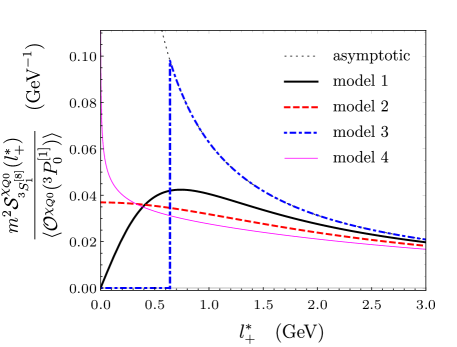
Figure 5: Shapes in $l_{+}^{*}$ of the model functions for the color-octet shape function ${\cal S}_{{}^{3}S_{1}^{[8]}}^{\chi_{Q0}}(l^{*}_{+})$ divided by $\langle{\cal O}^{\chi_{Q0}}(^{3}P_{0}^{[1]})\rangle/m^{2}$ for model 1 (black solid line), model 2 (red dashed line), model 3 (blue dot-dashed line), and model 4 (thin magenta line), compared to the asymptotic form (thin dotted line). The model parameter for each model is determined from the normalization eq. (49) and the NLO best-fit value $m^{2}\langle{\cal O}^{\chi_{c0}}(^{3}S_{1}^{[8]})\rangle/\langle{\cal O}^{\chi_{c0}}(^{3}P_{0}^{[1]})\rangle=0.043$ at $\Lambda=1.5$ GeV.

In order to investigate the model dependence of the cross section in the shape function formalism, we compute $d\sigma[\chi_{QJ}]/dp_{T}\big{|}_{\rm NP}$ from the four model shape functions. In order to assess the impact of the nonperturbative corrections, we compute the dimensionless ratios of the color-octet channel contributions in the NRQCD and shape function formalisms

$$r^{Q}_{\rm octet}=\frac{\displaystyle\frac{d\sigma[\chi_{QJ}]}{dp_{T}}\Big{|}_{\textrm{octet, shape}}}{\displaystyle\frac{d\sigma[\chi_{QJ}]}{dp_{T}}\Big{|}_{\textrm{octet, NRQCD}}},$$ (93)

where the numerator and denominator are defined by

$$\frac{d\sigma[\chi_{QJ}]}{dp_{T}}\Big{|}_{\textrm{octet, shape}} = (2J+1)\frac{d\sigma[Q\bar{Q}(^{3}S_{1}^{[8]})]}{dp_{T}}\langle{\cal O}^{\chi_{Q0}}(^{3}S_{1}^{[8]})\rangle+\frac{d\sigma[\chi_{QJ}]}{dp_{T}}\bigg{|}_{\rm NP}.$$ (94a)

$$\frac{d\sigma[\chi_{QJ}]}{dp_{T}}\Big{|}_{\textrm{octet, NRQCD}} = (2J+1)\frac{d\sigma[Q\bar{Q}(^{3}S_{1}^{[8]})]}{dp_{T}}\langle{\cal O}^{\chi_{Q0}}(^{3}S_{1}^{[8]})\rangle,$$ (94b)

Since we are interested in the behavior of $d\sigma[\chi_{QJ}]/dp_{T}$ compared to the color-octet channel contribution in the usual NRQCD factorization formalism, we compute the short-distance coefficients $d\sigma[Q\bar{Q}(^{3}S_{1}^{[8]})/dp_{T}$ at tree level (order $\alpha_{s}^{3}$) for the calculation of $r^{Q}_{\rm octet}$ (we will use the full NLO results in the calculation of cross sections for comparison with measurements). As we have stated earlier, we set the $Q\bar{Q}$ mass to be $2m$ for the cross section in NRQCD, while we set it to be the quarkonium mass in the shape function formalism. The ratios depend on the ratio of NRQCD matrix elements $m^{2}\langle{\cal O}^{\chi_{Q0}}(^{3}S_{1}^{[8]})\rangle/\langle{\cal O}^{\chi_{Q0}}(^{3}P_{0}^{[1]})\rangle$. For charmonium we set it to be the best-fit value 0.043 at $\Lambda=1.5$ GeV. For bottomonium, we compute the ratio for $\chi_{b0}$ at scale $4.75$ GeV by using the universality of the gluonic quantity ${\cal E}_{11}$ and its evolution equation Brambilla:2021abf . That is,

$$\frac{m^{2}\langle{\cal O}^{\chi_{b0}}(^{3}S_{1}^{[8]})\rangle(\Lambda=4.75\textrm{~{}GeV})}{\langle{\cal O}^{\chi_{b0}}(^{3}P_{0}^{[1]})\rangle} = \frac{m^{2}\langle{\cal O}^{\chi_{c0}}(^{3}S_{1}^{[8]})\rangle(\Lambda=1.5\textrm{~{}GeV})}{\langle{\cal O}^{\chi_{c0}}(^{3}P_{0}^{[1]})\rangle}$$ (95)

$$+\frac{1}{(d-1)N_{c}^{2}}\frac{24C_{F}}{\beta_{0}}\log\frac{\alpha_{s}(1.5\textrm{~{}GeV})}{\alpha_{s}(4.75\textrm{~{}GeV})}.$$

where the left-hand side equals ${\cal E}_{11}/[(d-1)N_{c}^{2}]$ at scale 4.75 GeV, and the last line comes from the evolution of this quantity from scale 1.5 GeV to 4.75 GeV. Numerically, we obtain similar numbers if we use the model shape functions and integrate over $l_{+}^{*}$ up to $l_{+}^{*\rm max}=4.75\times e^{-1/6}$ GeV. This result is compatible with the NLO fit results for $\chi_{b}$ matrix elements Han:2014kxa , and has been used successfully in phenomenological analyses of $\chi_{b}$ cross sections based on the pNRQCD formalism Brambilla:2021abf .

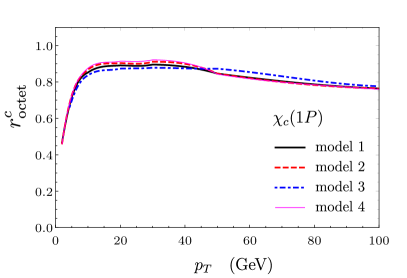
Figure 6: The ratio of the color-octet channel contributions in the shape function and NRQCD formalisms $r^{c}_{\rm octet}$ for production of $\chi_{c}$ computed from model shape functions with model 1 (black solid line), model 2 (red dashed line), model 3 (blue dot-dashed line), and model 4 (thin magenta line).

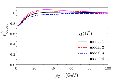
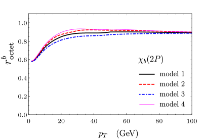
Figure 7: The ratio of the color-octet channel contributions in the shape function and NRQCD formalisms $r^{b}_{\rm octet}$ for production of $\chi_{b}(1P)$ (left) and $\chi_{b}(2P)$ (right) computed from model shape functions with model 1 (black solid line), model 2 (red dashed line), model 3 (blue dot-dashed line), and model 4 (thin magenta line).

The results for $r^{c}_{\rm octet}$ for the model shape functions are shown in fig 6. The ratio is below 1, even though $d\sigma[\chi_{QJ}]/dp_{T}|_{\rm NP}$ is positive; this happens because the short-distance coefficient $d\sigma[Q\bar{Q}(^{3}S_{1}^{[8]})]/dp_{T}$ is smaller for the shape function formalism due to the use of a larger value of the $Q\bar{Q}$ mass, which reduces the overall normalization of the short-distance coefficient through the nonrelativistic normalization of the $Q\bar{Q}$ state. The model dependence is small, amounting to less than $\pm 0.022$. Regardless of the model chosen to compute $d\sigma[\chi_{QJ}]/dp_{T}|_{\rm NP}$, the ratio $r^{c}_{\rm octet}$ is nearly flat for values of $p_{T}$ above about 20 GeV, consistently with the estimate we made in the beginning of this section. At lower values of $p_{T}$, the ratio changes slope and steadily decreases as $p_{T}$ drops below from about 10 GeV. This is a combined effect of the reduction of the relative size of $d\sigma[\chi_{QJ}]/dp_{T}|_{\rm NP}$ compared to $d\sigma[\chi_{QJ}]/dp_{T}|_{\textrm{octet, NRQCD}}$, and the reduction of $d\sigma[Q\bar{Q}(^{3}S_{1}^{[8]})]/dp_{T}$ at $m_{Q\bar{Q}}=m_{\chi_{c}}$ compared to the $m_{Q\bar{Q}}=2m$ case. This behavior is similar for $r^{b}_{\rm octet}$ for $1P$ and $2P$ states, as shown in fig. 7. The deviation of the ratio $r^{b}_{\rm octet}$ from one is less severe than the charmonium case. In the case of $r^{b}_{\rm octet}$, the model dependence is less than about $\pm 0.049$ for both $\chi_{b}(1P)$ and $\chi_{b}(2P)$. The values for $r^{b}_{\rm octet}$ are smaller for $\chi_{b}(2P)$ compared to $\chi_{b}(1P)$ at similar values of $p_{T}$, because the $2P$ state is heavier than the $1P$ state. Because in all cases model dependences are smaller than the usual estimates of theoretical uncertainties, we neglect the model dependence and compute $d\sigma[\chi_{QJ}]/dp_{T}|_{\rm NP}$ using shape function model 1, which gives results that are close to the average of all models considered here. Model 1 seems to be a reasonable choice, since if we were to interpret the nonlocal gluonic operator vacuum expectation value ${\cal E}\!\!\!/_{11}(l_{+})$ as the probability for a gluon with momentum $l$ to propagate to spacetime infinity, we would expect the probability to vanish as $l\to 0$ due to confinement.

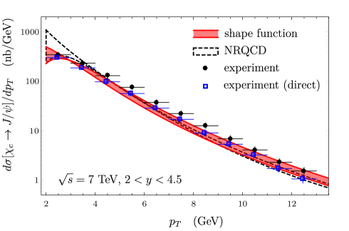
Figure 8: Production rate of $J/\psi$ from $\chi_{c}$ decays in $pp$ collisions at $\sqrt{s}=7$ TeV in the rapidity range $2<y<4.5$ computed from the shape function (red band) and NRQCD (dashed outlined band) formalisms as functions of the $J/\psi$ transverse momentum. Experimental values (black filled circles) are obtained from the prompt $J/\psi$ cross section and the feeddown fraction measurements from LHCb LHCb:2011zfl ; LHCb:2012af . The “direct” experimental values (blue open squares) are obtained by subtracting the contribution from the cascade decay $\psi(2S)\to\chi_{c}+X$ followed by $\chi_{c}\to J/\psi+\gamma$, which is computed from the prompt $\psi(2S)$ cross section measurements from LHCb LHCb:2012geo and the measured branching fractions in ref. ParticleDataGroup:2022pth .

We now compute the cross sections for $\chi_{c}$ at $pp$ collisions at center-of-mass energy $\sqrt{s}=7$ TeV with rapidity cut $2<y<4.5$. For this we need to determine the values of NRQCD matrix elements. We compute the color-singlet matrix element from the well-known result $\langle{\cal O}^{\chi_{c0}}(^{3}P_{0}^{[1]})\rangle=\frac{3N_{c}}{2\pi}|R^{\prime}(0)|^{2}$, which is also consistent with pNRQCD calculations of the color-singlet matrix element, and use the determination $|R^{\prime}(0)|^{2}=0.057$ GeV⁵ obtained in ref. Brambilla:2021abf from two-photon decay rates of $\chi_{c0}$ and $\chi_{c2}$. For the color-octet matrix element, we use the NLO best-fit value $m^{2}\langle{\cal O}^{\chi_{Q0}}(^{3}S_{1}^{[8]})\rangle/\langle{\cal O}^{\chi_{Q0}}(^{3}P_{0}^{[1]})\rangle=0.043$ at $\Lambda=1.5$ GeV Brambilla:2021abf , as we have done for the determination of the parameters of our model shape functions. As we have stated earlier, we compute the NLO short-distance coefficients for the color-singlet and color-octet channels using the FDCHQHP Fortran package Wan:2014vka with CTEQ6M parton distribution functions Pumplin:2002vw . We set the scales for $\alpha_{s}$ and the parton distributions functions to be $m_{T}=\sqrt{p_{T}^{2}+m_{Q\bar{Q}}^{2}}$, and vary them simultaneously between $\tfrac{1}{2}m_{T}$ and $2m_{T}$, as have been done in many phenomenological studies of quarkonium production. To match what have been measured in experiments, we compute the combined cross sections

$$\frac{d\sigma[\chi_{c}\to J/\psi]}{dp_{T}}=\sum_{J=1,2}B_{\chi_{cJ}\to J/\psi+\gamma}\frac{d\sigma[\chi_{cJ}]}{dp_{T}},$$ (96)

as functions of $J/\psi$ transverse momentum $p_{T}^{J/\psi}$. We estimate $p_{T}^{J/\psi}$ by using the formula

$$p_{T}^{J/\psi}=\frac{m_{J/\psi}}{m_{\chi_{c}}}p_{T}^{\chi_{c}},$$ (97)

which follows from the fact that the processes $\chi_{cJ}\to J/\psi+\gamma$ for $J=1$ and 2 are mainly E1 transitions. We take the $\chi_{cJ}\to J/\psi+\gamma$ branching fractions from ref. ParticleDataGroup:2022pth . We neglect the contribution from $\chi_{c0}$, because the branching fraction $B_{\chi_{c0}\to J/\psi+\gamma}$ is very small. The results for $d\sigma[\chi_{c}\to J/\psi]/dp_{T}$ from NRQCD and the shape function formalisms are shown in fig. 8, compared to experimental values obtained from LHCb measurements. The experimental values for absolute cross sections have been obtained from the measurements of the ratio of $\chi_{c}$ to $J/\psi$ production rates in ref. LHCb:2012af and the measured prompt $J/\psi$ production rates in ref. LHCb:2011zfl . Note that the prompt cross section measurements in ref. LHCb:2011zfl include feeddowns from decays of $\psi(2S)$, while our calculation does not; to facilitate a better comparison, we also show experimental values for feeddown-subtracted $\chi_{c}$ cross sections, which we obtain from the measured $\psi(2S)$ cross sections in ref. LHCb:2012geo and the branching fractions $B_{\psi(2S)\to\chi_{cJ}+X}$ for $J=1$ and 2 from ref. ParticleDataGroup:2022pth . The difference between results from the NRQCD and the shape function formalisms are rather small and are within the theoretical uncertainties, except when $p_{T}\approx m_{\chi_{c}}$: for $p_{T}$ around 3–5 GeV, the cross section in the shape function formalism is smaller than the result from the NRQCD formalism, and agrees better with the feeddown-subtracted experimental values. While this difference slightly improves agreement with experiment, it only amounts to about 30%, which is the nominal size of corrections suppressed by $v^{2}$ that are neglected in both NRQCD and shape function formalisms.

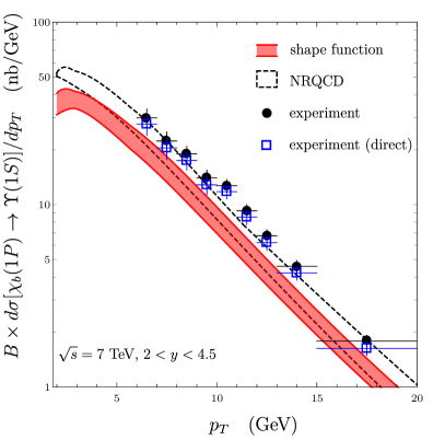
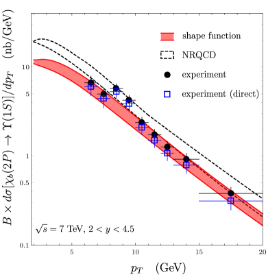
Figure 9: Production rate of $\Upsilon(1S)$ from $\chi_{b}(1P)$ (left) and $\chi_{b}(2P)$ (right) decays times the branching fraction $B\equiv B_{\Upsilon(1S)\to\mu^{+}\mu^{-}}$ in $pp$ collisions at $\sqrt{s}=7$ TeV in the rapidity range $2<y<4.5$ computed from the shape function (red band) and NRQCD (dashed outlined band) formalisms as functions of the $\Upsilon$ transverse momentum. Experimental values (black filled circles) are obtained from the inclusive $\Upsilon$ cross section and the feeddown fraction measurements from LHCb LHCb:2014ngh ; LHCb:2015log . The “direct” experimental values (blue open squares) are obtained by subtracting the cascade decay contributions from $\Upsilon(2S)\to\chi_{b}(1P)+X$, $\Upsilon(3S)\to\chi_{b}(1P)+X$, and $\Upsilon(3S)\to\chi_{b}(2P)+X$, which are computed from the inclusive $\Upsilon(2S)$ and $\Upsilon(3S)$ cross section measurements from LHCb LHCb:2015log and measured branching fractions in ref. ParticleDataGroup:2022pth .

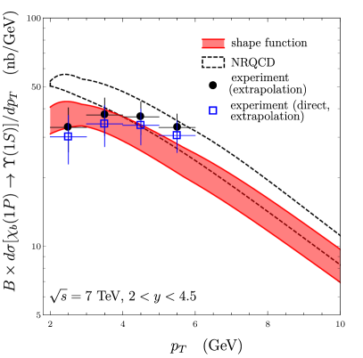
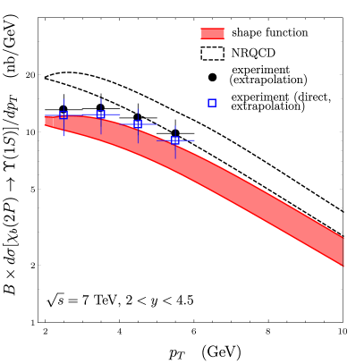
Figure 10: Production rate of $\Upsilon(1S)$ from $\chi_{b}(1P)$ (left) and $\chi_{b}(2P)$ (right) decays times the branching fraction $B\equiv B_{\Upsilon(1S)\to\mu^{+}\mu^{-}}$ in $pp$ collisions at $\sqrt{s}=7$ TeV in the rapidity range $2<y<4.5$ computed from the shape function (red band) and NRQCD (dashed outlined band) formalisms as functions of the $\Upsilon$ transverse momentum. Experimental values (black filled circles) for $p_{T}\leq 6$ GeV are obtained by using the measured inclusive $\Upsilon$ cross section in ref. LHCb:2015log and extrapolating the feeddown fraction measurements from LHCb LHCb:2014ngh to smaller values of $p_{T}$. The “direct” experimental values (blue open squares) are obtained by subtracting the cascade decay contributions from $\Upsilon(2S)\to\chi_{b}(1P)+X$, $\Upsilon(3S)\to\chi_{b}(1P)+X$, and $\Upsilon(3S)\to\chi_{b}(2P)+X$, which are computed from the inclusive $\Upsilon(2S)$ and $\Upsilon(3S)$ cross section measurements from LHCb LHCb:2015log and measured branching fractions in ref. ParticleDataGroup:2022pth .

We can repeat the same calculation for bottomonium: we compute cross sections for $\chi_{b}(1P)$ and $\chi_{b}(2P)$ for LHCb kinematics at $\sqrt{s}=7$ TeV and $2<y<4.5$. Similarly to the case of $\chi_{c}$ we need values for the NRQCD matrix elements. For the color-singlet matrix elements we again use the relation $\langle{\cal O}^{\chi_{b0}}(^{3}P_{0}^{[1]})\rangle=\frac{3N_{c}}{2\pi}|R^{\prime}(0)|^{2}$, with $|R^{\prime}(0)|^{2}=1.47$ GeV⁵ for $1P$ and $|R^{\prime}(0)|^{2}=1.74$ GeV⁵ for $2P$ states, which are averages of potential-model calculations considered in ref. Brambilla:2020xod . For the color-octet matrix element, we use the evolution equation in eq. (95) and the best-fit value for the matrix element ratio for $\chi_{c}$ to determine $\langle{\cal O}^{\chi_{b0}}(^{3}S_{1}^{[8]})\rangle$ at scale $\Lambda=4.75$ GeV. On the experimental side, LHCb measurements are available for the feeddown fractions in ref. LHCb:2014ngh for $\Upsilon(nS)$ from $\chi_{b}(n^{\prime}P)$ decays for $n$ and $n^{\prime}$ between 1 and 3 with $n^{\prime}\geq n$, and the absolute cross sections for $\Upsilon(nS)$ as functions of $p_{T}$ of $\Upsilon$ in ref. LHCb:2015log . We use the measured values for $\Upsilon(1S)$ cross sections and the feeddown fractions to obtain the experimental values for $\chi_{bJ}(n^{\prime}P)$ cross sections times branching fraction into $\Upsilon(1S)$, summed over $J$. To compare with the experimental values, we compute

$$\frac{B\times d\sigma[\chi_{b}(n^{\prime}P)\to\Upsilon(1P)]}{dp_{T}}=B\times\sum_{J=1,2}B_{\chi_{bJ}(n^{\prime}P)\to\Upsilon(1P)+\gamma}\frac{d\sigma[\chi_{bJ}(n^{\prime}P)]}{dp_{T}},$$ (98)

where $B\equiv B_{\Upsilon(1S)\to\mu^{+}\mu^{-}}$, as functions of $\Upsilon$ transverse momentum $p_{T}^{\Upsilon}$. We compute $p_{T}^{\Upsilon}$ by using

$$p_{T}^{\Upsilon}=\frac{m_{\Upsilon}}{m_{\chi_{b}(n^{\prime}P)}}p_{T}^{\chi_{b}(n^{\prime}P)}.$$ (99)

We take the measured branching fractions from ref. ParticleDataGroup:2022pth . Similarly to the charmonium case, we neglect the contribution from $\chi_{b0}$ on the account that its branching fraction into $\Upsilon$ is small. The results for $d\sigma[\chi_{b}(n^{\prime}P)\to\Upsilon(1P)]/dp_{T}$ from NRQCD and shape function formalisms are shown in fig. 9, compared to experimental values. As we have done for $\chi_{c}$, we also show the experimental results with feeddowns from $\Upsilon(2S)$ and $\Upsilon(3S)$ subtracted by using cross section measurements in ref. LHCb:2015log and branching fractions from ref. ParticleDataGroup:2022pth . For both $1P$ and $2P$, both formalisms yield similar results for $p_{T}\gtrsim 10$ GeV, while the shape function formalism predicts smaller cross sections as $p_{T}$ decreases. For $p_{T}$ around 2 – 4 GeV, the difference can exceed the theoretical uncertainties estimated from scale variations. The difference between the central values of the results from the two formalisms can be almost 20% for $1P$ and more than 30% for $2P$ states, which also exceed the nominal size of the order-$v^{2}$ corrections that are neglected in both formalisms. Unfortunately, the measurements for the feeddown fractions in ref. LHCb:2014ngh are only available for $p_{T}\geq 6$ GeV, so it is currently not possible to tell which formalism would give better descriptions of small-$p_{T}$ behaviors of the cross sections. Since the measured feeddown fractions drop slowly as $p_{T}$ decreases, we could attempt to estimate the experimental values of the small-$p_{T}$ cross sections $d\sigma[\chi_{b}(n^{\prime}P)\to\Upsilon(1P)]/dp_{T}$ at $p_{T}<6$ GeV by linearly extrapolating the feeddown fractions and multiplying by the measured $\Upsilon(1S)$ cross sections in ref. LHCb:2015log . The result is shown in fig. 10 compared to predictions from NRQCD and shape function formalisms. It can be seen that for both $1P$ and $2P$ states, the shape function formalism leads to results that agree better with the extrapolation of the experimental results. Nevertheless, actual measurements at small $p_{T}$ will be needed to tell whether the shape function formalism provides better descriptions of low-$p_{T}$ cross sections, although this can be challenging due to diminishing experimental efficiency as $p_{T}$ decreases.

Before concluding this section let us discuss the possibility of further extending the formalism to even lower values of $p_{T}$. In this case, there are contributions from processes where the $Q\bar{Q}$ is produced with vanishing transverse momentum, and evolves into a quarkonium by emitting soft gluons. The color-singlet channel involves the contribution where $Q\bar{Q}(^{3}S_{1}^{[8]})$ is first produced at rest, which evolves into $Q\bar{Q}(^{3}P_{J}^{[1]})$ by emitting a gluon with momentum $k$. This produces a singular plus distribution in $p_{T}$ where the $p_{T}$ differential cross section diverges as $p_{T}\to 0$, although the integrated cross section is finite. Because the effect of gluon emission can become nonperturbative, it is tempting to replace the perturbative calculation of the gluon emission with a nonperturbative shape function, in a way similar to eq. (58). This way, the effect of the soft-gluon emission at small gluon momentum $k$ would be described by the product of the $Q\bar{Q}(^{3}S_{1}^{[8]})$ cross section at vanishing transverse momentum, and the color-octet shape function with $l_{+}=2|\bm{k}|$. Because the shape functions are isotropic, the shape function times the $Q\bar{Q}(^{3}S_{1}^{[8]})$ cross section predicts that the singular part of the $Q\bar{Q}(^{3}P_{J}^{[1]})$ cross section is isotropic in the quarkonium momentum. It is easy to see that this is not the case: the simplest way is to look into the parton cross sections for $q\bar{q}\to Q\bar{Q}(^{3}P_{J}^{[1]})+g$, which are available as functions of the partonic Mandelstam variables in ref. Baier:1983va . From the analytical expressions for $d\hat{\sigma}/d\hat{t}$, we obtain the singular parts of the differential cross sections at the parton CM frame given by

$$\hat{\sigma}[q\bar{q}\to Q\bar{Q}(^{3}P_{J}^{[1]})]\big{|}_{\rm singular}=(2J+1)\langle{\cal O}^{Q\bar{Q}(^{3}P_{0}^{[1]})}(^{3}P_{0}^{[1]})\rangle\frac{8\alpha_{s}^{3}\pi^{2}}{729m^{6}}\frac{1}{|\bm{P}|}C_{J}(\cos\theta)d\cos\theta,$$ (100)

where we neglect the terms that are finite when the size of the quarkonium three-momentum $|\bm{P}|$ vanishes, $\theta$ is the scattering angle, and $C_{J}(\cos\theta)$ are the angular distributions given by

$$C_{J=0}(x) = \frac{3(1+x^{2})}{8},$$ (101a)

$$C_{J=1}(x) = \frac{3(3-x^{2})}{16},$$ (101b)

$$C_{J=2}(x) = \frac{3(13+x^{2})}{80},$$ (101c)

which are normalized as $\int_{-1}^{+1}C_{J}(\cos\theta)d\cos\theta=1$. From the expression for the $d$-dimensional two-body phase space available in ref. Petrelli:1997ge , we can see that the factor $|\bm{P}|^{-1}$ in eq. (100) becomes $|\bm{P}|^{-1-2\epsilon}$ in $d=4-2\epsilon$ dimensions, so that the cross sections contain an IR pole at $|\bm{P}|=0$ given by

$$\hat{\sigma}[q\bar{q}\to Q\bar{Q}(^{3}P_{J}^{[1]})]\big{|}_{\rm pole}=(2J+1)\langle{\cal O}^{Q\bar{Q}(^{3}P_{0}^{[1]})}(^{3}P_{0}^{[1]})\rangle\frac{8\alpha_{s}^{3}\pi^{2}}{729m^{6}}\frac{\delta(|\bm{P}|)}{-2\epsilon_{\rm IR}}C_{J}(\cos\theta)d\cos\theta.$$ (102)

Upon integrating these expressions over $\cos\theta$ we reproduce the IR pole at $|\bm{P}|=0$ and the singular contribution at $|\bm{P}|\to 0$ given in eq. (186) of ref. Petrelli:1997ge . Compare this with the $\sigma[q\bar{q}\to Q\bar{Q}(^{3}S_{1}^{[8]})]$ cross section at order $\alpha_{s}^{2}$ given by Petrelli:1997ge

$$\hat{\sigma}[q\bar{q}\to Q\bar{Q}(^{3}S_{1}^{[8]})]=\frac{\alpha_{s}^{2}\pi^{3}}{54m^{4}}\delta(|\bm{P}|)\langle{\cal O}^{Q\bar{Q}(^{3}S_{1}^{[8]})}(^{3}S_{1}^{[8]})\rangle,$$ (103)

which implies that the process $q\bar{q}\to Q\bar{Q}(^{3}S_{1}^{[8]})$, followed by $Q\bar{Q}(^{3}S_{1}^{[8]})\to Q\bar{Q}(^{3}P_{J}^{[1]})$ by soft gluon emission, involves the IR pole

$$(2J+1)\frac{\alpha_{s}^{2}\pi^{3}}{54m^{4}}\delta(|\bm{P}|)\times\frac{4\alpha_{s}C_{F}}{3N_{c}\pi m^{2}}\langle{\cal O}^{Q\bar{Q}(^{3}P_{0}^{[1]})}(^{3}P_{0}^{[1]})\rangle\left(-\frac{1}{2\epsilon_{\rm IR}}\right),$$ (104)

which is isotropic, and reproduces the IR pole in the $P$-wave color-singlet cross section only after completely integrating over the scattering angle. In actual experiments, cuts are usually made so that a complete integration over the scattering angle is not possible; especially, for $p_{T}$-differential cross sections $p_{T}=|\bm{P}|\sin\theta$ is fixed. Hence, NRQCD factorization fails at vanishingly small values of quarkonium momentum. In contrast, at a nonzero quarkonium momentum $\bm{P}$, there is always a finite neighborhood of $\bm{P}$ in phase space where the angles of the soft gluon momentum $\bm{k}$ can be completely integrated over, so that the cancellation of IR poles always occur. Even in this case, the size of the neighborhood of $\bm{P}$, given by $\bm{P}+\bm{k}$, is limited by the maximum available energy $|\bm{k}|$ of the soft gluon emission. If this maximum energy is too small, such as the case where $p_{T}$ is smaller than the NRQCD factorization scale, radiative corrections due to soft gluon emission will involve large logarithms of the ratio of the NRQCD factorization scale and the maximum available soft gluon energy. Therefore, NRQCD factorization will become unreliable for values of the transverse momentum below the NRQCD factorization scale, and completely break down at zero transverse momentum. The shape function formalism fails for the same reason: convolving the order-$\alpha_{s}^{2}$ color-octet cross section (102) with the perturbative shape function coincides with the singular part of the color-singlet cross section (100) only after completely integrating over the scattering angle, which in practice cannot be done when comparing with experiment.

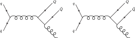
Figure 11: Tree-level Feynman diagrams for the process $q\bar{q}\to Q\bar{Q}(^{3}P_{J}^{[1]})+g$.

The root cause of the breakdown of factorization is that the infrared divergent factor in eq. (61) contains a dependence on the relative momentum $q=(p_{1}-p_{2})/2$ between the heavy quark and antiquark coming from the heavy quark propagator denominator. This dependence cannot be dropped, as doing so will lead to an incorrect result for the singular contribution to the cross section in eq. (62). As can be seen from the Feynman diagram for the process $q\bar{q}\to Q\bar{Q}(^{3}P_{J}^{[1]})+g$ shown in fig. 11, the denominators of eq. (61) come from the virtual heavy quark lines, which have virtualities much smaller than $m$ when the gluon momentum $k$ is soft. Hence, this propagator must be included in the long-distance matrix element. If the $Q\bar{Q}$ is produced with transverse momentum much larger than the soft gluon momentum $k$, we can take the average over the angles of $\bm{k}$ because the effect of variation in $k$ on the kinematics of the quarkonium is at most order $mv$ and can be neglected, and we obtain the usual result in eq. (62). However, in the case where the $Q\bar{Q}(^{3}S_{1}^{[8]})$ is produced at rest and evolves into $Q\bar{Q}(^{3}P_{J}^{[1]})$ plus a soft gluon, the gluon momentum is strongly entangled with the kinematics of the quarkonium as $\bm{k}=-\bm{P}$. In this case, the long-distance matrix element is sensitive to the details of the propagator between the heavy quark and antiquark, which does not allow a description in terms of a local operator product of the heavy quark and antiquark fields. That is, a non-local operator product of the heavy quark and antiquark fields on the same side of the projection operator is needed to describe such processes. To make matters worse, in this case it is not even clear whether it would be possible to isolate the nonlocal operator product of the heavy quark and antiquark fields into a vacuum expectation value, because soft interactions between initial and final state partons will no longer become suppressed, unlike the case of large-$p_{T}$ production. A similar conclusion was obtained in the analysis of transverse-momentum dependent factorization of $P$-wave quarkonium production in ref. Ma:2014oha , where the authors considered the process $gg\to Q\bar{Q}(^{3}P_{J}^{[1]})+X$, which is more complicated because the process $gg\to Q\bar{Q}(^{3}S_{1}^{[8]})$ vanishes at tree level.

As we have shown, this breakdown of NRQCD factorization at $p_{T}\gtrsim 0$ signals a failure of the factorization formalism in terms of local operator matrix elements. This reveals an important distinction between the description of $B$ hadron production in heavy quark effective theory Isgur:1989vq and quarkonium production in NRQCD. In heavy quark effective theory, where long-distance matrix elements involve the $b$ quark field in place of the $Q\bar{Q}$ bilinears, the $b$ quark field is always a local field. In contrast, in quarkonium production nothing prevents the heavy quark and antiquark from being produced nonlocally; this nonlocality can be neglected if it is disentangled from the short-distance process, and in this case we recover the standard form of NRQCD factorization. However this is not always guaranteed to happen, and can fail for production with small transverse momentum as we have seen from the example above.

7 Summary and conclusion

In this work we investigated the application of the shape function formalism for resumming kinematical effects in inclusive production rates of $P$-wave heavy quarkonia. In this formalism, the products of short-distance coefficients and NRQCD matrix elements are replaced by convolutions of short-distance coefficients and shape functions. The shape functions encode the kinematical effects arising from the motion of the heavy quark and antiquark pair in the heavy quarkonium rest frame. They are nonperturbative functions of a lightlike momentum $l$, which corresponds to the difference between the momentum of the quarkonium and the momentum of the heavy quark-antiquark pair. While the formalism was originally developed in refs. Beneke:1997qw ; Fleming:2003gt based on tree-level calculations of quarkonium production, we have extended the application of the formalism to next-to-leading order in the strong coupling, which requires treatment of the ultraviolet divergences that arise from renormalization of NRQCD matrix elements. Due to the mixing between color-singlet and color-octet channels induced by the infrared divergence in the color-singlet $P$-wave production cross section, the short-distance coefficients differ between the NRQCD and shape function formalisms. Based on the perturbative calculations of the shape functions at next-to-leading order accuracy in sec. 3, we have derived in sec. 5 the matching conditions that are valid at one-loop level which allow determination of the short-distance coefficients in the shape function formalism from the standard NRQCD ones. This allows calculation of the cross sections in the shape function formalism at one-loop level using the known NRQCD short-distance coefficients in the $\overline{\rm MS}$ scheme, once the nonperturbative shape functions are known.

In sec. 4 we presented an improved analysis of the nonperturbative shape functions for $P$-wave heavy quarkonia. By using the potential NRQCD formalism developed in refs. Brambilla:2020ojz ; Brambilla:2021abf ; Brambilla:2022rjd ; Brambilla:2022ayc , we reproduced the proposed form of the color-singlet shape function in ref. Beneke:1997qw that is proportional to $\delta(l_{+})$, where $l_{+}$ is the $+$ component of the lightlike momentum $l$ associated with the shape function formalism. Together with the requirement that the normalization of the shape function must be equal to the corresponding NRQCD matrix element, this completely fixes the color-singlet shape function up to corrections suppressed by powers of $v$. In the case of the color-octet shape function, in existing studies it was assumed that it would not be possible to calculate them except within models. While first-principles determinations of the nonperturbative color-octet shape functions may be currently out of reach, we find that the large-$l_{+}$ asymptotic form fixed by the perturbative calculation, and the normalization condition that its integral over $l_{+}$ must reproduce the NRQCD matrix element, strongly constrain the $l_{+}$ dependence of the shape function. Furthermore, we showed through a nonperturbative potential NRQCD calculation of the shape functions that the $l_{+}$ dependence of the color-octet shape functions must be same for all $P$-wave heavy quarkonia, independently of the radial excitation or the heavy quark flavor, up to corrections suppressed by powers of $v$. This strongly constrains the behavior of the shape function, and the model dependence is constrained in the small $l_{+}$ region. As the contribution from the small $l_{+}$ region to the cross section is suppressed, this model dependence has only a small effect on the $P$-wave quarkonium cross section. Hence, the analysis in this work diminishes the model dependence of the shape function formalism for production of $P$-wave heavy quarkonia.

Based on the results for the one-loop perturbative matching conditions and nonperturbative shape functions obtained in this work, we presented two phenomenological applications. First, in section 6.1 we used the fact that the color-octet shape function describes soft-gluon emissions to match the accuracies in $\alpha_{s}$ of the singular radiative corrections near threshold between the color-singlet and color-octet states. This alleviates the problem in fixed-order calculations that, when the short-distance coefficients are computed to same accuracy in the strong coupling, the singular threshold effects are truncated to different orders in $\alpha_{s}$ in the color-octet and color-singlet channels. This can be problematic especially at very large transverse momentum, where the threshold effects can be enhanced. As we have shown in section 6.1, standard NRQCD calculations can yield negative production rates of $\chi_{c}$; the situation is much more improved when we match the singular threshold effects between the two channels using the results from the shape function formalism, and the positivity of the cross sections are ensured to very large values of transverse momentum. While this does not eliminate the need for threshold resummation, the matching of the threshold effects considered in this work can be useful for consistent treatment of threshold resummation throughout the singlet and octet channels.

In section 6.2, we investigated the impact of the nonperturbative shape function on the transverse-momentum dependent cross sections of $\chi_{c}$ and $\chi_{b}$. We employed a variety of model functions for the color-octet shape function to compute the nonperturbative corrections, where the model parameters are constrained by the phenomenologically obtained values of the color-octet matrix elements. As we have argued above, the model dependence only affects the $l_{+}\to 0$ behaviors of the shape functions, and have little effect on the cross sections, so that the model dependence can even be neglected compared to other theoretical uncertainties. We find that at large $p_{T}$, the effect of nonperturbative corrections is mainly to change the overall normalization of the color-octet contribution, which is inconsequential in phenomenology because a change in normalization can be reabsorbed into the color-octet matrix element. This situation gradually changes as we go to lower transverse momentum, and at values of the quarkonium transverse momentum similar or smaller than the heavy quarkonium mass, the cross section in the shape function formalism undershoots the NRQCD prediction by more than the usual size of estimated theoretical uncertainties obtained from scale variations. Although this result is interesting, it is currently not possible to tell whether the shape function formalism gives a better description of the $P$-wave heavy quarkonium cross sections at small $p_{T}$; in the case of $\chi_{c}$, the difference between the two formalisms is not too large compared to the nominal size of relativistic corrections suppressed by $v^{2}$, which is usually taken to be about $0.3$ for charmonium. In the case of $\chi_{b}$, the results from the shape function formalism does tend to agree better with experimental values obtained by extrapolating the feeddown fractions of $\Upsilon$ from $\chi_{b}$ decays to $p_{T}\leq 6$ GeV; nevertheless, actual measurements will be necessary to tell if this is indeed the case.

As we have mentioned, the $P$-wave quarkonium production cross sections are also important for understanding the feeddown contributions in $S$-wave quarkonium production rates. It would also be interesting to apply the shape function formalism for production of $S$-wave quarkonia, such as $J/\psi$, $\psi(2S)$, and $\Upsilon$ states. Production of $S$-wave quarkonia is phenomenologically more significant, and measurements are available for a wider range of transverse momentum. As have been discussed in ref. Brambilla:2022ayc , the color-octet NRQCD matrix elements that appear in $S$-wave quarkonium production rates not only involve logarithmic UV divergences that induce mixing between different color-octet channels, but also quadratic power divergences as well, unlike the $P$-wave case. We can expect that these quadratic power divergences will appear in color-octet shape functions as contributions proportional to $l_{+}$. Since in perturbative QCD these contributions will lead to scaleless power UV divergences, they will need to be subtracted in order to make contact with NRQCD short-distance coefficients that are computed in dimensional regularization. Due to this the nonperturbative shape functions may affect the $S$-wave cross sections differently from $P$-wave cross sections. It would be interesting to see how the application of the shape function formalism will affect $S$-wave quarkonium cross sections.

- (1) G. T. Bodwin, E. Braaten and G. P. Lepage, Rigorous QCD analysis of inclusive annihilation and production of heavy quarkonium, Phys. Rev. D51 (1995) 1125 [hep-ph/9407339].
- (2) M. Butenschoen and B. A. Kniehl, Reconciling production at HERA, RHIC, Tevatron, and LHC with NRQCD factorization at next-to-leading order, Phys. Rev. Lett. 106 (2011) 022003 [1009.5662].
- (3) M. Butenschoen and B. A. Kniehl, World data of J/psi production consolidate NRQCD factorization at NLO, Phys. Rev. D 84 (2011) 051501 [1105.0820].
- (4) M. Butenschoen and B. A. Kniehl, Probing nonrelativistic QCD factorization in polarized photoproduction at next-to-leading order, Phys. Rev. Lett. 107 (2011) 232001 [1109.1476].
- (5) M. Butenschoen and B. A. Kniehl, J/ production in NRQCD: A global analysis of yield and polarization, Nucl. Phys. B Proc. Suppl. 222-224 (2012) 151 [1201.3862].
- (6) M. Butenschoen and B. A. Kniehl, Next-to-leading-order tests of NRQCD factorization with yield and polarization, Mod. Phys. Lett. A 28 (2013) 1350027 [1212.2037].
- (7) M. Butenschoen and B. A. Kniehl, J/psi polarization at Tevatron and LHC: Nonrelativistic-QCD factorization at the crossroads, Phys. Rev. Lett. 108 (2012) 172002 [1201.1872].
- (8) Y.-Q. Ma, K. Wang and K.-T. Chao, production at the Tevatron and LHC at in nonrelativistic QCD, Phys. Rev. Lett. 106 (2011) 042002 [1009.3655].
- (9) B. Gong, L.-P. Wan, J.-X. Wang and H.-F. Zhang, Polarization for Prompt J/ and (2s) Production at the Tevatron and LHC, Phys. Rev. Lett. 110 (2013) 042002 [1205.6682].
- (10) H. Han, Y.-Q. Ma, C. Meng, H.-S. Shao, Y.-J. Zhang and K.-T. Chao, and production at hadron colliders in nonrelativistic QCD, Phys. Rev. D 94 (2016) 014028 [1410.8537].
- (11) G. T. Bodwin, K.-T. Chao, H. S. Chung, U.-R. Kim, J. Lee and Y.-Q. Ma, Fragmentation contributions to hadroproduction of prompt, , and states, Phys. Rev. D 93 (2016) 034041 [1509.07904].
- (12) Y. Feng, B. Gong, C.-H. Chang and J.-X. Wang, Remaining parts of the long-standing polarization puzzle, Phys. Rev. D 99 (2019) 014044 [1810.08989].
- (13) H. S. Chung, Review of quarkonium production: status and prospects, PoS Confinement2018 (2018) 007 [1811.12098].
- (14) N. Brambilla, H. S. Chung, A. Vairo and X.-P. Wang, Production and polarization of -wave quarkonia in potential nonrelativistic QCD, Phys. Rev. D 105 (2022) L111503 [2203.07778].
- (15) H. S. Chung, Quarkonium production and polarization: where do we stand?, EPJ Web Conf. 274 (2022) 01011 [2211.10201].
- (16) N. Brambilla, H. S. Chung, A. Vairo and X.-P. Wang, Inclusive production of , , and states in pNRQCD, 2210.17345.
- (17) M. Butenschoen and B. A. Kniehl, Global analysis of (2S) inclusive hadroproduction at next-to-leading order in nonrelativistic-QCD factorization, Phys. Rev. D 107 (2023) 034003 [2207.09346].
- (18) T. Mannel and G. A. Schuler, Heavy quarkonium effective theory, Z. Phys. C 67 (1995) 159 [hep-ph/9410333].
- (19) I. Z. Rothstein and M. B. Wise, The Octet structure function and radiative quarkonia decays, Phys. Lett. B 402 (1997) 346 [hep-ph/9701404].
- (20) T. Mannel and S. Wolf, QCD based calculation of the semiinclusive decay eta(Q) — gamma + light hadrons, hep-ph/9701324.
- (21) M. Beneke, I. Z. Rothstein and M. B. Wise, Kinematic enhancement of nonperturbative corrections to quarkonium production, Phys. Lett. B 408 (1997) 373 [hep-ph/9705286].
- (22) S. Fleming, A. K. Leibovich and T. Mehen, Resumming the color octet contribution to + , Phys. Rev. D 68 (2003) 094011 [hep-ph/0306139].
- (23) A. Pineda and J. Soto, Effective field theory for ultrasoft momenta in NRQCD and NRQED, Nucl. Phys. B Proc. Suppl. 64 (1998) 428 [hep-ph/9707481].
- (24) N. Brambilla, A. Pineda, J. Soto and A. Vairo, Potential NRQCD: An Effective theory for heavy quarkonium, Nucl. Phys. B566 (2000) 275 [hep-ph/9907240].
- (25) N. Brambilla, D. Eiras, A. Pineda, J. Soto and A. Vairo, New predictions for inclusive heavy quarkonium wave decays, Phys. Rev. Lett. 88 (2002) 012003 [hep-ph/0109130].
- (26) N. Brambilla, D. Eiras, A. Pineda, J. Soto and A. Vairo, Inclusive decays of heavy quarkonium to light particles, Phys. Rev. D 67 (2003) 034018 [hep-ph/0208019].
- (27) N. Brambilla, A. Pineda, J. Soto and A. Vairo, Effective Field Theories for Heavy Quarkonium, Rev. Mod. Phys. 77 (2005) 1423 [hep-ph/0410047].
- (28) N. Brambilla, H. S. Chung and A. Vairo, Inclusive Hadroproduction of -Wave Heavy Quarkonia in Potential Nonrelativistic QCD, Phys. Rev. Lett. 126 (2021) 082003 [2007.07613].
- (29) N. Brambilla, H. S. Chung and A. Vairo, Inclusive production of heavy quarkonia in pNRQCD, JHEP 09 (2021) 032 [2106.09417].
- (30) G. C. Nayak, J.-W. Qiu and G. F. Sterman, Fragmentation, factorization and infrared poles in heavy quarkonium production, Phys. Lett. B 613 (2005) 45 [hep-ph/0501235].
- (31) G. C. Nayak, J.-W. Qiu and G. F. Sterman, Fragmentation, NRQCD and NNLO factorization analysis in heavy quarkonium production, Phys. Rev. D 72 (2005) 114012 [hep-ph/0509021].
- (32) G. C. Nayak, J.-W. Qiu and G. F. Sterman, NRQCD Factorization and Velocity-dependence of NNLO Poles in Heavy Quarkonium Production, Phys. Rev. D 74 (2006) 074007 [hep-ph/0608066].
- (33) M. Beneke, G. A. Schuler and S. Wolf, Quarkonium momentum distributions in photoproduction and B decay, Phys. Rev. D 62 (2000) 034004 [hep-ph/0001062].
- (34) G. T. Bodwin, H. S. Chung, J.-H. Ee, U.-R. Kim and J. Lee, Covariant calculation of a two-loop test of nonrelativistic QCD factorization, Phys. Rev. D 101 (2020) 096011 [1910.05497].
- (35) A. H. Hoang and P. Ruiz-Femenia, Heavy pair production currents with general quantum numbers in dimensionally regularized NRQCD, Phys. Rev. D 74 (2006) 114016 [hep-ph/0609151].
- (36) H. S. Chung, P-wave quarkonium wavefunctions at the origin in the scheme, JHEP 09 (2021) 195 [2106.15514].
- (37) G. T. Bodwin and Y.-Q. Chen, Renormalon ambiguities in NRQCD operator matrix elements, Phys. Rev. D 60 (1999) 054008 [hep-ph/9807492].
- (38) M. Beneke, Perturbative heavy quark - anti-quark systems, PoS hf8 (1999) 009 [hep-ph/9911490].
- (39) M. Beneke, Y. Kiyo and K. Schuller, Third-order correction to top-quark pair production near threshold I. Effective theory set-up and matching coefficients, 1312.4791.
- (40) J. C. Collins and D. E. Soper, Parton Distribution and Decay Functions, Nucl. Phys. B 194 (1982) 445.
- (41) E. Braaten and T. C. Yuan, Gluon fragmentation into heavy quarkonium, Phys. Rev. Lett. 71 (1993) 1673 [hep-ph/9303205].
- (42) E. Braaten, K.-m. Cheung and T. C. Yuan, Z0 decay into charmonium via charm quark fragmentation, Phys. Rev. D 48 (1993) 4230 [hep-ph/9302307].
- (43) T. C. Yuan, Perturbative QCD fragmentation functions for production of P wave mesons with charm and beauty, Phys. Rev. D 50 (1994) 5664 [hep-ph/9405348].
- (44) P. L. Cho, M. B. Wise and S. P. Trivedi, Gluon fragmentation into polarized charmonium, Phys. Rev. D 51 (1995) R2039 [hep-ph/9408352].
- (45) E. Braaten and T. C. Yuan, Gluon fragmentation into spin triplet S wave quarkonium, Phys. Rev. D 52 (1995) 6627 [hep-ph/9507398].
- (46) J. P. Ma, Quark fragmentation into p wave triplet quarkonium, Phys. Rev. D 53 (1996) 1185 [hep-ph/9504263].
- (47) E. Braaten and J. Lee, Next-to-leading order calculation of the color octet 3S(1) gluon fragmentation function for heavy quarkonium, Nucl. Phys. B 586 (2000) 427 [hep-ph/0004228].
- (48) G. T. Bodwin, U.-R. Kim and J. Lee, Higher-order relativistic corrections to gluon fragmentation into spin-triplet S-wave quarkonium, JHEP 11 (2012) 020 [1208.5301].
- (49) Y.-Q. Ma, J.-W. Qiu and H. Zhang, Heavy quarkonium fragmentation functions from a heavy quark pair. I. wave, Phys. Rev. D 89 (2014) 094029 [1311.7078].
- (50) G. T. Bodwin, H. S. Chung, U.-R. Kim and J. Lee, Quark fragmentation into spin-triplet -wave quarkonium, Phys. Rev. D 91 (2015) 074013 [1412.7106].
- (51) Y.-Q. Ma, J.-W. Qiu and H. Zhang, Fragmentation functions of polarized heavy quarkonium, JHEP 06 (2015) 021 [1501.04556].
- (52) V. N. Gribov and L. N. Lipatov, Deep inelastic e p scattering in perturbation theory, Sov. J. Nucl. Phys. 15 (1972) 438.
- (53) L. N. Lipatov, The parton model and perturbation theory, Yad. Fiz. 20 (1974) 181.
- (54) Y. L. Dokshitzer, Calculation of the Structure Functions for Deep Inelastic Scattering and e+ e- Annihilation by Perturbation Theory in Quantum Chromodynamics., Sov. Phys. JETP 46 (1977) 641.
- (55) G. Altarelli and G. Parisi, Asymptotic Freedom in Parton Language, Nucl. Phys. B 126 (1977) 298.
- (56) N. Kidonakis and G. F. Sterman, Resummation for QCD hard scattering, Nucl. Phys. B 505 (1997) 321 [hep-ph/9705234].
- (57) F. Aversa, P. Chiappetta, M. Greco and J. P. Guillet, QCD Corrections to Parton-Parton Scattering Processes, Nucl. Phys. B 327 (1989) 105.
- (58) J. Pumplin, D. R. Stump, J. Huston, H. L. Lai, P. M. Nadolsky and W. K. Tung, New generation of parton distributions with uncertainties from global QCD analysis, JHEP 07 (2002) 012 [hep-ph/0201195].
- (59) G. T. Bodwin, H. S. Chung, U.-R. Kim and J. Lee, Fragmentation contributions to production at the Tevatron and the LHC, Phys. Rev. Lett. 113 (2014) 022001 [1403.3612].
- (60) Y.-Q. Ma, K. Wang and K.-T. Chao, QCD radiative corrections to production at hadron colliders, Phys. Rev. D 83 (2011) 111503 [1002.3987].
- (61) LHCb collaboration, Measurement of the ratio of prompt to production in collisions at TeV, Phys. Lett. B 718 (2012) 431 [1204.1462].
- (62) LHCb collaboration, Study of meson production in collisions at and and observation of the decay , Eur. Phys. J. C 74 (2014) 3092 [1407.7734].
- (63) L.-P. Wan and J.-X. Wang, FDCHQHP: A Fortran package for heavy quarkonium hadroproduction, Comput. Phys. Commun. 185 (2014) 2939 [1405.2143].
- (64) P. L. Cho and A. K. Leibovich, Color octet quarkonia production, Phys. Rev. D 53 (1996) 150 [hep-ph/9505329].
- (65) LHCb collaboration, Measurement of production in collisions at , Eur. Phys. J. C 71 (2011) 1645 [1103.0423].
- (66) LHCb collaboration, Measurement of meson production in collisions at =7 TeV, Eur. Phys. J. C 72 (2012) 2100 [1204.1258].
- (67) Particle Data Group collaboration, Review of Particle Physics, PTEP 2022 (2022) 083C01.
- (68) LHCb collaboration, Forward production of mesons in collisions at and 8TeV, JHEP 11 (2015) 103 [1509.02372].
- (69) N. Brambilla, H. S. Chung, D. Müller and A. Vairo, Decay and electromagnetic production of strongly coupled quarkonia in pNRQCD, JHEP 04 (2020) 095 [2002.07462].
- (70) R. Baier and R. Ruckl, Hadronic Collisions: A Quarkonium Factory, Z. Phys. C 19 (1983) 251.
- (71) A. Petrelli, M. Cacciari, M. Greco, F. Maltoni and M. L. Mangano, NLO production and decay of quarkonium, Nucl. Phys. B 514 (1998) 245 [hep-ph/9707223].
- (72) J. P. Ma, J. X. Wang and S. Zhao, Breakdown of QCD Factorization for P-Wave Quarkonium Production at Low Transverse Momentum, Phys. Lett. B 737 (2014) 103 [1405.3373].
- (73) N. Isgur and M. B. Wise, Weak Decays of Heavy Mesons in the Static Quark Approximation, Phys. Lett. B 232 (1989) 113.