Analyzing variational quantum landscapes with information content

Abstract

The parameters of the quantum circuit in a variational quantum algorithm induce a landscape that contains the relevant information regarding its optimization hardness. In this work we investigate such landscapes through the lens of information content, a measure of the variability between points in parameter space. Our major contribution connects the information content to the average norm of the gradient, for which we provide robust analytical bounds on its estimators. This result holds for any (classical or quantum) variational landscape. We validate the analytical understating by numerically studying the scaling of the gradient in an instance of the barren plateau problem. In such instance we are able to estimate the scaling pre-factors in the gradient. Our work provides a new way to analyze variational quantum algorithms in a data-driven fashion well-suited for near-term quantum computers.

I Introduction

Variational quantum algorithms (VQAs) have been marked as a promising path towards quantum advantage in pre-fault-tolerant quantum hardware. In nearly a decade of research since its original proposal [1], the field of VQAs has seen significant progress both theoretical and experimentally [2, 3]. It is yet to be seen if noisy intermediate-scale quantum (NISQ) [4] devices are able to reach unambiguous quantum advantage through VQA. Issues such as vanishing gradients or barren plateaus (BP) [5, 6, 7, 8], the expressivity of the quantum circuits [9, 10, 11] or difficulties optimizing a noisy cost function [12] are only a few examples of the hurdles faced by VQA which reduce the hope of quantum advantage in the near-term.

From a computer science point-of-view VQAs are a fascinating object of study. They can be considered classical cost functions with classic input/output. Yet the cost function might not be classically accessible in general. So far, there is no clear evidence that optimizing a VQA is feasible with standard optimization methods [12]. Some researchers have attempted to close this gap by developing new optimizers tailored to quantum circuits [13, 14] or use machine learning techniques to assist during the optimization [15, 16] with inconclusive results. More recently an attempt to visualize the optimization landscape by dimensionality reduction techniques was proposed [17]. Still, little is known about the features of variational quantum landscapes and how to extract them.

Landscape analysis aims at characterizing the landscape of cost functions by efficiently sampling the parameter space to understand the “hardness” of the optimization problem [18, 19, 20, 21, 22, 23]. For a VQA this implies only classical post-processing of data from a quantum device. In contrast, the optimization step of a VQA involves constant interaction between quantum and classical resources. In NISQ hardware such interactions might come with a large overhead. To the best of our knowledge, no prior work on data-driven landscape analysis exists in the context of VQA.

In this work, we aim to close the gap between VQA and landscape analysis through the information content (IC) [24] of the quantum landscape. We demonstrate the connection between IC and the average norm of the gradient of the landscape. We derive robust lower/upper bounds of this quantity which provides a crucial understanding of the landscape (e.g. complexity of optimizing the cost function). We apply our results to numerically study the BP problem for local and global cost functions from ref. [6], showing excellent agreement with theoretical asymptotic scaling in the size of the gradient. Also, we demonstrate how to calculate pre-factors of the asymptotic scaling, which are in practice more relevant for implementing algorithms. As far as we know, this is the first work where scaling pre-factors are calculated in the context of VQAs and BPs.

The manuscript is organized as follows. In Section II we give background on VQAs and IC. We connect the average norm of the gradient with IC in Section III, followed by a numerical diagnosis of BP using IC in  Section IV. Section VI addresses the estimation of pre-factors in the scaling of BP. In Section VII we discuss the implications of our results and point out future directions.

II Background

II.1 Parameterized Quantum Circuits

In a variational quantum algorithm one aims at exploring the space of quantum states by minimizing a cost function with respect to a set of tunable real-valued parameters $\vec{\theta}\in[0,2\pi)^{m}$ of a parametrized quantum circuit (PQC). A PQC evolves an initial quantum state $\ket{\psi_{0}}$ to generate a parametrized state

$$\ket{\psi(\vec{\theta})}=U(\vec{\theta})\ket{\psi_{0}},$$ (1)

where $U(\vec{\theta})$ is a unitary matrix of the form

$$U(\vec{\theta})=\prod_{i=1}^{m}U_{i}(\vec{\theta}_{i})W_{i},$$ (2)

with

$$U_{i}(\vec{\theta}_{i})=\exp\left(-i\vec{\theta}_{i}V_{i}\right).$$ (3)

Here $W_{i}$ are fixed unitary operations and $V_{i}$ are hermitian matrices. In a VQA these parameters are driven by (classically) minimizing a cost function $C(\vec{\theta})$, built as the expectation value of a quantum observable $\hat{O}$,

$$C(\vec{\theta})=\bra{\psi_{0}}U^{\dagger}(\vec{\theta})\hat{O}U(\vec{\theta})\ket{\psi_{0}}.$$ (4)

A successful optimization reaches an approximation to the lowest eigenvalue of $\hat{O}$, and the optimal parameters represent an approximation to its ground-state [3, 2]. Our object of study is the manifold defined by a PQC and $\hat{O}$ which we call a variational quantum landscape.

II.2 Information content

The information content (IC) of a variational landscape is a measure of its variability between two nearby randomly-chosen points therein [25]. For this feature, high (low) IC relates to the ruggedness (flatness) of the landscape [26].

Definition 1 (Information Content (IC))

Given a finite symbolic sequence $\phi=\{-,\odot,+\}^{S}$ of length $S$ and let $p_{ab},a\neq b\in\{-,\odot,+\}$ denote the probability that $ab$ occurs in the consecutive pairs of $\phi$. The information content is defined as

$$H=\sum_{a\neq b}h\left(p_{ab}\right),$$ (5)

with

$$h(x)=-x\log_{6}x.$$ (6)

In this definition pairs of the same symbols are excluded, leaving only six combinations,

$$p_{ab}=\{p_{+-},p_{-+},p_{+\odot},p_{\odot+},p_{-\odot},p_{\odot-}\}.$$ (7)

The $\log_{6}$ is necessary to ensure $H\leq 1$.

To compute the IC, we use the algorithm given in ref. [26]: (1) Sample $M(m)\in\mathcal{O}(m)$ points of the parameter space $\Theta=\{\vec{\theta}_{1},\dots,\vec{\theta}_{M}\}\in[0,2\pi)^{m}$. (2) Measure $C(\vec{\theta}_{i})$ on a quantum computer (this is the only step where it is needed). (3) Generate a random walk $W$ of $S+1<M(m)$ steps over $\Theta$, and compute the finite-size approximation of the gradient at each step $i$ $$\Delta C_{i}=\frac{C(\vec{\theta}_{i+1})-C(\vec{\theta}_{i})}{\norm{\vec{\theta}_{i+1}-\vec{\theta}_{i}}}.$$ (8) (4) Create a sequence $\phi(\epsilon)$ by mapping $\Delta C_{i}$ onto a symbol in $\{-,\odot,+\}$ with the rule $$\phi(\epsilon)=\begin{cases}-&\text{ if }\Delta C_{i}<-\epsilon\\ \odot&\text{ if }|\Delta C_{i}|\leq\epsilon\\ +&\text{ if }\Delta C_{i}>\epsilon\end{cases}$$ (9) (5) Compute the empirical IC (denoted as $H(\epsilon)$ henceforth) by applying Definition 1 to $\phi(\epsilon)$. (6) Repeat these steps for several values of $\epsilon$.

III Connection between information content and norm of the gradient

This section shows the relation between IC and the average norm of the gradient, from now denoted as $\norm{\nabla C}$. We take advantage of the fact that each step is isotropically random in $W$. This allows us to derive the underlying probability of $\Delta C_{i}$. Additionally, we use IC to bound the probability of pairs of symbols appearing along $W$ which allows us to estimate $\norm{\nabla C}$. Although we demonstrate our results for a variational quantum landscape, they extend to any optimization landscape.

III.1 Estimation of the norm of the gradient

The random walks $W$ over $\Theta$ satisfy

$$\norm{\vec{\theta}_{i+1}-\vec{\theta}_{i}} \leq d$$ (10)

$$\frac{\vec{\theta}_{i+1}-\vec{\theta}_{i}}{\norm{\vec{\theta}_{i+1}-\vec{\theta}_{i}}} =\vec{\delta}_{i},$$ (11)

where $\vec{\delta}_{i}$ is drawn from the isotropic distribution and $d$ is fixed before starting the walk but might be varied. By Taylor expanding Equation 8 and the mean-value theorem, the finite-size gradient can be written as

$$\Delta C_{i}=\nabla C((1-t)\vec{\theta}_{i}+t\vec{\theta}_{i+1})\cdot\vec{\delta}_{i},$$ (12)

with $t\in(0,1)$. Since the sampled points $\Theta$ are chosen randomly, we can assume that $\Delta C$ and $\nabla C(\vec{\theta})\cdot\vec{\delta}$ are drawn from the same probability distribution, given a sufficiently large $\Theta$.

The isotropic condition of $W$ allows us to calculate the probability distribution of $\nabla C(\vec{\theta})\cdot\vec{\delta}$:

Lemma 1

Let $C(\vec{\theta})$ be a differentiable function for all $\vec{\theta}\in[0,2\pi)^{m}$. Let $\vec{\delta}\in\mathbb{R},\|\vec{\delta}\|=1$ be drawn from the isotropic distribution. Then $(\nabla C(\vec{\theta})\cdot\vec{\delta})^{2}$ is a random variable with a beta probability distribution $(\operatorname{\mathcal{B}})$ [27] such that

$$\left(\nabla C(\vec{\theta})\cdot\vec{\delta}\right)^{2}\sim\norm{\nabla C(\vec{\theta})}^{2}\operatorname{\mathcal{B}}\left(\frac{1}{2},\frac{m-1}{2}\right).$$ (13)

The proof can be found in Section A.1.

We can use Lemma 1 to bound the probability of $\nabla C(\vec{\theta})$ from the $\operatorname{\mathcal{B}}$ cumulative distribution function (CDF).

Theorem 1 (CDF of $\nabla C(\vec{\theta})\cdot\vec{\delta}$)

Let $C(\vec{\theta})$ be a differentiable function at every $\vec{\theta}\in[0,2\pi)^{m}$. Let $\vec{\delta}\in\mathbb{R},\|\vec{\delta}\|=1$ be drawn from the isotropic distribution. Then $\nabla C(\vec{\theta})\cdot\vec{\delta}$ is a random variable with cumulative density function

$$\operatorname{\rm Prob}\left(\nabla C(\vec{\theta})\cdot\vec{\delta}\leq\epsilon\right)=\\ \frac{1}{2}\left(1+\operatorname{sgn}(\epsilon)\ \mathcal{I}\left(\frac{\epsilon^{2}}{\norm{C(\vec{\theta})}^{2}};\frac{1}{2},\frac{m-1}{2}\right)\right),$$ (14)

where $\mathcal{I}(x;\alpha,\beta)$ is the regularized incomplete beta function with parameters $\alpha$ and $\beta$.

The proof of this theorem can be found in Section A.2.

Lemma 1 implies:

$$\operatorname{\mathbb{E}}_{W}\left(\left(C(\vec{\theta})\cdot\vec{\delta}\right)^{2}\right)\sim\\ \operatorname{\mathbb{E}}_{W}\left(\norm{\nabla C(\vec{\theta})}^{2}\right)\operatorname{\mathcal{B}}\left(\frac{1}{2},\frac{m-1}{2}\right),$$ (15)

where $\operatorname{\mathbb{E}}_{W}$ denotes the expectation taken over the points in random walk $W$. As an immediate consequence, we have the CDF of $\nabla C(\vec{\theta})\cdot\vec{\delta}$ averaged over a $W$:

Corollary 1 (CDF of average norm of gradients)

Let $C(\vec{\theta})$ be a differentiable function at every $\vec{\theta}\in[0,2\pi)^{m}$. Let $\vec{\delta}\in\mathbb{R},\|\vec{\delta}\|=1$ be drawn from the isotropic distribution. Then $\nabla C(\vec{\theta})\cdot\vec{\delta}$ is a random variable with cumulative density function

$$\operatorname{\rm Prob}\left(\operatorname{\mathbb{E}}_{W}\left(\nabla C(\vec{\theta})\cdot\vec{\delta}\right)\leq\epsilon\right)\equiv\operatorname{\Phi}_{m}\left(\epsilon\right)=\\ \frac{1}{2}\left(1+\operatorname{sgn}(\epsilon)\mathcal{I}\left(\frac{\epsilon^{2}}{\norm{\nabla C}_{W}^{2}};\frac{1}{2},\frac{m-1}{2}\right)\right),$$ (16)

with

$$\norm{\nabla C}^{2}_{W}=\operatorname{\mathbb{E}}_{W}\left(\norm{\nabla C(\vec{\theta})}^{2}\right).$$ (17)

The corollary can be easily proved by extending the proof of Theorem 1 (see Section A.2).

Note that $\norm{\nabla C}_{W}$ converges to the average norm of the gradient over $[0,2\pi)^{m}$, i.e., $\norm{\nabla C}^{2}\coloneqq\operatorname{\mathbb{E}}||\nabla C(\vec{\theta})||^{2}$ at a rate [28]:

$$\bigg{|}\norm{\nabla C}-\norm{\nabla C}_{W}\bigg{|}\in\mathcal{O}_{p}(M^{-1/2}),$$ (18)

allowing us to approximate the interesting $\norm{\nabla C}_{W}$ with the accessible $\norm{\nabla C}_{W}$ with small error.

III.2 Probability concentration for information content

Our next goal is to bound the probability of pairs of symbols appearing in $\phi$ in two regimes: high and low IC.

High information content

If one interprets IC as a partial entropy of the landscape, high $H$ necessarily implies approximately equal probabilities $p_{ab}$. Therefore, a minimal concentration of probabilities must exist such that a high value of $H$ can be reached. One can formally define this statement;

Lemma 2

Let $H>2h(1/2)$ be the IC of a given sequence $\phi$. Consider the probabilities in Equation 7 such that the sum of any four of them ($p_{4}$) is bounded by

$$p_{4}\geq 4q,$$ (19)

with $q$ the solution of $H=4h(x)+2h(1/2-2x)$.

The proof can be found in Section A.3. The bound on $p_{4}$ in the above lemma gets tighter as $q$ increases, and so does $H$, which by definition $H\leq 1$.

The empirical IC $H(\epsilon)$ computed from step 5 of the algorithm in Section II.2 peaks at the maximum IC (MIC) [25, 26],

$$H_{M}=\max_{\epsilon}H(\epsilon),$$ (20)

where $\epsilon_{\rm M}$ denotes the parameter at the peak.

Low information content

For a low IC to occur, all $p_{ab}$ must be small, and their values can be upper-bounded.

Lemma 3

Let $H$ be the IC with bound $H\leq\eta\leq 1/6$ of a given sequence $\phi$. Then the probability of consecutive $\odot$ steps during a random walk are close to $1$ by the expected norm of the gradient is bounded by

$$p_{\odot\odot}\geq 1-3\eta,$$ (21)

The proof can be found in Section A.4.

The point where $H(\epsilon)\leq\eta$ is defined as sensitivity IC (SIC) [25, 26],

$$H_{S}=\min\left\{\epsilon>0|H(\epsilon)\leq\eta\right\},$$ (22)

with $\epsilon_{\rm S}$, sensitivity, its $\epsilon$. The SIC identifies the $\epsilon$ at which (almost) all symbols in $\phi_{i}$ are $\odot$. All symbols become exactly $\odot$ when $\eta=0$.

III.3 Information content to estimate the norm of the gradient

We are ready to show the main result of this work. We make use of the results in Section III.1 and Section III.2 to prove that $H(\epsilon)$ estimates the average norm of the gradient $\norm{\nabla C}$ for any classical or quantum landscape. To the best of our knowledge, this is the first time, including the field of classical optimization, where such bounds are calculated.

First, we relate $H_{M}$ to the norm of the gradient. High values of IC guarantee a minimal probability for individual steps to increase and decrease and thus bounds the compatible values of $\epsilon/\norm{\nabla C}_{W}$.

Theorem 2 ($H_{M}$ bounds $\norm{\nabla C}_{W}$)

Let $H_{M}$ be the empirical MIC of a given function $C(\vec{\theta})$, and $\epsilon_{\rm M}$ its corresponding $\epsilon$. Let $q$ be the solution to the equation $H_{M}=4h(x)+2h(1/2-2x)$. Then,

$$\frac{-\epsilon_{\rm M}}{\Phi_{m}^{-1}(2q)}\leq\norm{\nabla C}_{W}\leq\frac{-\epsilon_{\rm M}}{\Phi_{m}^{-1}\left(\frac{1-2q}{2}\right)}.$$ (23)

The proof is given in Section A.5.

The second result connects SIC to the bounds in the norm of the gradient. Small values of IC imply a large probability of consecutive $\odot$ steps in $\phi_{i}$ or equivalently small probabilities for $p_{ab}$. When this occurs, then $\epsilon_{\rm S}$ is used to upper bound $\norm{\nabla C}_{W}$.

Theorem 3 ($H_{S}$ upper bounds $\norm{\nabla C}_{W}$)

Let $H_{S}$ be the empirical SIC of a given function $C(\vec{\theta})$, and $\epsilon_{\rm S}$ its corresponding $\epsilon$. Then

$$\norm{\nabla C}_{W}\leq\frac{-\epsilon_{\rm S}}{\Phi_{m}^{-1}\left(3\eta/2\right)}.$$ (24)

The proof is given in Section A.6.

From Equation 18, it is obvious that $\norm{\nabla C}_{W}$ well approximate $\norm{\nabla C}$ for a large $M$. Hence, we can use Theorem 2 and Theorem 3 to bound $\norm{\nabla C}$ with a long sequence $\phi$.

Theorem 2 and Theorem 3 provide confidence intervals of $\norm{\nabla C}$ without prior knowledge of the variational landscape. The former gives both an upper and lower bound of $\norm{\nabla C}$ but can only be applied when $H$ has a minimum value, while the latter is always applicable with an arbitrary small $\eta$ for an upper bound.

It is known that the beta distribution (with the parametrization in Lemma 1) converges to a normal distribution [29]:

$$\lim_{m\rightarrow\infty}\operatorname{\Phi}_{m}\left(\frac{\epsilon}{\norm{\nabla C}}\right)=\Phi_{G}\left(\frac{\epsilon\sqrt{m}}{\norm{\nabla C}}\right),$$ (25)

where $\Phi_{G}(\cdot)$ is the CDF of the standard normal distribution. From it, we can naturally interpret the functionality of $\sqrt{m}$ as dimensionality normalization in our bounds.

IV Information content to diagnose barren plateaus

Our goal is now to apply the previous results to study the problem of barren plateaus (BP) [5, 6] We choose this problem because there exist analytical results on the scaling of the $\norm{\nabla C}$. This allows us to directly verify that $H(\epsilon)$ can be used as a proxy to $\norm{\nabla C}$.

BPs are characterized by the following conditions [5],

$$\mathbb{E}\left(\partial_{k}C(\vec{\theta})\right) =0,$$ (26)

$${\rm Var}\left(\partial_{k}C(\vec{\theta})\right) \in\mathcal{O}\left(\exp(-n)\right),$$ (27)

where $n$ is the number of qubits. BP implies exponentially vanishing variances of the derivatives. Similarly, BP can be understood as having a flat optimization landscape. These two concepts are connected by Chebyshev’s inequality [30].

The IC allows us to calculate

$$\norm{\nabla C}\approx\operatorname{\mathbb{E}}_{W}\left(\sum_{k=1}^{m}(\partial_{k}C(\vec{\theta}))^{2}\right)=\sum_{k=1}^{m}{\rm Var}_{W}(\partial_{k}C(\vec{\theta})),$$ (28)

where ${\rm Var}_{W}$ computes the variance over points of the random walk $W$. Hence, IC is a proxy of the average variance of each partial derivative in the parameter space.

V Numerical experiments

To showcase IC as a tool to analyze the landscape of a VQA, we perform a numerical study of the BP problem as described by Cerezo et al. in [6]. Here, the authors analytically derive the scaling of ${\rm Var}(\partial C(\vec{\theta}))$ in two different scenarios. Such scaling depends both on the qubit size and circuit depth of the PQC. If the cost function is computed from global observables (e.g. non-trivial support on all qubits), BPs exist irrespective of the depth of the PQC. In the case of local observables (e.g. non-trivial support on a few qubits), one can train shallow PQCs, but BPs gradually appear as the circuit depth increases. These results hold for alternating layered ansatze composed of blocks of 2-local operations (Fig. 4 in [6]).

In our numerical experiments, we use circuits from 2 to 14 qubits, each of them going from 4 to 16 layers. We calculate the cost function from

$$\hat{O}_{\rm Local}=\frac{1}{n}\sum_{i=1}^{n}(1-Z_{i})$$ (29)

$$\hat{O}_{\rm Global}=\bigotimes_{i=1}^{n}\ket{0}\bra{0}^{\otimes n}.$$ (30)

Further details of the numerical experiments are given in Appendix B.

The results of the BP problem using IC are shown in Figure 2. In all plots we compute the bounds on the $\norm{\nabla C}$ from Theorem 2 (solid lines) and Theorem 3 (dashed lines), for the local (blue) and global (orange) cost functions. Additionally we show the value of $\epsilon_{\rm M}\cdot\sqrt{m}$ (dots) and $\epsilon_{\rm S}\cdot\sqrt{m}$ (crosses).

The first trend we observe is that the $\norm{\nabla C}$ shows two different scalings with respect to qubits (left panels) and layers (right panels). The scaling with qubits shows a $\mathcal{O}({\rm poly^{-1}}(n))$ decay in the local cost function and a remarkable $\mathcal{O}({\exp(-n)})$ decay with the global cost function. We emphasize the fact that these results are in perfect agreement with the predictions in [6]. On the other hand, the scaling with layers strongly depends on the number of qubits. For 4 qubits, $\hat{O}_{\rm Global}$ has a constant value $\norm{\nabla C}\approx 10^{-2}$, while $\hat{O}_{\rm Local}$ shows a small decay with a similar average. For 10 and 14 qubits, we recover the predicted $\mathcal{O}({\rm poly^{-1}}(n))$ decay in the $\hat{O}_{\rm Local}$. In contrast, $\hat{O}_{\rm Global}$ has $\norm{\nabla C}\approx 10^{-4}-10^{-6}$ $\hat{O}_{\rm Global}$ which is already close to float precision. Finally, we observe that $\epsilon_{\rm M}\cdot\sqrt{m}$ is close to the lower bound, thus making it a robust proxy for $\norm{\nabla C}$.

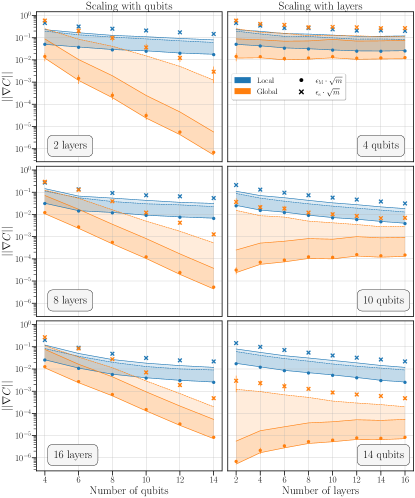
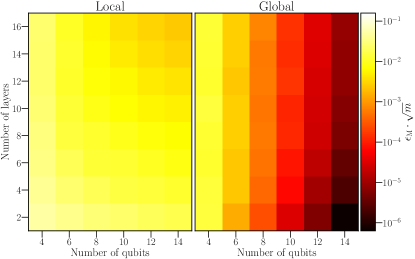
Figure 1: Scaling of the average gradient $\norm{\nabla C}$ with respect to qubits (left panel) and layers (right panel). The solid lines show the bounds from Equation 23 (solid lines) and Equation 24 (dashed lines). $\norm{\nabla C}$ can take values within the shadow areas in between these lines. The markers refer to the values of $\epsilon_{\rm M}\cdot\sqrt{m}$ (dots) and $\epsilon_{\rm S}\cdot\sqrt{m}$ (crosses). They are calculated from the median of five independent runs, with their standard deviation as the error bars. The colors represent the results for the local (blue) and global (orange) cost functions.

Figure 2: Heatmap of $\epsilon_{\rm M}\cdot\sqrt{m}$ for local (left panel) and global (right panel) cost functions. The number of qubits is depicted on the x-axis, while the number of layers is shown on the y-axis.

In Figure 2 we show a heatmap of the values of $\epsilon_{\rm M}\cdot\sqrt{m}$ when increasing the number of qubits (x-axis) and the layers (y-axis) for both local (left) and global (right) cost function. The values of results for $\hat{O}_{\rm Local}$ (left panel) show a rich variety of features: for 2 to 6 layers $\epsilon_{\rm M}\cdot\sqrt{m}$ shows a very mild decay, but for more than 8 layers the decay sharpens. This is exactly as expected for local cost functions: BPs appear gradually as the circuit depth increases. We speculate that the color change at the top right corner of the left panel in Figure 2 corresponds to a transition regime. With regard to the global cost function (right panel), the expected exponential decay (in the number of qubits) is observed.

Surprisingly, both Figure 2 and 2 show an increase in $\epsilon_{\rm M}\cdot\sqrt{m}$ (or equivalently $\norm{\nabla C}$) at a fixed number of qubits as the number of layers grows for the global cost function. We have not been able to find an explanation for this behavior either analytically or in the literature. However, this is an example of how data-driven methods might provide useful insight for deeper understanding.

VI Estimation of scaling pre-factor

Global cost function prefactors
$f(n)=2^{\alpha n+\beta}$
	$\alpha$		$\beta$
Layers	LB	$\epsilon_{\rm M}\cdot\sqrt{m}$	LB	$\epsilon_{\rm M}\cdot\sqrt{m}$
2	-1.43	-1.41	-0.91	-0.68
4	-1.29	-1.27	-1.22	-1.09
6	-1.19	-1.17	-1.85	-1.68
8	-1.13	-1.12	-1.98	-1.85
10	-1.12	-1.12	-1.97	-1.82
12	-1.06	-1.05	-2.41	-2.26
14	-1.07	-1.07	-2.29	-2.14
16	-1.06	-1.06	-2.25	-2.10

Table 1: Estimated qubit scaling pre-factors of the global cost function by linear fitting. $\alpha$ is the slope and $\beta$ the intercept of the linear model. Each coefficient has two columns showing the results of fitting $\epsilon_{\rm M}\cdot\sqrt{m}$ and its lower bound (LB).

Local cost function scaling with qubits
$f^{-1}(n)=\alpha n^{2}+\beta n+\gamma$
	$\alpha$		$\beta$		$\gamma$
Layers	LB	$\epsilon_{\rm M}\cdot\sqrt{m}$	LB	$\epsilon_{\rm M}\cdot\sqrt{m}$	LB	$\epsilon_{\rm M}\cdot\sqrt{m}$
2	0.05	0.03	2.80	3.3	8.05	6.37
4	-0.25	-0.24	10.08	10.22	-12.86	-12.96
6	-0.16	-0.16	11.09	11.52	-11.37	-12.16
8	-0.27	-0.30	16.20	16.99	-26.22	-28.13
10	-0.56	-0.55	25.33	25.63	-57.30	-57.50
12	-0.31	-0.34	25.52	26.77	-56.33	-59.65
14	0.14	0.08	25.99	28.00	-69.42	-75.87
16	0.13	0.12	33.69	34.95	-104.77	-108.92

Table 2: Estimated qubit scaling pre-factors of the local cost function by fitting a second-degree polynomial. Each coefficient has two columns showing the results of fitting $\epsilon_{\rm M}\cdot\sqrt{m}$ and its lower bound (LB).

Local cost function scaling with layers
$f^{-1}(l)=\alpha l^{2}+\beta l+\gamma$
	$\alpha$		$\beta$		$\gamma$
Qubits	LB	$\epsilon_{\rm M}\cdot\sqrt{m}$	LB	$\epsilon_{\rm M}\cdot\sqrt{m}$	LB	$\epsilon_{\rm M}\cdot\sqrt{m}$
4	-0.1	-0.11	3.29	3.5	12.74	12.43
6	-0.27	-0.28	9.54	9.94	6.26	6.10
8	0.13	0.13	7.69	7.98	18.80	19.16
10	0.48	0.52	5.98	5.89	27.79	29.72
12	0.81	0.82	4.68	5.04	38.24	38.70
14	1.14	1.18	2.95	3.04	48.93	50.89

Table 3: Estimated layer scaling pre-factors of the local cost function by fitting a second-degree polynomial. Each coefficient has two columns showing the results of fitting $\epsilon_{\rm M}\cdot\sqrt{m}$ and its lower bound (LB).

Thus far the numerical results have just confirmed the asymptotic theoretical predictions of the considered BP problem. Our methodology can be used beyond the asymptotic scaling to compute actual pre-factors by fitting $\epsilon_{\rm M}\cdot\sqrt{m}$ to its predicted functional form, including bounds on them from Equation 23. Obtaining such pre-factors is challenging analytically. Yet they are relevant when studying the complexity of an algorithm in practice. In this section, we obtain the scaling pre-factors for the global cost function (in the number of qubits) and the local cost function for the number of qubits and layers (see Appendix B for additional details of these fittings).

First, we study the global cost function scaling with qubits for each number of layers in our data. We fit a linear model $f(x)=\alpha x+\beta$ with $x=\rm{log}_{2}(\epsilon_{\rm M}\cdot\sqrt{m})$. The results of the fit are shown in Table 3. For each of the coefficients, we show the fitting values of the lower bound (LB column) and $\epsilon_{\rm M}\cdot\sqrt{m}$ (right column). As the number of layers increases, $\alpha\rightarrow-1.0$, which is consistent with exponential decay of the form $2^{-n}$ predicted in [6]. More importantly, asymptotic scaling is not sensitive to the constant factor $\beta$, but it is given by the right column in Table 3. Based on the trend in this column we speculate that the constant factor is $\beta\rightarrow-2.0$.

In the case of $\hat{O}_{\rm Local}$, there are fewer known asymptotic predictions of the gradient norm. In [6] it is shown that there exist three regimes: trainable, BPs, and transition area, depending on the depth with respect to the system size. Due to the small number of qubits and layers of our numerical study, we assume to be in the trainable regime, where theory predicts a $\norm{\nabla C}$ scaling in $\mathcal{O}({\rm{poly}^{-1}}(n))$. We use a second-order polynomial model $f(n)=\alpha n^{2}+\beta n+\gamma$ to fit $(\epsilon_{\rm M}\cdot\sqrt{m})^{-1}$. The results are given in Table 3. The first observation is the small value of the quadratic coefficient for all layers. This might lead to thinking that a linear function will be better suited. To discard this possibility we perform a linear fit (see Figure 4 in Appendix B) leading to comparable values of the slope and intercept, with slightly better fitting statistics for the second-degree polynomial. The $\beta$ coefficient shows a 10-fold increase as the number of layers grows. In contrast, $\gamma$ gets increasingly more negative with the number of layers. Note that we can extract the degree of the polynomial, which is impossible from the theory.

Lastly, we estimate the scaling coefficients of the local cost function with respect to layers, where no theoretical scaling is known [6]. We choose a second-order polynomial as the hypothesis functional form to fit the data. A linear model clearly under-fits the data (see Figure 5), thus confirming the intuition of a higher-order polynomial scaling. The results are presented in Table 3. The quadratic coefficient $\alpha$ increases as the number of qubits grows at $n\geq 8$, and so does the constant term $\gamma$. In contrast, the linear term $\beta$ remains roughly constant across all system sizes studied. An opposite trend in the coefficients seems to occur between $n=4$ and $n=6$, $\alpha$ and $\gamma$ decrease, while $\beta$ increases. We have not been able to match this change in the tendency to a change in scaling, leaving a finite-size effect in the fitting as the most possible explanation.

The results presented in this section are a demonstration that data-driven approaches can provide useful insight to complement analytical methods and can be leveraged to get a deeper understanding of a problem.

VII Conclusions

Variational quantum algorithms have been intensively studied as a suitable application for near-term quantum hardware. From a computer science perspective, they are simply an optimization problem with classical input/output, yet their cost function is a quantum object. The parameters of any optimization problem induce a landscape that contains information about its “hardness”. Landscape analysis is central to classical optimization but has been somewhat ignored in the VQAs community.

In this work, we investigate the information content features of a variational quantum landscape, which can be calculated efficiently by sampling the parameter space. We prove that for any (classical or quantum) cost function the average norm of its gradient can be rigorously bounded with the information content. We validate our theoretical understating by a numerical experiment, confirming the predicted asymptotic scaling of the gradient in the barren plateau problem. Finally, we apply our results to predict scaling pre-factors of the gradient in a data-driven fashion. To our knowledge, this is the first time that such pre-factors are calculated for a VQA.

The study of optimization landscapes of VQA opens a new avenue to explore their capabilities within the NISQ era. First, landscape analysis does not require constant interaction between quantum and classical hardware. Secondly, only linear (in the number of parameters) queries to a quantum computer suffice to extract the information content instead of polynomially many queries for a standard optimization routine. Finally, information content might be used as an easy and comparable metric between ansatzes.

We envision future research directions with information content such as studying the feasibility of the VQA optimization, estimating the number of shots needed to resolve a gradient, or warm-starting the algorithm from regions of interest in parameter space. Therefore we anticipate that landscape analysis and information content might have a broad range of applications beyond VQAs in the NISQ era.

Author contribution

The project was conceived by XBM and HW. APS and HW proved the theorems, corollaries, and lemmas. XBM performed the numerical simulations with assistance from APS and HW. XBM analyzed the data and performed the model fits. All the authors interpreted the results and wrote the manuscript.

Competing interests

The authors declare no competing interests.

Data availability

The data to reproduce the results of this work can be found in Zenodo [31].

Appendix A Proofs

A.1 Proof of Lemma 1

The main assumption of Lemma 1 is $\vec{\delta}$ is drawn from the isotropic distribution on the unit sphere in $m$ dimensions. As a first step, we use the spherical symmetry of the parameter space to align the first coordinate of $\vec{\delta}$ with the vector $\nabla C(\vec{\theta})$. Thus,

$$\left(\nabla C(\vec{\theta})\cdot\vec{\delta}\right)^{2}=\norm{\nabla C(\vec{\theta})}^{2}\delta_{1}^{2}.$$ (31)

Now, we redefine the isotropic distribution as the normalized multi-dimensional Gaussian distribution ($\mathcal{N}$),

$$\vec{\delta}=\frac{\vec{x}}{\norm{\vec{x}}};\qquad{\rm with}\;\vec{x}\sim\mathcal{N}(0,\mathbb{I}^{m}).$$ (32)

By definition, each of the coordinates-squared in the multi-dimensional Gaussian distribution follows a $\chi^{2}$ distribution [32]. In particular, $x_{1}^{2}\sim\chi^{2}(1)$, and $\sum_{i=2}^{m}x_{i}^{2}\sim\chi^{2}(m-1)$. It is well-known [27] that the above quotient follows a beta distribution with parameters $1/2$ and $(m-1)/2$, i.e.,

$$\left(\nabla C(\vec{\theta})\cdot\vec{\delta}\right)^{2}=\norm{\nabla C(\vec{\theta})}^{2}\frac{x_{1}^{2}}{x_{1}^{2}+\sum_{i=2}^{m}x_{i}^{2}}\sim\norm{\nabla C(\vec{\theta})}^{2}\operatorname{\mathcal{B}}\left(\frac{1}{2},\frac{m-1}{2}\right),$$ (33)

finishing the proof. $\square$

A.2 Proof of Theorem 1

The CDF of a beta distribution is the regularized incomplete beta function $\mathcal{I}$. Thus, in the assumptions of Lemma 1,

$$\Pr(\left(C(\vec{\theta})\cdot\vec{\delta}\right)^{2}\leq\epsilon^{2})=\mathcal{I}\left(\frac{\epsilon^{2}}{||\nabla C(\vec{\theta})||^{2}},\frac{1}{2},\frac{m-1}{2}\right),$$ (34)

where $\epsilon$ is a realization of $(\nabla C(\vec{\theta})\cdot\vec{\delta})^{2}$.

We are however interested in $\nabla C(\vec{\theta})\cdot\vec{\delta}$. From the isotropic condition of $\vec{\delta}$, it is immediate that $\nabla C(\vec{\theta})\cdot\vec{\delta}$ is symmetric with respect to $0$. Using this observation,

$$\Pr(|C(\vec{\theta})\cdot\vec{\delta}|\leq\epsilon) =\Pr(-\epsilon\leq\nabla C(\vec{\theta})\cdot\vec{\delta}\leq 0)+\Pr(0\leq\nabla C(\vec{\theta})\cdot\vec{\delta}\leq\epsilon)$$ (35)

$$=2\Pr(-\epsilon\leq\nabla C(\vec{\theta})\cdot\vec{\delta}\leq 0)=2\Pr(0\leq\nabla C(\vec{\theta})\cdot\vec{\delta}\leq\epsilon)$$ (36)

$$=\Pr(\left(C(\vec{\theta})\cdot\vec{\delta}\right)^{2}\leq\epsilon^{2})=\mathcal{I}\left(\frac{\epsilon^{2}}{||\nabla C(\vec{\theta})||^{2}},\frac{1}{2},\frac{m-1}{2}\right).$$ (37)

The step taken in Equation 36 allows us to rewrite them as

$$\Pr(C(\vec{\theta})\cdot\vec{\delta}\leq\epsilon)=\frac{1}{2}\left(1+\operatorname{sgn}(\epsilon)I\left(\frac{\epsilon^{2}}{||\nabla C(\vec{\theta})||^{2}},\frac{1}{2},\frac{m-1}{2}\right)\right),$$ (38)

where $\operatorname{sgn}$ is the sign function. $\square$

A.3 Proof of Lemma 2

For this proof, we must focus on the regime of large values of the IC. We recall the definition of the IC from Definition 1

$$H=\sum_{a\neq b}h(p_{ab}),$$ (39)

with $h(x)=-x\log_{6}x$. We define the inverse function $h^{-1}$ to be applied in the domain $x\leq 1/e$.

For a given value of the sum of probabilities, the maximum entropy is achieved for uniform distribution. This leads to the expression

$$\sum_{a\neq b}p_{ab}\geq 6h^{-1}(H/6).$$ (40)

Note that a given value of $H$ is compatible with probability distributions with larger joint probability but uneven distributions. Completeness of the probability distribution implies $\sum_{a\neq b}p_{ab}\leq 1$. The properties of the function $h(x)$ allow maintaining a value $H$, with one probability $p_{1}$ to decrease for a given quantity $x$, as long as another probability increases some other quantity $f(x)>x$. Hence, a high value of $H$ implies a minimal value on at least some set of probabilities.

We focus on the probability held by only 4 elements in the probability distribution. We first split the IC value into two pieces, the 4 smallest ones and the 2 largest,

$$H=\sum_{4}h(p_{ab})+\sum_{2}h(p_{ab}),$$ (41)

where $\sum_{4}$ indicates the sum over the smallest terms, and $\sum_{2}$ stands for the largest terms. To obtain the minimal probability held by the smallest 4 terms, we start in the situation with the smallest possible sum of all 6 probabilities, namely $p_{ab}=h^{-1}(H/6)\equiv q,\forall a,b$. Now we subtract probability from these 4 terms and add probability to the remaining terms to keep the IC constant.

$$H=4h(q-x_{1}-x_{2})+h(q+f_{1}(x_{1}))+h(q+f_{2}(x_{2})),$$ (42)

where $f_{1,2}$ is whatever function needed. Concavity of the function $h$ allows us to bound

$$H\leq 4h(q-x)+2h(q+f(x)).$$ (43)

This bound holds as long as

$$4(q-x)+2(q+f(x))\leq 1,$$ (44)

where the equality is satisfied under the limit case. Substituting this equality into Equation 43, we obtain

$$H\leq 4h(q-x)+2h\left(\frac{1}{2}-2q+2x\right),$$ (45)

which comprises the values of $x$ compatible with $H$. This bound also considers probability transferred to elements not relevant to the IC. Recalling $p_{4}$, we know

$$\sum_{4}p_{ab}\geq 4(q-x),$$ (46)

and a more straightforward version of this condition is written as

$$\sum_{4}p_{ab}\geq 4q_{4},$$ (47)

with $q_{4}$ being the solution to the equation $H=4h(x)+2h(1/2-2x)$. $\square$

A.4 Proof of Lemma 3

The first step is to observe that in case of sufficiently small IC, there are only two possible scenarios, which are a) only one of the probabilities $p_{ab}$, with $a\neq b$ is close to one, and b) all $p_{ab}$ are close to zero. This scenario a) is impossible by construction since these probabilities must come at least in pairs. Thus, all of them are small. In particular, since $h(x)\geq x$ for $x\leq 1/6$, we bound

$$\sum_{a\neq b}p_{ab}\leq H\leq\eta\leq 1/6.$$ (48)

Since all probabilities are small and are also combinations of the probabilities of only one step to be $p_{+},p_{-},p_{\odot}$, we can conclude that at least two of those must be small. Since $p_{\pm}$ are symmetric by construction, the only candidate left is $p_{\odot}$, which is the event that concentrates all probabilities. This observation allows us to bound

$$p_{++}\leq p_{\odot+}\leq\eta,$$ (49)

and subsequently

$$p_{\odot\odot}=1-p_{++}-p_{--}-\sum_{a\neq b}p_{ab}\geq 1-3\eta.$$ (50)

$\square$

A.5 Proof of Theorem 2

For this theorem, we need to bound the probability of one step of the random walk to be $\{-,\odot,+\}$. However, the IC measures only pairs of steps. In this proof, we use the results from Lemma 2 to bound probabilities in only one step, and we connect those to the results in Corollary 1. We take, without loss of generality $p_{+}$,

$$p_{+}=p_{++}+\frac{1}{2}\left(p_{+\odot}+p_{\odot+}+p_{-+}+p_{+-}\right)$$ (51)

The IC is insensitive to $p_{++}$, so we discard it. The second term is bounded by Lemma 2, thus

$$p_{+}\geq 2q_{4},$$ (52)

with $q_{4}$ being the solution to the equation $H=4h(x)+2h(1/2-2x)$. Now, we recall Lemma 2 and bound

$$\Phi_{m}\left(\frac{\epsilon}{\|\nabla C\|_{W}}\right)\geq 2q_{4},$$ (53)

which directly leads to

$$\norm{\nabla C}_{W}\geq\frac{-\epsilon}{\Phi_{m}^{-1}(2q_{4})},$$ (54)

yielding the desired result. $\square$

A.6 Proof of Theorem 3

For this theorem, we need to bound the probability of one step of the random walk to be $\odot$. The results from Lemma 3 bound $P_{\odot\odot}$, so

$$p_{\odot}\geq p_{\odot\odot}\geq 1-3\eta$$ (55)

Now we connect this bound to the results in Corollary 1.

$$\Phi_{m}\left(\frac{-\epsilon}{\norm{\nabla C}_{W}}\right)\leq\frac{3}{2}\eta,$$ (56)

which yields the result

$$\norm{\nabla C}_{W}\leq\frac{-\epsilon}{\Phi_{m}^{-1}(3\eta/2)}.$$ (57)

$\square$

Appendix B Details on the numerical experiments

The numerical experiments in Section V have been done using the quantum simulator software Qibo [33] together with Flacco [34] to compute the information content analysis. For each number of qubits and layers, we perform 5 independent repetitions. The results are then the median of these runs, and the error bars on the figures depict their standard deviations. The data and code to reproduce the results of this paper can be found in [31].

The process to generate the dataset is as follows:

1. Call Flacco to generate a Latin-hyper cube sampling of the parameter space.

2. Use Qibo to compute $C(\vec{\theta})$.

3. Compute $H_{M}$, $\epsilon_{\rm M}$, and $\epsilon_{\rm S}$ from the randomly sampled tuples $\big{[}\vec{\theta}_{i},C(\vec{\theta}_{i})\big{]}$ with Flacco.

B.1 Scaling pre-factors results

To estimate the scaling pre-factors, we conducted curve-fitting with the software StatsModels [35], using the ordinary least-squares method.

The software provides a summary of the results of the fit with interesting information about its quality. We have not provided any details about the fit quality to avoid a flood of data but the summaries can be found together with the dataset in [31].

In this appendix, we extend Table 3, Table 3, and Table 3 to include the upper bounds on the coefficients of the fit.

We also include figures to show the quality of the fits. Figure 3 shows the fit of the global cost function to a linear model. In Figure 4 and Figure 5 we show the fits for the local cost function scaling with qubits and layers respectively. We fit a linear model (left panel) and degree-two polynomial (right panel) to visualize and compare the fit qualities.

Global cost function scaling with qubits
$f(n)=2^{\alpha n+\beta}$	$\alpha$				$\beta$
Layers	LB	$\epsilon_{\rm M}\cdot\sqrt{m}$	UB	UBs	LB	$\epsilon_{\rm M}\cdot\sqrt{m}$	UB	UBs
2	-1.43	-1.41	-1.37	-0.74	-0.91	-0.68	1.87	1.12
4	-1.29	-1.27	-1.23	-0.77	-1.22	-1.09	1.34	0.93
6	-1.19	-1.17	-1.15	-0.77	-1.85	-1.68	0.84	0.44
8	-1.13	-1.12	-1.10	-0.80	-1.98	-1.85	0.64	0.37
10	-1.12	-1.12	-1.10	-0.85	-1.97	-1.82	0.73	0.49
12	-1.06	-1.05	-1.04	-0.88	-2.41	-2.26	0.27	0.59
14	-1.07	-1.07	-1.06	-0.89	-2.29	-2.14	0.40	0.50
16	-1.06	-1.06	-1.05	-0.91	-2.25	-2.10	0.45	0.64

Table 4: Extended results on estimating the coefficients for the global cost function scaling with qubits. The additional columns show the upper bound from $\epsilon_{\rm M}$ (UB) and upper bound from $\epsilon_{\rm S}$ (UBs).

Local cost function scaling with qubits
$f(n)=\alpha n^{2}+\beta n+\gamma$	$\alpha$				$\beta$				$\gamma$
Layers	LB	$\epsilon_{\rm M}\cdot\sqrt{m}$	UB	UBs	LB	$\epsilon_{\rm M}\cdot\sqrt{m}$	UB	UBs	LB	$\epsilon_{\rm M}\cdot\sqrt{m}$	UB	UBs
2	0.05	0.03	0	0.01	2.80	3.3	0.79	0.87	8.05	6.37	1.23	1.49
4	-0.25	-0.24	-0.05	0	10.08	10.22	2.09	1.81	-12.86	-12.96	-2.37	-0.50
6	-0.16	-0.16	-0.04	-0.08	11.09	11.52	2.45	3.91	-11.37	-12.16	-2.46	-5.73
8	-0.27	-0.30	-0.07	-0.12	16.20	16.99	3.67	5.59	-26.22	-28.13	-6.09	-11.48
10	-0.56	-0.55	-0.11	-0.08	25.33	25.63	5.25	6.49	-57.30	-57.50	-11.4	-14.87
12	-0.31	-0.34	-0.08	-0.05	25.52	26.77	5.79	7.41	-56.33	-59.65	-12.93	-18.09
14	0.14	0.08	-0.01	-0.12	25.99	28.00	6.28	10.42	-69.42	-75.87	-17.24	-30.12
16	0.13	0.12	0.02	-0.10	33.69	34.95	7.45	12.28	-104.77	-108.92	-23.17	-38.98

Table 5: Extended results on estimating the coefficients for the local cost function scaling with qubits. The additional columns show the upper bound from $\epsilon_{\rm M}$ (UB) and upper bound from $\epsilon_{\rm S}$ (UBs).

Local cost function scaling with layers
$f(l)=\alpha l^{2}+\beta l+\gamma$	$\alpha$				$\beta$				$\gamma$
Qubits	LB	$\epsilon_{\rm M}\cdot\sqrt{m}$	UB	UBs	LB	$\epsilon_{\rm M}\cdot\sqrt{m}$	UB	UBs	LB	$\epsilon_{\rm M}\cdot\sqrt{m}$	UB	UBs
4	-0.1	-0.11	-0.02	-0.03	3.29	3.5	0.73	0.97	12.74	12.43	2.82	3.32
6	-0.27	-0.28	-0.06	-0.04	9.54	9.94	2.10	2.15	6.26	6.10	1.51	3.14
8	0.13	0.13	0.03	0.01	7.69	7.98	1.67	2.85	18.80	19.16	4.29	2.82
10	0.48	0.52	0.12	0.14	5.98	5.89	1.13	2.08	27.79	29.72	6.88	7.27
12	0.81	0.82	0.17	0.26	4.68	5.04	1.10	1.34	38.24	38.70	8.19	11.04
14	1.14	1.18	0.25	0.24	2.95	3.04	0.61	2.50	48.93	50.89	11.11	10.36

Table 6: Extended results on estimating the coefficients for the local cost function scaling with layers. The additional columns show the upper bound from $\epsilon_{\rm M}$ (UB) and upper bound from $\epsilon_{\rm S}$ (UBs).

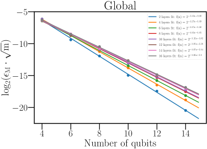
Figure 3: Linear fit of the $\rm{log}_{2}(\epsilon_{\rm M}\cdot\sqrt{m})$ with respect to qubits for the global cost function.

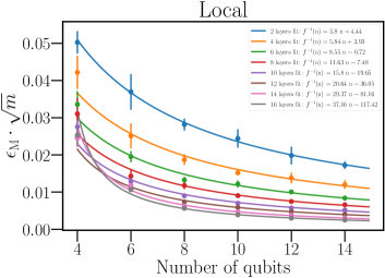
(a)

(b)

Figure 4: Pre-factor scaling fit for the local cost function with the number of qubits. The left panel depicts the linear model results. The right panel corresponds to the quadratic polynomial model. The error bars on the figures are the standard deviation of a sample of 5 independent runs.

(a)

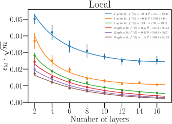
(b)

Figure 5: Pre-factor scaling fit for the local cost function with the number of layers. The left panel depicts the linear model results. The right panel corresponds to the quadratic polynomial model. The error bars on the figures are the standard deviation of a sample of 5 independent runs.

References

- Peruzzo et al. [2014] A. Peruzzo, J. McClean, P. Shadbolt, M.-H. Yung, X.-Q. Zhou, P. J. Love, A. Aspuru-Guzik, and J. L. O’Brien, Nature Communications 5, 4213 (2014).
- Cerezo et al. [2021a] M. Cerezo, A. Arrasmith, R. Babbush, S. C. Benjamin, S. Endo, K. Fujii, J. R. McClean, K. Mitarai, X. Yuan, L. Cincio, and P. J. Coles, Nature Reviews Physics 3, 625 (2021a).
- Bharti et al. [2022] K. Bharti, A. Cervera-Lierta, T. H. Kyaw, T. Haug, S. Alperin-Lea, A. Anand, M. Degroote, H. Heimonen, J. S. Kottmann, T. Menke, W.-K. Mok, S. Sim, L.-C. Kwek, and A. Aspuru-Guzik, Reviews of Modern Physics 94, 015004 (2022).
- Preskill [2018] J. Preskill, Quantum 2, 79 (2018).
- McClean et al. [2018] J. R. McClean, S. Boixo, V. N. Smelyanskiy, R. Babbush, and H. Neven, Nature Communications 9, 4812 (2018).
- Cerezo et al. [2021b] M. Cerezo, A. Sone, T. Volkoff, L. Cincio, and P. J. Coles, Nature Communications 12, 1791 (2021b).
- Wang et al. [2021] S. Wang, E. Fontana, M. Cerezo, K. Sharma, A. Sone, L. Cincio, and P. J. Coles, Nature Communications 12, 6961 (2021).
- Larocca et al. [2022] M. Larocca, P. Czarnik, K. Sharma, G. Muraleedharan, P. J. Coles, and M. Cerezo, Quantum 6, 824 (2022), arxiv:2105.14377 [quant-ph] .
- Herasymenko and O’Brien [2021] Y. Herasymenko and T. E. O’Brien, Quantum 5, 596 (2021).
- Du et al. [2022] Y. Du, Z. Tu, X. Yuan, and D. Tao, Physical Review Letters 128, 080506 (2022).
- Holmes et al. [2022] Z. Holmes, K. Sharma, M. Cerezo, and P. J. Coles, PRX Quantum 3, 010313 (2022).
- Bonet-Monroig et al. [2023] X. Bonet-Monroig, H. Wang, D. Vermetten, B. Senjean, C. Moussa, T. Bäck, V. Dunjko, and T. E. O’Brien, Phys. Rev. A 107, 032407 (2023).
- Nakanishi et al. [2020] K. M. Nakanishi, K. Fujii, and S. Todo, Phys. Rev. Research 2, 043158 (2020).
- Ostaszewski et al. [2021] M. Ostaszewski, E. Grant, and M. Benedetti, Quantum 5, 391 (2021).
- Wilson et al. [2021] M. Wilson, R. Stromswold, F. Wudarski, S. Hadfield, N. M. Tubman, and E. G. Rieffel, Quantum Machine Intelligence 3, 13 (2021).
- Sung et al. [2020] K. J. Sung, J. Yao, M. P. Harrigan, N. C. Rubin, Z. Jiang, L. Lin, R. Babbush, and J. R. McClean, Quantum Science and Technology 5, 044008 (2020).
- Rudolph et al. [2021] M. S. Rudolph, S. Sim, A. Raza, M. Stechly, J. R. McClean, E. R. Anschuetz, L. Serrano, and A. Perdomo-Ortiz, arXiv preprint arXiv:2111.04695 (2021).
- Kerschke and Trautmann [2019] P. Kerschke and H. Trautmann, Evolutionary Computation 27, 99 (2019).
- Zou et al. [2022] F. Zou, D. Chen, H. Liu, S. Cao, X. Ji, and Y. Zhang, Neurocomputing 503, 129 (2022).
- Kerschke et al. [2015] P. Kerschke, M. Preuss, S. Wessing, and H. Trautmann, in Proceedings of the 2015 Annual Conference on Genetic and Evolutionary Computation, GECCO ’15 (Association for Computing Machinery, New York, NY, USA, 2015) p. 265–272.
- Morgan and Gallagher [2017] R. Morgan and M. Gallagher, Soft Comput. 21, 1735 (2017).
- Bischl et al. [2012] B. Bischl, O. Mersmann, H. Trautmann, and M. Preuß, in Proceedings of the 14th Annual Conference on Genetic and Evolutionary Computation, GECCO ’12 (Association for Computing Machinery, New York, NY, USA, 2012) p. 313–320.
- Kostovska et al. [2022] A. Kostovska, A. Jankovic, D. Vermetten, J. de Nobel, H. Wang, T. Eftimov, and C. Doerr, in Parallel Problem Solving from Nature–PPSN XVII: 17th International Conference, PPSN 2022, Dortmund, Germany, September 10–14, 2022, Proceedings, Part I (Springer, 2022) pp. 46–60.
- Muñoz et al. [2015a] M. A. Muñoz, M. Kirley, and S. K. Halgamuge, IEEE Transactions on Evolutionary Computation 19, 74 (2015a).
- Vassilev et al. [2000] V. K. Vassilev, T. C. Fogarty, and J. F. Miller, Evol. Comput. 8, 31–60 (2000).
- Muñoz et al. [2015b] M. A. Muñoz, M. Kirley, and S. K. Halgamuge, IEEE Transactions on Evolutionary Computation 19, 74 (2015b).
- Bailey [1992] R. W. Bailey, The American Statistician 46, 117 (1992), 2684178 .
- Hastings [1970] W. K. Hastings, Biometrika 57, 97 (1970).
- Temme [1992] N. M. Temme, Journal of Computational and Applied Mathematics 41, 145 (1992).
- Tchébychef [1867] P. Tchébychef, Journal de Mathématiques Pures et Appliquées , 177 (1867).
- Pérez-Salinas et al. [2023] A. Pérez-Salinas, H. Wang, and X. Bonet-Monroig, Code and data: Analyzing variational quantum landscapes with information content, Zenodo (2023).
- Johnson et al. [1995] N. L. Johnson, S. Kotz, and N. Balakrishnan, Continuous Univariate Distributions, Volume 2 (John Wiley & Sons, 1995).
- Efthymiou et al. [2022] S. Efthymiou, S. Ramos-Calderer, C. Bravo-Prieto, A. Pérez-Salinas, D. García-Martín, A. Garcia-Saez, J. I. Latorre, and S. Carrazza, Quantum Science and Technology 7, 015018 (2022).
- Kerschke [2017] P. Kerschke, Comprehensive Feature-Based Landscape Analysis of Continuous and Constrained Optimization Problems Using the R-Package flacco (2017), arXiv:1708.05258 .
- Seabold and Perktold [2010] S. Seabold and J. Perktold, in 9th Python in Science Conference (2010).