Are Chebyshev-based stability analysis and Urabe’s error bound useful features for Harmonic Balance?

Abstract

Harmonic Balance is one of the most popular methods for computing periodic solutions of nonlinear dynamical systems. In this work, we address two of its major shortcomings: First, we investigate to what extent the computational burden of stability analysis can be reduced by consistent use of Chebyshev polynomials. Second, we address the problem of a rigorous error bound, which, to the authors’ knowledge, has been ignored in all engineering applications so far. Here, we rely on Urabe’s error bound and, again, use Chebyshev polynomials for the computationally involved operations. We use the error estimate to automatically adjust the harmonic truncation order during numerical continuation, and confront the algorithm with a state-of-the-art adaptive Harmonic Balance implementation. Further, we rigorously prove, for the first time, the existence of some isolated periodic solutions of the forced-damped Duffing oscillator with softening characteristic. We find that the effort for obtaining a rigorous error bound, in its present form, may be too high to be useful for many engineering problems. Based on the results obtained for a sequence of numerical examples, we conclude that Chebyshev-based stability analysis indeed permits a substantial speedup. Like Harmonic Balance itself, however, this method becomes inefficient when an extremely high truncation order is needed as, e.g., in the presence of (sharply regularized) discontinuities.

1 Introduction

Harmonic Balance (HB) is a method for the computation of periodic solutions of nonlinear ordinary and differential-algebraic equation systems. HB is a Fourier-Galerkin method where an approximation is sought in the form of a truncated Fourier series, and the corresponding residual term of the differential equation system is required to be orthogonal to the Fourier base functions contained in the ansatz [1]. The resulting algebraic equation system is commonly solved using a Newton-type method in conjunction with a numerical path continuation technique. To treat generic nonlinearities conveniently within HB, the Alternating Frequency-Time scheme [2] is typically used, where the Fourier coefficients of the nonlinear terms are computed using the discrete Fourier transform. Using HB, the simulation of the possibly long transient is avoided by directly determining the periodic limit state. Near resonance, reasonable accuracy is often achieved already with a few Fourier terms. HB reduces the computational effort often by 2-4 orders of magnitude compared to numerical integration, especially for stiff problems, see [3] (ch. 4.2) and [4] (p. 115). This makes HB a popular method not only in structural dynamics, but also fluid dynamics [5] and electrical circuit analysis [6]. In the following, we place the focus on nonlinear mechanical systems. HB has two major shortcomings, (a) challenges with stability analysis and (b) the lack of an error bound, as detailed in the following two paragraphs.
Throughout this work, asymptotic stability in the sense of Lyapunov is considered. Knowing the asymptotic stability of the computed periodic responses is crucial to distinguish physically feasible from infeasible periodic responses, and to analyze bifurcations. Two fundamentally different approaches are known for analyzing the asymptotic stability of HB approximations, the monodromy matrix method and Hill’s method. For the former, the differential equation is linearized around the approximated periodic orbit, and the fundamental matrix associated with this linearized problem is computed [7, 8]. The monodromy matrix is the fundamental matrix evaluated at the end of one period. According to the Floquet theorem, the orbit is asymptotically stable if all eigenvalues of this matrix (Floquet multipliers) lie within the unit disk in the complex plane. The main task is here to compute the monodromy matrix, which is commonly achieved by numerical time step integration. Different integration methods can be used, and many of these have been compared by Peletan et al. [9]. They found that the Newmark Method (constant-average-acceleration variant) performed best among the selected set of methods. In contrast to the monodromy matrix method, Hill’s method is formulated entirely in the frequency domain (no time integration needed) [10]. Essentially, this yields a quadratic eigenvalue problem of dimension $d(2H+1)$ where $d$ is the number of degrees of freedom and $H$ is the harmonic truncation order. The coefficient matrices of this eigenvalue problem are usually readily available from the solution of the HB equations. The corresponding eigenvalues should be directly related to the Floquet multipliers. Due to the finite truncation order in practice, however, some of the eigenvalues are more accurately approximated than others [11]. Hence, there is a consensus that the eigenspectrum must be filtered for the most accurate ones, but there is no consensus on how to do that [12, 11]. It is known that with all currently available filter methods, Hill’s method still gives erroneous results in some cases [9, 4]; hence, Hill’s method is not further considered in the present work.
As stated above, besides the problems with stability analysis, HB has another major limitation: almost nothing is known on the error of the HB approximation. When no error bound can be given, the existence of an exact periodic solution in the neighborhood of a HB approximation is not guaranteed. Indeed, there are simple and frequently-studied examples, such as the Duffing oscillator with softening characteristic, where low-order HB suggests periodic response regimes that turn out not to exist [13]. Several authors have proposed to use some norm of the time-domain residual, which is obtained when the HB approximation is substituted back into the initial differential equation system, as error indicator, see e. g. [13, 14, 15]. It was proposed to use such residual norms to define rules for automatically adjusting the harmonic truncation order (adaptive HB [15, 16]). An alternative to using the residual itself (effectively: violation of the dynamic force balance) as error indicator, is to compute and use the linear response to the non-balanced higher harmonics of the nonlinear forces [17, 15]. The underlying assumption of both error indicators is a good correlation between the time-domain residual and the error (deviation between exact response and HB approximation). However, there is only a poor correlation in some cases, as shown e. g. for a system with dry friction nonlinearity in [17]. It is remarkable that a mathematically rigorous a posteriori error bound was already developed 1965 by Urabe [1]. However, this was so far only applied by Urabe himself [1, 19] and by van Dooren [20], and only to single-degree-of-freedom oscillators with cubic nonlinear terms. It should be remarked that alternative a posteriori methods for rigorously obtaining an error bound have been proposed, for instance those proposed by Baker et al. [21], and Lessard et al. [22, 23]. An advantage of the approach in [21] is that it requires only continuity of the vector field, whereas continuous differentiability is required in [1, 22, 23]. A drawback of that approach is that homology computations are explicitly required, which is expected to yield higher computation effort. The approach in [22, 23] is not expected to differ substantially in terms of computation effort compared to Urabe’s approach. However, in the authors’ opinion, Urabe’s approach has the important benefit that it can be rather easily implemented in such a way that it is applicable to quite generic nonlinearities. Thus, only Urabe’s error bound [1] is investigated in the present work. Further, it is noteworthy that first steps towards a priori error estimation were done in [24]. The method is still limited to systems with linear viscous damping, and will not further be considered in this work.
The purpose of the present work is to address the above mentioned two major shortcomings of HB. More specifically, we seek to analyze to what extent the properties of Chebyshev polynomials can be exploited to speed up the computation of the monodromy matrix and thus the stability analysis of nonlinear dynamical systems. In particular, product and integration properties of Chebyshev polynomials permit to transform the ordinary differential equation system governing the monodromy matrix into an algebraic equation system, and thus to avoid time step integration. In addition, Chebyshev polynomials show superior convergence behavior when approximating continuous functions [25]. Further, we aim to determine the engineering value of a rigorous a posteriori error estimation for the first time. For this, we will focus on Urabe’s error bound [1]. In this work, we will present an approach for its computational evaluation and apply it towards engineering relevant problems. In Section 2, the HB method, the state-of-the-art methods for stability analysis as well as the proposed Chebyshev-based method are presented. In Section 3, Urabe’s error bound is explained and a computational scheme for its evaluation is proposed. Subsequently, the numerical performance of the Chebyshev-based stability analysis and the error bound are assessed for representative examples in Section 4 and Section 5, respectively. This article ends with concluding remarks in Section 6.

2 Harmonic Balance and stability analysis

In the following, we define the equation of motion considered throughout this work. Then, a brief recap of Harmonic Balance (HB) is given, including its popular implementation using the Alternating Frequency-Time scheme. Then the problem of analyzing the asymptotic stability of the found periodic oscillation is formulated. Finally, computational methods for stability analysis are presented, including two of the most popular methods, and the aforementioned original method based on Chebyshev polynomials.

2.1 Problem setting

Consider nonlinear mechanical systems described by the equation of motion

$$\Omega^{2}{\boldsymbol{q}}^{\prime\prime}+\Omega\boldsymbol{D}{\boldsymbol{q}}^{\prime}+\boldsymbol{K}\boldsymbol{q}+\boldsymbol{f}_{\mathrm{nl}}(\boldsymbol{q})-\boldsymbol{f}_{\mathrm{ex}}(\tau)=\boldsymbol{0}\,,$$ (1)

where $\boldsymbol{q}\in\mathbb{R}^{d\times 1}$ is the vector of $d$ generalized coordinates, $\square^{\prime}$ denotes derivative with respect to normalized time $\tau$, which is related to the non-normalized time $t$ via $\tau=\Omega t$. The external force is $2\pi$-periodic, $\boldsymbol{f}_{\mathrm{ex}}(\tau+2\pi)=\boldsymbol{f}_{\mathrm{ex}}(\tau)$. The vector of nonlinear forces, $\boldsymbol{f}_{\mathrm{nl}}$, depends only on $\boldsymbol{q}$. The coefficient matrices $\boldsymbol{D},\boldsymbol{K}\in\mathbb{R}^{d\times d}$ are time-invariant. The models considered throughout the numerical examples are all of the form in Eq. (1). The following formulations can be generalized, among others, to $\boldsymbol{q}^{\prime}$-dependent and explicitly time-dependent nonlinear forces, non-trivial coefficient matrices of vector ${\boldsymbol{q}}^{\prime\prime}$, and time-periodic coefficient matrices for different derivative orders. For convergence of HB, the applicability of Urabe’s error bound and the Floquet theorem, sufficient differentiability of $\boldsymbol{f}_{\mathrm{nl}}$ and $\boldsymbol{f}_{\mathrm{ex}}$ with respect to $\boldsymbol{q}$ and $\tau$, respectively, must be required [1] (lemma 2.2). The numerical examples are restricted to analytic functions (infinitely differentiable).

2.2 Harmonic Balance

HB approximates $\boldsymbol{q}(\tau)$ as Fourier series, $\boldsymbol{q}(\tau)\approx\boldsymbol{q}_{H}(\tau)$, truncated to order $H$,

$$\boldsymbol{q}_{H}(\tau)=\sum_{k=-H}^{H}\hat{\boldsymbol{q}}(k)\mathrm{e}^{\mathrm{i}k\tau}\,,$$ (2)

which is written here in complex-exponential form with the imaginary unit $\mathrm{i}=\sqrt{-1}$. To ensure that $\boldsymbol{q}_{H}(\tau)$ is real-valued, the Fourier coefficients are pairwise complex-conjugate, $\hat{\boldsymbol{q}}(-k)=\overline{\hat{\boldsymbol{q}}}(k)$, where $\overline{\square}$ denotes complex-conjugate. HB requires that the Fourier coefficients of the residual obtained by substituting Eq. (2) into Eq. (1) vanish with regard to the retained harmonics (up to order $H$). This corresponds to a Fourier-Galerkin projection and can be expressed as algebraic equation system

$$\left(-k\Omega^{2}+\mathrm{i}k\Omega\boldsymbol{D}+\boldsymbol{K}\right)\hat{\boldsymbol{q}}(k)+\hat{\boldsymbol{f}}_{\mathrm{nl}}(k)-\hat{\boldsymbol{f}}_{\mathrm{ex}}(k)=\boldsymbol{0}\quad k=-H,\ldots,H\,.$$ (3)

As already proposed by Urabe and Reiter [19], the Fourier coefficients can be computed via discrete Fourier transform, e. g.

$$\hat{\boldsymbol{f}}_{\mathrm{nl}}(k)=\frac{1}{N_{\mathrm{AFT}}}\sum_{n=0}^{N_{\mathrm{AFT}}-1}\boldsymbol{f}_{\mathrm{nl}}\left(\boldsymbol{q}_{H}\left(\tau_{n}\right)\right)\mathrm{e}^{-\mathrm{i}k\tau_{n}}\quad\tau_{n}=\frac{2\pi}{N_{\mathrm{AFT}}}n\quad k=-H,\ldots,H\,.$$ (4)

This approach is now well-known as Alternating Frequency-Time scheme [2] and is the most popular approach for evaluating the Fourier coefficients of the nonlinear terms, both for polynomial and generic nonlinearities [4] (ch. 2.4). It is common to solve the algebraic equation system in Eq. (3) with respect to the unknown Fourier coefficients of $\boldsymbol{q}_{H}$ using a Newton-type method in conjunction with analytical gradients, and to combine this technique with predictor-corrector path continuation [4] (ch. 4.4).

2.3 Stability according to Floquet theory

Once a periodic oscillation, $\boldsymbol{q}_{\mathrm{p}}(\tau+2\pi)=\boldsymbol{q}_{\mathrm{p}}(\tau)$ is known (or its approximation $\boldsymbol{q}_{H}(\tau)$), the Floquet theorem is commonly used to analyze its asymptotic stability. The idea is to consider an infinitesimal perturbation, $\Delta\boldsymbol{q}$, around $\boldsymbol{q}_{\mathrm{p}}$ and determine whether this grows over a period. The mapping over one period is given by the monodromy matrix, which is the fundamental matrix, $\boldsymbol{\Phi}(\tau)$, evaluated at the end of the period, $\boldsymbol{\Phi}(2\pi)$. If all eigenvalues of the monodromy matrix (Floquet multipliers) are within the unit disk in the complex plane, $\boldsymbol{q}_{\mathrm{p}}$ is asymptotically stable; if there is at least one eigenvalue outside the unit disk, the periodic oscillation is unstable. By the way the Floquet multipliers cross the unit circle, the type of bifurcation can be inferred. By linearizing Eq. (1) for $\boldsymbol{q}=\boldsymbol{q}_{\mathrm{p}}+\Delta\boldsymbol{q}$ around $\boldsymbol{q}_{\mathrm{p}}$, one obtains a linear ordinary differential equation for $\Delta\boldsymbol{q}$,

$$\Omega^{2}\Delta\boldsymbol{q}^{\prime\prime}+\Omega\boldsymbol{D}\Delta\boldsymbol{q}^{\prime}+\boldsymbol{K}\Delta\boldsymbol{q}+\underbrace{\left.\frac{\partial\boldsymbol{f}_{\mathrm{nl}}}{\partial\boldsymbol{q}}\right|_{\boldsymbol{q}_{\mathrm{p}}}}_{\boldsymbol{J}\left(\boldsymbol{q}_{\mathrm{p}}\left(\tau\right)\right)}\Delta\boldsymbol{q}=\boldsymbol{0}\,,$$ (5)

where $\boldsymbol{J}$ is the Jacobian. It is useful to cast Eq. (1) in state-space form,

$$\boldsymbol{x}=\left[\!\!\begin{array}[]{c}\boldsymbol{q}\\ \boldsymbol{u}\end{array}\!\!\right]\quad\boldsymbol{x}^{\prime}=\left[\!\!\begin{array}[]{c}\boldsymbol{u}\\ \boldsymbol{f}_{\mathrm{ex}}(\tau)-\frac{1}{\Omega^{2}}\left(\Omega\boldsymbol{D}\boldsymbol{u}+\boldsymbol{K}\boldsymbol{q}+\boldsymbol{f}_{\mathrm{nl}}(\boldsymbol{q})\right)\end{array}\!\!\right]=\boldsymbol{F}\left(\boldsymbol{x},\tau\right)\,.$$ (10)

The fundamental matrix $\boldsymbol{\Phi}$ contains as columns the solution of Eq. (5) for unit initial conditions. This can be compactly written as matrix initial value problem,

$$\boldsymbol{\Phi}^{\prime}=\underbrace{\left[\!\!\begin{array}[]{cc}\boldsymbol{0}&\boldsymbol{I}\\ -\frac{1}{\Omega^{2}}\left(\boldsymbol{K}+\boldsymbol{J}\left(\boldsymbol{q}_{\mathrm{p}}\left(\tau\right)\right)\right)\qquad-\frac{1}{\Omega}\boldsymbol{D}\end{array}\!\!\right]}_{\boldsymbol{A}\left(\boldsymbol{x}_{\mathrm{p}}\left(\tau\right)\right)}\boldsymbol{\Phi}\quad\boldsymbol{\Phi}(0)=\boldsymbol{I}\,,$$ (13)

where $\boldsymbol{x}_{\mathrm{p}}(\tau)$ is the $2\pi$-periodic state space representation of the periodic oscillation, and $\boldsymbol{I}$ denotes identity matrices of according dimension.

2.4 Computational stability analysis

Three different methods for computing the monodromy matrix $\boldsymbol{\Phi}(2\pi)$ are outlined in the following, the Matrix Exponential Method (MExp), the Newmark Method (NTP) and the Chebyshev Method (Cheby). While the first two methods are commonly applied, the last one has never been used for analyzing the stability of periodic oscillations of nonlinear mechanical systems. Chebyshev polynomials have, however, been proposed for computing monodromy matrices of linear mechanical systems with time-periodic coefficient matrices [26, 27].

2.4.1 Matrix Exponential Method (MExp)

The Matrix Exponential Method simply approximates the matrix $\boldsymbol{A}$ in Eq. (13) as piecewise constant between two time levels. The only time-varying part of $\boldsymbol{A}$ is $\boldsymbol{J}$. An expression for $\boldsymbol{J}$ is commonly available, as this is an auxiliary variable when evaluating analytical gradients (typically used in conjunction with Newton-type methods for solving the HB equations). For $\boldsymbol{A}(\tau)\approx\boldsymbol{A}(\tau_{n})$ within $\tau_{n}\leq\tau\leq\tau_{n+1}$, it holds that $\boldsymbol{\Phi}(\tau_{n+1})=\mathrm{e}^{\boldsymbol{A}(\tau_{n})~{}\left(\tau_{n+1}-\tau_{n}\right)}\boldsymbol{\Phi}(\tau_{n})$, where $\mathrm{e}^{\square}$ denotes the matrix exponential. Here and in the following, we write $\boldsymbol{A}(\tau)$ and $\boldsymbol{J}(\tau)$ short hand for $\boldsymbol{A}\left(\boldsymbol{x}_{\mathrm{p}}\left(\tau\right)\right)$ and $\boldsymbol{J}\left(\boldsymbol{q}_{\mathrm{p}}\left(\tau\right)\right)$, respectively. Applying this on a regular grid,

$$\tau_{1}=0\,,\tau_{N+1}=2\pi\,,\tau_{n+1}-\tau_{n}=2\pi/N\,,$$ (14)

yields

$$\boldsymbol{\Phi}(2\pi)=\prod_{n=1}^{N}\mathrm{e}^{\boldsymbol{A}(\tau_{n})\frac{2\pi}{N}}\,.$$ (15)

The product in Eq. (15) is to be carried out as successive multiplication from the left.
It seems tempting to use the grid points from the discrete Fourier transform in Eq. (4), and simply set $N=N_{\mathrm{AFT}}$. This is because $\boldsymbol{J}$ is readily available upon solution of the HB equations, as mentioned above. However, it turns out that commonly a much finer temporal resolution is needed for stability analysis. For a cubic-order nonlinearity, for instance, a number of $N_{\mathrm{AFT}}=4H+1$ samples is sufficient to avoid aliasing within the Alternating Frequency-Time scheme [28] (appx. A), whereas one to two orders of magnitude more time steps may be required to achieve reasonable accuracy of the Floquet multipliers, as will be shown later. In practice, therefore, $\boldsymbol{J}$ has to be evaluated on a finer grid with $N>N_{\mathrm{AFT}}$. This applies also to the method subsequently described.

2.4.2 Newmark Method (NTP)

The Newmark Method for computing the monodromy matrix directly uses Eq. (5) as point of departure. More specifically, the constant-average-acceleration variant is used for numerical integration. Again, the grid defined in Eq. (14) is used with the constant (normalized) time step $2\pi/N$. This leads to the scheme:

$$\boldsymbol{S}_{n+1}\boldsymbol{\Delta}\boldsymbol{q}_{n+1} =\boldsymbol{b}_{n+1}\,,$$ (16)

$$\Delta\boldsymbol{u}_{n+1} =\frac{N}{\pi}\left(\Delta\boldsymbol{q}_{n+1}-\Delta\boldsymbol{q}_{n}\right)-\Delta\boldsymbol{u}_{n}\,,$$ (17)

$$\Delta\boldsymbol{u}^{\prime}_{n+1} =\frac{N^{2}}{\pi^{2}}\left(\Delta\boldsymbol{q}_{n+1}-\Delta\boldsymbol{q}_{n}\right)-\frac{2N}{\pi}\Delta\boldsymbol{u}_{n}-\Delta\boldsymbol{u}^{\prime}_{n}\,,$$ (18)

$$\text{with}~{}~{}\boldsymbol{S}_{n+1} =\left(\frac{N\Omega}{\pi}\right)^{2}\boldsymbol{I}+\frac{N\Omega}{\pi}\boldsymbol{D}+\boldsymbol{K}+\boldsymbol{J}\left(\tau_{n+1}\right)\,,$$ (19)

$$\boldsymbol{b}_{n+1} =\Omega^{2}\left(\frac{N^{2}}{\pi^{2}}\Delta\boldsymbol{q}_{n}+\frac{2N}{\pi}\Delta\boldsymbol{u}_{n}+\Delta\boldsymbol{u}^{\prime}_{n}\right)+\Omega\boldsymbol{D}\left(\frac{N}{\pi}\Delta\boldsymbol{q}_{n}+\Delta\boldsymbol{u}_{n}\right)\,.$$ (20)

As in Eq. (13), the scheme is applied in matrix form to the set of unit initial values, $\Delta\boldsymbol{q}_{1}=\left[\!\!\begin{array}[]{cc}\boldsymbol{I}&\boldsymbol{0}\end{array}\!\!\right]$, $\Delta\boldsymbol{u}_{1}=\left[\!\!\begin{array}[]{cc}\boldsymbol{0}&\boldsymbol{I}\end{array}\!\!\right]$ which are each of dimension $d\times 2d$. To evaluate Eq. (16) at $n=1$, $\Delta\boldsymbol{u}^{\prime}_{1}=\Delta\boldsymbol{q}^{\prime\prime}_{1}$ is required, which is obtained with the initial values and $\boldsymbol{J}\left(\tau_{1}\right)$ from Eq. (5). The scheme in Eqs. (16)-(18) is then applied for $n=1,\ldots,N$, to obtain $\boldsymbol{\Phi}(2\pi)=[\Delta\boldsymbol{q}_{N+1};\Delta\boldsymbol{u}_{N+1}]$.

2.4.3 Chebyshev Method (Cheby)

The idea of the Chebyshev Method is to seek an approximate solution of Eq. (5) in the form of a Chebyshev polynomial. One should recall that although the considered oscillation, $\boldsymbol{q}_{\mathrm{p}}$, is $2\pi$-periodic, and hence Eq. (13) has a $2\pi$-periodic coefficient matrix, the sought matrix, $\boldsymbol{\Phi}(\tau)$, is, of course, not periodic. Consequently, it is not possible to approximate $\boldsymbol{\Phi}(\tau)$ as a Fourier polynomial, but one has to resort to more generic polynomials such as the Chebyshev polynomials. Chebyshev polynomials have many favorable properties, including the ability to express integration and multiplication using operational matrices, cf.  A. This permits to derive a linear algebraic equation system for the sought Chebyshev coefficients. In this work, we use Chebyshev base functions of the first kind, $T_{j}(\tau)$, which are shifted from the standard interval $[-1,1]$ to the interval $\tau\in[0,2\pi]$. Let us define $a_{C}(\tau)$ as Chebyshev polynomial,

$$a_{C}(\tau)=\sum_{j=1}^{C}T_{j}(\tau)\check{a}(j)\quad\tau\in[0,2\pi]\,,$$ (21)

with the truncation order $C$ and the Chebyshev coefficients $\check{a}(j)$. For compact notation, the coefficients are collected in a vector $\check{\boldsymbol{a}}=[\check{a}(1);\ldots;\check{a}(C)]$.
In the following, we derive a linear algebraic equation system for the Chebyshev coefficients of the sought approximation. To make use of the integration rule, one first has to integrate Eq. (5) two times, in the interval from $0$ to $\tau$,

$$\Omega^{2}\left(\Delta\boldsymbol{q}^{\prime}\left(\tau\right)-\Delta\boldsymbol{q}^{\prime}\left(0\right)\right)+\Omega\boldsymbol{D}\left(\Delta\boldsymbol{q}\left(\tau\right)-\Delta\boldsymbol{q}\left(0\right)\right)+\int_{0}^{\tau}\left(\boldsymbol{K}+\boldsymbol{J}\left(\tau^{\bullet}\right)\right)\Delta\boldsymbol{q}\left(\tau^{\bullet}\right)\mathrm{d}\tau^{\bullet}=\boldsymbol{0} \,,$$ (22)

$$\begin{split}\Omega^{2}\left(\Delta\boldsymbol{q}\left(\tau\right)-\Delta\boldsymbol{q}\left(0\right)-\int_{0}^{\tau}\Delta\boldsymbol{q}^{\prime}\left(0\right)\mathrm{d}\tau^{\circ}\right)+\Omega\boldsymbol{D}\int_{0}^{\tau}\Delta\boldsymbol{q}\left(\tau^{\circ}\right)-\Delta\boldsymbol{q}\left(0\right)\mathrm{d}\tau^{\circ}&\\ +\int_{0}^{\tau}\int_{0}^{\tau^{\circ}}\left(\boldsymbol{K}+\boldsymbol{J}\left(\tau^{\bullet}\right)\right)\Delta\boldsymbol{q}\left(\tau^{\bullet}\right)\mathrm{d}\tau^{\bullet}\mathrm{d}\tau^{\circ}=\boldsymbol{0}&\,.\end{split}$$ (23)

Herein, some integrals are trivial because the integrand is constant; the notation as integral has the advantage that the expression can be conveniently cast into Chebyshev space (via the integration rule). As outlined in A, integration is carried out using the operational matrix $\boldsymbol{G}$ in Chebyshev space. Further, the time-dependent matrix $\boldsymbol{J}(\tau)$ is represented as Chebyshev polynomial, by applying the discrete Chebyshev transform described below. Then the product of $\boldsymbol{J}(\tau^{\bullet})\Delta\boldsymbol{q}(\tau^{\bullet})$ in Eq. (23) can be carried out in Chebyshev space using the product operational matrix also defined in A. With this, the representation of Eq. (23) in Chebyshev space reads:

$$\boldsymbol{C}\Delta\check{\boldsymbol{q}} =\boldsymbol{c}\,,$$ (24)

$$\boldsymbol{C} =\Omega^{2}\boldsymbol{I}+\Omega\boldsymbol{D}\otimes\boldsymbol{G}^{\mathrm{T}}+\boldsymbol{K}\otimes\left(\boldsymbol{G}^{\mathrm{T}}\right)^{2}+\left(\boldsymbol{I}\otimes\left(\boldsymbol{G}^{\mathrm{T}}\right)^{2}\right)\boldsymbol{P}\left(\check{\boldsymbol{J}}\right)\,,$$ (25)

$$\boldsymbol{c} =\left(\Omega^{2}\boldsymbol{I}+\Omega\boldsymbol{D}\otimes\boldsymbol{G}^{\mathrm{T}}\right)\Delta\check{\boldsymbol{q}}\left(0\right)+\Omega^{2}\left(\boldsymbol{I}\otimes\boldsymbol{G}^{\mathrm{T}}\right)\Delta\check{\boldsymbol{q}}^{\prime}\left(0\right)\,.$$ (26)

Eq. (24) is a linear algebraic equation system for the sought Chebyshev coefficients of the perturbation $\Delta\boldsymbol{q}$, for given initial conditions $\Delta\boldsymbol{q}(0)$, $\Delta\boldsymbol{q}^{\prime}(0)$. The Chebyshev coefficients of the (time-constant) initial conditions in Eq. (26), $\Delta\check{\boldsymbol{q}}\left(0\right)$ and $\Delta\check{\boldsymbol{q}}^{\prime}\left(0\right)$, are trivial. Analogous to the Matrix Exponential and the Newmark Method, Eq. (24) is applied in matrix form to the complete set of $2d$ unit initial values. This way, the Chebyshev coefficients of the fundamental matrix $\boldsymbol{\Phi}(\tau)$ are obtained. The square coefficient matrix $\boldsymbol{C}$ has dimension $Cd$.
To evaluate Eq. (25), $\boldsymbol{J}(\tau)$ must be approximated as Chebyshev polynomial, which is to be achieved using a discrete Chebyshev transform. As with the Matrix Exponential and Newmark Methods, $\boldsymbol{J}$ generally has to be re-evaluated on a finer grid. In the case of the Chebyshev Method, it turns out that an equidistant grid leads to poor convergence due to the Runge phenomenon. To overcome this problem, it is proposed to use a non-equidistant grid,

$$\tilde{\tau}_{n}=\pi\left(1-\cos\left(\frac{n-\frac{1}{2}}{C}\pi\right)\right)\quad n=\frac{1}{2},2,3,\ldots,C-1,C+\frac{1}{2}\,.$$ (27)

This way, the grid becomes denser towards the interval limits according to the roots of the Chebyshev polynomials. Using $n=1/2$ instead of $n=1$, and $n=C+1/2$ instead of $n=C$ ensures that the interval limits $0$ and $2\pi$ are contained. Fig. 1 illustrates the superior convergence behavior achieved with the proposed non-equidistant grid, compared to the case of an equidistant grid. The interpolated functions are elements of the matrix $\boldsymbol{J}$ obtained for a cubic nonlinearity (a) and a regularized unilateral spring (b), cf.  Section 4. For both functions (a) and (b), the equidistant grid leads to severe numerical oscillations near the interval boundaries. When the proposed non-equidistant grid is used, in contrast, inevitable numerical oscillations occur only near the (regularized) discontinuity.

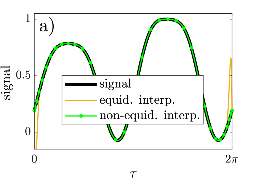
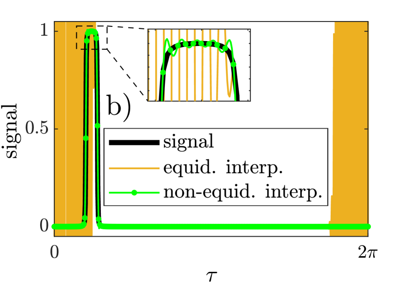
Figure 1: Interpolation of time-periodic functions with Chebyshev polynomials using equidistant vs. non-equidistant grids: (a) function originating from the ECL benchmark (cubic nonlinearity; $C=35$); (b) function originating from oscillator with regularized unilateral spring nonlinearity ($C=300$)

Besides the superior convergence, the particular choice of the non-equidistant grid has the advantage that the Chebyshev polynomials are easy to evaluate. More specifically, it is not necessary to use the recurrence definition, but one simply has $T_{j}(\tilde{\tau}_{n})=\cos\left(j\left(\frac{n-\frac{1}{2}}{C}-1\right)\pi\right)$. For the polynomial defined in Eq. (21), the discrete transform can be compactly written as

$$\tilde{\boldsymbol{a}}=\tilde{\boldsymbol{T}}\check{\boldsymbol{a}}\,,$$ (28)

with $\tilde{\boldsymbol{a}}=[a(\tilde{\tau}_{\frac{1}{2}});\ldots;a(\tilde{\tau}_{C+\frac{1}{2}})]$ and $\boldsymbol{T}=[t_{nj}]=[T_{j}(\tilde{\tau}_{n})]\in\mathbb{R}^{C\times C}$. To obtain Chebyshev coefficients of $\boldsymbol{J}$, one first has to re-evaluate $\boldsymbol{J}$ on the non-equidistant grid, and then the inverse of $\tilde{\boldsymbol{T}}$ is used to solve Eq. (28) for the Chebyshev coefficients. Note that the re-evaluation of $\boldsymbol{J}$ is not an important drawback of the Chebyshev Method, as such a re-evaluation is typically needed for the other methods as well, in order to achieve reasonable accuracy.

3 Urabe’s error bound and its computational implementation

Urabe [1] established a sufficient condition for the existence of an exact periodic solution in the $\delta$-neighborhood,

$$||\boldsymbol{x}_{\mathrm{exact}}-\boldsymbol{x}_{H}||<\delta\,,$$ (29)

of the $H$-order HB approximation $\boldsymbol{x}_{H}$. Here, we use the state space representation introduced in Eq. (10). The condition relies on three scalar measures, an upper bound $r$ of the time-domain residual, an upper bound $\Delta$ of the variation of the Jacobian, and an upper bound $M$ for the propagation of errors within the dynamical system. These measures are defined below and it is explained how they can be computed. Subsequently, Urabe’s existence condition is specified and the relation between $\delta$ and $r,\Delta,M$ is given.
An upper bound $r$ of the time-domain residual, $\dot{\boldsymbol{x}}_{H}(\tau)-\boldsymbol{F}(\boldsymbol{x}_{H}(\tau),\tau)$, is given by:

$$||\dot{\boldsymbol{x}}_{H}(\tau)-\boldsymbol{F}(\boldsymbol{x}_{H}(\tau),\tau)||\leq||\sum\limits_{k=0}^{\infty}||\hat{\boldsymbol{r}}(k)||=||\sum\limits_{k=0}^{H}||\hat{\boldsymbol{r}}(k)||+\sum\limits_{k=H+1}^{\infty}||\hat{\boldsymbol{r}}(k)||=r\,.$$ (30)

Herein, $||\cdot||$ denotes the Euclidian norm and $\hat{\boldsymbol{r}}(k)$ are the Fourier coefficients of the time-domain residual. To determine $r$ conveniently, it is split into two parts, one associated with all harmonics up to order $H$ and one associated with higher orders. HB requires the first part to vanish. However, in computational practice, there is a non-zero residual, controlled by the numerical tolerance of the Newton-type solver. This part is therefore readily available upon numerical solution of the HB equations. As linear terms in Eq. (1) do not generate any higher harmonics, the higher harmonic part of $r$ is only due to the nonlinear forces $\boldsymbol{f}_{\mathrm{nl}}$. The higher harmonics of the nonlinear forces, generated by the HB approximation, can be computed within the Alternating Frequency-Time scheme. For polynomial nonlinearities, one can exploit that the order of the highest harmonic is finite and can be easily determined. For non-polynomial ones, an infinite number of higher harmonics is usually generated. Here, a reasonable finite truncation order $H^{+}\gg H$ has to be selected in practice.
$\Delta(\delta)$ is an upper bound of the variation of the matrix $\boldsymbol{A}=\partial\boldsymbol{F}/\partial\boldsymbol{x}$, defined in Eq. (13),

$$\Delta(\delta){\leq}\max_{\tau}\left|\left|~{}\left.\boldsymbol{A}(\boldsymbol{x})\right|_{\boldsymbol{x}_{\mathrm{exact}}(\tau)}~{}-~{}\left.\boldsymbol{A}(\boldsymbol{x})\right|_{\boldsymbol{x}_{H}(\tau)}~{}\right|\right|,$$ (31)

within the $\delta$-neighborhood of $\boldsymbol{x}_{H}$ given by Eq. (29). Since the linear forces only yield a constant part of $\boldsymbol{A}$, they do not contribute to $\Delta$, so only the nonlinear forces must be considered. An analytical expression of the Jacobian $\boldsymbol{J}$ of the nonlinear forces is established within the Alternating Frequency-Time scheme, as explained earlier. The variation is subsequently determined analytically for each nonlinearity individually and then accumulated to determine the Frobenius norm.
The third and last scalar measure required for Urabe’s theorem, $M$, can be interpreted as a measure for the error propagation over one cycle. It is defined as,

$${M}= \sqrt{{2\pi}\cdot\underset{\tau}{\mathrm{max}}\left(\int\limits_{0}^{{2\pi}}\sum\limits_{k,l}H_{kl}^{2}(\tau,s)\mathrm{d}s\right)}\,,$$ (32)

where the matrix $\boldsymbol{H}=[H_{kl}]$ is given as the piecewise continuous function of the fundamental matrix $\boldsymbol{\Phi}$,

$$\boldsymbol{H}(\tau,s)=\begin{cases}\boldsymbol{\Phi}(\tau)\left[\boldsymbol{I}-\boldsymbol{\Phi}(2\pi)\right]^{-1}\boldsymbol{\Phi}^{-1}(s)&\text{for}\quad 0\leq s\leq\tau\leq 2\pi\\ \boldsymbol{\Phi}(\tau)\left[\boldsymbol{I}-\boldsymbol{\Phi}(2\pi)\right]^{-1}\boldsymbol{\Phi}(2\pi)\boldsymbol{\Phi}^{-1}(s)&\text{for}\quad 0\leq\tau\leq s\leq 2\pi\end{cases}\,.$$ (33)

Urabe’s theorem requires continuous differentiability of $\boldsymbol{F}(\boldsymbol{x},\tau)$ and its first-order derivative in both arguments, which ensures convergence of $M$ with increasing resolution in $\tau$. Clearly, $M$ is computationally much more expensive to determine than $r$ or $\Delta$. To reduce the computational burden, again, consistent use is made of the properties of Chebyshev polynomials. From the stability analysis, the fundamental matrix $\boldsymbol{\Phi}(\tau$) is readily available as Chebyshev polynomial. The multiplication and integration rules are used to first determine the matrix $\boldsymbol{H}$ and then to carry out multiplication and integration in Eq. (32). Recently, it was proposed to reduce the effort for computing $M$ by using an upper bound based on the leading Floquet multipliers [29]. As we shall see later, a more conservative bound for $M$ will generally necessitate higher truncation orders, from which on a finite error bound can be given. Indeed, we shall see that rather high truncation orders are necessary already with Urabe’s approach, which is why the variant proposed in [29] was not further pursued in the present work.

Figure 2: Graphical illustration of Urabe’s theorem.

Based on the three measures, $r$, $\Delta$, $M$, Urabe formulated the following theorem: If there is a non-negative $\kappa<1$ and a positive $\delta$ so that,

$$\Delta(\delta)M\leq\kappa\quad\mathrm{and}\quad\kappa\leq 1-Mr/\delta,$$ (34)

then there exists one and only one periodic solution within the defined $\delta$-neighborhood. For the considered simple examples (single-DOF oscillators with cubic nonlinearity), Urabe and Reiter [19] treated these inequalities analytically, in an individual way for each example. In this work, an approach is pursued that can be more easily automatized: From the above theorem, one can identify $M\Delta(\delta)$ as lower bound, and $1-Mr/\delta$ as upper bound for $\kappa$. This is illustrated in Fig. 2. One can identify the admissible range for $\kappa$ and $\delta$ in accordance with Urabe’s requirement. Obviously, the lowest $\delta$ represents the tightest error bound. In the following, we refer to the tightest error bound simply by $\delta$. One can also see that for sufficiently large $M$ or $r$, no intersection point will occur. In this case, no error bound for the HB approximation can be given (and hence the existence of a periodic solution is not guaranteed). Thereby, the stronger the repelling nature of the cycle, i. e. the further at least one of the Floquet multipliers lies outside the unit circle, the larger the magnitude of $M$ becomes. For large $M$, $r$ must be sufficiently small so that the error estimation can be successful. Thus, the success of the procedure can change by further increasing the truncation order $H$, as $r$ may be reduced substantially. This way, at best, one may prove the existence of a periodic solution (and give an error bound). However, it is impossible to prove the non-existence of a periodic solution in this way.

4 Numerical results: Chebyshev-based stability analysis

Two numerical examples are considered in this section, the ECL benchmark involving an (inherently smooth) cubic-order stiffness nonlinearity, and a two-degree-of-freedom oscillator with a regularized elastic stop. To this end, the methods described in Subsection 2.4 and Section 3 have been implemented in MATLAB, using the open-source MATLAB tool NLvib [4] (appx. C) as point of departure.

4.1 ECL benchmark

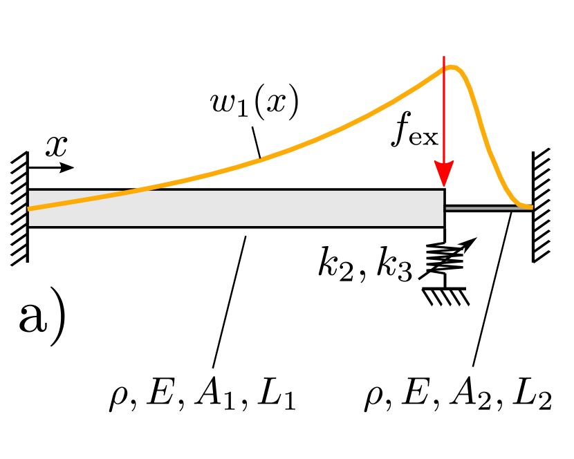
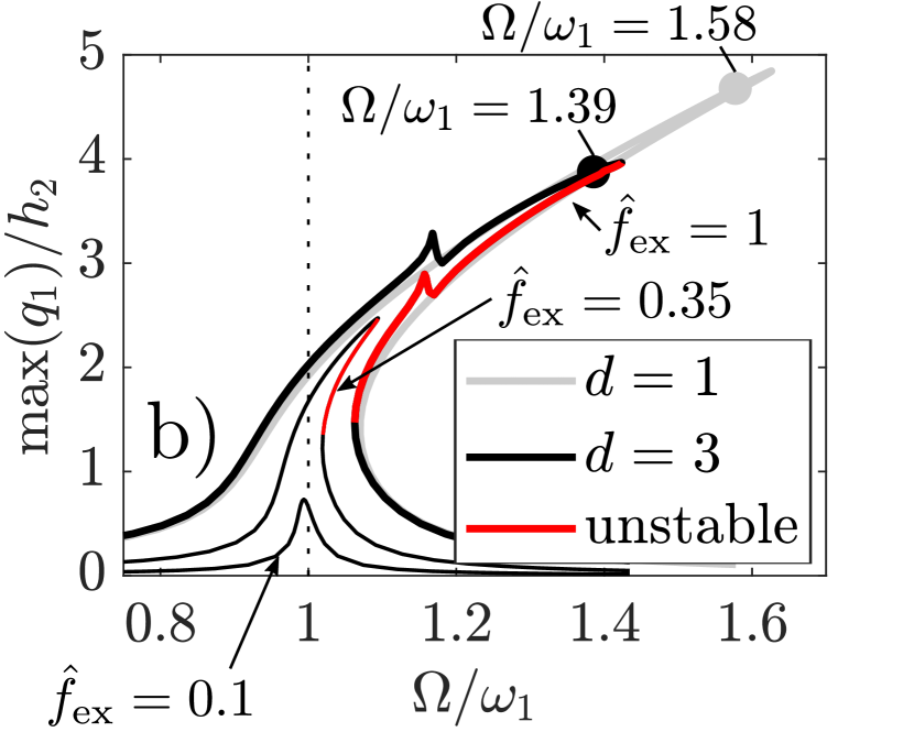
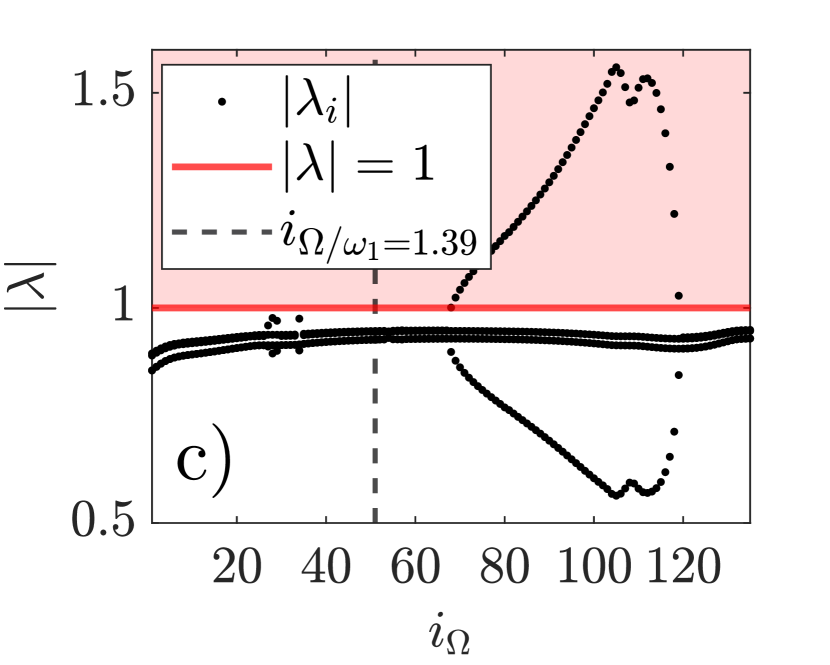
Figure 3: ECL benchmark: (a) schematic illustration of the two connected cantilevered beams, (b) amplitude-frequency curves for different excitation levels, (c) magnitude of Floquet multipliers for the highest excitation level; material properties and geometric dimensions are density $\rho=7800$ kg/m³, Young’s modulus $E=205\cdot 10^{9}$ N/m², beam cross sections $A_{1}=h_{1}\cdot z=0.014\cdot 0.014$ m² and $A_{2}=h_{2}\cdot z=0.0005\cdot 0.014$ m², beam lengths $L_{1}=0.7$ m and $L_{2}=0.04$ m

The ECL benchmark [30] consists of a primary beam connected to a much more slender and shorter beam, as illustrated in Fig. 3a. The model and the selected parameters largely follow [31]. The dimensions and material properties are specified in the caption of Fig. 3. At the connection between the beams, a cubic spring with stiffness coefficient $k_{3}=8\cdot 10^{9}\,$N/m³ and a quadratic spring with stiffness coefficient $k_{2}=-1.05\cdot 10^{7}\,$N/m² is considered, modeling the hardening due to bending-stretching and the softening due to non-ideal clamping of the thinner beam, respectively. In contrast to [31], no finite rotational stiffness between the two beams is introduced, but instead a rigid rotational connection is modeled. An FE model involving 1000 beam elements was set up, followed by a modal truncation to the lowest-frequency bending modes of the linearized system ($d=1$ or $d=3$). For consistency with [31], Euler-Bernoulli elements are used, although Timoshenko elements should generally be preferred to account for shear within short beam elements. Moreover, Rayleigh damping is considered, where the mass and stiffness coefficients are given by $\alpha=3\cdot 10^{-7}$ and $\beta=5$, respectively, resulting in a modal damping ratio of $D_{1}=1.2\%$ for the fundamental bending mode.
A harmonic concentrated load, $f_{\mathrm{ex}}=\hat{f}_{\mathrm{ex}}\cos(\Omega t)$, is applied at the connection point. The amplitude-frequency curves of the periodic steady-state response are depicted for different excitation levels $\hat{f}_{\mathrm{ex}}$ in Fig. 3b in the frequency range around the fundamental bending mode (natural angular frequency $\omega_{1}$). The fundamental bending mode shape is also illustrated in Fig. 3a. As amplitude measure, the maximum (along the period) bending displacement at the connection point is used. A slight softening and a pronounced hardening effect can be observed, as expected for the given signs and magnitudes of $k_{2}$, $k_{3}$. Also as expected for light damping, the amplitude-frequency curves exhibit turning points for sufficiently large excitation level. In addition, a secondary resonance phenomenon is encountered for $\hat{f}_{\mathrm{ex}}=1$ in the configuration with three retained modes, $d=3$, as opposed to configuration with only one mode, $d=1$. As expected, the overhanging branch connecting the turning points is unstable. This is confirmed by the Floquet multipliers, whose magnitude is depicted in Fig. 3c along the branch obtained for $\hat{f}_{\mathrm{ex}}$. Herein, $i_{\Omega}$ denotes the index of the solution point along the branch. A single Floquet multiplier leaves the unit disk, as expected for turning point bifurcations.

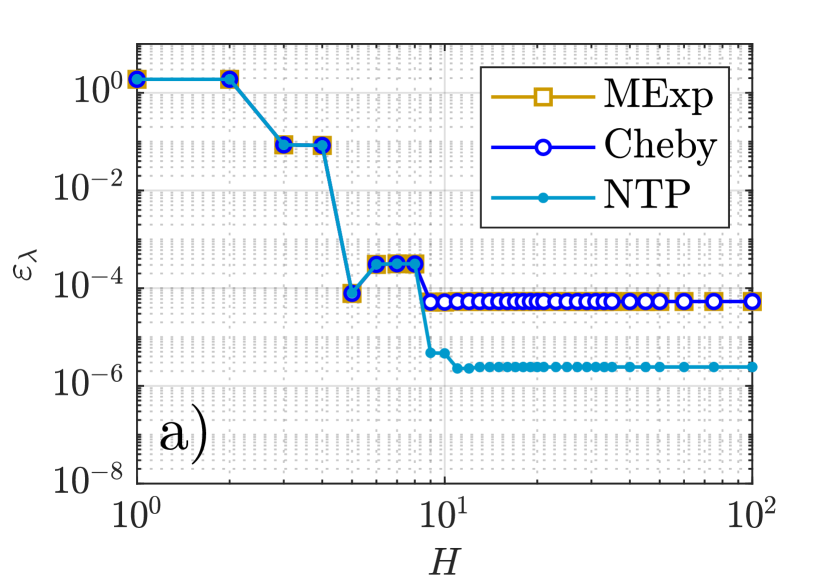
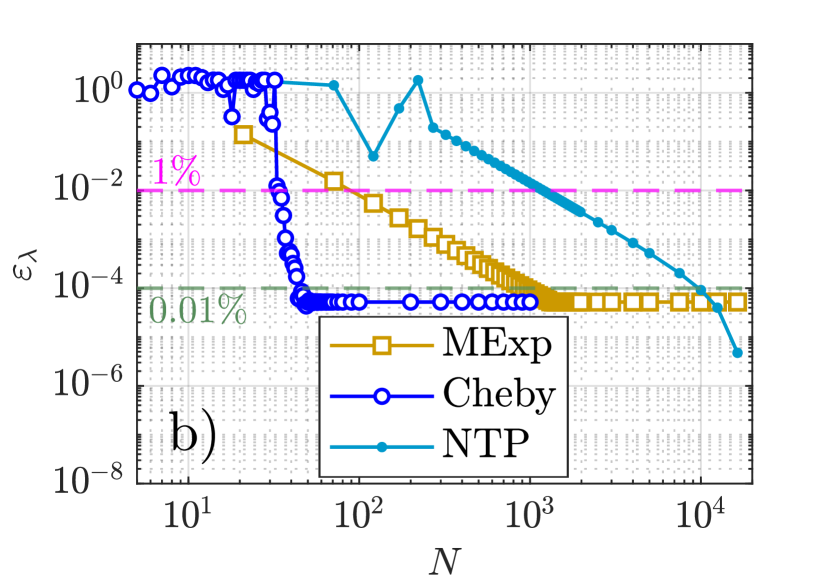
Figure 4: ECL benchmark: Leading Floquet multiplier error (a) vs. $H$, (b) vs. $N$ for the point with $\Omega/\omega_{1}=1.39$ ($d=3$) indicated in Fig. 3b

To assess the performance of the Chebyshev-based method of stability analysis (Cheby), the error with respect to the leading Floquet multiplier $\lambda_{\mathrm{l}}$ is considered,

$$\varepsilon_{\lambda}=\left|\lambda_{\mathrm{l}}-\lambda_{\mathrm{l,ref}}\right|\,,$$ (35)

where the reference $\lambda_{\mathrm{l,ref}}$ is obtained by the Shooting method in conjunction Newmark’s time step integration scheme (constant-average-acceleration variant) with $N=2^{14}$ time levels per period. The monodromy matrix $\boldsymbol{\Phi}(2\pi)$ is obtained as a by-product of Shooting. The results are confronted with the Matrix Exponential (MExp) and the Newmark Method (NTP) of stability analysis, as described in Subsection 2.4. Many different solution points and model parameters (such as excitation levels and modal truncation orders) were analyzed. Results are only shown for a representative point, namely that with $\Omega/\omega_{1}=1.39$ indicated in Fig. 3b. The $H$-convergence is illustrated in Fig. 4a. The number of samples within the Alternating Frequency-Time scheme was set sufficiently large to avoid aliasing errors. The time resolution during the integration of $\boldsymbol{\Phi}$ was set sufficiently large to ensure that this does not have any visible effect on the depicted results. Apparently, $H=5$ is sufficient to have an error $\varepsilon_{\lambda}$ smaller than $1\%$. The individual round-off plateaus are reached at $H=9$. The round-off plateau for the Newmark Method is slightly lower, which is attributed to the fact that essentially the same code is used as in the case of the reference method.
In Fig. 4b, the $N$-convergence is illustrated for $H=9$. Recall that generally $N\neq N_{\mathrm{AFT}}$; in fact, $N_{\mathrm{AFT}}=4H+1$ is sufficient to avoid aliasing for the given nonlinearity. Thus, $N$ does not affect the HB approximation but only determines the time resolution within the stability analysis. For the Chebyshev Method, it holds that $C=N$, as explained in Subsection 2.4. Apparently, the Chebyshev Method achieves high accuracy already with a coarser time resolution than the other methods. In practice, it may be a delicate issue to properly select $C$. It is well-known that for the task of approximating a harmonic function of order $H^{*}$, the required $C$ approaches $\pi H^{*}$ for large $H^{*}$, see [25] (ch. 2.14). Thus, if $H$ is the highest (non-negligible) harmonic, the cubic nonlinearity generates as highest harmonic $3H$, $C$ should be selected larger than $3\pi H$ (e. g. $C=85$ for $H=9$). Apparently, this is a good yet somewhat conservative empirical rule for the considered example.

Table 1: Computation effort of stability analysis for the error threshold $\varepsilon_{\lambda}<1\%$ and $\varepsilon_{\lambda}<0.01\%$ (offline computation effort for Cheby given in brackets): ECL benchmark with $d=1$ for $\Omega/\omega_{1}=1.58$ ($\varepsilon_{\lambda}<1\%$: $C=19$, $N_{\mathrm{NTP}}=N_{\mathrm{MExp}}=121$); ECL benchmark with $d=3$ for $\Omega/\omega_{1}=1.39$ ($\varepsilon_{\lambda}<1\%$: $C=35$, $N_{\mathrm{NTP}}=1221$, $N_{\mathrm{MExp}}=121$; $\varepsilon_{\lambda}<0.01\%$: $C=45$, $N_{\mathrm{NTP}}=10001$, $N_{\mathrm{MExp}}=971$); two-degree-of-freedom oscillator with elastic stop ($\varepsilon_{\lambda}<1\%$: $C=600$, $N_{\mathrm{MExp}}=1001$, $N_{\mathrm{NTP}}=1501$); the given computation times represent mean values based on $10,000$ repeats; solution points are indicated in Fig. 3b, Fig. 6a, respectively.

	ECL benchmark ($d=1$)	ECL benchmark ($d=3$)		2DOF oscillator with elastic stop
	$\varepsilon_{\lambda}<1\%$	$\varepsilon_{\lambda}<1\%$	$\varepsilon_{\lambda}<0.01\%$	$\varepsilon_{\lambda}<1\%$
MExp	0.00364s	0.00364s	0.02293s	0.04289s
NTP	0.00087s	0.00281s	0.02593s	0.02700s
Cheby	0.00022s	0.00050s	0.00052s	0.12415s
(offline)	(0.00014s)	(0.00034s)	(0.00036s)	(0.07682s)

Now, we analyze the computational effort. It is useful to recall that all methods of stability analysis need to re-evaluate the Jacobian $\boldsymbol{J}$ with $N<<N_{\mathrm{AFT}}$. Subsequently, their algorithms differ. The Matrix Exponential Method computes a product of $N$ matrix exponentials of dimension $2d$. The Newmark Method solves a sequence of $N$ linear equations of dimension $d$ (with $2d$-dimensional right hand side). The Chebyshev Method solves a single linear equation of dimension $dC$ (with $2d$-dimensional right hand side), where $C$ is linked to the time resolution ($C=N$). In Tab. 1, the computation effort needed to meet an error threshold $\varepsilon_{\lambda}<1\%$ is given for $d=1$ and $d=3$, respectively, at the respective solution point indicated in Fig. 3b. For $d=3$, the case of a finer error threshold $\varepsilon_{\lambda}<0.01\%$ is additionally analyzed. All computations were carried out on a Windows 10 machine with a quad-core 4GHz Intel(R) Core(TM) i7-6700K CPU, 32GB RAM using MATLAB R2022a. Since the Chebyshev method converges to the reference solution for much coarser time resolution, $C<N_{\mathrm{NTP}},N_{\mathrm{MExp}}$ holds for both error thresholds. With this, the Chebyshev Method speeds up the stability analysis by about one order of magnitude (factor $4$ and $6$ for $d=1$ and $d=3$, respectively) for $\varepsilon_{\lambda}<1\%$ and by about two orders of magnitude (factor $50$ for $d=3$) for $\varepsilon_{\lambda}<0.01\%$. Here, we considered only the online effort. For completeness, the Chebyshev Method’s offline effort is additionally given in brackets in Tab. 1. This includes setting up the matrix of the discrete Chebyshev transform, $\boldsymbol{T}$ and its inverse, the integration operation matrix $\boldsymbol{G}$ (and its products with the linear system matrices), auxiliary matrices for efficient online computation of the product operation matrix $\boldsymbol{P}(\cdot)$, along with the vectors of initial values. This effort scales with the order $C$ and the size of the system matrices $d$, but can be efficiently computed once and for all (for given $d$ and maximum $C$). Thus, this effort becomes quickly negligible during a path continuation task (with many solution points). In comparison, the computation time required to solve for the periodic solution remained of the same order of magnitude as the stability estimation (one Newton iteration step with respect to the HB equations ($H=9$) took $0.9\cdot 10^{-4}$s for $d=1$ and $2.1\cdot 10^{-3}$s for $d=3$ ; usually 3 to 10 iterations are needed per solution point during continuation).

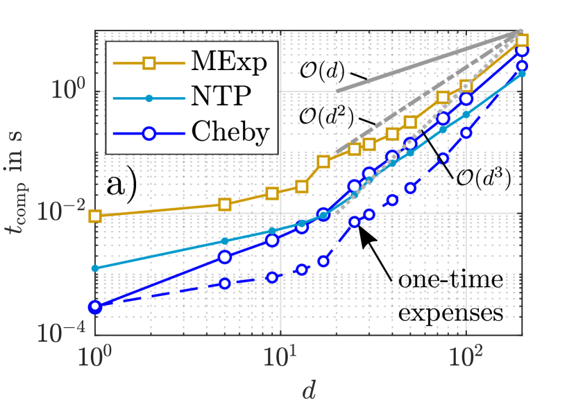
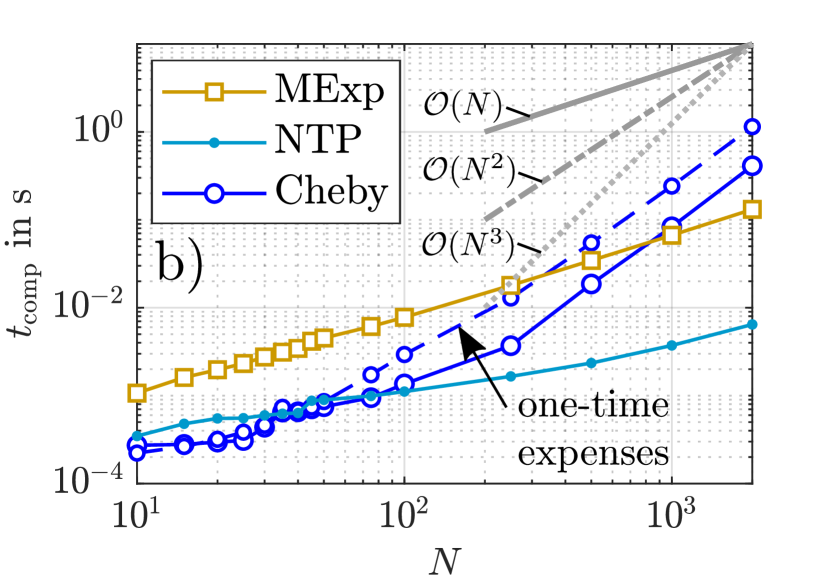
Figure 5: Computation effort of stability analysis for ECL benchmark: (a) scaling with $d$ ($C=19$, $N_{\mathrm{MExp}}=N_{\mathrm{NTP}}=121$), (b) scaling with $N$ ($d=1$). The depicted computation times represent mean values where the number of repeats depend on $d$ and $N$, respectively: 10,000 for the smallest values and still $d=500$ for the largest values.

Next, it is analyzed how the computation effort scales with the number of degrees of freedom $d$ and the time resolution $N$ (Fig. 5). Up to about $d=17$, the Chebyshev Method shows superior computational efficiency. Subsequently, the Newmark Method becomes more efficient, which apparently scales best among the three methods, while the Matrix Exponential Method is slowest. Moreover, the Chebyshev Method scales worst with the time resolution. For the given example, the Newmark Method thus becomes more efficient beyond $N=35$. The relatively poor scaling behavior of the Chebyshev Method seems plausible in the light of the above described main computation task (solving a $dN$-dimensional equation system rather than $N$ sequential $d$-dimensional ones as in the Newmark Method). It can thus be said that the Chebyshev Method can only be attractive, if it overcompensates its poor scaling behavior by superior convergence.

4.2 Two-degree-of-freedom oscillator with elastic stop

We now consider a chain of two spring-mass oscillators described by the equations of motion,

$$\ddot{q}_{1}+0.03\dot{q}_{1}-0.03\dot{q}_{2}+q_{1}-q_{2}+f_{\mathrm{nl}}(q_{1}) =0\,,$$ (36)

$$\ddot{q}_{2}-0.03\dot{q}_{1}+0.06\dot{q}_{2}-q_{1}+2q_{2}-0.1\cos(\Omega t) =0\,.$$ (37)

The unit mass described with coordinate $q_{2}$ is connected via unit springs to the ground and to the unit mass described with coordinate $q_{1}$. Dashpots with damping coefficient $0.03$ are in parallel to these springs. A harmonic forcing is applied to the second mass, while the first mass is subjected to an elastic stop (unilateral spring) with unit clearance and stiffness 100. The nonlinear force, $f_{\mathrm{nl}}(q_{1})$, would thus be given by $100\cdot\mathrm{max}(q_{1}-1,0)$. However, to ensure applicability of Urabe’s and Floquet’s theorems, we consider the smooth (infinitely differentiable) regularization

$$f_{\mathrm{nl}}(q_{1})=\frac{100(q_{1}-1)}{2}+\sqrt{\left(\frac{100(q_{1}-1)}{2}\right)^{2}+\varepsilon_{\mathrm{reg}}}\,.$$ (38)

The steeper the regularization, i. e. the smaller $\varepsilon_{\mathrm{reg}}$, the more will Eq. (38) resemble an elastic stop. The effect of this regularization on the periodic response near the fundamental natural frequency is illustrated in Fig. 6a. In the following, we use $\varepsilon_{\mathrm{reg}}=0.2$. Besides turning points, a Torus bifurcation occurs near $\Omega/\omega_{1}=1$ (close to the transition from quasi-linear to nonlinear regime), and a period doubling bifurcation occurs near the resonance peak. The magnitudes of the Floquet multipliers are depicted in Fig. 6b.

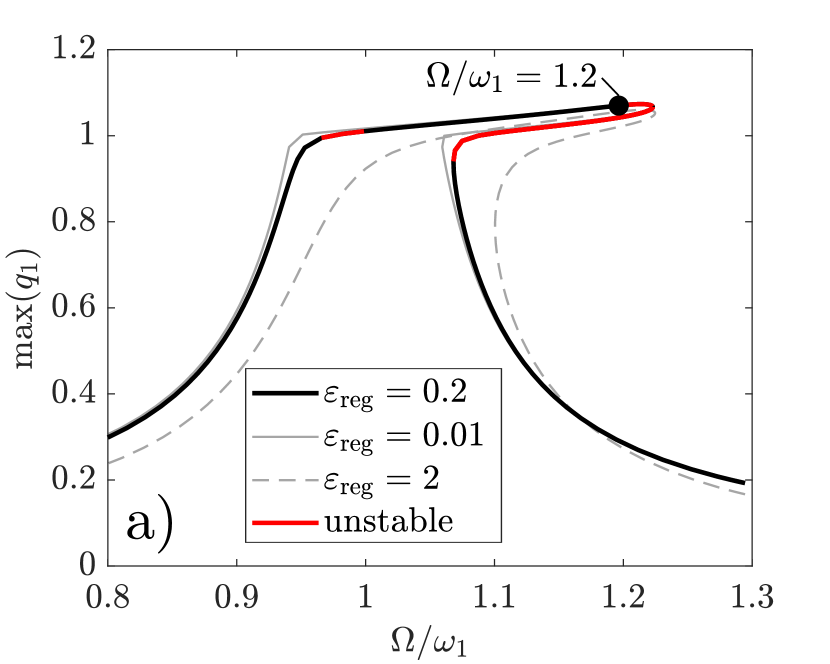
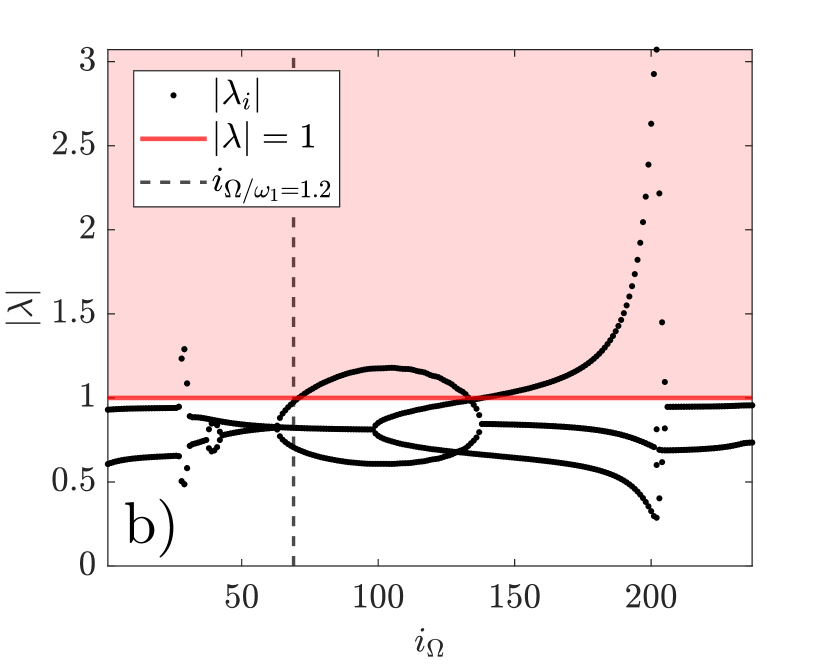
Figure 6: Two-degree-of-freedom oscillator with elastic stop: (a) amplitude-frequency curves for different steepness of regularization $\varepsilon_{\mathrm{reg}}$, (b) magnitude of Floquet multipliers for $\varepsilon_{\mathrm{reg}}=0.2$

As in the previous example, many parameter sets and solution points were studied, but only representative results are shown for brevity, namely for a solution point on the upper branch near the period doubling bifurcation (indicated in Fig. 6, $\Omega/\omega_{1}=1.2$). The results of the $H$- and $N$-convergence are shown in Fig. 7a and b, respectively. The reference for the definition of the leading Floquet multiplier error was again obtained using Shooting, however, a refinement to $N=2^{15}$ time levels was found to be necessary. A much larger truncation order, $H>200$, is needed to reach the round-off plateau, as compared with the case of the cubic nonlinearity. Similarly, a much finer time resolution is needed: To achieve the specified error threshold $\varepsilon_{\lambda}<1\%$ ($H=80$), the minimum number of samples is $C=600$, $N_{\mathrm{MExp}}=1001$, $N_{\mathrm{NTP}}=1501$. Thus, the advantage of the Chebyshev interpolation is much less pronounced for the given type of nonlinearity. In conjunction with the poor scaling, the Chebyshev Method actually becomes inferior (see Tab. 1). More specifically, the Chebyshev Method is by a factor of about $5$ slower than the Newmark Method.

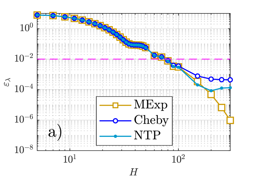
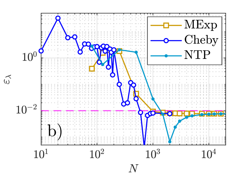
Figure 7: Two-degree-of-freedom oscillator with elastic stop: Leading Floquet multiplier error (a) vs. $H$, (b) vs. $N$ for the point with $\Omega/\omega_{1}=1.2$ indicated in Fig. 6

5 Numerical results: Error bound

Two numerical examples are considered in this section: First, the forced-damped Duffing oscillator with softening characteristic is analyzed, where we shall rigorously prove the existence of some isolated solutions. Second, the two-degree-of-freedom oscillator with elastic stop from Subsection 4.2 is revisited.

5.1 Duffing oscillator with softening characteristic

The Duffing oscillator is the archetype of a nonlinear dynamical system. In the case of a negative coefficient of the cubic spring (softening characteristic), an isolated branch of frequency responses, emerging from zero excitation frequency, is commonly depicted in textbooks. In [13], it has been questioned whether such isolated solutions actually exist. We consider the specific equation of motion,

$$\ddot{q}+0.12\dot{q}+q-0.1q^{3}=0.2\cos(\Omega t)\,.$$ (39)

Fig. 8 shows the amplitude-frequency curve. As expected for the softening characteristic, the main branch is bent towards the left giving rise to two turning points. Moreover, an isolated branch occurs. In fact, multiple of such isolated branches appear as solutions of the HB equations [13]; in this work, we study only a representative one. While there is a scientific debate concerning the existence of an exact periodic solution, there is consensus that if the solution exists, it will be unstable. Hence, the existence of these solutions is of rather academic interest.

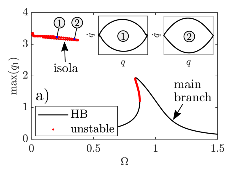
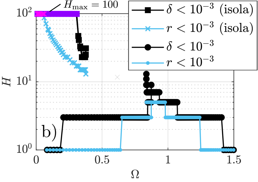
Figure 8: Duffing oscillator with softening characteristic: (a) amplitude-frequency curve, (b) harmonic order obtained by adaptive refinement during path. If the adaptive $H$-refinement reaches the maximum value ($H=100$), the existence of an exact solution could not be proven within the error threshold (indicated by ’pink’ and ’purple’ markers).

The method described in Section 3 is now applied in order to analyze the existence of an exact periodic solution and to obtain an error bound. To this end, an upper bound, $\Delta(\delta)$, for the variation of the Jacobian in the $\delta$-neighborhood of the $H$-order approximation, $q_{H}$, is needed, so that

$$\Delta(\delta){\leq}\max_{\tau}\left|-0.1\cdot 3\cdot\left(\left(q_{H}\left(\tau\right)+\delta\right)^{2}-q_{H}^{2}\left(\tau\right)\right)\right|\,.$$ (40)

One can see that the expression on the right increases monotonically with $q_{H}$. Thus, an upper bound for $q_{H}(\tau)$ (truncated Fourier series) must be found, which is straight-forward to obtain. The number of samples within the Alternating Frequency-Time scheme is set to $N_{\mathrm{AFT}}=4H+1$ to ensure that aliasing is avoided. The time resolution for Chebyshev interpolation is set to $C=5H$, which was found sufficient to ensure that the depicted results do not visibly change for a further increase of $C$.
The computation of the error bound is used in an adaptive $H$-refinement, embedded into a numerical path continuation scheme. The algorithm reads as follows:

1. Start the continuation with $H=1$.

2. Compute $r$, $M$ as proposed in Section 3.

3. If a finite error bound $\delta$ can be given, and $H$ was increased at least once such that $\delta(H-2)>10^{-3}$ and $\delta(H)\leq 10^{-3}$, go to 5. Otherwise go to 4.

4. If $\delta>10^{-3}$: If $H=H_{\max}$, go to 5. Otherwise increase $H\rightarrow H+2$ and go to 2.
   Otherwise ($\delta\leq 10^{-3}$): If $H=H_{\min}$, go to 5. Otherwise decrease $H\rightarrow H-2$ and go to 2.

5. Do the next step of the continuation.

The limits of $H_{\max}=100$ and $H_{\min}=1$ are specified. Using this algorithm, we obtain the minimum harmonic truncation order, $H$, required to satisfy a certain convergence criterion with respect to $\delta$. The results are shown in Fig. 8b, both for the main and the isolated branch. Additionally, results are shown for the case where the convergence criterion in step 3-4 of the above algorithm is replaced by the simple condition $r<10^{-3}$. It should be emphasized that $r$ and $\delta$ have quite different physical meanings: While $r$ is the (time-domain) residual of a dynamic force balance, $\delta$ is an error bound between approximation and exact solution in the state space. Thus, using the same numerical threshold $10^{-3}$ is arbitrary and has no justification. Regarding the number of required $H$, see Fig. 8b, the condition $r<10^{-3}$ is weaker than $\delta<10^{-3}$; i. e., $r<10^{-3}$ does not imply $\delta<10^{-3}$, but it can be confirmed that HB approximations that satisfy $\delta<10^{-3}$ all have $r<10^{-3}$. It should further be noted, that the actual error bound $\delta$ (or time domain residual $r$) may be well below the specified threshold value. For some points near the tip of the isolated branch, the existence of a periodic solution in the corresponding $\delta$-neighborhood can be rigorously proven , associated with an harmonic truncation order $H_{\mathrm{min}}\leq H<H_{\mathrm{max}}$. As $\Omega\to 0$, both $H$-refinement algorithms run into the limit $H=H_{\max}$, leading to inconclusive existence results in a certain range (indicated by ’pink’ and ’purple’ markers).

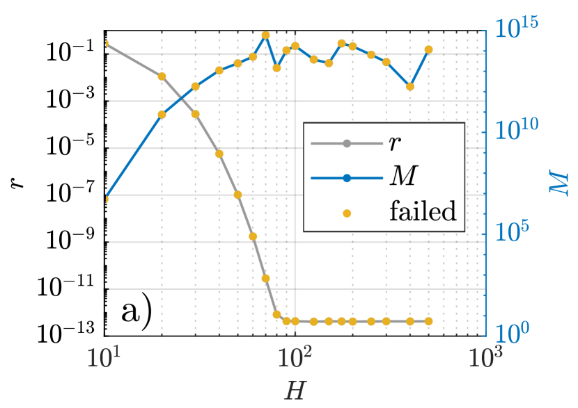
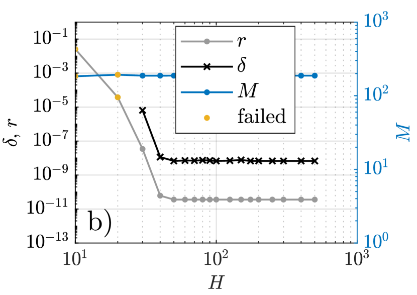
Figure 9: Duffing oscillator with softening characteristic: $H$-convergence for two points on the isolated branch (a) $\Omega=0.2$, (b) $\Omega=0.35$. For the points indicated as failed (’orange’ markers), no error bound could be determined for the given harmonic order.

Fig. 9 shows the $H$-convergence for the two different points on the isolated branch indicated in Fig. 8a, for which also the phase projections are shown. For $\Omega=0.35$, an error bound can be given from $H\geq 30$; the error bound is $\delta<10^{-5}$. The round-off plateau of $r$ is reached at about $H=50$. Interestingly, the parameter $M$, which is a measure for the error propagation along the cycle, does not change significantly with $H$. Thus, Urabe’s error bound is here mainly driven by the time-domain residual $r$. For $\Omega=0.2$, $M$ is extremely large ($\mathcal{O}(M)\approx 10^{14}$ vs. $\mathcal{O}(M)\approx 10^{2}$ for $\Omega=0.35$), so that no error bound can be given, even when the round-off plateau of $r$ is reached. The high $M$ is attributed to the strongly repelling nature of the corresponding region in the state space. Probably, a higher number precision is needed to obtain an error bound and rigorously prove the existence of an exact solution in the associated $\delta$-neighborhood. The phase projections in Fig. 8a suggest that the cycle is close to a hetero-clinic orbit, for which HB is known to show poor convergence.

5.2 Two-degree-of-freedom oscillator with elastic stop

We now revisit the example of Subsection 4.2. Analogously to the previous example, we have as upper bound for the variation of the Jacobian,

$$\Delta(\delta){\leq}\max_{\tau}\left|~{}\left.\frac{\mathrm{d}f_{\mathrm{nl}}}{\mathrm{d}q_{1}}\right|_{q_{1,H}(\tau)+\delta}~{}-~{}\left.\frac{\mathrm{d}f_{\mathrm{nl}}}{\mathrm{d}q_{1}}\right|_{q_{1,H}(\tau)}~{}\right|\,,$$ (41)

$$\text{where}\quad\frac{\mathrm{d}f_{\mathrm{nl}}}{\mathrm{d}q_{1}}=\frac{100}{2}\left(1+\frac{100(q_{1}-1)}{\sqrt{100^{2}(q_{1}-1)^{2}+4\varepsilon_{\mathrm{reg}}}}\right)\,.$$ (42)

Continuation in conjunction with adaptive $H$-refinement is carried out as in the previous example, only the limit was raised to $H_{\max}=500$. A number of $N_{\mathrm{AFT}}=2^{13}$ samples per period were used within the Alternating Frequency-Time scheme, and an adaptive time resolution with $C=8H$ was used for Chebyshev interpolation. Fig. 10a shows results obtained during continuation of the branch depicted in Fig. 6a. As in the previous example, higher orders $H$ are needed to obtain an error bound $\delta<10^{-3}$ than to reduce the residual below $r<10^{-3}$. In fact, $H=500$ is insufficient near the resonance peak (indicated by ’pink’ markers). For the point with $\Omega/\omega_{1}=1.2$ indicated in Fig. 6a, $H>1000$ is needed to obtain an error bound (Fig. 10b).

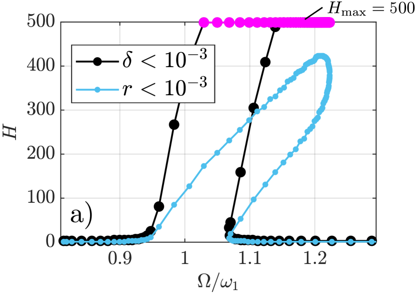
Figure 10: Two-degree-of-freedom oscillator with elastic stop: (a) harmonic order obtained by adaptive $H$-refinement during path continuation. If it reaches the maximum value ($H=500$), the existence of an exact solution could not be proven within the error threshold (indicated by ’pink’ markers). (b) $H$-convergence for the point with $\Omega/\omega_{1}=1.2$ indicated in Fig. 6a. For the points indicated as failed (’orange’ markers), no error bound could be determined for the given harmonic order.

6 Conclusions

The purpose of the present work was to determine whether (a) Chebyshev-based stability analysis and (b) Urabe’s error bound are useful features for Harmonic Balance. The idea of the Chebyshev-based stability analysis is to exploit the properties of Chebyshev polynomials to avoid the time step integration of the monodromy matrix. Indeed, the time integration is replaced by the solution of a single linear algebraic equation system of dimension $dN$ where $d$ is the number of degrees of freedom and $N$ is the number of time levels per period (equal to the number of Chebyshev polynomials). Thus, the method scales quadratically with $N$, in contrast to conventional time step integration (e. g. Newmark or Matrix Exponential Method), which scales linearly with $N$. Consequently, the Chebyshev Method tends to be quicker when only a relatively small $N$ is needed. This is usually the case when also a low harmonic truncation order $H$ is sufficient, as is typically the case for (inherently) smooth nonlinearities. In contrast, in the presence of (sharply regularized) discontinuities, high $H$ and $N$ are typically needed, and the method becomes inefficient. Reasoning that for high $H$, HB itself becomes inefficient compared to alternative methods for computing periodic oscillations, the Chebyshev-based stability analysis is regarded as natural supplement. About one to two orders of magnitude speedup compared to the state-of-the-art alternatives has been found in the corresponding numerical examples. It should be stressed that further potential for computational speedup exists. For the case of local nonlinearities, in particular, the computational burden of solving the large-dimensional equation system could be reduced by a block condensation with pre-computed factorization of the linear (time-invariant) part.
Concerning Urabe’s error bound, a similar distinction should be made with regard to the considered problem class. For inherently smooth problems, Urabe’s theorem appears useful in computational engineering practice. In contrast, in the presence of (sharply regularized) discontinuities, an extremely high truncation order $H$ is needed to reduce the residual sufficiently to obtain a finite error bound. In that case, conventional time step integration of the periodic solution may become faster so that the use of HB becomes somewhat obsolete. As soon as an error bound could be given, for the considered numerical examples, this error bound was so tight that a further increase of the truncation order never seemed reasonable. From a practical perspective, it would be desirable to have a rigorous existence proof and a finite error bound already for much lower truncation orders. Further, the computational effort for obtaining the measures needed for Urabe’s theorem is relatively high, even when Chebyshev polynomials are again used to achieve numerical efficiency. More specifically, the bottleneck is the computation of the measure $M$, which gives an upper bound for the error propagation within the period. Given the popularity of HB in engineering, research towards the mathematically rigorous development of computationally cheaper error bounds is desirable.

Appendix A Chebyshev analysis

According to the integration rule of Chebyshev polynomials,

$$b_{C} =\int a_{C}\mathrm{d}\tau\,,$$ (43)

$$\check{\boldsymbol{b}} =\boldsymbol{G}\check{\boldsymbol{a}}\,,$$ (44)

i. e.; the integral of a Chebyshev polynomial is a Chebyshev polynomial of the same order. The coefficients are obtained as expressed in Eq. (44), using an integration operational matrix $\boldsymbol{G}$, which reads

$$\boldsymbol{G}=\pi\begin{bmatrix}1&1&0&0&\ldots&0\\ -1/4&0&1/4&0&&0\\ -1/3&-1/2&0&1/6&&0\\ 1/8&0&-1/4&0&&0\\ \vdots&&&&\ddots&\dfrac{1}{2(C-1)}\\ \dfrac{-(-1)^{C-1}}{C(C-2)}&&&&\dfrac{-1}{2(C-2)}&0\end{bmatrix},$$ (45)

for the considered case of Chebyshev base functions of the first kind. The factor $\pi$ stems from the considered interval length $[0,2\pi]$ rather than the unit interval $[-1,1]$.
According to the product rule of Chebyshev polynomials, the product, $c=a_{C}b_{C}$ of two Chebyshev polynomials $a_{C}$ and $b_{C}$ is a Chebyshev polynomial of higher order. When only the coefficients up to order $C$ are of interest, these can be expressed as

$$\check{\boldsymbol{c}}=\boldsymbol{P}\left(\check{\boldsymbol{a}}\right)\check{\boldsymbol{b}}\,,$$ (46)

using the product operational matrix

$$\boldsymbol{P}\left(\check{\boldsymbol{a}}\right)=\begin{bmatrix}\check{a}(1)&\check{a}(2)/2&\check{a}(3)/2&\ldots&\check{a}(C)/2\\ \check{a}(2)&\check{a}(1)+\check{a}(3)/2&(\check{a}(2)+\check{a}(4))/2&&\check{a}(C-1)/2\\ \check{a}(3)&(\check{a}(2)+\check{a}(4))/2&\check{a}(1)+\check{a}(5)/2&&\check{a}(C-2)/2\\ \vdots&&&\ddots&\\ \check{a}(C)&\check{a}(C-1)/2&&&\check{a}(1)\end{bmatrix}\,.$$ (47)

References

References

- [1] M. Urabe, Galerkin’s procedure for nonlinear periodic systems, Archive for Rational Mechanics and Analysis 20 (2) (1965) 120–152.
- [2] T. M. Cameron, J. H. Griffin, An alternating frequency/time domain method for calculating the steady-state response of nonlinear dynamic systems, Journal of Applied Mechanics 56 (1) (1989) 149–154. doi:10.1115/1.3176036.
- [3] C. Padmanabhan, R. Singh, Analysis of periodically excited non-linear systems by a parametric continuation technique, Journal of Sound and Vibration 184 (1) (1995) 35–58. doi:10.1006/jsvi.1995.0303.
- [4] M. Krack, J. Gross, Harmonic Balance for Nonlinear Vibration Problems, Springer, 2019. doi:10.1007/978-3-030-14023-6.
- [5] K. C. Hall, J. P. Thomas, W. S. Clark, Computation of unsteady nonlinear flows in cascades using a harmonic balance technique, AIAA Journal 40 (5) (2002) 879–886.
- [6] R. J. Gilmore, M. B. Steer, Nonlinear circuit analysis using the method of harmonic balance—a review of the art. part i. introductory concepts, International Journal of Microwave and Millimeter–Wave Computer–Aided Engineering 1 (1) (1991) 22–37.
- [7] C. S. Hsu, Impulsive parametric excitation: theory, Journal of Applied Mechanics 39 (2) (1972) 551–558.
- [8] P. Friedmann, C. E. Hammond, T.-H. Woo, Efficient numerical treatment of periodic systems with application to stability problems, International Journal for Numerical Methods in Engineering 11 (1977) 1117–1136.
- [9] L. Peletan, S. Baguet, M. Torkhani, G. Jacquet-Richardet, A comparison of stability computational methods for periodic solution of nonlinear problems with application to rotordynamics, Nonlinear Dynamics 72 (3) (2013) 671–682.
- [10] G. v. Groll, D. J. Ewins, The harmonic balance method with arc-length continuation in rotor/stator contact problems, Journal of Sound and Vibration 241 (2) (2001) 223–233. doi:10.1006/jsvi.2000.3298.
- [11] A. Lazarus, O. Thomas, A harmonic-based method for computing the stability of periodic solutions of dynamical systems, Comptes Rendus Mécanique 338 (9) (2010) 510–517.
- [12] Gerald Moore, Floquet theory as a computational tool, SIAM Journal on Numerical Analysis 42 (6) (2005) 2522–2568. doi:10.1137/S0036142903434175.
- [13] U. von Wagner, L. Lentz, On the detection of artifacts in harmonic balance solutions of nonlinear oscillators, Applied Mathematical Modelling 65 (2019) 408–414. doi:10.1016/j.apm.2018.08.013.
- [14] U. von Wagner, L. Lentz, On artifact solutions of semi-analytic methods in nonlinear dynamics, Archive of Applied Mechanics 88 (10) (2018) 1713–1724. doi:10.1007/s00419-018-1397-3.
- [15] A. Grolet, F. Thouverez, On a new harmonic selection technique for harmonic balance method, Mechanical Systems and Signal Processing 30 (2012) 43–60. doi:10.1016/j.ymssp.2012.01.024.
- [16] V. Jaumouillé, J. J. Sinou, B. Petitjean, An adaptive harmonic balance method for predicting the nonlinear dynamic responses of mechanical systems - application to bolted structures, Journal of Sound and Vibration 329 (19) (2010) 4048–4067.
- [17] A. Ferri, M. Leamy, Error estimates for harmonic-balance solutions of nonlinear dynamical systems, in: 50th AIAA/ASME/ASCE/AHS/ASC Structures, Structural Dynamics, and Materials Conference, Structures, Structural Dynamics, and Materials and Co-located Conferences, American Institute of Aeronautics and Astronautics, 2009. doi:10.2514/6.2009-2667.
- [18] A. Stokes, On the approximation of nonlinear oscillations, Journal of Differential Equations 12 (3) (1972) 535–558. doi:10.1016/0022-0396(72)90024-1.
- [19] M. Urabe, A. Reiter, Numerical computation of nonlinear forced oscillations by galerkin’s procedure, Journal of Mathematical Analysis and Applications 14 (1) (1966) 107–140.
- [20] R. van Dooren, On the transition from regular to chaotic behaviour in the duffing oscillator, Journal of Sound and Vibration 123 (2) (1988) 327–339. doi:10.1016/S0022-460X(88)80115-9.
- [21] A. Baker, M. Dellnitz, O. Junge, Topological method for rigorously computing periodic orbits using fourier modes, Discrete and Continuous Dynamical Systems - DISCRETE CONTIN DYN SYST 13 (2005). doi:10.3934/dcds.2005.13.901.
- [22] J.-P. Lessard, C. Reinhardt, Rigorous numerics for nonlinear differential equations using chebyshev series, SIAM J. Numer. Anal. 52 (2014) 1–22. doi:10.1137/13090883X.
- [23] J.-P. Lessard, J. Mireles James, A. Hungria, Rigorous numerics for analytic solutions of differential equations: The radii polynomial approach, Mathematics of Computation 85 (2015). doi:10.1090/mcom/3046.
- [24] F. Kogelbauer, T. Breunung, When does the method of harmonic balance give a correct prediction for mechanical systems?, Applicable Analysis 2 (2021) 1–19. doi:10.1080/00036811.2021.1953482.
- [25] J. P. Boyd, Chebyshev and Fourier spectral methods, Courier Corporation, 2001.
- [26] S. C. Sinha, D. H. Wu, An efficient computational scheme for the analysis of periodic systems, Journal of Sound and Vibration 151 (1) (1991) 91–117. doi:10.1016/0022-460X(91)90654-3.
- [27] D.-H. Wu, S. C. Sinha, A new approach in the analysis of linear systems with periodic coefficients for applications in rotorcraft dynamics, The Aeronautical Journal (1968) 98 (971) (1994) 9–16. doi:10.1017/S0001924000050302.
- [28] L. Woiwode, N. N. Balaji, J. Kappauf, F. Tubita, L. Guillot, C. Vergez, B. Cochelin, A. Grolet, M. Krack, Comparison of two algorithms for harmonic balance and path continuation, Mechanical Systems and Signal Processing 136 (2020) 106503. doi:10.1016/j.ymssp.2019.106503.
- [29] J. D. García-Saldaña, A. Gasull, A theoretical basis for the harmonic balance method, Journal of Differential Equations 254 (1) (2013) 67–80. doi:10.1016/j.jde.2012.09.011.
- [30] F. Thouverez, Presentation of the ecl benchmark, Mechanical Systems and Signal Processing 17 (1) (2003) 195–202. doi:10.1006/mssp.2002.1560.
- [31] J.-P. Noël, L. Renson, C. Grappasonni, G. Kerschen, Identification of nonlinear normal modes of engineering structures under broadband forcing, Mechanical Systems and Signal Processing 74 (2016) 95–110, special Issue in Honor of Professor Simon Braun. doi:https://doi.org/10.1016/j.ymssp.2015.04.016.