Exploring Asymmetric Tunable Blind-Spots for Self-supervised Denoising in Real-World Scenarios

Abstract

Self-supervised denoising has attracted widespread attention due to its ability to train without clean images. However, noise in real-world scenarios is often spatially correlated, which causes many self-supervised algorithms based on the pixel-wise independent noise assumption to perform poorly on real-world images. Recently, asymmetric pixel-shuffle downsampling (AP) has been proposed to disrupt the spatial correlation of noise. However, downsampling introduces aliasing effects, and the post-processing to eliminate these effects can destroy the spatial structure and high-frequency details of the image, in addition to being time-consuming. In this paper, we systematically analyze downsampling-based methods and propose an Asymmetric Tunable Blind-Spot Network (AT-BSN) to address these issues. We design a blind-spot network with a freely tunable blind-spot size, using a large blind-spot during training to suppress local spatially correlated noise while minimizing damage to the global structure, and a small blind-spot during inference to minimize information loss. Moreover, we propose blind-spot self-ensemble and distillation of non-blind-spot network to further improve performance and reduce computational complexity. Experimental results demonstrate that our method achieves state-of-the-art results while comprehensively outperforming other self-supervised methods in terms of image texture maintaining, parameter count, computation cost, and inference time.

1 Introduction

Image denoising is an essential low-level computer vision problem designed to recover clean signals from given noisy observations. With the advancements in deep learning and convolutional neural networks (CNNs), an increasing number of studies are focused on supervised learning using clean-noisy pairs [2, 16, 31, 45, 46, 47]. Typically, additive white Gaussian noise (AWGN) is introduced into clean datasets to synthesize clean-noisy denoising datasets. However, real-world noise is known to be spatially correlated [8, 21, 35], and the simple assumption of synthetic datasets regarding noise can lead to poor generalization in real-world scenarios. Some generative-based methods attempt to synthesize real-world noise from existing clean data [6, 9, 17, 20, 40] and then employ supervised learning. However, synthesizing real-world noise remains challenging, and unpaired methods still suffer from the issue of mismatch between the distribution of existing clean data and the desired scenario. To address the issue, some researchers attempt to capture clean-noisy pairs in real-world scenarios [1, 4]. A typical work is the SIDD dataset [1], which consists of clean-noisy pairs captured under various scenes and illuminations. These datasets enable supervised training on real-world data directly [2, 16, 29, 45, 46]. However, constructing such datasets can be extremely laborious and time-consuming work. In certain scenarios, such as medical imaging and electron microscopy, constructing such datasets can be impractical or even infeasible. These limitations curtail the scope of supervised denoising algorithms.

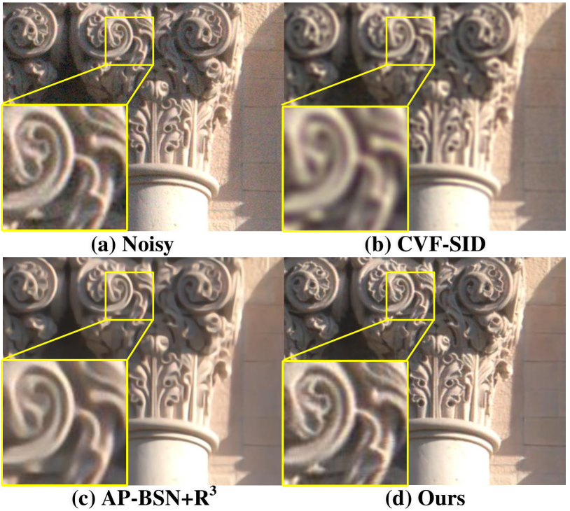
Figure 1: Comparison of our AT-BSN and other methods on the DND benchmark dataset [36]. (a) CVF-SID [33] and (b) AP-BSN [26] are two self-supervised algorithms designed for real-world noise removing, both are trained with only noisy images. Our method preserves the most details while removing noise.

Self-supervised denoising algorithms, represented by Noise2Noise [27], have brought new life to the denoising field. These methods only require noisy observations to train the denoising model. However, in real-world scenarios, noise often exhibits spatial correlation, which contradicts the pixel-wise independent noise assumption [23, 27] that most self-supervised algorithms [3, 19, 23, 27, 39] rely on. As a result, despite their ability to train directly on noisy images, self-supervised denoising algorithms perform poorly in real-world scenarios.

Recent studies have proposed self-supervised denoising algorithms suitable for real-world scenarios [26, 33]. The current state-of-the-art approach AP-BSN [26] utilized pixel-shuffle downsampling (PD) [26, 49] to disrupt the spatial correlation of real-world noisy images and employed asymmetric PD stride factors for training and inference. Furthermore, they proposed random-replacing refinement (R³)[26] post-processing to further improve the performance. However, AP-BSN suffers from various limitations, such as global structure destruction, high-frequency detail loss caused by aliasing effect, and time-consuming inference process.

In this paper, we propose a novel paradigm to break the spatial correlation of noise for real-world self-supervised learning while avoiding the issues of the methods mentioned above. To be specific, we propose a novel BSN with tunable blind-spot size, where a larger blind-spot is used during training to mask only local neighboring pixels to break the local spatial correlation of noise. Compared to AP-BSN, our blind-spot strategy causes minimal damage to the image structure and the global information, allowing the network to learn from all pixels outside the blind-spot for signal restoration, resulting in a larger effective receptive field. During inference, we use a smaller blind-spot to further reduce the loss of local neighboring signals. Since no downsampling process is used, no post-processing is required to mitigate aliasing artifacts.

To implement a BSN with tunable blind-spot sizes, we adapted the original approach proposed by [24]. We further introduce blind-spot self-ensemble to integrate the advantages of different blind-spot sizes. However, the four-fold input of the network results in computational redundancy. To address this issue, we propose to distill the knowledge of blind-spots in different sizes into a lightweight non-blind-spot network (NBSN). Ultimately, we employed the lightweight NBSN for efficient inference.

The main contributions are summarized as follows:

• We present a novel paradigm to break the spatial correlation of real-world noise while causing less damage to the global structure. We propose a tunable blind-spot strategy and employ asymmetric blind-spot sizes for training and inference, respectively.

• To further improve the performance and tackle the computational redundancy in BSN, we propose blind-spot self-ensemble and distill the knowledge of blind-spots in different sizes to a lightweight and computationally efficient Non-BSN for inference.

• Experimental results on real-world datasets demonstrate that our method outperforms the other self-supervised methods with fewer parameters and less inference time. In addition, qualitative results show that our method is capable of recovering more texture information, producing desirable results.

2 Related Work

Supervised Image Denoising. Deep learning has made remarkable advances in image denoising in recent years. Zhang et al. [46] introduced DnCNN, the first CNN-based method for supervised denoising, which significantly outperformed traditional methods [7, 12, 13, 15, 37].The following work aimed to enhance the performance of supervised denoising, such as FFDNet [47], CBDNet [16], RIDNet [2], DANet [45], FADNet [31], and so on. However, supervised-based methods require large amounts of aligned clean-noisy pairs as training data, which are usually difficult and costly to obtain in formal scenarios.

Unpaired Image Denoising. To tackle the challenge in supervised learning, some generative-based [14] approaches synthesize noisy samples from clean images [6, 9, 17, 20, 40]. The simulated clean-noisy pairs can be further used to train a supervised denoising model. However, the performance of unpaired image denoising methods can be limited when the existing clean images do not match the distribution of the current scene.

Self-Supervised Image Denoising. Lehtinen et al. [27] proposed Noise2Noise, which demonstrated that a denoising network could be trained with two independent noisy observations of the same scene. However, even if Noise2Noise relaxes the clean image requirement, obtaining two aligned noisy images in real-world scenarios remains difficult. Noise2Void [23] and Noise2Self [3] proposed a blind-spot strategy to learn denoising from only single noisy images. Further works [24, 40] extended the paradigm to blind-spot network (BSN) through shifted convolutions [24] and dilated convolutions [40]. Blind-spot means the network is designed to denoise each pixel from its surrounding spatial neighborhood without itself, thus, the identity mapping to the noisy image itself can be avoided. Noisier2Noise [32], Noisy-As-Clean (NAC) [41], Recorrupted-to-Recorrupted (R2R) [34], and IDR [48] generated noisy training pairs by adding synthetic noise to given noisy inputs. Recently, Neighbor2Neighbor [19] proposed to subsample the noisy input images to obtain noisy pairs for Noise2Noise-like training. Blind2Unblind [39] proposes a global-aware mask mapper and re-visible loss to fully excavate the information in the blind-spot for Noise2Void-like training.

Real-World Image Denoising. Some works [1, 4] attempt to capture clean-noisy pairs in real-world scenarios. Abdelhamed et al. [1] carefully took and aligned clean-noisy pairs from different scenes and lighting conditions using five representative smartphone cameras, and proposed the SIDD dataset. These datasets enable supervised methods [11, 18, 22, 29, 44, 45] to train on real-world clean-noisy pairs. However, constructing real datasets requires tremendous human effort and time. Moreover, real-world noise tends to exhibit spatial correlation, which contradicts the premise of Noise2Noise [27] that noise follows an independent and identically distributed pattern, rendering it and its subsequent variants unsuitable for direct application to real-world scenarios. In order to apply self-supervised learning to real-world settings, Neshatavar et al. [33] introduced a cyclic multi-variate function to disentangle clean images, signal-dependent noise, and signal-independent noise from noisy images. However, the method relies on a simple network without residual connections to avoid learning an identity mapping to the noise signal. Additionally, the simple assumption about real-world noise signals has resulted in its vague denoising results. Lee et al. [26] employed pixel-shuffle downsampling (PD) [49] to disrupt the spatial correlation of noise and introduced different PD stride factors for training and inference for better performance.

3 Motivation

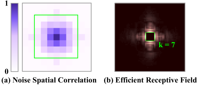
Figure 2: (a) Spatial correlation on real-world noise. The depth of color represents the degree of correlation. We find the correlation becomes negligible outside of the green $7\times 7$ patch. (b) The ERF of our AT-BSN during training. The size of the blind-spot is $7\times 7$.

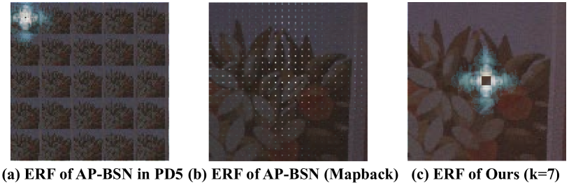
Figure 3: Effective Receptive Field analysis of AP-BSN and our AT-BSN. We adopt the UNet-like BSN proposed by Laine et al. [24] for both methods for a fair comparison. ERFs are superimposed on top of the images and displayed in blue color.

Due to the effect of image signal processors (ISP), e.g. image demosaicking [8, 21, 35], real-world noise is generally known to be spatially correlated and pixel-wise dependent. Lee et al. [26] analyzed the spatial correlation of real-world noise and found that different camera devices in the SIDD dataset show similar noise behaviors in terms of spatial correlation. According to Fig. 2(a), the correlation of noise presents a Gaussian distribution that decays as distance increases. This correlation of noise violates the pixel-wise independent noise assumption of the BSN, rendering it inadequate for real noise removal.

The state-of-the-art algorithm AP-BSN [26] employs asymmetric PD to suppress the spatial correlation. Nevertheless, it suffers from various limitations, such as global structure destruction, high-frequency detail loss caused by the aliasing effect, and a time-consuming inference process.

In this Section, we revisit the framework of AP-BSN, analyze and discuss its limitations. In the next Section, we will modify a classical BSN to address the issues of AP-BSN.

3.1 AP-BSN Revisit

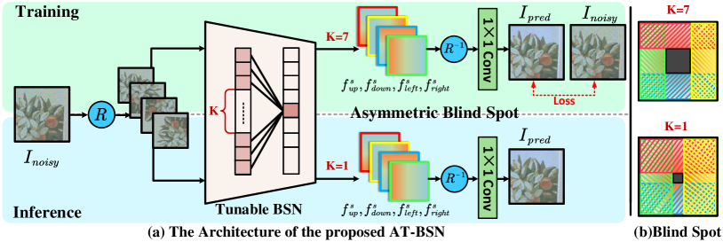
Figure 4: Overview of the proposed AT-BSN framework. (a) We employ asymmetric blind-spots for training and inference to balance the suppression of noise spatial correlation and local information preservation. The rotated input is fed into the network, and then the output features are shifted by $s$ pixels, restricting the receptive field to grow in only one half-plane direction beyond $s$ rows above the current location. Afterward, the features are rotated back and linearly combined through $1\times 1$ convolutions, resulting in a binld-spot with the size of $k=2s-1$. (b) Illustrations of asymmetric blind-spots for training and inference.

AP-BSN employs asymmetric PD stride factors for training and inference in conjunction with BSN. During training, AP-BSN uses PD with stride factor 5 to suppress the spatial correlation between noise signals in training samples. To be specific, a dilated convolutions based BSN $B_{\theta}(\cdot)$ is applied to the downsampled images $PD_{5}{(I_{noisy})}$, where the PD-inverse operation $PD_{5}^{-1}(\cdot)$ follows to reconstruct a full-sized output $I_{pred}$. AP-BSN aims to minimize the following loss function:

$$\mathcal{L}_{apbsn}={\|PD_{5}^{-1}(B_{\theta}(PD_{5}{(I_{noisy})}))-I_{noisy}\|}_{1}$$ (1)

During inference, AP-BSN adopts the PD stride factor of 2 to achieve a balance between aliasing artifacts and noise correlation breaking.

However, AP-BSN suffers from the following issues: 1) The PD process unavoidably destruct detailed textures and global structures, posing challenges for the model to learn the necessary clues for recovering the clean signal. 2) The aliasing artifacts still persist even with the smallest PD stride factor during inference, which leads to the loss of high-frequency information. 3) Moreover, AP-BSN proposed R³ post-process to reduce the aliasing artifacts by averaging 8 noisy images synthesized from the initially denoised results. Nevertheless, R³ operations not only result in a significant increase in inference time but also introduce blurring.

3.2 Effective Receptive Field Analysis of AP-BSN

During training, using PD to disrupt the spatial correlation of noise also disrupts the spatial correlation of the clean signal, which destructs detailed textures and global structures of images. Moreover, noise correlation is generally confined to local regions, according to Lee’s statistics [26] and Fig. 2. Therefore, it is unnecessary to disrupt regions beyond the local neighbors of a pixel. We utilize Effective Receptive Field (ERF) [30] to explicate this point. We consider the ERF of the central pixel. Fig. 3 shows the noisy image and PD result with stride factors of 5, which is used for AP-BSN training. Fig. 3(a) illustrates that the central pixel has been moved to the top left, as well as its ERF. Fig. 3(b) presents the ERF mapped back to the original position.

One can find that the ERF of AP-BSN in the original image manifests as a sparse grid-like pattern, akin to the effect of simple stacking of dilated convolutions [43]. This characteristic comes with similar drawbacks to the dilated convolutions [10, 38, 43], namely 1) the loss of local information, posing challenges for the model to learn clues from the grid-like discontinuous sub-image for recovering the clean signal, and 2) long-ranged information might be not relevant. Moreover, the loss of information continuity can also introduce aliasing artifacts.

From Fig. 3(c), it is apparent that our AT-BSN only loses a portion of the information within the blind-spot area, while the ERF outside the blind-spot remains unaffected. Also see Fig 2, the $7\times 7$ green box covers the main areas in the noise correlation map. This inspires us to set the size of blind-spot to 7 during training. Due to the higher correlation of the signal compared to the noise, the central pixel can be recovered using the pixels outside the blind-spot that are less correlated with it in the noise domain. It is worth noting that the size of the blind-spot can be minimized during inference to reduce information loss.

4 Method

4.1 Tunable Blind-Spot

BSN [23, 26, 40] is designed to denoise each pixel from its surrounding spatial neighborhood without itself. Thus, the identity mapping to the noisy image itself can be avoided. Typically, BSN can be constructed through shifted convolutions [24] or dilated convolution [40]. We will modify the version of Laine’s BSN  [24] .

Restricted Receptive Fields. Our AT-BSN is inspired by Laine’s approach [24], which combines four branches with restricted receptive fields, each of which is limited to a half-plane that excludes the central pixel. Specifically, we modify the convolution and pooling layers of the network, restricting the receptive field to grow in only one half-plane direction, such as upwards.

In convolution layers, we choose zero-padding and shift the feature maps downwards before the convolution operation. For a convolution kernel of size $h\times h$, a downwards offset of $d=\lfloor h/2\rfloor$ pixels is needed. We append $d$ rows of zeros at the top of the feature map, apply the convolution, and finally crop the last $d$ rows of the feature map to achieve the desired shift operation.

In the pooling layer, we perform a $2\times 2$ average pooling operation. Similarly, we add one row of zeros at the top of the feature map and crop the last row of the feature map before pooling to implement the shift operation. As the receptive field of the downsampling layer has already been restricted, we do not need to modify the upsampling layer.

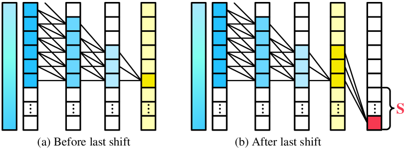
Figure 5: Implementation principle of the tunable blind-spot. The leftmost column of each figure is the input, and the network becomes deeper from left to right. The feature map obtained after each convolution is shown in the middle of each figure. (a) Before the last shift operation $M(\cdot;s)$, the receptive field includes the central pixel itself. (b) After the last shift $M(\cdot;s)$, a blind-spot area is obtained by shifting $s$ pixels. The rightmost layer is the feature map obtained after $1\times 1$ convolutions.

Tunable Blind-Spot. After applying a series of modified convolution and pooling layers together with upsampling layers to the input noisy image $I_{noisy}$, we obtain the resulting feature map denoted as $f_{up}$, whose receptive field is fully contained within an upward half-plane, including the center row. Note that the receptive field at this point includes the pixel itself. See Fig. 5 for more details.

To exclude the center pixel from the receptive field, we shift the feature map $f_{up}$ downward by $s$ pixels, resulting in a shifted feature map $f_{up}^{s}$.

$$f_{up}^{s}=M(f_{up};s),$$ (2)

where $M(\cdot;s)$ denotes the shift operation of a factor $s$. At this point, the receptive field of the central pixel only includes the positions beyond $s$ rows above the current location. And then, to expand the receptive field of a pixel to all directions around it, we rotate the input image by multiples of $90^{\circ}$ and feed them into the network. This results in feature maps $f_{up}^{s}$, $f_{down}^{s}$, $f_{left}^{s}$, and $f_{right}^{s}$, each with its receptive field limited to its respective half-plane. Finally, the four feature maps are rotated to the correct orientation and linearly combined through several $1\times 1$ convolutions $h(\cdot)$ to produce the final output $I_{pred}$.

$$I_{pred}=h([\hat{f}_{up}^{s},\hat{f}_{down}^{s},\hat{f}_{left}^{s},\hat{f}_{right}^{s}]),$$ (3)

where $[,]$ denotes feature concatenation, $\hat{f}^{s}$ denotes the corresponding $f^{s}$ in the correct orientation.

Now for a given pixel, its receptive field is composed of the receptive fields from four different orientations, while a blind-spot area with a length of $k=2s-1$ is formed in the center around it. We can freely tune the size $k$ of the blind-spot by adjusting the shift factor $s$ of the feature map $f^{s}$ before the $1\times 1$ convolutions. So far, we have achieved a BSN with a tunable blind-spot size. We denote the whole network parameterized by $\theta$ as $F_{\theta}(\cdot;s)$, the entire process can be formulated as:

$$I_{pred}=F_{\theta}(I_{noisy};s).$$ (4)

4.2 Asymmetric Blind-Spots

In real-world scenarios, the pixel-wise independent noise assumption of BSN is not satisfied. For smaller blind-spots, the central pixel can be inferred using the neighboring noisy pixels as clues. Based on the fact that the noise correlation is less than the signal correlation, we can use larger blind-spots to suppress the noise correlation while minimizing the impact on signal correlation. The central pixel within a large blind-spot can be inferred from pixels outside the blind-spot that are less correlated with it in the noise domain. During training, we aim to minimize the spatial correlation of noise by setting appropriate blind-spot size $k$ to achieve self-supervised learning of BSN. We minimize the following loss to train the network:

$$\mathcal{L}_{atbsn} ={\|F_{\theta}(I_{noisy};s)-I_{noisy}\|}_{1}$$

$$={\|I_{pred}-I_{noisy}\|}_{1}$$ (5)

Following AP-BSN, we use $L^{1}$ norm for better generalization [26]. In practice, we choose $k=7$, that is, $s=4$, during training.

During inference, the selection of the blind-spot size requires a trade-off between information loss and the level of disruption to the noise spatial correlation. We propose to achieve a balance between training and inference by employing asymmetric blind-spots. Since larger blind-spots have already been utilized during training to enable the BSN to learn to denoise, we can select smaller blind-spots during inference to minimize information loss. Our experiments demonstrate that $k=1$ or $k=3$ during testing leads to better results. Additionally, since our method does not involve downsampling, it avoids aliasing effects and better preserves image texture. The overall scheme can be found in Fig. 4. In Sec. 5.4, we will demonstrate the robustness of our approach to different blind-spot settings.

TABLE I: Comparison among different denoising methods on real-world datasets. Note that at the time we finished the experiment, the SIDD benchmark website is not accessible, so we collect the SIDD validation results from various papers. We will include the SIDD benchmark results in the future version. The $\diamond$ marks indicate the results are evaluated by ourselves (For Laine-BSN, we train the network from scratch. For AP-BSN, we evaluate the pre-trained weight provided by AP-BSN official website). The $\dagger$ marks indicate the method is trained directly on the DND benchmark dataset in a fully self-supervised manner.

	Methods	SIDD Validation		DND Benchmark
		PSNR↑ (dB)	SSIM↑	PSNR↑ (dB)	SSIM↑
Non-Learning	BM3D[12]	25.65	0.475	34.51	0.851
	WNNM[15]	26.20	0.693	34.67	0.865
	MCWNNM[42]	33.40	0.815	-	-
	NC[25]	31.31	0.725	35.43	0.884
Supervised	DnCNN-B[46]	38.41	0.909	37.90	0.943
	MLP[5]	-	-	34.23	0.833
	FFDNet[47]	-	-	34.40	0.847
	CBDNet[16]	38.68	0.901	38.05	0.942
	RIDNet[2]	38.71	0.913	39.25	0.952
	VDN[44]	39.28	0.909	39.38	0.952
	AINDNet(R)[22]	38.81	-	39.34	0.952
	DANet[45]	39.47	0.918	39.58	0.955
	InvDN[29]	38.88	-	39.57	0.952
Unpaired	GCBD[9]	-	-	35.58	0.922
	D-BSN[40] $+$ MWCNN[28]	-	-	37.93	0.937
	C2N[20] $+$ DnCNN[46]	34.08	-	36.08	0.903
Self-Supervised	Noise2Void[23]	29.35	0.651	-	-
	Laine-BSN[24]	23.80⋄	0.493⋄	-	-
	Noise2Self[3]	30.72	0.787	-	-
	NAC[41]	-	-	36.20	0.925
	R2R[34]	35.04	0.844	-	-
	CVF-SID (S2)[33]	34.81	0.944	36.31 / 36.50†	0.923 / 0.924†
	AP-BSN[26]	35.49⋄	0.901⋄	37.46†	0.924†
	AP-BSN $+$ R3[26]	36.48⋄	0.924⋄	38.09†	0.937†
	AT-BSN (Ours)	36.64	0.940	37.81 / 37.96†	0.938 / 0.935†
	AT-BSN (S) (Ours)	37.13	0.945	38.27 / 38.54†	0.940 / 0.940†

4.3 Blind-Spot Self Ensemble and Distillation

While larger blind-spots can more effectively suppress spatial correlations between neighboring noise signals, they also result in more loss of information. Conversely, smaller blind-spots exhibit an opposite trend. To better integrate the advantages of different blind-spot sizes, we propose blind-spot self-ensemble. We perform inference with various blind-spot sizes to obtain denoised images, and average them as the final denoised result. Nevertheless, the self-ensemble during inference inevitably increases computation time. In addition, the rotation operation in our AT-BSN results in computation redundancy. To address these issues, we propose to distill the knowledge of blind-spots in different sizes to a non-blind-spot network (NBSN) using the denoised results obtained from self-ensemble and the original noisy images. Specifically, we remove the shift, rotation operations and the last $1\times 1$ convolution layers in the BSN and modify the output channels of the last convolution layer to obtain the NBSN.

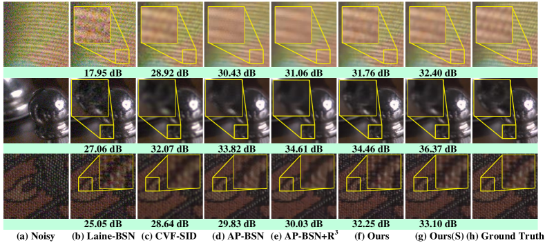
Figure 6: Quantitative comparisons on SIDD validation dataset.

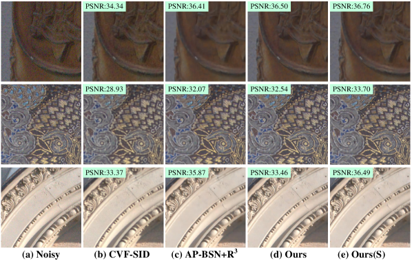
Figure 7: Quantitative comparisons on DND benchmark dataset.

5 Experiment

5.1 Experimental Configurations

Implementation Details.

We adapt Laine’s UNet-like BSN [24] as our network. We set $k=7$ and $k=1$ for training and inference, respectively. The input images are cropped into $128\times 128$ patches with a batch size of 8. The network is optimized with an Adam optimizers with a learning rate of $2\times 10^{-4}$ and $[\beta_{1},\beta_{2}]$ of $[0.9,0.999]$. We train the network for 60k iterations, and the learning rate is half-decayed per 10k iterations. For blind-spot self ensemble, we choose to average $k\in{\{0,1,3,5\}}$. All experiments are finished on an Nvidia RTX 3080.

Real-World Datasets. We train and evaluate our method on two well-known real-world image denoising datasets, Smartphone Image Denoising Dataset (SIDD) [1] and Darmstadt Noise Dataset (DND) [36]. SIDD-Medium training dataset consists of 320 clean-noisy pairs captured under various scenes and illuminations. Note that the SIDD online benchmark website is not accessible, so we adopt the SIDD validation dataset, containing 1280 noisy patches with a size of $256\times 256$ for validation and performance evaluation.

DND benchmark consists of 50 noisy images captured with consumer-grade cameras of various sensor sizes and does not provide clean images. DND dataset is captured under normal lighting conditions compared to the SIDD dataset, and therefore presenting less noise. We adopt widely-used peak signal-to-noise ratio (PSNR) and structural similarity (SSIM) metrics to evaluate our method.

5.2 Comparisons for Real-World Denoising

Quantitative Measure. Tab. I presents quantitative comparisons with other methods on the SIDD validation and DND benchmark datasets. We denote the distilled network as AT-BSN (S), where S means small and self-ensemble. Note that AT-BSN (S) is actually a Non-BSN despite its name. As a self-supervised algorithm, our method outperforms all existing unpaired and self-supervised methods, achieving state-of-the-art performance on both datasets. Our results without $\dagger$ marks indicate we employ the model trained on SIDD-Medium directly on the DND benchmark. These results show the generalization ability of our method. Note that results with $\dagger$ show the advantage of our fully self-supervised method. Furthermore, the results of AT-BSN (S) demonstrate the potential to enhance performance by integrating the advantages of different blind-spot sizes.

Qualitative Measure. Fig. 6 and Fig. 7 present the qualitative comparisons. It is evident that our method is capable of preserving the most texture details. As no downsampling process is used, no aliasing artifacts occur. In addition, using a smaller blind-spot size during inference minimizes information loss and maintains most image textures and spatial structure. On the other hand, AP-BSN without R³ shows obvious aliasing artifacts, while the images tend to be excessively smoothing with R³. Interestingly, if we set the blind-spot size $k$ to 1 during training, our method will degenerate into Laine’s BSN[24]. Such a network is found to learn an approximately identity mapping that is close to the noisy input itself, which indicates that highly spatial-correlated noise in real-world scenarios is challenging to classical self-supervised methods.

5.3 Complexity Analysis

We also present a comparison of our method with several recent methods in terms of inference time, the number of parameters, and computation cost. As shown in Tab. II, our method achieves the best performance while having the smallest amount of parameters. Furthermore, our AT-BSN (S) owns even fewer parameters, and since no rotation operation is required, the inference time is significantly reduced. Although CVF-SID owns little parameters, the final denoised results are restored by two successive CVF-SID models, leading to longer time consumption. We also found that the inference time of AP-BSN + R³ is significantly increased compared to AP-BSN, as it requires R³ post-process to eliminate the aliasing effect caused by downsampling. In contrast, our method does not suffer from the aliasing effect and does not require any post-processing.

TABLE II: Complexity Analysis. The multiplier-accumulator operations (MACs) and inference time are measured on $512\times 512$ patches from DND benchmark datasets.

Methods	Params↓	MACs↓	Time↓	PSNR↑
	(M)	(G)	(ms)	(dB)
CVF-SID (S2)[33]	1.19	311.44	106.2	34.81
AP-BSN[26]	3.66	838.92	78.6	35.49
AP-BSN $+$ R3[26]	3.66	7653.97	1168.4	36.48
AT-BSN (Ours)	1.12	560.06	28.2	36.64
AT-BSN (S) (Ours)	0.86	106.53	2.4	37.13

5.4 Analysis of Asymmetric Blind-Spots

We conduct an ablation study on the combination of different blind-spot sizes during training and inference to evaluate the effectiveness of the asymmetric blind-spots strategy and the robustness of our proposed method. Specifically, we performed experiments on the combinations of training blind-spot sizes $k_{a}\in\{5,7,9,11,13,15\}$ and inference blind-spot sizes $k_{b}\in\{0,1,3,5,7,9,11,13,15\}$, using AT-BSN trained on the SIDD validation dataset. The results are shown in Fig. 8.

According to Fig. 2, the noise spatial correlation of the SIDD dataset becomes negligible outside the $7\times 7$ patch. As a consequence, our method could achieve the best performance at $k_{a}=7$. In addition, although the combination of $k_{a}=7$ and $k_{b}=1$ achieved the best performance for inference, we found that our method exhibited robustness to different experimental groups. That is, during training, overly large blind-spot sizes present little impact on the final performance, and using slightly larger blind-spot sizes during inference also imposes few impact on the results. However, models trained with $k_{a}\leq 5$ perform poorly as the noise spatial correlation is not suppressed sufficiently.

We also note that the performance of AP-BSN sharply declined with the increase of the inference PD stride factor as reported in [26]. We attempted to explain this from the perspective of the ERFs [30]. As shown in Fig. 3, the ERF of AP-BSN mapped to the original image expands dramatically with the expansion of the PD stride factor, causing severe local information loss and resulting in significant aliasing artifacts. In contrast, our method only loses the central $k*k$ pixels and therefore exhibits relatively better robustness.

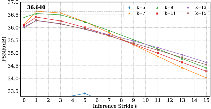
Figure 8: Ablation experiments on the combinations of different blind-spots between training and inference. Extreme values such as $k=15$ is also included. The results indicate that our method presents robustness in the selection of $k$.

6 Conclusion

In this paper, we propose a novel paradigm to break the spatial correlation of noise in real-world scenes while minimizing the disruption of global structure and high-frequency information, thus preserving fine-grained details. Specifically, we introduce a blind-spot network with tunable blind-spot sizes, which strikes a balance between suppressing noise spatial correlation and preserving local information by employing asymmetric blind-spots during training and inference. Furthermore, to better integrate the advantages of different blind-spot sizes, we propose blind-spot self-ensemble to improve performance. Additionally, we employ the output of the self-ensemble to distill a non-blind-spot network, further enhancing performance and reducing computational redundancy. The experimental results on the real-world noise datasets demonstrate the comprehensive superiority of our method in terms of performance, computational complexity, and inference time, achieving a new state-of-the-art in the self-supervised denoising field.

References

- [1] Abdelrahman Abdelhamed, Stephen Lin, and Michael S Brown. A high-quality denoising dataset for smartphone cameras. In CVPR, 2018.
- [2] Saeed Anwar and Nick Barnes. Real image denoising with feature attention. In ICCV, 2019.
- [3] Joshua Batson and Loic Royer. Noise2Self: Blind denoising by self-supervision. In ICML, 2019.
- [4] Benoit Brummer and Christophe De Vleeschouwer. Natural image noise dataset. In CVPR Workshops, 2019.
- [5] Harold C Burger, Christian J Schuler, and Stefan Harmeling. Image denoising: Can plain neural networks compete with bm3d? In CVPR, pages 2392–2399. IEEE, 2012.
- [6] Sungmin Cha, Taeeon Park, and Taesup Moon. GAN2GAN: Generative noise learning for blind image denoising with single noisy images. In ICLR, 2021.
- [7] A. Chambolle. An algorithm for total variation minimization and applications. Journal of Mathematical Imaging and Vision, 20:89–97, 2004.
- [8] Priyam Chatterjee, Neel Joshi, Sing Bing Kang, and Yasuyuki Matsushita. Noise suppression in low-light images through joint denoising and demosaicing. In CVPR, 2011.
- [9] Jingwen Chen, Jiawei Chen, Hongyang Chao, and Ming Yang. Image blind denoising with generative adversarial network based noise modeling. In CVPR, 2018.
- [10] Liang-Chieh Chen, George Papandreou, Florian Schroff, and Hartwig Adam. Rethinking atrous convolution for semantic image segmentation. arXiv:1706.05587, 2017.
- [11] Shen Cheng, Yuzhi Wang, Haibin Huang, Donghao Liu, Haoqiang Fan, and Shuaicheng Liu. NBNet: Noise basis learning for image denoising with subspace projection. In CVPR, 2021.
- [12] Kostadin Dabov, Alessandro Foi, Vladimir Katkovnik, and Karen Egiazarian. Image denoising by sparse 3-D transform-domain collaborative filtering. IEEE TIP, 16(8):2080–2095, 2007.
- [13] M. Elad and M. Aharon. Image denoising via sparse and redundant representations over learned dictionaries. TIP, 15:3736–3745, 2006.
- [14] Ian Goodfellow, Jean Pouget-Abadie, Mehdi Mirza, Bing Xu, David Warde-Farley, Sherjil Ozair, Aaron Courville, and Yoshua Bengio. Generative adversarial nets. In NIPS, 2014.
- [15] Shuhang Gu, Lei Zhang, Wangmeng Zuo, and Xiangchu Feng. Weighted nuclear norm minimization with application to image denoising. In CVPR, 2014.
- [16] Shi Guo, Zifei Yan, Kai Zhang, Wangmeng Zuo, and Lei Zhang. Toward convolutional blind denoising of real photographs. In CVPR, 2019.
- [17] Zhiwei Hong, Xiaocheng Fan, Tao Jiang, and Jianxing Feng. End-to-end unpaired image denoising with conditional adversarial networks. In AAAI, 2020.
- [18] Xiaowan Hu, Ruijun Ma, Zhihong Liu, Yuanhao Cai, Xiaole Zhao, Yulun Zhang, and Haoqian Wang. Pseudo 3D auto-correlation network for real image denoising. In CVPR, 2021.
- [19] Tao Huang, Songjiang Li, Xu Jia, Huchuan Lu, and Jianzhuang Liu. Neighbor2Neighbor: Self-supervised denoising from single noisy images. In CVPR, 2021.
- [20] Geonwoon Jang, Wooseok Lee, Sanghyun Son, and Kyoung Mu Lee. C2N: Practical generative noise modeling for real-world denoising. In ICCV, 2021.
- [21] Qiyu Jin, Gabriele Facciolo, and Jean-Michel Morel. A review of an old dilemma: Demosaicking first, or denoising first? In CVPR Workshops, 2020.
- [22] Yoonsik Kim, Jae Woong Soh, Gu Yong Park, and Nam Ik Cho. Transfer learning from synthetic to real-noise denoising with adaptive instance normalization. In CVPR, 2020.
- [23] Alexander Krull, Tim-Oliver Buchholz, and Florian Jug. Noise2Void-learning denoising from single noisy images. In CVPR, 2019.
- [24] Samuli Laine, Tero Karras, Jaakko Lehtinen, and Timo Aila. High-quality self-supervised deep image denoising. In NeurIPS, 2019.
- [25] Marc Lebrun, Miguel Colom, and Jean-Michel Morel. The noise clinic: a blind image denoising algorithm. Image Processing On Line, 5:1–54, 2015.
- [26] Wooseok Lee, Sanghyun Son, and Kyoung Mu Lee. Ap-bsn: Self-supervised denoising for real-world images via asymmetric pd and blind-spot network. In CVPR, pages 17725–17734, 2022.
- [27] Jaakko Lehtinen, Jacob Munkberg, Jon Hasselgren, Samuli Laine, Tero Karras, Miika Aittala, and Timo Aila. Noise2Noise: Learning image restoration without clean data. In ICML, 2018.
- [28] Pengju Liu, Hongzhi Zhang, Kai Zhang, Liang Lin, and Wangmeng Zuo. Multi-level Wavelet-CNN for image restoration. In CVPR Workshops, 2018.
- [29] Yang Liu, Zhenyue Qin, Saeed Anwar, Pan Ji, Dongwoo Kim, Sabrina Caldwell, and Tom Gedeon. Invertible denoising network: A light solution for real noise removal. In CVPR, pages 13365–13374, 2021.
- [30] Wenjie Luo, Yujia Li, Raquel Urtasun, and Richard Zemel. Understanding the effective receptive field in deep convolutional neural networks. NIPS, 29, 2016.
- [31] Ruijun Ma, Shuyi Li, Bob Zhang, and Zhengming Li. Generative adaptive convolutions for real-world noisy image denoising. In AAAI, volume 36, pages 1935–1943, 2022.
- [32] Nick Moran, Dan Schmidt, Yu Zhong, and Patrick Coady. Noisier2Noise: Learning to denoise from unpaired noisy data. In CVPR, 2020.
- [33] Reyhaneh Neshatavar, Mohsen Yavartanoo, Sanghyun Son, and Kyoung Mu Lee. Cvf-sid: Cyclic multi-variate function for self-supervised image denoising by disentangling noise from image. In CVPR, pages 17583–17591, 2022.
- [34] Tongyao Pang, Huan Zheng, Yuhui Quan, and Hui Ji. Recorrupted-to-Recorrupted: Unsupervised deep learning for image denoising. In CVPR, 2021.
- [35] Sung Hee Park, Hyung Suk Kim, Steven Lansel, Manu Parmar, and Brian A Wandell. A case for denoising before demosaicking color filter array data. In Asilomar Conference on Signals, Systems and Computers, 2009.
- [36] Tobias Plotz and Stefan Roth. Benchmarking denoising algorithms with real photographs. In CVPR, 2017.
- [37] Luminita A. Vese and S. Osher. Modeling textures with total variation minimization and oscillating patterns in image processing. Journal of Scientific Computing, 19:553–572, 2003.
- [38] Panqu Wang, Pengfei Chen, Ye Yuan, Ding Liu, Zehua Huang, Xiaodi Hou, and Garrison Cottrell. Understanding convolution for semantic segmentation. In WACV, pages 1451–1460. Ieee, 2018.
- [39] Zejin Wang, Jiazheng Liu, Guoqing Li, and Hua Han. Blind2unblind: Self-supervised image denoising with visible blind spots. In CVPR, pages 2027–2036, 2022.
- [40] Xiaohe Wu, Ming Liu, Yue Cao, Dongwei Ren, and Wangmeng Zuo. Unpaired learning of deep image denoising. In ECCV, 2020.
- [41] Jun Xu, Yuan Huang, Ming-Ming Cheng, Li Liu, Fan Zhu, Zhou Xu, and Ling Shao. Noisy-As-Clean: Learning self-supervised denoising from corrupted image. IEEE TIP, 29:9316–9329, 2020.
- [42] Jun Xu, Lei Zhang, David Zhang, and Xiangchu Feng. Multi-channel weighted nuclear norm minimization for real color image denoising. In ICCV, pages 1096–1104, 2017.
- [43] Fisher Yu and Vladlen Koltun. Multi-scale context aggregation by dilated convolutions. arXiv:1511.07122, 2015.
- [44] Zongsheng Yue, Hongwei Yong, Qian Zhao, Lei Zhang, and Deyu Meng. Variational denoising network: Toward blind noise modeling and removal. In NeurIPS, 2019.
- [45] Zongsheng Yue, Qian Zhao, Lei Zhang, and Deyu Meng. Dual adversarial network: Toward real-world noise removal and noise generation. In ECCV, 2020.
- [46] Kai Zhang, Wangmeng Zuo, Yunjin Chen, Deyu Meng, and Lei Zhang. Beyond a Gaussian denoiser: Residual learning of deep CNN for image denoising. IEEE TIP, 26(7):3142–3155, 2017.
- [47] Kai Zhang, Wangmeng Zuo, and Lei Zhang. FFDNet: Toward a fast and flexible solution for CNN-based image denoising. IEEE TIP, 27(9):4608–4622, 2018.
- [48] Yi Zhang, Dasong Li, Ka Lung Law, Xiaogang Wang, Hongwei Qin, and Hongsheng Li. Idr: Self-supervised image denoising via iterative data refinement. In CVPR, pages 2098–2107, June 2022.
- [49] Yuqian Zhou, Jianbo Jiao, Haibin Huang, Yang Wang, Jue Wang, Honghui Shi, and Thomas Huang. When AWGN-based denoiser meets real noises. In AAAI, 2020.