Supervised learning for table tennis match prediction

Abstract

Machine learning, classification and prediction models have applications across a range of fields. Sport analytics is an increasingly popular application, but most existing work is focused on automated refereeing in mainstream sports and injury prevention. Research on other sports, such as table tennis, has only recently started gaining more traction. This paper proposes the use of machine learning to predict the outcome of table tennis single matches. We use player and match statistics as features and evaluate their relative importance in an ablation study. In terms of models, a number of popular models were explored. We found that 5-fold cross-validation and hyperparameter tuning was crucial to improve model performance. We investigated different feature aggregation strategies in our ablation study to demonstrate the robustness of the models. Different models performed comparably, with the accuracy of the results (61-70%) matching state-of-the-art models in comparable sports, such as tennis. The results can serve as a baseline for future table tennis prediction models, and can feed back to prediction research in similar ball sports.

1 Introduction

Table tennis is a quick and highly technical sport, requiring players to respond to an incoming ball trajectory within milliseconds. Rallies are intense, with ball speeds of 60–70mph and rotational speeds of 9000rpm. The proximity between players is lower compared to similar sports such as tennis and badminton. The outcome of a game can be influenced by subtle factors, which can be hard for a human to recognize.

Machine learning methods have been used frequently in other sports, such as tennis and football. Proposed applications involve improved training efficiency as well as result prediction. Specifically, result prediction is of high concern to sport fans, but little has been done in table tennis prediction.

While manually-collected datasets alongside some analysis have been available in the past (Wang et al., 2019), it is only recent developments in multi-class event spotting and small object tracking that made accurate, detailed in-game data attainable. In this paper, we propose using some of this freshly available data to train and evaluate state-of-the-art classification algorithms on both men and women’s professional singles matches.

The paper is organized as follows: we first review relevant publications on sports prediction and describe the OSAI dataset on which our work is built. Then, we describe the proposed feature set. Finally, we evaluate and compare the performance of four different commonly used models and perform a feature ablation.

2 Background

Table tennis is played by hundreds of millions of people world-wide, with almost 40 000 professionals registered with the International Table Tennis Federation (ITTF). Games are fast-paced and highly technical, but there are factors that make it attractive for mathematical modelling: matches have only two possible outcomes (there are no draws).

A table tennis match consists of a sequence of sets; in a professional singles match, the first player to win best of seven sets wins the match. This paper will be looking at modelling professional singles matches only, thus there is no need to consider team line-ups. In a set, the first player that earns at least eleven points and at least two more than their opponent wins the set. Each player serves twice before alternating, however, if the score reaches at least 10-10, each player serves only once before alternating. The full set of rules are published by the ITTF (2022).

3 Related Work

3.1 Machine Learning

Machine learning (ML) is a branch of artificial intelligence that has been successfully applied to many areas of industry and science, including disease diagnosis in medicine (Kourou et al., 2015), pattern recognition (Weiss & Kapouleas, 1989), computer vision (Khan & Al-Habsi, 2020) and bioinformatics (Larranaga et al., 2006). The problem of predicting a table tennis match can be thought of as a supervised binary classification problem, with unambiguous ground-truth match outcome labels widely available.

3.2 ML in Sports

In the past, manual data collection methods for sports have typically proven time-consuming and prone to human error and bias. Recent improvements in data capture have sparked interest in automatic data collection and analysis for a range of sports. Xing et al. (2010) proposed a dual-mode two-way Bayesian inference approach to track multiple highly dynamic and interactive players from videos in team sports such as basketball, football and hockey. Claudino et al. (2019) used different ML methods, such as neural networks and decision tree classifiers, to investigate injury risk and performance in football, basketball, handball and volleyball. Davoodi & Khanteymoori (2010) used neural networks for horse racing prediction, where eight features were used as input nodes to each neural network. This included information such as horse weight and race distance, to predict the eventual finishing time and rank of every horse in a race.

Applications of ML in sports can help players and performance analysts in identifying critical factors that contribute to winning. Appropriate tactics can be identified in maximising player performance. Aside from formulating strategies to win matches, using machine learning methods for sport result prediction has become popular due to the expanding domain in betting (Bunker & Thabtah, 2019), which necessitates high predictive accuracy. Other applications include automated scouting and recruitment (Bunker & Thabtah, 2019) and umpiring assistance (Žemgulys et al., 2018).

3.3 Prediction in Tennis

A number of data-driven models are available for tennis. Clarke & Dyte (2000) predicted the outcome of professional tennis matches with 61–69% accuracy using player rating points. Mapping player ability to a single rank can fail to capture complex factors, especially when comparing lower-rated players. In our paper we consider more complex features.

Barnett & Clarke (2005) use rich historical data to predict the probability of a player winning a single point, building up a Markov chain to predict the winner of a match. The authors’ approach is compelling, but there is no published data on the accuracy of their model on a larger dataset.

Knottenbelt et al. (2012) proposed a common opponent model to find a pre-play estimate of winning a match. This was achieved by analysing match statistics for opponents that both players encountered in the past. The model computed the probability of each player winning a point on their serve, and hence the match. The authors found a 59–77% accuracy, with an estimated return on investment of 6.85% when put into the betting market for over four major tennis tournaments in 2011.

3.4 ML in Table tennis

In table tennis, ML research has focused so far on computer vision and automated data collection. Voeikov et al. (2020) proposed a neural network (TTNet) that allowed for real-time processing of high-resolution table tennis videos. They extract temporal and spatial data, such as ball detection and in-game events, potentially replacing manual data collection by sport scouts. The model can also assist referees. More recently, Zhang et al. (2010) used computer vision to allow a robot to play table tennis. They computed the 3D coordinates of a table tennis ball from a pair of video feeds to estimate the trajectory, the landing and striking point.

This paper builds on these existing works by utilising data by Voeikov et al. (2020), and applies it to the yet unexplored problem of supervised table tennis match prediction.

4 Dataset

The primary source of data are automatic captures from TTNet (Voeikov et al., 2020), released by OSAI (2020). We use Tokyo 2020 Olympics and Tischtennis-Bundesliga (German table tennis league) data, which include men and women’s singles matches. Potential features include player rank and in-match statistics such as percentage of points won on serve and receive, stroke and error types. Match progression can be plotted for each set, recording the location of each ball bounce (see Fig. 1).

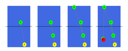
Figure 1: Progression of a rally demonstrating the landing point of each ball bounce. Yellow indicates service which starts a rally and red indicates an error ending the rally. Green indicates all other ball bounces. Based on data from OSAI (OSAI, 2020).

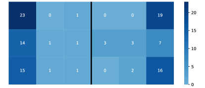
Figure 2: Location of the last bounce of the winning ball, summed over an example match. Each side of the table is split into nine equal parts.

To reduce the dimensionality of the problem, a rally can be represented as the location of the winning shot. Furthermore, each half of the table can be split into nine equal sections, and the location of winning shots can be grouped (Fig. 2). Further grouping can involve the number of forehands and the number of backhands used to win a point, or whether it was a ‘short’ or ‘long’ rally (Fig. 3). Samples with missing data entries were removed from the dataset.

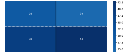
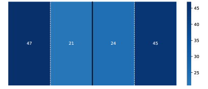
Figure 3: Number of points won by forehand vs. backhand (top); by a short vs. long rally (bottom) in an example match (OSAI, 2020).

One of the main challenges in constructing a successful result predictor is the selection of salient features. To address this, features were carefully hand-picked and evaluated in Section 6.

4.1 Match Representation

We represent each match ($i$) from a participating player’s ($P$) perspective as follows:

• a feature vector ($\underline{x}_{i}$) consisting of player and match statistics,

• the target variable ($y$), indicating the result of the match:

  $$y_{i}=\begin{cases}1,&\text{if $P$ wins}\\ -1,&\text{if $P$ loses}\end{cases}.$$ (1)

With incomplete matches removed from the dataset, there are no other possible outcomes (there are no draws in table tennis). Each match actually maps to two ($\underline{x_{i}}$,$y_{i}$) pairs, from the perspective of the two participating players.

4.2 Feature Engineering

An approach dictated by current state-of-the-art in tennis was used (Barnett & Clarke, 2005; Sipko & Knottenbelt, 2015; Cornman et al., 2017) to form new features for table tennis. These features are player-focused, as unlike in team sports, we do not need to consider line-ups, collective team ability or substitutions.

Table 1 shows the final set of features. Newly derived features are indicated with *. More detailed explanations can be found in the subsections below.

Table 1: Feature Summary

Feature	Explanation
SP	percentage of total points won on serve
RP	percentage of total points won on receive
LRP	percentage of total points won on a long rally
SRP	percentage of total points won on a short rally
FHP	percentage of total points won on a forehand
BHP	percentage of total points won on a backhand
RANK	player ranking
RANKDIFF*	difference in rank between opponents
SA*	player serve advantage
SRA*	player short rally advantage
FHA*	player forehand advantage
BALANCE*	measure of how well rounded a player is

SP: Serve Percentage

The proportion of points won on serve by a player. If the serve and error are made on opposing sides of the table, it was won by the serving player.

RP: Receive Percentage

The proportion of points won by the receiving player. E.g. in Fig. 1, the serve and error is made by the same player, so the point is won by the receiver.

LRP: Long Rally Percentage

The proportion of points won on a long rally by a player to the total number of rallies won. In this paper we define a long rally as a rally of at least five shots. E.g. Fig. 3 shows that one player won 47 points on a long rally, while the other won 45.

SRP: Short Rally Percentage

Compared to LRP, this is the proportion of points won on a short rally by a player. E.g. Fig. 3 shows that one player won 21 points on a short rally, while the other won 24 in the entire match.

FHP: Forehand Percentage

The proportion of points won on a forehand by a player, determined by the type of stroke used on the winning shot of a rally. Fig. 3 shows one player won 24 points on a forehand, and the other winning 38.

BHP: Backhand Percentage

The proportion of points won on a backhand by a player. Fig. 3 shows one player won 43 points on a backhand, and the other winning 29.

RANK

The ranking of the player by ITTF

RANKDIFF*: Rank Difference

$$\text{RANKDIFF}=\begin{cases}\text{RANK}_{a}-\text{RANK}_{b}&\text{for player $a$}\\ \text{RANK}_{b}-\text{RANK}_{a}&\text{for player $b$},\end{cases}$$ (2)

where RANK_a and RANK_b are player rankings for payers $a$ and $b$ at the time of the match. A rank advantage (i.e. lower numerical value than an opponent’s), yields a negative RANKDIFF. Rankings are mostly reliable for the top players; for example, players of rank 2 and 7 are more likely to have an accurate depiction of their relative ability than players of rank 150 and 155, despite the difference being identical. To account for this, we apply a simple non-linearity and set RANKDIFF to $0$ for matches where both players are ranked over 100.

SA*, SRA*, HA*

Serve advantage is calculated as the difference between their serve and receive winning percentage. This shows how likely a player is to win a point if they are serving rather than if they are on receive. Subsequently, the advantage a respective player has in a short rally over a long rally, as well as the advantage a respective player has in a forehand stroke over a backhand stroke, can be calculated.

BALANCE*

Players of a higher skill level tend to have fewer weaknesses and are stronger in more aspects of the game. We propose measuring the overall well-roundness as:

$$\textit{BALANCE}=\frac{|\textit{SA}|+|\textit{SRA}|+|\textit{FHA}|}{3}.$$ (3)

4.3 Feature Scaling

To account for the varying numerical range of the input features, and to make features comparable, we each input is standardized to a zero mean with a unit standard deviation.

4.4 Live vs. aggregate data

Each feature vector $\underline{x}_{i}$ represents a single match $i$ from a $P$ player’s perspective with several features observed during that game (SP, RP, LRP, SRP, FHP, VHP, SA*, SRA*, FHA*, BALANCE*). Predicting the outcome from all these features post-match is a trivial task; however, we postulate that the result of a match can be predicted from live in-match data well before the game ends, which is supported by the quick convergence of features as illustrated on an example match in Fig. 4. Hence, we fit our models on $(\underline{x}_{i},y_{i})$ pairs. We also validate the performance of these fitted models in Section 6.1 with the feature vector $\underline{x}_{i}$ averaged over all past and future matches of player $p$ except for the target match. This approach is not robust for novice players who have very few data points and whose performance might change rapidly. We hope to address this limitation in future work.

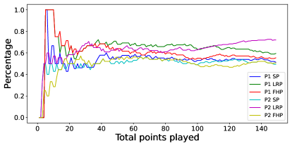
Figure 4: Illustration of how individual features stabilize after a relatively short time on an example match. P1 and P2 correspond to the perspective of the two participating players.

5 Models

Four ML models were evaluated (logistic regression, random forest, SVMs, MLPs) as implemented in Scikit-Learn (Pedregosa et al., 2011).

5.1 Logistic Regression

The logistic function maps the input feature $\underline{x}_{i}$ to a probability value $p_{i}$. Values over $0.5$ correspond to the player winning match $i$. Training minimizes the logistic loss function (Hazan et al., 2014):

$$(p)=-\frac{1}{n}\sum_{i=1}^{n}p_{i}\log\left(\frac{y_{i}+1}{2}\right)+(1-p_{i})\log\left(\frac{1-y_{i}}{2}\right),$$ (4)

where $n$ is number of matches, $p_{i}$ is the predicted probability of a player winning match $i$, and $y_{i}$ is as defined in Eq. 1.

5.2 Random Forest

Random forest classifiers consist of an ensemble of simpler decision trees $\{h(\underline{x},\theta_{k}),\ k=1,...\}$. For the $k$th tree, a random vector $\theta_{k}$ is generated and fitted to produce a classifier $h(\underline{x},\theta_{k})$ (Breiman, 2001). During inference, each tree casts a vote from input $\underline{x}$; the output is decided by a majority vote. Decision trees tend to be simpler to interpret and quicker to train.

5.3 Support Vector Machines (SVM)

SVMs have been used for tennis match predictions. These models identify the optimal hyperplane in the multi-dimensional feature space that separates data points into the two target classes (win, lose). During training, the marginal distance between this decision boundary and the instances closest to the boundary is maximized. SVMs have a choice of kernels, including linear, polynomial, sigmoid or a radial basis function (Cornman et al., 2017).

5.4 Multilayer Perceptron Neural Networks (MLP)

An MLP is an artificial neural network consisting of an input layer ($\underline{x}$), an output layer (prediction), and one or more hidden layers in-between. Neurons in consecutive layers are connected (no connections within layers) (Noriega, 2005). Each connection has an associated weight. Training an MLP involves adjustments of these weights using backpropagation to minimize the difference between model output and the desired output.

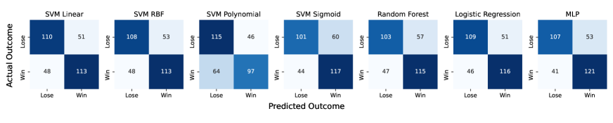
Figure 5: Confusion matrices comparing the predicted and actual outcomes of test cases for each trained model.

5.5 Evaluating Models

To compare the performance of different model predictions, we calculated the accuracy of each model

$$\text{accuracy}=\frac{tp+tn}{tp+tn+fp+fn},$$ (5)

where $tp$ and $tn$ are true positives and true negatives, and $fp$ and $fn$ are false positives and false negatives respectively.

To get a more balanced idea about model performance, we also compute F1 scores as:

$$\text{precision}=\frac{tp}{tp+fp}\quad\text{recall}=\frac{tp}{tp+fn}$$ (6)

$$F1=\frac{2\times\text{precision}\times\text{recall}}{\text{precision}+\text{recall}},$$ (7)

which is effectively an F measure with $\beta=1$ (Sokolova et al., 2006). During training, the model can over-fit to a specific dataset, which reduces model robustness. In cross validation, the dataset is split into $k$ random subsets, known as folds, and one is selected as a test set for the model to test on, while the others are used as a training set for the model to train on. This is repeated $k$ times where a different subset of data is used as the test set each time, and the overall performance of the model is calculated as the average of accuracy scores for each iteration (Berrar, 2019). For model fitting here, 5-fold cross validation was used: the dataset was split in training:validation:test in a 72:18:10 ratio. 10% of the original dataset was kept as a test set to validate hyperparameter tuning. The remaining 90% of data was split in an 80:20 ratio for the 5-fold training; 80% to train the model, 20% to optimize hyperparameters.

5.6 Hyperparameter Tuning

We used a brute-force grid search to fine tune parameters of the model that are outside the usual training domain (hyperparameters) e.g. the number of trees in a random forest classifier. The best combination of hyperparameters for a model is determined by whichever has the highest accuracy on the validation set using 5-fold cross validation.

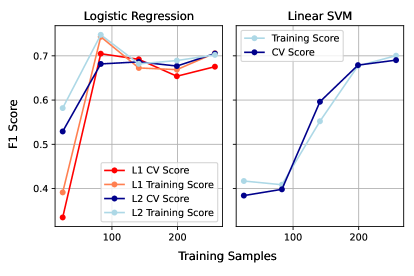
Figure 6: Logistic regression and linear kernel SVM learning curves. The difference in F1 score for L1 and L2 regularisation is also illustrated.

For logistic regression, the type of solver, penalty function and the $C$ terms value were adjusted. $C$ is a regularisation term; the lower the value of $C$, the stronger the effect of regularisation. We found that $C=1.0$, and ‘liblinear’ solver resulted in the best average accuracy. In terms of regularisation, L2 regularisation gave better results than L1 (Fig. 6).

For SVMs, the two main hyperparameters that were adjusted were the kernel type and penalty value $C$. Using a linear kernel and $C=0.2$ gave the highest F1 score on the test set compared to other kernels. The learning curve for an SVM model using a linear kernel is shown in Fig. 6.

6 Experimental Results

Table 2: Model performance comparing validation and test sets before hyperparameter tuning

Model	Validation set		Test set
	Acc	F1	Acc	F1
Logistic Regression	0.696$\pm{0.025}$	0.701$\pm{0.025}$	0.694	0.645
Random Forest	0.658$\pm{0.018}$	0.658$\pm{0.028}$	0.639	0.667
Support Vector Machine
$\rightarrow$ Linear	0.680$\pm{0.019}$	0.679$\pm{0.030}$	0.611	0.611
$\rightarrow$ RBF	0.680$\pm{0.022}$	0.681$\pm{0.029}$	0.611	0.611
$\rightarrow$ Polynomial	0.677$\pm{0.009}$	0.669$\pm{0.017}$	0.556	0.563
$\rightarrow$ Sigmoid	0.590$\pm{0.022}$	0.553$\pm{0.028}$	0.694	0.579
MLP Neural Network	0.686$\pm{0.013}$	0.707$\pm{0.016}$	0.583	0.634

Table 3: Model performance comparing validation and test sets after hyperparameter tuning

Model	Validation set		Test set
	Acc	F1	Acc	F1
Logistic Regression	0.699$\pm{0.024}$	0.705$\pm{0.023}$	0.722	0.706
Random Forest	0.677$\pm{0.032}$	0.688$\pm{0.033}$	0.667	0.684
Support Vector Machine
$\rightarrow$ Linear	0.696$\pm{0.029}$	0.690$\pm{0.035}$	0.639	0.629
$\rightarrow$ RBF	0.700$\pm{0.025}$	0.677$\pm{0.034}$	0.667	0.600
$\rightarrow$ Polynomial	0.705$\pm{0.021}$	0.685$\pm{0.021}$	0.611	0.563
$\rightarrow$ Sigmoid	0.705$\pm{0.017}$	0.690$\pm{0.019}$	0.694	0.621
MLP Neural Network	0.696$\pm{0.019}$	0.708$\pm{0.020}$	0.694	0.703

The main results are reported in Table 3 and Fig. 5. Both accuracy and F1 score are reported for the validation and test sets. The standard error for each score for the validation set is reported as a basis of defining uncertainty. The validation column shows that most models perform comparably with approx. 70% accuracy. This value is also comparable to state-of-the-art metrics in tennis match prediction. Table 2 also indicates results across models before hyperparameter tuning (parameters will be set to default values), so that the difference can be compared.

F1 scores indicate that MLP Neural Networks (with a relu activation) slightly over-perform their competitors, but the difference is not significant. The hidden layer size was set to 2 and the maximum number of iterations the solver iterates was chosen to be 200. The solver for weight optimization is set to ‘lbfgs’, a quasi-Newton optimizer. The learning rate for scheduling weight updates is set to constant. However, the generic layered structure of a neural network has proven to be time consuming. Additionally, this technique is considered a ‘black box’ technology, and finding out why a neural network has outstanding or even poor performance is difficult (Noriega, 2005).

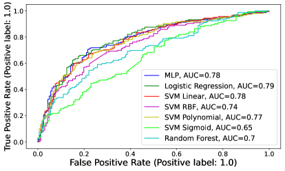
Figure 7: ROC Learning Curves for the overall performance of each model.

Receiving operating characteristics (ROC, Fig. 7) support the quantitative results. The kernel choice for SVM models makes a noticeable difference; the areas under the ROC curves are otherwise comparable for all other models.

One qualitative advantage of using a random forest classifier is its training speed, which made hyperparameter tuning easier. The maximum number of levels in each decision tree was set to 80, the maximum number of features considered for splitting a node was set to 4, the minimum number of data points allowed in a leaf node was set to 4 and the number of trees that were in the classifier was set to 200.

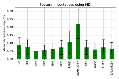
Figure 8: Importance of features from random forest classifier based on Gini impurity. In our dataset, RANKDIFF appears to be the most important feature.

Another significant advantage of a random forest classifier is that the importance of features can also be extracted and visualized. Fig. 8 shows this as the mean decrease in Gini impurity for features across all trees. The impurity of a node is the probability of a specific feature being classified incorrectly assuming that it is selected randomly (Cassidy & Deviney, 2014).

6.1 Ablation Study

Fig. 8 predicts that the most important feature in a random forest model is RANKDIFF, which justifies the inclusion of hand-crafted features. To reinforce this finding, we computed the accuracy and F1 score for each model with and without the derived features. All scores are lower for models that do not use newly derived features, and the accuracy score is significantly lower in SVMs compared to other models. See Table 4.

Table 4: Model performance with and without newly derived features

Model	With		Without
	Acc	F1	Acc	F1
Logistic Regression	0.699	0.705	0.631	0.668
Random Forest	0.677	0.688	0.661	0.673
Support Vector Machine
$\rightarrow$ Linear	0.696	0.690	0.556	0.619
$\rightarrow$ RBF	0.700	0.677	0.500	0.591
$\rightarrow$ Polynomial	0.705	0.685	0.500	0.640
$\rightarrow$ Sigmoid	0.705	0.690	0.472	0.642
MLP Neural Network	0.696	0.708	0.639	0.683

A more real-world benchmark of performance is to understand how well the model can predict the outcome of a match before, without having seen that match. We computed accuracy and F1 scores for this scenario by restricting the model input to aggregate feature vectors $\underline{x_{i}^{\prime}}$ which contain the average features from all past and future matches, but exclude the target match $x_{i}$ itself. Table 5 shows similar results to live prediction, with accuracy values of 61–67%. This indicates that our model is unlikely to have overfitted and just learnt existing match results and that it could be used as a robust match predictor.

Table 5: Model performance with the target match removed from the aggregate input features

Model	Test set
	Acc	F1
Logistic Regression	0.639	0.667
Random Forest	0.667	0.714
Support Vector Machine
$\rightarrow$ Linear	0.639	0.667
$\rightarrow$ RBF	0.639	0.649
$\rightarrow$ Polynomial	0.611	0.632
$\rightarrow$ Sigmoid	0.639	0.649
MLP Neural Network	0.667	0.714

7 Conclusion and Future Work

This paper explores how supervised classification models can be used to predict the results of table tennis matches. The original dataset was retrieved from OSAI (OSAI, 2020).

This paper utilises existing models as implemented in Scikit-learn (logistic regression, random forest classification, SVMs, multi-layer perceptrons); our contribution lies in applying these using 5-fold cross-validation and hyperparameter tuning to the problem of table tennis match prediction. We also propose using a handful of engineered features, from which a non-linear rank difference has been proved to be the most salient in our ablation study. To investigate overfitting, We consider aggregating feature across all matches of a player including or excluding the target match and demonstrate that our model performs comparably in both cases. T

Our results are comparable to the accuracy of state-of-the-art tennis prediction models (approx. 70% accuracy). Following hyperparameter tuning, the difference between models was often modest. Other considerations when picking a model for similar applications could include training time or model transparency (at both of which random forests excel).

Future work could explore combining TTNet with our prediction model to provide live match predictions. It would be also interesting quantifying uncertainty and to test against real betting odds. As automated table tennis analytics are becoming available below professional leagues, the authors are also interested whether the importance of features and the model choice transfers to these matches as well.

References

- (1)
- Barnett & Clarke (2005) Barnett, T. & Clarke, S. R. (2005), ‘Combining player statistics to predict outcomes of tennis matches’, IMA Journal of Management Mathematics 16(2), 113–120.
- Berrar (2019) Berrar, D. (2019), ‘Cross-validation.’.
- Breiman (2001) Breiman, L. (2001), ‘Random forests’, Machine learning 45(1), 5–32.
- Bunker & Thabtah (2019) Bunker, R. P. & Thabtah, F. (2019), ‘A machine learning framework for sport result prediction’, Applied computing and informatics 15(1), 27–33.
- Cassidy & Deviney (2014) Cassidy, A. P. & Deviney, F. A. (2014), Calculating feature importance in data streams with concept drift using online random forest, in ‘2014 IEEE International Conference on Big Data (Big Data)’, IEEE, pp. 23–28.
- Clarke & Dyte (2000) Clarke, S. R. & Dyte, D. (2000), ‘Using official ratings to simulate major tennis tournaments’, International transactions in operational research 7(6), 585–594.
- Claudino et al. (2019) Claudino, J. G., Capanema, D. d. O., de Souza, T. V., Serrão, J. C., Machado Pereira, A. C. & Nassis, G. P. (2019), ‘Current approaches to the use of artificial intelligence for injury risk assessment and performance prediction in team sports: a systematic review’, Sports medicine-open 5(1), 1–12.
- Cornman et al. (2017) Cornman, A., Spellman, G. & Wright, D. (2017), ‘Machine learning for professional tennis match prediction and betting’, Stanford Unverisity .
- Davoodi & Khanteymoori (2010) Davoodi, E. & Khanteymoori, A. R. (2010), ‘Horse racing prediction using artificial neural networks’, Recent Advances in Neural Networks, Fuzzy Systems & Evolutionary Computing 2010, 155–160.
- Hazan et al. (2014) Hazan, E., Koren, T. & Levy, K. Y. (2014), Logistic regression: Tight bounds for stochastic and online optimization, in ‘Conference on Learning Theory’, PMLR, pp. 197–209.
- ITTF (2022) ITTF (2022), ‘Ittf handbook’, https://documents.ittf.sport/document/284. Accessed: 2022-05-03.
- Khan & Al-Habsi (2020) Khan, A. I. & Al-Habsi, S. (2020), ‘Machine learning in computer vision’, Procedia Computer Science 167, 1444–1451.
- Knottenbelt et al. (2012) Knottenbelt, W. J., Spanias, D. & Madurska, A. M. (2012), ‘A common-opponent stochastic model for predicting the outcome of professional tennis matches’, Computers & Mathematics with Applications 64(12), 3820–3827.
- Kourou et al. (2015) Kourou, K., Exarchos, T. P., Exarchos, K. P., Karamouzis, M. V. & Fotiadis, D. I. (2015), ‘Machine learning applications in cancer prognosis and prediction’, Computational and structural biotechnology journal 13, 8–17.
- Larranaga et al. (2006) Larranaga, P., Calvo, B., Santana, R., Bielza, C., Galdiano, J., Inza, I., Lozano, J. A., Armananzas, R., Santafé, G., Pérez, A. et al. (2006), ‘Machine learning in bioinformatics’, Briefings in bioinformatics 7(1), 86–112.
- Noriega (2005) Noriega, L. (2005), ‘Multilayer perceptron tutorial’, School of Computing. Staffordshire University .
- OSAI (2020) OSAI (2020), ‘Osai’, https://osai.ai/. Accessed: 2022-01-18.
- Pedregosa et al. (2011) Pedregosa, F., Varoquaux, G., Gramfort, A., Michel, V., Thirion, B., Grisel, O., Blondel, M., Prettenhofer, P., Weiss, R., Dubourg, V. et al. (2011), ‘Scikit-learn: Machine learning in python’, the Journal of machine Learning research 12, 2825–2830.
- Sipko & Knottenbelt (2015) Sipko, M. & Knottenbelt, W. (2015), ‘Machine learning for the prediction of professional tennis matches’, MEng computing-final year project, Imperial College London .
- Sokolova et al. (2006) Sokolova, M., Japkowicz, N. & Szpakowicz, S. (2006), Beyond accuracy, f-score and roc: a family of discriminant measures for performance evaluation, in ‘Australasian joint conference on artificial intelligence’, Springer, pp. 1015–1021.
- Voeikov et al. (2020) Voeikov, R., Falaleev, N. & Baikulov, R. (2020), Ttnet: Real-time temporal and spatial video analysis of table tennis, in ‘Proceedings of the IEEE/CVF Conference on Computer Vision and Pattern Recognition Workshops’, pp. 884–885.
- Wang et al. (2019) Wang, J., Zhao, K., Deng, D., Cao, A., Xie, X., Zhou, Z., Zhang, H. & Wu, Y. (2019), ‘Tac-simur: Tactic-based simulative visual analytics of table tennis’, IEEE transactions on visualization and computer graphics 26(1), 407–417.
- Weiss & Kapouleas (1989) Weiss, S. M. & Kapouleas, I. (1989), An empirical comparison of pattern recognition, neural nets, and machine learning classification methods., in ‘IJCAI’, Vol. 89, Citeseer, pp. 781–787.
- Xing et al. (2010) Xing, J., Ai, H., Liu, L. & Lao, S. (2010), ‘Multiple player tracking in sports video: A dual-mode two-way bayesian inference approach with progressive observation modeling’, IEEE Transactions on Image Processing 20(6), 1652–1667.
- Žemgulys et al. (2018) Žemgulys, J., Raudonis, V., Maskeliūnas, R. & Damaševičius, R. (2018), ‘Recognition of basketball referee signals from videos using histogram of oriented gradients (hog) and support vector machine (svm)’, Procedia computer science 130, 953–960.
- Zhang et al. (2010) Zhang, Z., Xu, D. & Tan, M. (2010), ‘Visual measurement and prediction of ball trajectory for table tennis robot’, IEEE Transactions on Instrumentation and Measurement 59(12), 3195–3205.