Fast radio burst energy function in the presence of ${\rm DM}_{\rm host}$ variation

Abstract

Fast radio bursts (FRBs) have been found in great numbers but the physical mechanism of these sources is still a mystery. The redshift evolutions of the FRB energy distribution function and the volumetric rate shed light on revealing the origin of the FRBs. However, such estimations rely on the dispersion measurement (DM)–redshift ($z$) relationship. A few of FRBs detected recently show large excess DM beyond the expectation from the cosmological and Milky Way contributions, which indicates large spread of DM from their host galaxies. In this work, we adopt the lognormal distributed ${\rm DM}_{\rm host}$ model and estimate the energy function using the non-repeating FRBs selected from the Canadian Hydrogen Intensity Mapping Experiment (CHIME)/FRB Catalog 1. By comparing the lognormal distributed ${\rm DM}_{\rm host}$ model to the constant ${\rm DM}_{\rm host}$ model, the FRB energy function results are consistent within the measurement uncertainty. We also estimate the volumetric rate of the non-repeating FRBs in three different redshift bins. The volumetric rate shows that the trend is consistent with the stellar-mass density redshift evolution. Since the lognormal distributed ${\rm DM}_{\rm host}$ model increases the measurement errors, the inference of FRBs tracking the stellar-mass density is nonetheless undermined.

1 Introduction

The fast radio bursts (FRBs) are bright, violent flashes of radio emission with durations of the order of milliseconds. In 2007, the first FRB event was discovered by Lorimer et al. (2007) from the archived data of the Parkes telescope in Australia. Since then, a couple of FRB events were discovered by different radio telescopes, e.g., the Green Bank Telescope (GBT) and the Arecibo radio telescope. Chatterjee et al. (2017) for the first time confirmed the host galaxy of one FRB, i.e., FRB121102, which was discovered by the Arecibo radio telescope (Spitler et al., 2014). Recently, more than 800 FRBs are discovered by the advanced radio telescopes, such as the Canadian Hydrogen Intensity Mapping Experiment (CHIME), the Australian Square Kilometre Array Pathfinder (ASKAP), etc. Most of the FRBs are non-repeating events and dozens of sources are repeating bursts. Currently, only 21 of the FRBs are localized. In the future, it is expected that a large number of FRBs can be localized, and these localized FRBs have the potential to be developed into a powerful cosmological probe (Zhao et al., 2020; Qiu et al., 2022; Wu et al., 2022; Zhao et al., 2022a).

There is still an open question for the origin of FRBs. A series of theoretical models have been proposed to explain the FRB origin (Platts et al., 2019). Accurate localizations of FRBs give us hints about the origin of FRBs. In 2020, the Galactic magnetar SGR J1935+2154 (Bochenek et al., 2020; CHIME/FRB Collaboration et al., 2021) was found to produce an FRB that coincided in time with a non-thermal X-ray burst from the magnetar. It supports the conjecture that some FRBs may be produced by magnetars. The repeating FRB 20200120E is localized at the position of a globular cluster in M81 (Bhardwaj et al., 2021). Globular clusters are usually composed of old stars with low metal content, so this FRB source requires an old population as the progenitor. By contrast, the repeating FRB 20201124A is localized to a massive, star-forming galaxy (Fong et al., 2021) at the redshift of $z=0.098$ (Nimmo et al., 2022). However, only a small number of localized events are actually inadequate to reveal the origin of FRBs.

The FRB energy function is also an effective way to constrain the origin models of FRBs (James et al., 2022; Zhang et al., 2021; Luo et al., 2020). The energy functions allow us to study the redshift evolution of volumetric rate of FRBs. If the origin of FRBs is related to young stellar populations, the volumetric FRB rate should increase with increasing redshift, as the density of cosmic star formation rate increases towards higher redshift, up to $z$ $\sim$ 2. Conversely, if FRB progenitors are old, such as white dwarfs, neutron stars or black holes, the volumetric rate follows the evolution of stellar mass, i.e. it should decrease towards higher redshift. Hashimoto et al. (2020) found that the number density of non-repeating FRB sources does not show any significant redshift evolution, which is consistent with the evolution of stellar mass in the universe. In their recent research, Hashimoto et al. (2022) reported that neutron stars and black holes are more likely to be the progenitors of non-repeating FRBs.

Recently, a few of FRBs show large excess DM beyond the expectation from the cosmological and Milky Way contributions (Spitler et al., 2014; Chatterjee et al., 2017; Hardy et al., 2017; Tendulkar et al., 2017; Chittidi et al., 2021). In particular, Niu et al. (2022) reported a detection of FRB 190520B with ${\rm DM}_{{\rm host}}\approx 903^{+72}_{-111}\,{\rm pc}\,{\rm cm}^{-3}$, which is almost an order of magnitude higher than the average ${\rm DM}_{\rm host}$ of the FRBs discovered so far. We summarize the values of ${\rm DM}_{\rm obs}$ and ${\rm DM}_{\rm host}$ of all the localized FRBs in Table 1. In this work, we study the effect of ${\rm DM}_{\rm host}$ uncertainty on the FRB energy function estimation, as well as the redshift evolution of FRB event rate. Note that, in this work, the Planck 2018 $\Lambda$ cold dark matter model is adopted as a fiducial model, with the best-fit cosmological parameters $H_{0}=67.36$ km s^-1 Mpc^-1, $\Omega_{\rm b}=0.0493$, $\Omega_{\rm m}=0.3153$, and $\Omega_{\Lambda}=0.6847$.

Table 1: ${\rm DM}_{\rm obs}$ and ${\rm DM}_{{\rm host}}$ of the localized FRBs.

${\rm ID}$	${\rm DM}_{\rm obs}\,[{\rm pc}\,{\rm cm}^{-3}]$	$z$	${\rm DM}_{{\rm host}}\,[{\rm pc}\,{\rm cm}^{-3}]$
FRB20121102A	557.000	0.1927	41.921690
FRB20180301A	536.000	0.3305	37.579857
FRB20180916B	348.800	0.0337	48.369933
FRB20180924B	362.160	0.3212	37.838656
FRB20181112A	589.000	0.4755	33.886818
FRB20190102C	364.545	0.2913	38.720669
FRB20190523A	760.800	0.6600	30.120482
FRB20190608B	340.050	0.1178	44.730721
FRB20190611B	332.630	0.3778	36.289737
FRB20190711A	592.600	0.5217	32.857988
FRB20190714A	504.130	0.2365	40.436717
FRB20191001A	506.920	0.2340	40.518639
FRB20191228A	297.500	0.2432	40.218790
FRB20200120E	87.820	0.0008	50.007001
FRB20200430A	380.250	0.1608	43.073742
FRB20200906A	577.800	0.3688	36.528346
FRB20201124A	412.000	0.0979	45.541488
FRB20220610A	1457.600	1.0160	1304.00000
FRB20190520B	1204.700	0.2400	903.000000
FRB20210405L	565.170	0.6600	21.000000
FRB20190614D	959.000	0.6000	57.000000

This paper is organized as follows; In Section 2, we describe the FRB catalogue, as well as the selection criteria, used in this work. The Bayesian framework used for the redshift estimation is described in Section 3. In Section 4, we present the energy functions and volumetric rates of non-repeating FRB sources along with their redshift evolution. The conclusions are presented in Section 5.

2 Data

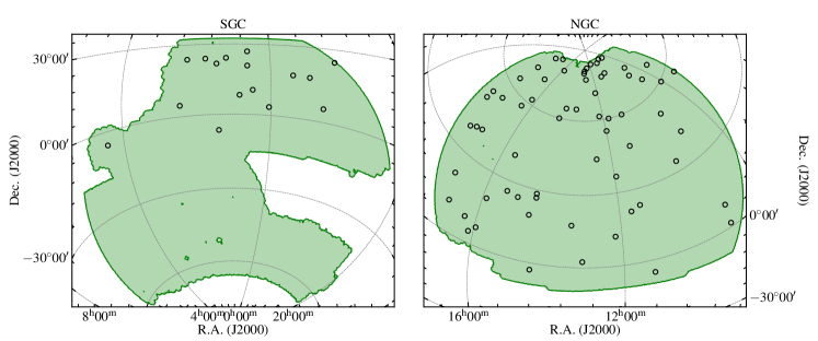
Figure 1: The sky locations of the selected FRBs. The footprint of the galaxy sample used in this work is shown with the green area and the FRBs are shown with the black circles.

2.1 FRB catalog

We use the first release of CHIME/FRB Catalog 1 (CHIME/FRB Collaboration et al., 2021), which contains 474 non-repeating bursts and 62 repeating bursts from $18$ repeaters. The $536$ burst events were detected between from 2018 July 25 to 2019 July 1 over an effective survey duration of $214.8$ days. In order to minimize the selection effects, a number of criteria are suggested (Shin et al., 2022; Hashimoto et al., 2022).

1. Events with bonsai_snr $<10$ are rejected, where bonsai_snr is the signal-to-noise ratio (S/N) recorded in the catalog. Shin et al. (2022) suggests S/N cut of $12$ since signal below ${\rm S/N}=12$ may be misclassified as radio-frequency interference (RFI). In this work, we use the bursts with S/N over $10$, which maintains a meaningful number of FRB samples for the statistical analysis (Hashimoto et al., 2022).

2. Events with ${\rm DM}_{\rm obs}<1.5\times{\rm max}\left({\rm DM}_{\rm NE2001},{\rm DM}_{\rm YMW16}\right)$ are rejected to ensure extragalactic origin of the events. ${\rm DM}_{\rm obs}$ is the measured DM; ${\rm DM}_{\rm NE2001}$ and ${\rm DM}_{\rm YMW16}$ are the DM of the Milky Way estimated according to the NE2001 model (Cordes & Lazio, 2002) and the YMW16 model (Yao et al., 2017), respectively.

3. Events with $\log_{10}\left(\tau_{\rm scat}/{\rm ms}\right)>0.8$ are rejected, where $\tau_{\rm scat}$ is the scattering timescale.

4. Events with $\log_{10}\left(F_{\nu}/{\rm Jy\,ms}\right)<0.5$ are rejected, where $F_{\nu}$ is the fluence of the burst.

5. Events detected in the side lobes of the telescope primary beam are rejected.

After applying the selection criteria, we have $176$ FRB events selected, including $12$ repeaters.

Previous analysis with the mock data shows that a significant fraction of FRBs are missed by the CHIME detection algorithm, i.e., only 39638 out of 84697 injected mock events are detected (Shin et al., 2022). The total number of events needs to be scaled according to the detection fraction,

$$N_{\rm FRB}=N_{\rm obs}\times\frac{\num{84697}}{\num{39638}}.$$ (1)

In addition, the fraction of missed events also depend on the property of the FRB signal. Longer scattering times or lower fluencies result in a higher number of missed events. Following Hashimoto et al. (2022), the relationship between the observed and intrinsic data distributions is described by

$$P(\vartheta)=P_{\rm obs}(\vartheta)\times s(\vartheta)^{-1},$$ (2)

where $P(\vartheta)$ and $P_{\rm obs}(\vartheta)$ represent the intrinsic and observed distributions of the FRB property $\vartheta$, respectively. $s(\vartheta)$ is the selection function as a function of different FRB properties. The properties considered for deriving the selection function include the dispersion measure (${\rm DM}_{\rm obs}$), scattering timescale ($\tau_{\rm scat}$), intrinsic duration ($w_{\rm int}$) and fluence ($F_{\nu}$); see CHIME/FRB Collaboration et al. (2021) for details. We adopt the best-fit selection functions in Hashimoto et al. (2022),

$$s({\rm DM}_{\rm obs})= - 0.7707(\log_{10}{\rm DM}_{\rm obs})^{2}$$ (3)

$$+ 4.5601(\log_{10}{\rm DM}_{\rm obs})-5.6291,$$

$$s(\tau_{\rm scat})= - 0.2922(\log_{10}\tau_{\rm scat})^{2}$$ (4)

$$- 1.0196(\log_{10}\tau_{\rm scat})+1.4592,$$

$$s(w_{\rm int})= - 0.0785(\log_{10}w_{\rm int})^{2}$$ (5)

$$- 0.5435(\log_{10}w_{\rm int})+0.9574,$$

$$\log_{10}s(F_{\nu})= 1.7173(1-\exp(-2.0348\log_{10}F_{\nu}))$$ (6)

$$- 1.7173.$$

The sky locations of the selected FRBs are shown in Figure 1 with the black circles.

2.2 Galaxy catalog

In order to evaluate the redshifts of the unlocalized FRBs, we follow the method developed in Zhao et al. (2022b), which actually employs the dark siren method in gravitational wave cosmology (Del Pozzo, 2012; Wang et al., 2022; Song et al., 2022). It assumes that an FRB always locates in a galaxy and the redshift of the FRB can be statistically estimated by associating the FRB event with its potential host galaxies according to a underlying galaxy catalogue.

In this work, we adopt the galaxy catalogue from Dark Energy Spectroscopic Instrument (DESI) Legacy Surveys. The Legacy Surveys combine three imaging projects of different telescopes, i.e. the Beijing-Arizona Sky Survey (BASS, Zou et al., 2017), the Dark Energy Camera Legacy Survey (DECaLS, Flaugher et al., 2015), and the Mayall z-band Legacy Survey (MzLS, Silva et al., 2016), covering about $\num{14000}\,{\rm deg}^{2}$ of the northern hemisphere and producing the target catalog for the DESI survey; for an overview of the Legacy Surveys, see Dey et al. (2019). We use the galaxy sample from the $8$-th public data release of the Legacy Surveys, i.e., the Data Release $8$ (DR8). The spectroscopic redshift of the galaxy sample is substituted for the photometric redshift, if available, in accordance with the sample selection process in Yang et al. (2021). In total, there are 129.35 million galaxies remaining in the galaxy sample. The footprint of the galaxy sample is illustrated with the green area in Figure 1, where the galaxies locating in the South Galactic Cap (SGC) and the North Galactic Cap (NGC) are shown in the left and right panels, respectively.

3 Methods

3.1 Bayesian framework

We adopt a Bayesian data analysis scheme to measure the FRBs’ redshifts. The Bayesian inference relates the probability density functions (PDFs) involving data and parameters,

$$P(\vartheta|x)\propto P(\vartheta)P(x|\vartheta),$$ (7)

where $P(x|\vartheta)$ is the likelihood function of the data given the model parameters and $P(\vartheta|x)$ is the posterior PDF, i.e. the PDF of the parameters given the data set. In this work, we shall estimate the posterior PDF of the FRBs’ redshifts $z$ given the measurement set of DM,

$$P(z|{\rm DM})\propto P(z)P({\rm DM}|z),$$ (8)

where $P({\rm DM}|z)$ represents the likelihood function of the measured DM given the parameter set. The measured DM is the combination of several components,

$${\rm DM}={\rm DM}_{{\rm MW}}+{\rm DM}_{{\rm halo}}+{\rm DM}_{{\rm IGM}}+\frac{{\rm DM}_{{\rm host}}}{1+z},$$ (9)

where the contributions are from the interstellar medium of the Milky Way (${\rm DM}_{{\rm MW}}$), the ionized gas in the local halo (${\rm DM}_{{\rm halo}}$), the intergalactic medium (${\rm DM}_{{\rm IGM}}$), and the FRB host galaxy (${\rm DM}_{{\rm host}}$).

${\rm DM}_{{\rm MW}}$ and ${\rm DM}_{{\rm halo}}$ can be subtracted according to the current model. The CHIME/FRB catalogue provides the dispersion measure with the Milky Way contribution subtracted using the NE2001 model (Cordes & Lazio, 2002) and the YMW16 model (Yao et al., 2017), respectively. We test both of the two different models and find no significant difference in the final estimation. In the following analysis, only the results with the YMW16 model are presented.

The precise contribution of the local halo to DM is uncertain. Yamasaki & Totani (2019) provides the prediction of ${\rm DM}_{{\rm halo}}$ with a mean value of $43\,{\rm pc}\,{\rm cm}^{-3}$ and a full range of $30\sim 245\,{\rm pc}\,{\rm cm}^{-3}$. We adopt the mean value of $43\,{\rm pc}\,{\rm cm}^{-3}$ in the following analysis.

After subtracting ${\rm DM}_{{\rm MW}}$ and ${\rm DM}_{{\rm halo}}$ for the total ${\rm DM}$, the measurement likelihood function is written as

$$P({\rm DM}|z)=\int {\rm d} {\rm DM}_{{\rm host}}\,{\rm d}\,{\rm DM}_{{\rm IGM}}\,P({\rm DM}|{\rm DM}_{{\rm host}},{\rm DM}_{{\rm IGM}},z)$$ (10)

$$\times P({\rm DM}_{{\rm host}}|z)P({\rm DM}_{{\rm IGM}}|z),$$

where $P({\rm DM}_{{\rm host}}|z)$ and $P({\rm DM}_{{\rm IGM}}|z)$ are the likelihood functions of ${\rm DM}_{{\rm host}}$ and ${\rm DM}_{{\rm IGM}}$, respectively, and the integration represents the marginalization of ${\rm DM}_{{\rm host}}$ and ${\rm DM}_{{\rm IGM}}$ likelihood function.

3.2 $P({\rm DM}_{{\rm IGM}}|z)$

The DM contribution from the IGM (${\rm DM}_{{\rm IGM}}$) can be explained as the dispersion induced when an FRB is emitted at a random point in the universe of redshift $z$ and propagates to $z=0$. The average value of ${\rm DM}_{{\rm IGM}}$ at redshift $z$ is given by the integration of the free electron number density $n_{\rm e}$ along the line of sight,

$$\langle{\rm DM}_{{\rm IGM}}\rangle=\int_{0}^{z}{\rm d}z^{\prime}\frac{n_{\rm e}(z^{\prime})}{1+z^{\prime}}\left(\frac{1}{1+z^{\prime}}\frac{c}{H_{0}}\frac{1}{E(z^{\prime})}\right),$$ (11)

where $H_{0}$ is the Hubble constant. In this work, we consider the standard flat $\Lambda$CDM model $E(z)=\sqrt{\Omega_{\rm m}(1+z)^{3}+\Omega_{\Lambda}}$. Assuming the universe is fully ionized at $z\lesssim 3$, the free electron number density equals to the total electron number density,

$$n_{\rm e}(z)=f_{{\rm IGM}}\bar{\rho}_{{\rm b},0}(1+z)^{3}\left(\frac{Y_{\rm H}\chi_{{\rm e},{\rm H}}(z)}{m_{\rm p}}+2\frac{Y_{\rm He}\chi_{{\rm e},{\rm He}}(z)}{4m_{\rm p}}\right),$$ (12)

where the $Y_{\rm H}\sim 3/4$ and $Y_{\rm He}\sim 1/4$ denote the primordial mass fractions of hydrogen and helium, respectively. The ionization fraction, $\chi_{{\rm e},{\rm H}}(z)$ and $\chi_{{\rm e},{\rm He}}(z)$ for hydrogen and helium, are both set to unity at the redshift of $z\lesssim 2$ (Fan et al., 2006; McQuinn et al., 2009). $\bar{\rho}_{{\rm b},0}=3H_{0}^{2}\Omega_{\rm b}/8\pi G$ is the comoving cosmological baryon density at current epoch, $m_{\rm p}$ is the mass of proton and $f_{{\rm IGM}}=0.83$ represents the fraction of the free electrons in the IGM (Deng & Zhang, 2014).

The ${\rm DM}_{{\rm IGM}}$ deviation from $\langle{\rm DM}_{{\rm IGM}}\rangle$ is expected to follow the normal distribution. Thus, the likelihood function is expressed as

$$P({\rm DM}_{{\rm IGM}}|z)=\frac{1}{\mathcal{N}_{{\rm IGM}}}\exp\left(-\frac{1}{2}\frac{\left({\rm DM}_{\rm IGM}-\langle\mathrm{DM}_{\mathrm{IGM}}\rangle\right)^{2}}{\sigma^{2}_{{\rm IGM}}}\right),$$ (13)

where $\mathcal{N}_{{\rm IGM}}=\sigma_{{\rm IGM}}\sqrt{2\pi}$ is the normalization factor and $\sigma_{{\rm IGM}}=173.8\,z^{0.4}\,{\rm pc}\,{\rm cm}^{-3}$ (Qiang & Wei, 2021).

3.3 $P({\rm DM}_{{\rm host}}|z)$

The major uncertainty of the FRB redshift measurement comes from the variation of the DM contribution from the FRB’s host galaxy. A few of FRBs show large excess DM beyond the expectation from the the cosmological and Milky Way contributions (Spitler et al., 2014; Chatterjee et al., 2017; Hardy et al., 2017; Tendulkar et al., 2017; Chittidi et al., 2021). Recently, Niu et al. (2022) reported a detection of FRB 190520B with ${\rm DM}_{{\rm host}}\approx 903^{+72}_{-111}\,{\rm pc}\,{\rm cm}^{-3}$, which is almost an order of magnitude higher than the average ${\rm DM}_{\rm host}$ of the FRBs discovered so far. Generally, the large spread of the ${\rm DM}_{\rm host}$ can be modeled using a lognormal distribution and the corresponding likelihood function is expressed as

$$P({\rm DM}_{\rm host}|z)=\frac{1}{{\mathcal{N}}_{{\rm host}}}\exp\left(-\frac{1}{2}\frac{\left(\ln x-\mu\right)^{2}}{\sigma^{2}_{{\rm host}}}\right),$$ (14)

where $x={{\rm DM}_{\rm host}}\big{/}{{\rm pc}\,{\rm cm}^{-3}}$, ${\mathcal{N}}_{{\rm host}}=x\sigma_{{\rm host}}\sqrt{2\pi}$ is the normalization factor, $\mu$ and $\sigma_{\rm host}$ are the lognormal distribution parameters. Using the cosmological magnetohydrodynamical simulation, Zhang et al. (2020) (hereinafter referred to as the Zhang20 model) provided the fitting results,

$$\mu=\ln\left(32.97(1+z)^{0.84}\right),\,\,\sigma_{\rm host}=1.248.$$ (15)

In addition, Mo et al. (2022) proposed another detailed analysis for the distribution of the ${\rm DM}_{\rm host}$ for different FRB population models. In this work, we adopt the fitting results of

$$\mu=\ln(63.55),\,\,\sigma_{\rm host}=1.25,$$ (16)

from Mo et al. (2022) (hereinafter referred to as the Mo22 model). We compare the result differences between using such two ${\rm DM}_{\rm host}$ distribution models, as well as using the model of assuming constant ${\rm DM}_{\rm host}=50\,{\rm pc}\,{\rm cm}^{-3}$.

3.4 The posterior distribution of the FRB redshift

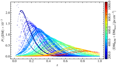
Figure 2: The redshift posterior probability distribution of each FRB event. Each curve represents the posterior probability of one FRB using the DESI Legacy Surveys DR8 galaxies’ redshift sample that located in the sky area determined by Equation (18). The colors of the lines indicate the values of ${\rm DM}_{\rm IGM}+{\rm DM}_{\rm host}$.

The DM measurement likelihood function is expressed as

$$P({\rm DM}|{\rm DM}_{\rm host},{\rm DM}_{\rm IGM},z)=\frac{1}{\mathcal{N}}\exp\left(-\frac{1}{2}\frac{({\rm DM}-\Theta)^{2}}{\sigma^{2}_{{\rm DM}}}\right),$$ (17)

where $\mathcal{N}=\sigma_{\rm DM}\sqrt{2\pi}$ is the normalization factor, $\sigma_{\rm DM}$ is the measurement uncertainty and $\Theta={\rm DM}_{\rm host}+{\rm DM}_{\rm IGM}+{\rm DM}_{\rm MW}+{\rm DM}_{\rm halo}$ represents the DM’s theoretical value. Substituting Equations (13), (14) and (17) into Equation (10), we can estimate the posterior probability at a given redshift. Assuming the FRBs always locate in the galaxies, we shall use the redshifts of the galaxy catalog, i.e. the DESI Legacy Surveys DR8 catalog, as the prior distribution. For a given FRB, we use the redshifts of all the galaxies with their celestial coordinate $\alpha$ (Right ascension) and $\delta$ (Declination),

$$|\alpha_{\rm gal}-\alpha_{\rm FRB}|<\theta_{\alpha}\times\cos(\delta_{\rm FRB}),\,\,\,|\delta_{\rm gal}-\delta_{\rm FRB}|<\theta_{\delta},$$ (18)

where $\theta_{\alpha}$ and $\theta_{\delta}$ are the $68\%$ confidence pointing errors of the CHIME beam in the Right ascension and Declination direction, respectively. The estimated redshift posterior probabilities are shown in Figure 2. Each curve represents the posterior probability of one FRB using the DESI Legacy Surveys DR8 galaxies’ redshift sample locating in the sky area determined by Equation (18). The color of the curve indicates the value of ${\rm DM}_{\rm IGM}+{\rm DM}_{\rm host}$ of the FRB event. There is a clear trend that the FRB with larger DM has the posterior probability distribution peaking at higher redshift. This is consistent with the Macquart relation (Macquart et al., 2020). However, the posterior probability also shows a wide range of distribution, which indicates the large uncertainty of the redshift estimation. Such large uncertainty is dominated by the large scattering of ${\rm DM}_{\rm host}$.

3.5 Energy function

The FRB fluence ($F_{\nu}$) is converted to rest-frame isotropic radio energy ($E$) for each FRB via (Macquart & Ekers, 2018)

$$E=\frac{4\pi d_{\rm L}^{2}}{(1+z)^{2+\alpha}}F_{\nu}\Delta\nu,$$ (19)

where $d_{\rm L}$ is the luminosity distance to the FRB, $\alpha$ is the spectrum index of the FRB’s power-law spectrum across the frequencies and $\Delta\nu$ is the burst bandwidth. The burst bandwidth is calculated by high_freq$-$low_freq in the CHIME/FRB catalog, where high_freq and low_freq represent the upper and lower bands of the detection at full-width tenth-maximum (FWTM) (CHIME/FRB Collaboration et al., 2021).

The FRB energy function represents the number density of FRB events as a function of energy. The number density per unit time is estimated via each of the FRB event detection,

$${\rho}_{\rm obs}=\frac{1}{V_{\rm max}f_{\rm sky}\left(t_{\rm obs}/(1+z)\right)},$$ (20)

where $f_{\rm sky}=3\times 10^{-3}$ is the fraction of the sky covered by the CHIME’s field of view, $t_{\rm obs}=0.59\,{\rm yr}$ is the survey time for the first CHIME/FRB catalog and the factor of $1+z$ converts the survey time to the rest frame. $V_{\rm max}$ is defined as the flux limited maximum volume within which the FRB event could still be detected (Schmidt, 1968; Avni & Bahcall, 1980),

$$V_{\rm max}=\frac{4\pi}{3}\left(\chi_{\rm max}^{3}-\chi_{\rm min}^{3}\right),$$ (21)

where $\chi_{\rm min}$ and $\chi_{\rm max}$ are the comoving distances at the minimum and maximum redshifts. We adopt $z_{\rm min}=0.05$ in this work and $z_{\rm max}$ is estimated according the fluence of the FRB,

$$F_{\nu}=\frac{E(1+z_{\rm max})^{2+\alpha}}{4\pi d_{{\rm L},z_{\rm max}}^{2}\Delta\nu}>10^{0.5}\,{\rm Jy}\,{\rm ms}.$$ (22)

The number density estimated with Equation (19) needs to be corrected for the selection effect as mentioned in Section 2.1. Considering the selection function of Equations (3)–(6), the corrected number density is (Hashimoto et al., 2022)

$$\rho_{\rm corr}=\frac{1}{\mathcal{N}_{s}}W\rho_{\rm obs},$$ (23)

where $W=\big{(}s({\rm DM}_{\rm obs})s(\tau_{\rm scat})s(w_{\rm int})s(F_{\nu})\big{)}^{-1}$. $\mathcal{N}_{s}=\sum_{i}W_{i}/{N_{\rm FRB}}$ is the normalization factor, where $i$ denotes the $i$-th FRB event and $N_{\rm FRB}$ is the corrected total number, i.e., Equation (1).

We divide the full energy range occupied by the FRB detection into a number of energy bins ($\phi_{j}$) in the logarithmic scale and sum $\rho_{\rm corr}$ within each energy bin,

$$\phi_{j}=\frac{1}{\Delta_{j}\log_{10}E}\sum_{i}\rho_{{\rm corr},i},$$ (24)

where $\Delta_{j}\log_{10}E$ is the $j$-th energy bin size.

We perform a Monte Carlo (MC) simulation with $\num{10000}$ realizations of the redshift sample following the posterior probability distribution of Equation (10). The energy function is estimated using each of the realization. The estimation uncertainty is evaluated via the the standard deviation.

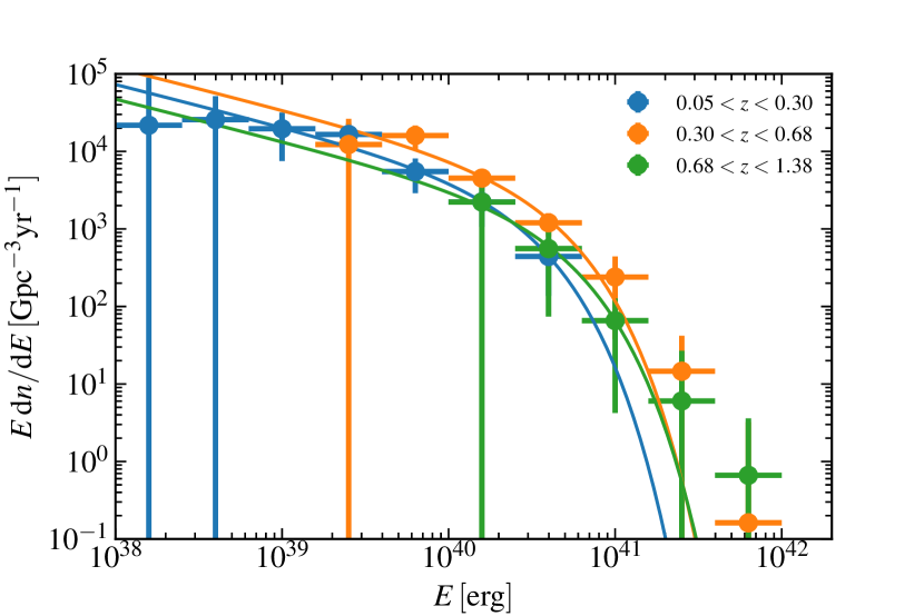
Figure 3: The energy functions of non-repeating CHIME FRB sources using Mo22 model. The results for three redshift bins are shown with three different colors. The best-fit Schechter functions are shown with solid lines.

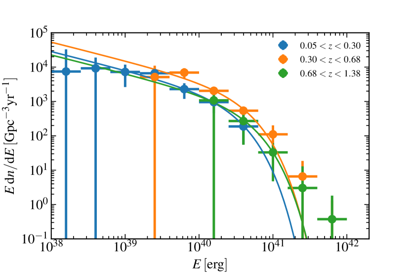
Figure 4: The energy functions of non-repeating CHIME FRB sources using Zhang20 Model. The results for three redshift bins are shown with three different colors. The best-fit Schechter functions are shown with solid lines.

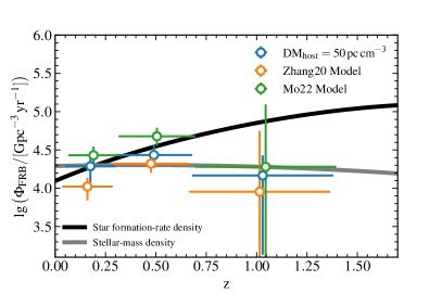
Figure 5: The volumetric rate of CHIME non-repeating FRBs as a function of redshift. The horizontal errors represent the redshift bin width and the vertical errors are the estimation uncertainty, which are estimated by 10000 times of the MC simulation. The results of the constant ${\rm DM}_{\rm host}$ model, the Zhang20 model, and the Mo22 model are shown with different colors.

4 Results and discussions

Figures 4 and 4 show the energy functions estimated using the CHIME/FRB catalog. The energy functions are estimated within three redshift bins, i.e. $0.05<z\leqslant 0.3$, $0.3<z\leqslant 0.68$ and $0.68<z\leqslant 1.38$ (follow Ref. (Hashimoto et al., 2022)). The estimated energy distribution functions of different redshift bins are shown in different colors. The results with different ${\rm DM}_{\rm host}$ models, i.e. the Mo22 model and the Zhang20 model, are shown in Figures 4 and 4, respectively.

The FRB energy distribution is modeled with a Schechter function (Schechter, 1976),

$$\phi(\lg E)\,{\rm d}\lg E=\phi^{\star}\left(\frac{E}{E^{\star}}\right)^{\gamma+1}\exp\left(-\frac{E}{E^{\star}}\right){\rm d}\lg E,$$ (25)

where $\phi^{\star}$ is the normalization factor, $\gamma+1$ is the faint-end slope and $E^{\star}$ is the break energy of the Schechter function. The energy distribution functions are fit to the measurements using the public package emcee (Foreman-Mackey et al., 2013). We use $\phi^{\star}$, $E^{\star}$ and $\gamma$ as the free parameters for the first redshift bin, i.e. $0.05<z<0.30$. Due to the lack of FRB data in the higher reshift bins, we only use $\phi^{\star}$ and $E^{\star}$ as the free parameters in the rest two redshift bins and fix $\gamma$ to the best-fit value of the first redshift bin.

Table 2: The fit values of parameters in Schechter function for FRB energy function.

	$\lg E^{\star}$	$\lg\phi^{\star}$	$\gamma$	$\lg\Phi$
$0.05<z<0.30$
Constant ${\rm DM}_{\rm host}$	$40.000_{-0.363}^{+0.428}$	$3.994_{-0.626}^{+0.254}$	$-1.046_{-0.373}^{+0.516}$	$4.277_{-0.301}^{+0.139}$
Zhang20 Model	$40.219_{-0.378}^{+0.592}$	$3.418_{-0.877}^{+0.358}$	$-1.382_{-0.224}^{+0.572}$	$4.035_{-0.192}^{+0.125}$
Mo22 Model	$40.225_{-0.382}^{+0.589}$	$3.783_{-0.882}^{+0.369}$	$-1.427_{-0.238}^{+0.537}$	$4.438_{-0.181}^{+0.121}$
$0.30<z<0.68$
Constant ${\rm DM}_{\rm host}$	$40.239_{-0.119}^{+0.169}$	$4.097_{-0.222}^{+0.164}$	–	$4.434_{-0.167}^{+0.129}$
Zhang20 Model	$40.503_{-0.150}^{+0.177}$	$3.370_{-0.226}^{+0.207}$	–	$4.321_{-0.116}^{+0.113}$
Mo22 Model	$40.496_{-0.153}^{+0.183}$	$3.729_{-0.235}^{+0.211}$	–	$4.678_{-0.123}^{+0.111}$
$0.68<z<1.38$
Constant ${\rm DM}_{\rm host}$	$40.408_{-0.451}^{+0.216}$	$3.772_{-0.847}^{+0.336}$	–	$4.167_{-1.033}^{+0.263}$
Zhang20 Model	$40.553_{-1.549}^{+0.461}$	$2.970_{-0.470}^{+1.640}$	–	$3.956_{-1.869}^{+0.794}$
Mo22 Model	$40.547_{-1.519}^{+0.534}$	$3.295_{-0.003}^{+2.204}$	–	$4.280_{-1.992}^{+0.813}$

The best-fit energy distribution function at each redshift bin is shown with the smooth curve in Figure 4 and Figure 4, respectively. The energy function estimated in each redshift bin is consistent with each other. There is no significant redshift evolution for using either the Mo22 model or the Zhang20 model. The fit values of the parameters in Equation (25) are list in Table 2. The volumetric rate of the FRBs is estimated by integrating the energy function within the available energy range of each redshift bin. The corresponding volumetric rates estimated using the best-fit energy functions are list in the last column of Table 2 and also shown in Figure 5. In Figure 5, the blue error bars show the FRB volumetric rates estimated by assuming a constant ${\rm DM}_{\rm host}=50\,{\rm pc}\,{\rm cm}^{-3}$, while the orange and green error bars show the results using ${\rm DM}_{\rm host}$ from the Zhang20 model and the Mo22 model, respectively. The horizontal error bars indicate the redshift bin width and the vertical error bars show the standard deviation. The solid black and gray curves show the cases of the star formation rate and the stellar-mass density, which are estimated using the fitting functions in Hashimoto et al. (2020). Both of the two curves are normalized for their amplitudes at redshift $z=0.2$ to the same value as the FRB volumetric rates estimated using the constant ${\rm DM}_{\rm host}$.

With the constant ${\rm DM}_{\rm host}$ assumption, the FRB volumetric rate shows the same trend as the stellar-mass density, which is consistent with the previous analysis (Hashimoto et al., 2022). By releasing the constant ${\rm DM}_{\rm host}$ assumption, the estimation uncertainty increases, especially for the high redshift bin. Within the estimation error, there is no significant difference between using and not using the constant ${\rm DM}_{\rm host}$ assumption. However, it can be obviously seen that the variation of ${\rm DM}_{\rm host}$ weakens the conclusion that the volumetric rate is consistent with the stellar-mass density. It is expected that the future much larger FRB and galaxy samples could greatly improve the measurement and draw a more solid conclusion.

5 Conclusions

In this work, we estimate the energy function and the volumetric rate of the non-repeating FRBs using CHIME/FRB Catalog 1. We follow the FRB selection criteria as used in the literature (Shin et al., 2022; Hashimoto et al., 2022). In the meanwhile, we follow the Bayesian framework data analysis scheme developed in Zhao et al. (2022b) and adopt the galaxy catalogue from Dark Energy Spectroscopic Instrument (DESI) Legacy Surveys to evaluate the redshift of the unlocalized FRBs.

We also consider different ${\rm DM}_{\rm host}$ models, including the model of constant ${\rm DM}_{\rm host}=50\,{\rm pc}\,{\rm cm}^{-3}$ and the lognormal distribution model, which are constrained using the magnetohydrodynamical simulation. Zhang et al. (2020) and Mo et al. (2022) both provided the fitting functions according to magnetohydrodynamical simulation (the Zhang20 and Mo22 models). The FRB energy function is estimated with each of the ${\rm DM}_{\rm host}$ model.

The Schechter function-like energy function model is considered and is fit to the measurements using the non-repeating FRBs from CHIME/FRB Catalog 1. The fit values of parameters are summarized in Table 2. We do not find significant difference between using the constant ${\rm DM}_{\rm host}$ model and the lognormal ${\rm DM}_{\rm host}$ models (i.e. the Zhang20 and Mo22 models).

We also estimate the FRB volumetric rate according to the best-fit energy distribution function and compare the trend of redshift evolution with the star formation-rate density and the stellar-mass density. We find that, with the lognormal ${\rm DM}_{\rm host}$ model, the estimation uncertainties increase. The trend of redshift evolution is consistent with the stellar-mass density for both the constant ${\rm DM}_{\rm host}$ model and the lognormal ${\rm DM}_{\rm host}$ models. However, since the lognormal distributed ${\rm DM}_{\rm host}$ model increases the measurement errors, the inference of FRBs tracking the stellar-mass density is nonetheless undermined. The measurement can be further improved in the future by using a larger FRB catalog and/or a deeper galaxy survey catalogue.

References

- Avni & Bahcall (1980) Avni, Y., & Bahcall, J. N. 1980, ApJ, 235, 694, doi: 10.1086/157673
- Bhardwaj et al. (2021) Bhardwaj, M., et al. 2021, Astrophys. J. Lett., 910, L18, doi: 10.3847/2041-8213/abeaa6
- Bochenek et al. (2020) Bochenek, C. D., Ravi, V., Belov, K. V., et al. 2020, Nature, 587, 59, doi: 10.1038/s41586-020-2872-x
- Chatterjee et al. (2017) Chatterjee, S., et al. 2017, Nature, 541, 58, doi: 10.1038/nature20797
- CHIME/FRB Collaboration et al. (2021) CHIME/FRB Collaboration, Amiri, M., et al. 2021, Astrophys. J. Supp., 257, 59, doi: 10.3847/1538-4365/ac33ab
- Chittidi et al. (2021) Chittidi, J. S., Simha, S., Mannings, A., et al. 2021, ApJ, 922, 173, doi: 10.3847/1538-4357/ac2818
- Cordes & Lazio (2002) Cordes, J. M., & Lazio, T. J. W. 2002. https://arxiv.org/abs/astro-ph/0207156
- Del Pozzo (2012) Del Pozzo, W. 2012, Phys. Rev. D, 86, 043011, doi: 10.1103/PhysRevD.86.043011
- Deng & Zhang (2014) Deng, W., & Zhang, B. 2014, Astrophys. J. Lett., 783, L35, doi: 10.1088/2041-8205/783/2/L35
- Dey et al. (2019) Dey, A., Schlegel, D. J., Lang, D., et al. 2019, AJ, 157, 168, doi: 10.3847/1538-3881/ab089d
- Fan et al. (2006) Fan, X.-H., Carilli, C. L., & Keating, B. G. 2006, Ann. Rev. Astron. Astrophys., 44, 415, doi: 10.1146/annurev.astro.44.051905.092514
- Flaugher et al. (2015) Flaugher, B., Diehl, H. T., Honscheid, K., et al. 2015, AJ, 150, 150, doi: 10.1088/0004-6256/150/5/150
- Fong et al. (2021) Fong, W.-f., et al. 2021, Astrophys. J. Lett., 919, L23, doi: 10.3847/2041-8213/ac242b
- Foreman-Mackey et al. (2013) Foreman-Mackey, D., Hogg, D. W., Lang, D., & Goodman, J. 2013, PASP, 125, 306, doi: 10.1086/670067
- Hardy et al. (2017) Hardy, L. K., et al. 2017, Mon. Not. Roy. Astron. Soc., 472, 2800, doi: 10.1093/mnras/stx2153
- Hashimoto et al. (2020) Hashimoto, T., Goto, T., On, A. Y. L., et al. 2020, Mon. Not. Roy. Astron. Soc., 498, 3927, doi: 10.1093/mnras/staa2490
- Hashimoto et al. (2022) Hashimoto, T., et al. 2022, Mon. Not. Roy. Astron. Soc., 511, 1961, doi: 10.1093/mnras/stac065
- James et al. (2022) James, C. W., Prochaska, J. X., Macquart, J. P., et al. 2022, Mon. Not. Roy. Astron. Soc., 510, L18, doi: 10.1093/mnrasl/slab117
- Lorimer et al. (2007) Lorimer, D. R., Bailes, M., McLaughlin, M. A., Narkevic, D. J., & Crawford, F. 2007, Science, 318, 777, doi: 10.1126/science.1147532
- Luo et al. (2020) Luo, R., Men, Y., Lee, K., et al. 2020, Mon. Not. Roy. Astron. Soc., 494, 665, doi: 10.1093/mnras/staa704
- Macquart & Ekers (2018) Macquart, J.-P., & Ekers, R. 2018, Mon. Not. Roy. Astron. Soc., 480, 4211, doi: 10.1093/mnras/sty2083
- Macquart et al. (2020) Macquart, J. P., et al. 2020, Nature, 581, 391, doi: 10.1038/s41586-020-2300-2
- McQuinn et al. (2009) McQuinn, M., Lidz, A., Zaldarriaga, M., et al. 2009, Astrophys. J., 694, 842, doi: 10.1088/0004-637X/694/2/842
- Mo et al. (2022) Mo, J.-F., Zhu, W., Wang, Y., Tang, L., & Feng, L.-L. 2022, Mon. Not. Roy. Astron. Soc., 518, 539, doi: 10.1093/mnras/stac3104
- Nimmo et al. (2022) Nimmo, K., et al. 2022, Astrophys. J. Lett., 927, L3, doi: 10.3847/2041-8213/ac540f
- Niu et al. (2022) Niu, C. H., et al. 2022, Nature, 606, 873, doi: 10.1038/s41586-022-04755-5
- Platts et al. (2019) Platts, E., Weltman, A., Walters, A., et al. 2019, Phys. Rept., 821, 1, doi: 10.1016/j.physrep.2019.06.003
- Qiang & Wei (2021) Qiang, D.-C., & Wei, H. 2021, Phys. Rev. D, 103, 083536, doi: 10.1103/PhysRevD.103.083536
- Qiu et al. (2022) Qiu, X.-W., Zhao, Z.-W., Wang, L.-F., Zhang, J.-F., & Zhang, X. 2022, JCAP, 02, 006, doi: 10.1088/1475-7516/2022/02/006
- Schechter (1976) Schechter, P. 1976, ApJ, 203, 297, doi: 10.1086/154079
- Schmidt (1968) Schmidt, M. 1968, Astrophys. J., 151, 393, doi: 10.1086/149446
- Shin et al. (2022) Shin, K., et al. 2022. https://arxiv.org/abs/2207.14316
- Silva et al. (2016) Silva, D. R., Blum, R. D., Allen, L., et al. 2016, in American Astronomical Society Meeting Abstracts, Vol. 228, American Astronomical Society Meeting Abstracts #228, 317.02
- Song et al. (2022) Song, J.-Y., Wang, L.-F., Li, Y., et al. 2022. https://arxiv.org/abs/2212.00531
- Spitler et al. (2014) Spitler, L. G., et al. 2014, Astrophys. J., 790, 101, doi: 10.1088/0004-637X/790/2/101
- Tendulkar et al. (2017) Tendulkar, S. P., et al. 2017, Astrophys. J. Lett., 834, L7, doi: 10.3847/2041-8213/834/2/L7
- Wang et al. (2022) Wang, L.-F., Shao, Y., Zhang, G.-P., Zhang, J.-F., & Zhang, X. 2022. https://arxiv.org/abs/2201.00607
- Wu et al. (2022) Wu, P.-J., Shao, Y., Jin, S.-J., & Zhang, X. 2022. https://arxiv.org/abs/2202.09726
- Yamasaki & Totani (2019) Yamasaki, S., & Totani, T. 2019, doi: 10.3847/1538-4357/ab58c4
- Yang et al. (2021) Yang, X., et al. 2021, Astrophys. J., 909, 143, doi: 10.3847/1538-4357/abddb2
- Yao et al. (2017) Yao, J. M., Manchester, R. N., & Wang, N. 2017, The Astrophysical Journal, 835, 29, doi: 10.3847/1538-4357/835/1/29
- Zhang et al. (2020) Zhang, G. Q., Yu, H., He, J. H., & Wang, F. Y. 2020, Astrophys. J., 900, 170, doi: 10.3847/1538-4357/abaa4a
- Zhang et al. (2021) Zhang, R. C., Zhang, B., Li, Y., & Lorimer, D. R. 2021, Mon. Not. Roy. Astron. Soc., 501, 157, doi: 10.1093/mnras/staa3537
- Zhao et al. (2020) Zhao, Z.-W., Li, Z.-X., Qi, J.-Z., et al. 2020, Astrophys. J., 903, 83, doi: 10.3847/1538-4357/abb8ce
- Zhao et al. (2022a) Zhao, Z.-W., Wang, L.-F., Zhang, J.-G., Zhang, J.-F., & Zhang, X. 2022a. https://arxiv.org/abs/2210.07162
- Zhao et al. (2022b) Zhao, Z.-W., Zhang, J.-G., Li, Y., et al. 2022b. https://arxiv.org/abs/2212.13433
- Zou et al. (2017) Zou, H., Zhou, X., Fan, X., et al. 2017, PASP, 129, 064101, doi: 10.1088/1538-3873/aa65ba