Safe Zeroth-Order Optimization Using Quadratic Local Approximations

Abstract

This paper addresses black-box smooth optimization problems, where the objective and constraint functions are not explicitly known but can be queried. The main goal of this work is to generate a sequence of feasible points converging towards a KKT primal-dual pair. Assuming to have prior knowledge on the smoothness of the unknown objective and constraints, we propose a novel zeroth-order method that iteratively computes quadratic approximations of the constraint functions, constructs local feasible sets and optimizes over them. Under some mild assumptions, we prove that this method returns an $\eta$-KKT pair (a property reflecting how close a primal-dual pair is to the exact KKT condition) within $O({1}/{\eta^{2}})$ iterations. Moreover, we numerically show that our method can achieve faster convergence compared with some state-of-the-art zeroth-order approaches. The effectiveness of the proposed approach is also illustrated by applying it to nonconvex optimization problems in optimal control and power system operation.

1 Introduction

Applications ranging from power network operations [1], machine learning [2] and trajectory optimization [3] to optimal control [4, 5] require solving complex optimization problems where feasibility (i.e., the fulfillment of the hard constraints) is essential. However, in practice, we do not always have access to the expressions of the objective and constraint functions.

To address an unmodeled constrained optimization, we develop a safe zeroth-order optimization method in this paper. Zeroth-order methods rely only on sampling (i.e., evaluating the unknown objective and constraint functions at a set of chosen points) [6]. Safety, herein referring to the feasibility of the samples, is essential in several real-world problems, e.g., medical applications [7] and racing car control [8]. Below, we review the pertinent literature on zeroth-order optimization, highlighting, specifically, safe zeroth-order methods.

Classical techniques for zeroth-order optimization can be classified as direct-search-based (where a set of points around the current point is searched for a lower value of the objective function), gradient-descent-based (where the gradients are estimated based on samples), and model-based (where a local model of the objective function around the current point is built and used for local optimization) [9, Chapter 9]. Examples of these three categories for unconstrained optimization are, respectively, pattern search methods [10], randomized stochastic gradient-free methods [11], and trust region methods [12]. Pattern search methods are extended in [13] to solve optimization problems with known constraints.

In case the explicit formulations of both objective and constraint functions are not available, the work [14] proposes a variant of the Frank-Wolfe algorithm, which enjoys sample feasibility and convergence towards a neighborhood of the optimal point with high probability. However, this method only addresses convex objectives and polytopic constraints. When the unmodelled constraints are nonlinear, one can use two-phase methods [15, 16] where an optimization phase reduces the objective function subject to relaxed constraints and a restoration phase modifies the result of the first phase to regain feasibility. A drawback of these approaches is the lack of a guarantee for sample feasibility.

For sample feasibility, the zeroth-order methods of [17, 18, 19], including SafeOPT and its variants, assume the knowledge of a Lipschitz constant of the objective and constraint functions, while [20] utilizes the Lipschitz constants of the gradients of these functions (the smoothness constants). With these quantities, one can build local proxies for the constraint functions and provide a confidence interval for the true function values. By starting from a feasible point, [17, 19, 20] utilize the proxies to search for potential minimizers. However, for each search, one may have to use a global optimization method to solve a non-convex problem, which makes the algorithm computationally intractable if there are many decision variables.

Another research direction aimed at the feasibility of the samples is to include barrier functions in the objective to penalize the proximity to the boundary of the feasible set [13, 21]. In this category, extremum seeking methods estimate the gradient of the new objective function by adding sinusoidal perturbations to the decision variables [22]. However, due to the perturbations, these methods have to adopt a sufficiently large penalty coefficient to ensure all the samples fall in the feasible region. This strategy sacrifices optimality since deriving a near-optimal solution requires a small penalty coefficient. In contrast, the LB-SGD algorithm proposed in [23] uses log-barrier functions and ensures the feasibility of the samples despite a small penalty coefficient. After calculating a descent direction for the cost function with log-barrier penalties, this method exploits the Lipshcitz and smoothness constants of the constraint functions to build local safe sets for selecting the step size of the descent. Although LB-SGD comes with a polynomial worst-case complexity in problem dimension, it might converge slowly, even for convex problems. The reason is that as the iterates approach the boundary of the feasible set, the log-barrier function and its derivative become very large, leading to very conservative local feasible sets and slow progress of the iterates.

Safe zeroth-order optimization has been an increasingly important topic in the learning-based control community. One application is constrained optimal control problems with unknown system dynamics. To solve these problems, traditional model-based methods rely on system identification which might be challenging, for example, when the order of the ground-truth model is unknown or sufficient excitation required for modeling may lead to infeasibility. Data-driven methods based on Willems’ lemma [24], such as [25, 26, 27], provide near-optimal controllers that satisfy safety constraints without requiring system identification. However, ensuring the feasibility during data collection to implement these methods remains an open question. An alternative approach to finding feasible solutions to optimal control problems is to design a safety filter [28]. This filter is activated when the reachability analysis indicates the possibility of constraint violation. While successful in practice, it is hard to obtain a convergence guarantee and sample complexity of this approach for learning an optimal controller. In reinforcement learning, Constrained Policy Optimization [29] and Learning Control Barrier Functions [30] (model-free) are used to find the optimal safe controller, but feasibility during training cannot be ensured. Bayesian Optimization can also be applied to optimal control in a zeroth-order manner. For example, [5] proposes Violation-Aware Bayesian Optimization to optimize three set points of a vapor compression system, [31] utilizes SafeOPT to tune a linear control law with two parameters for quadrotors, and [32] implements the Goal Oriented Safe Exploration algorithm in [18] to optimize a PID controller with three parameters for a rotational axis drive. Although these variants of Bayesian Optimization offer guarantees of sample feasibility, they scale poorly to high-dimensional systems due to the non-convexity of the subproblems and the need for numerous samples.

Contributions: We develop a zeroth-order method for smooth optimization problems with guaranteed sample feasibility and convergence. The approach is based on designing quadratic local proxies of the objective and constraint functions. Preliminary results, presented in [33], focused on the case of convex objective and constraints. There, we proposed an algorithm that sequentially solves convex Quadratically Constrained Quadratic Programming (QCQP) subproblems. We showed that all the samples are feasible, and one accumulation point of the iterates is the minimizer. This paper significantly extends [33] in the following aspects:

1. we show in Section 4.1 that, under mild assumptions, our safe zeroth-order algorithm has iterates whose accumulation points are KKT pairs even for non-convex problems;

2. besides the asymptotic results in (a), given $\eta>0$, we add termination conditions to the zeroth-order algorithm and guarantee in Section 4.2 that the returned primal-dual pair is an $\eta$-KKT pair (see Definition 1) of the optimization problem. We further show in Section 5 that under mild assumptions our algorithm terminates in $O(\frac{1}{\eta^{2}})$ iterations and requires $O(\frac{1}{\eta^{2}})$ samples.

3. we present in Section 6 an example illustrating that our algorithm achieves faster convergence than state-of-the-art zeroth-order methods that guarantee sample feasibility. We further apply the algorithm to optimal control and optimal power flow problems, showing that the results returned by our algorithm are almost identical to those provided by commercial solvers utilizing the true model.

Notations: We use $e_{i}\in\mathbb{R}^{d}$ to define the $i$-th standard basis of vector space $\mathbb{R}^{d}$ and $\|\cdot\|$ to denote the 2-norm throughout the paper. Given a vector $x\in\mathbb{R}^{d}$ and a scalar $\epsilon>0$, we write $x=[x^{(1)},\ldots,x^{(d)}]^{\top}$, $\mathcal{B}_{\epsilon}(x)=\{y:\|y-x\|\leq\epsilon\}$ and $\mathcal{SP}_{\epsilon}(x)=\{y:\|y-x\|=\epsilon\}$. We use $\mathbb{Z}_{i}^{j}=\{i,i+1,\ldots,j\}$ to define the set of integers ranging from $i$ to $j$ with $i<j$.

2 Problem Formulation

We address the constrained optimization problem in the form

$$\min_{x\in\mathbb{R}^{d}}\;\;f_{0}(x)\quad\text{subject to}\;\;x\in\Omega$$ (1)

with feasible set $\Omega:=\{x\in\mathbb{R}^{d}:f_{i}(x)\leq 0,i\in\mathbb{Z}_{1}^{m}\}$. We consider the setting where the continuously differentiable functions $f_{i}:\mathbb{R}^{d}\to\mathbb{R}$ are not explicitly known but can be queried. In this paper, we aim to derive a local optimization algorithm that for any given $\eta>0$ returns an $\eta$-approximate KKT pair of (1) defined as follows.

Definition 1

For $\eta>0$, a pair $(x,\lambda)$ with $x\in\Omega$ and $\lambda\in\mathbb{R}^{m}_{\geq 0}$ is an $\eta$-approximate KKT ($\eta$-KKT for short) pair of the problem (1) if

$$\|\nabla f_{0}(x)+\sum^{m}_{i=1}\lambda^{(i)}\nabla f_{i}(x)\| \leq\eta,$$ (2a)

$$|\lambda^{(i)}f_{i}(x)| \leq\eta,\quad i\in\mathbb{Z}^{m}_{1}.$$ (2b)

If $(x^{*},\lambda^{*})\in\Omega\times\mathbb{R}^{m}_{\geq 0}$ fulfills (2) with $\eta=0$, we say that it is a KKT pair.

For any optimization problem with differentiable objective and constraint functions for which strong duality holds, any pair of primal and dual optimal points must be a KKT pair. If the optimization problem is furthermore convex, any KKT pair satisfies primal and dual optimality [34]. The optimization methods that aim to obtain a KKT pair, such as Newton-Raphson and interior point methods, might converge to a local optimum. Despite this drawback, these local methods are extensively applied, because local algorithms are more efficient to implement and KKT pairs are good enough for some applications, such as machine learning [35], optimal control [36] and optimal power flow [37]. Considering that, in general, numerical solvers cannot return an exact KKT pair, the concept of $\eta$-KKT pair indicates how close primal and dual solutions are to a KKT pair [38]. According to [38, Theorem 3.6], under mild assumptions, one can make the $\eta$-KKT pair arbitrarily close (in Euclidean distance) to an KKT pair of (1) by decreasing $\eta$. In many numerical optimization methods [39, 40], one can trade off accuracy against efficiency by tuning $\eta$.

We assume, without loss of generality, the objective function $f_{0}(x)$ is explicitly known and linear. Indeed, when the function $f_{0}(x)$ in (1) is not known but can be queried, the problem in (1) can be written as

$$\min_{(x,\gamma)\in\mathbb{R}^{d+1}}\quad \gamma$$

$$\mathrm{subject\;to}\quad f_{0}(x)-\gamma\leq 0,$$

$$f_{i}(x)\leq 0,\quad i\in\mathbb{Z}_{1}^{m},$$

where the objective function is now known and linear. Throughout this paper, we make the following assumptions on the smoothness of the objective and constraint functions and the availability of a strictly feasible point.

Assumption 1

The functions $f_{i}(x)$, $i\in\mathbb{Z}_{0}^{m}$ are continuously differentiable and we know constants $L_{i},M_{i}>0$ such that for any $x_{1}$, $x_{2}\in\mathbb{R}^{d}$,

$$|f_{i}(x_{1})-f_{i}(x_{2})| \leq L_{i}\|x_{1}-x_{2}\|,$$ (3a)

$$\|\nabla f_{i}(x_{1})-\nabla f_{i}(x_{2})\| \leq M_{i}\|x_{1}-x_{2}\|.$$ (3b)

We also assume that the known Lipschitz and smoothness constants ${L}_{i}$ and ${M}_{i}$ verify that

$${L}_{i}>L_{i,\mathrm{inf}}\text{ and }{M}_{i}>M_{i,\mathrm{inf}},$$ (4)

where

$$L_{i,\mathrm{inf}}:= \inf\{L_{i}:\text{ }\eqref{eq: smoothness_1}\text{ holds},\forall x_{1},x_{2}\in\Omega\},$$

$$M_{i,\mathrm{inf}}:= \inf\{M_{i}:\text{ }\eqref{eq: smoothness_2}\text{ holds},\forall x_{1},x_{2}\in\Omega\}.$$

In the remainders of this paper, we also define $L_{\max}=\max_{i\geq 1}L_{i}$ and $M_{\max}=\max_{i\geq 1}M_{i}$.

Remark 1

The bounds in (3) are utilized in several works on zeroth-order optimization, e.g., [41, 42]. As it will be clear in the sequel, these bou nds allow one to estimate the error of local approximations of the unknown functions and their derivatives. In practice, it is usually impossible to obtain $L_{i,\mathrm{inf}}$ and $M_{i,\mathrm{inf}}$, thus we only assume to know the upperbounds ${L}_{i}>L_{i,\mathrm{inf}}$ and ${M}_{i}>M_{i,\mathrm{inf}}$. In case ${L}_{i}$ and ${M}_{i}$ are not known, we regard them as hyperparameters and describe how to tune them in Remark 3.

Assumption 2

There exists a known strictly feasible point $x_{0}$, i.e., $f_{i}(x_{0})<0$ for all $i\in\mathbb{Z}_{1}^{m}$.

Remark 2

The existence of a strictly feasible point is called Slater’s Condition and is commonly assumed in several optimization methods [34]. Moreover, several works on safe learning [17, 23] assume a strictly feasible point used for initializing the algorithm. Assumption 2 is necessary for designing an algorithm whose iterates remain feasible since the constraint functions are unknown a priori. Practically, it holds in several applications. For example, in any robot mission planning, the robot is placed initially at a safe point and needs to gradually explore the neighboring regions while ensuring the feasibility of its trajectory. Similarly, in the optimization of manufacturing processes, often an initial set of (suboptimal) design parameters satisfying the problem constraints are known [43]. Another example is frequency control of power grids, where the initial frequency is guaranteed to lie within certain bounds by suitably regulating the power reserves and loads [37].

Assumption 3

There exists $\beta\in\mathbb{R}$ such that the sublevel set $\mathcal{P}_{\beta}=\{x\in\Omega:f_{0}(x)\leq\beta\}$ is bounded and includes the initial feasible point $x_{0}$.

Under Assumption 3, for any iterative algorithm producing non-increasing objective function values $\{f_{0}(x_{k})\}_{k\geq 0}$, we ensure the iterates $\{x_{k}\}_{k\geq 0}$ to be within the bounded set $\mathcal{P}_{\beta}$.

We highlight that Assumptions 1-3 stand throughout this paper. By exploiting them, we design in the following section an algorithm that iteratively optimizes $f_{0}(x)$.

3 Safe Zeroth-Order Algorithm

Before introducing the iterative algorithm, this section proposes an approach to construct local feasible sets by using samples around a given strictly feasible point. To do so, we recall the properties of a gradient estimator constructed through finite differences.

The gradients of the unknown functions $\{f_{i}\}_{i=1}^{m}$ can be approximated as

$${\nabla}^{\nu}f_{i}\left(x\right):=\sum_{j=1}^{d}\frac{f_{i}\left(x+\nu e_{j}\right)-f_{i}\left(x\right)}{\nu}e_{j}$$ (5)

where $\nu>0$. From Assumption 1, we have the following result about the estimation error

$$\Delta^{\nu}_{i}(x):={\nabla}^{\nu}f_{i}\left(x\right)-\nabla f_{i}(x).$$

Lemma 1 ([44], Theorem 3.2)

Under Assumption 1, we have

$$\left\|\Delta^{\nu}_{i}(x)\right\|_{2}\leq\alpha_{i}\nu,\text{ with }\alpha_{i}=\frac{\sqrt{d}M_{i}}{2}.$$ (6)

3.1 Local feasible set construction

Based on (5) and (6), one can build a local feasible set around a strictly feasible point $x_{0}$ as follows.

Theorem 1 ([33], Theorem 1)

For any strictly feasible point $x_{0}$, let

$$l_{0}^{*}=\min_{i\in\{1,\dots,m\}}\;-f_{i}(x_{0})/L_{\mathrm{max}},$$ (7)

and $\nu_{0}^{*}=l_{0}^{*}/\sqrt{d}$, where $L_{\mathrm{max}}=\max_{i\geq 1}L_{i}$. Define

$$\mathcal{S}^{(0)}_{i} (x_{0}):=\big{\{}x:f_{i}(x_{0})$$ (8)

$$+{\nabla}^{\nu_{0}^{*}}f_{i}\left(x_{0}\right)^{\top}(x-x_{0})+2M_{i}\|x-x_{0}\|^{2}\leq 0\big{\}}.$$

Under Assumption 1, all the samples needed for computing ${\nabla}^{\nu_{0}^{*}}f_{i}\left(x_{0}\right)$ are feasible and the set $\mathcal{S}^{(0)}(x_{0}):=\bigcap^{m}_{i=1}\mathcal{S}^{(0)}_{i}(x_{0})$ satisfies $\mathcal{S}^{(0)}(x_{0})\subset\Omega$.

For completeness, we include the proof of Theorem 1 in Appendix A. By construction, we see that if $x_{0}$ is strictly feasible, then $x_{0}$ belongs to the interior of $\mathcal{S}^{(0)}(x_{0})$ and thus $\mathcal{S}^{(0)}(x_{0})\neq\emptyset$. Moreover, the set $\mathcal{S}^{(0)}(x_{0})$ is convex since $\mathcal{S}^{(0)}(x_{0})=\cap^{m}_{i=1}\mathcal{S}^{(0)}_{i}(x_{0})$ and $\mathcal{S}^{(0)}_{i}(x_{0})$ is a $d$-dimensional ball for any $i$. We call $\mathcal{S}^{(0)}(x_{0})$ a local feasible set around $x_{0}$.

Remark 3

The feasibility of $\mathcal{S}^{(0)}(x_{0})$ is a consequence of Assumption 1. Next, we comment on the missing knowledge of $L_{i}$ and $M_{i}$ verifying (4). In this case, the set $\mathcal{S}^{(0)}(x_{0})$ built based on the initial guesses, $L_{i}$ and $M_{i}$, might not be feasible. When infeasible samples are generated, one can multiply $L_{i}$ and $M_{i}$ for $i\in\mathbb{Z}^{m}_{1}$ by $\beta>1$. This way, at most $m+\sum^{m}_{i=1}\max\{\log_{\beta}(L_{i,\mathrm{inf}}/L_{i}),\log_{\beta}(M_{i,\mathrm{inf}}/M_{i})\}$ infeasible samples are encountered, where $L_{i}$ and $M_{i}$ are the initial guesses. At the same time, one should avoid using a too large value for $M_{i}$, since if $M_{i}\gg M_{i,\mathrm{inf}}$, the approximation used to construct $\mathcal{S}^{(0)}(x_{0})$ can be very conservative. We refer the readers to Theorem 4, for a discussion on the growth of the complexity of the proposed method with $L_{\max}+M_{\max}$, and Section 6, for an example illustrating the impact of $M_{\max}$ on the convergence.

One can find in [23] and [17] a different formulation of local feasible sets. In Appendix B, we compare the two formulations and explain why $\mathcal{S}^{(0)}(x_{0})$ is the less conservative.

3.2 The proposed algorithm

The proposed method to solve problem (1), called Safe Zeroth-Order Sequential QCQP (SZO-QQ), is summarized in Algorithm 1. The idea is to start from a strictly feasible initial point $x_{0}$ and iteratively solve (SP1) in Algorithm 1 until two termination conditions are satisfied. Below, we expand on the main steps of the algorithm.

Algorithm 1 Safe Zeroth-Order Sequential QCQP (SZO-QQ)

Input: $\mu,\xi,\Lambda>0$, initial feasible point $x_{0}\in\Omega$
Output: $\tilde{x}$, $\tilde{\lambda}$, $\tilde{k}$

1:Choose $M_{i}>M_{i,\mathrm{inf}}$, for $i\in\mathbb{Z}^{m}_{1}$

2:$k\leftarrow 0,\textsc{TER}=0$

3:while $\textsc{TER}=0$ do

4:     Compute $\mathcal{S}^{(k)}(x_{k})$ based on (8) and (9).

5:     Compute the optimal primal and dual solutions $(x_{k+1},\lambda^{\circ}_{k+1})$ of

$$\min_{x\in\mathcal{S}^{(k)}(x_{k})}f_{0}(x)+\mu\|x-x_{k}\|^{2}$$ (SP1)

6:     if $\|x_{k+1}-x_{k}\|\leq\xi$ then

7:         

$$\lambda_{k+1}\leftarrow\underset{\lambda_{k+1}\in\mathbb{R}^{m}_{+}}{\text{argmin}}\|\lambda_{k+1}\|_{\infty}\;\;\text{ s.t. }\eqref{eq: approximateKKT_subproblem}$$ (SP2)

8:         if $\|\lambda_{k+1}\|_{\infty}\leq 2\Lambda$ then

9:              $\tilde{x}\leftarrow x_{k+1},\tilde{\lambda}\leftarrow\lambda_{k+1}$, $\tilde{k}\leftarrow k+1$, $\textsc{TER}\leftarrow 1$

10:         end if

11:     end if

12:     $k\leftarrow k+1$

13:end while

Providing input data. The input to the Algorithm 1 includes an initial feasible point $x_{0}$ (see Assumption 2) and three parameters $\mu,\xi,\Lambda$. We will describe in Section 4 the selection of $\xi$ and $\Lambda$ to ensure that Algorithm 1 returns an $\eta$-KKT pair of (1). The impact of $\mu$ on the convergence will be shown in Theorem 4.

Building local feasible sets (Line 4). For a strictly feasible $x_{k}$, we use (7) to define $l_{k}^{*}$ and let the step size of the finite differences for gradient estimation be

$$\nu_{k}^{*}=\min\{\frac{l_{k}^{*}}{\sqrt{d}},\frac{1}{k},\frac{\eta}{12\alpha_{\max}m\Lambda}\}.$$ (9)

Moreover, we use (8) to define $\mathcal{S}^{(k)}(x_{k})$ in (SP1). The bounds $\nu^{*}_{k}\leq 1/k$ and $\nu^{*}_{k}\leq{\eta}/(12\alpha_{\max}m\Lambda)$ in (9) are utilized to verify the approximate KKT conditions (2) (see Theorem 3).

Solving a subproblem (Line 5). Based on the local feasible set, we formulate the subproblem (SP1) of Algorithm 1. The regulation term $\mu\|x-x_{k}\|^{2}$ along with $2M_{i}\|x-x_{k}\|$ in $\mathcal{S}^{(k)}_{i}(x_{k})$ prevents too large step sizes. If $\|x-x_{k}\|$ is large, the proxies used in (SP1) are not accurate. The regulation term can also be found in the proximal trust-region method in [45]. With it, we can ensure that $\|x_{k+1}-x_{k}\|$ converges to 0 (see Proposition 1) and conduct complexity analysis (see Theorem 4). Since $f_{0}$ is assumed, without loss of generality, to be known and linear (see Section 2), (SP1) is a known convex QCQP. We let $(x_{k+1},\lambda^{\circ}_{k+1})$ be the optimal primal and dual solutions to (SP1). As shown in the proof of Theorem 1, the bound $M_{i}>M_{i,\mathrm{inf}}$ from Assumption 1 implies that $x_{k+1}\in\Omega$ is strictly feasible. Although $x_{k}$ is strictly feasible for any $k$, it is possible that the sequence $\{x_{k}\}_{k\geq 1}$ converges to a point on the boundary of $\Omega$.

Checking termination conditions (Line 6-11). We introduce two termination conditions guaranteeing that the pair $(\tilde{x},\tilde{\lambda})$ returned by Algorithm 1 is an $\eta$-KKT pair. The first one (Line 6) requires that $\|x_{k+1}-x_{k}\|$ is smaller than a given threshold $\xi$ while the second requires that the solution to the optimization problem (SP2) is small enough (Line 8). The constraint of (SP2) is

$$\max\Big{\{}\delta_{1}(k,\lambda_{k+1}),\max\{\delta^{(i)}_{2}(k,\lambda_{k+1}):i\geq 1\}\Big{\}}\leq\frac{\eta}{2},$$ (10)

where

$$\delta_{1}(k,\lambda_{k+1}) :=\Big{\|}{\nabla}f_{0}\left(x_{k+1}\right)+2\mu(x_{k+1}-x_{k})$$

$$+\sum^{m}_{i=1}\lambda_{k+1}^{(i)} \left({\nabla}^{\nu_{k}^{*}}f_{i}\left(x_{k}\right)+4M_{i}(x_{k+1}-x_{k})\right)\Big{\|},$$

$$\delta^{(i)}_{2}(k,\lambda_{k+1}) :=\Big{|}\lambda_{k+1}^{(i)}\Big{(}f_{i}(x_{k})+{\nabla}^{\nu_{k}^{*}}f_{i}\left(x_{k}\right)(x_{k+1}-x_{k})$$

$$\qquad\qquad+2M_{i}\|x_{k+1}-x_{k}\|^{2}\Big{)}\Big{|}.$$ (11)

Observe that $\delta_{1}(k,\lambda_{k+1})$ and $\delta^{(i)}_{2}(k,\lambda_{k+1})$ in (11) originate from the KKT conditions for (SP1). Therefore, by solving (SP2) we obtain the smallest-norm vector $\lambda_{k+1}$ such that $(x_{k+1},\lambda_{k+1})$ is a $\eta/2$-KKT pair of (SP1). To solve (SP2), we reformulate it as a convex QCQP and use $\lambda^{\circ}_{k+1}$ as an initial feasible solution. If the two conditions are satisfied at the $(k+1)$-th iteration, then the algorithm outputs in Line 9 are $\tilde{x}=x_{k+1}$, $\tilde{\lambda}=\lambda_{k+1}$ and $\tilde{k}=k+1$.

Algorithm 1 is similar to Sequential QCQP (SQCQP) [46]. In SQCQP, at each iteration, quadratic proxies for constraint functions are built based on the local gradient vectors and Hessian matrices. The application of SQCQP to optimal control has received increasing attention [47, 48], due to the development of efficient solvers for QCQP subproblems [49]. Different from SQCQP [46], Algorithm 1 can guarantee sample feasibility and does not require the knowledge of Hessian matrices, which are costly to obtain for zeroth-order methods. As Hessian matrices are essential for proving the convergence of SQCQP in [46], we cannot use the same arguments in [46] to show the properties of SZO-QQ’s iterates. In the following two sections, we state the properties of $(\tilde{x},\tilde{\lambda})$ and analyze the efficiency of the algorithm.

4 Properties of SZO-QQ’s iterates and output

In this section, we aim to show that, for a suitable $\xi$, the pair $(\tilde{x},\tilde{\lambda})$ derived in Algorithm 1 is $\eta$-KKT. We start by considering the infinite sequence of Algorithm 1’s iterates $\{x_{k}\}_{k\geq 1}$ when the termination conditions in Line 6 and 8 of Algorithm 1 are removed. We show that the sequence $\{x_{k}\}_{k\geq 1}$ has accumulation points and, for any accumulation point $x_{c}$, under mild assumptions, there exists $\lambda_{c}\in\mathbb{R}^{m}_{\geq 0}$ such that $(x_{c},\lambda_{c})$ is a KKT pair of (1). Based on this result, we then study the activation of the two termination conditions and prove that they are satisfied within a finite number of iterations. Finally, we show that if $\xi$ is carefully chosen, the derived pair $(\tilde{x},\tilde{\lambda})$ is $\eta$-KKT.

4.1 On the accumulation points of $\{x_{k}\}_{k\geq 1}$

Proposition 1

If the termination conditions are removed, the sequence $\{x_{k}\}_{k\geq 1}$ in Algorithm 1 has the following properties:

• the sequence $\{f_{0}(x_{k})\}_{k\geq 1}$ is non-increasing;

• $\{x_{k}\}_{k\geq 1}$ has at least one accumulation point $x_{c}$ and $\{\|x_{k+1}-x_{k}\|\}_{k\geq 1}$ converges to 0;

• $\lim_{k\rightarrow\infty}f_{0}(x_{k})=f_{0}(x_{c})>-\infty$.

The proof is provided in Appendix C. It mainly exploits the following inequality,

$$f_{0}(x_{k+1})+\mu\|x_{k+1}-x_{k}\|^{2}\leq f_{0}(x_{k}),$$ (12)

which is due to the optimality of $x_{k+1}$ for (SP1) in Algorithm 1. The monotonicity of $f_{0}(x_{k})$ and the convergence of $\|x_{k+1}-x_{k}\|$ are direct consequences of (12). By utilizing the monotonicity, we have that, for any $k\geq 1$, $x_{k}$ belongs to the bounded set $\mathcal{P}_{\beta}$ (see Assumption 3 for the definition of $\mathcal{P}_{\beta}$). Due to Bolzano–Weierstrass theorem, there exists an accumulation point of $\{x_{k}\}_{k\geq 1}$. The continuity of $f_{0}(x)$ gives us Point 3 of Proposition 1.

Based on Proposition 1, we can show that under Assumption 4 below, there exists an accumulation point of $\{x_{k}\}_{k\geq 1}$ that allows one to build a KKT pair.

Assumption 4

There exists an accumulation point $x_{c}$ of $\{x_{k}\}_{k\geq 1}$ such that the Linear Independent Constraint Qualification (LICQ) holds at $x_{c}$ for (1), which is to say the gradients $\nabla f_{i}(x_{c})$ with $i\in\mathcal{A}(x_{c}):=\{i:f_{i}(x_{c})=0\}$ are linearly independent.

Assumption 4 is widely used in optimization [50]. For example, it is used to prove the properties of the limit point of the Interior Point Method [9]. With this assumption, if $x_{c}$ is a local minimizer, then there exists $\lambda_{c}\in\mathbb{R}^{m}_{\geq 0}$ such that $(x_{c},\lambda_{c})$ is a KKT pair [9, Theorem 12.1], which will be used in the proof of Theorem 2.

Theorem 2

Let Assumption 4 hold, and let $x_{c}$ be an accumulation point of $\{x_{k}\}_{k\geq 1}$ where LICQ is verified. Then, there exists a unique $\lambda_{c}\in\mathbb{R}^{m}_{\geq 0}$ such that $(x_{c},\lambda_{c})$ is a KKT pair of the problem (1).

We only consider the case where $\mathcal{A}(x_{c})$ is not empty in the proof of Theorem 2, provided in Appendix E. The proof can be easily extended to account for the case where $x_{c}$ is in the interior of $\Omega$. To show Theorem 2, we exploit a preliminary result (Lemma 5, stated and proved in Appendix D) where we construct an auxiliary problem (22) and show that $x_{c}$ is an optimizer to (22). We notice that the KKT conditions of (22) evaluated at $x_{c}$ coincide with those of (1) evaluated at the same point. Due to LICQ, there exists a unique $\lambda_{c}\in\mathbb{R}_{\geq 0}$ such that $(x_{c},\lambda_{c})$ is a common KKT pair of (22) and (1) [9, Section 12.3].

4.2 The output of Algorithm 1 is an $\eta$-KKT pair

The result in Theorem 2 is asymptotic, but in practice, only finitely many iterations can be computed. From now on, we take the termination conditions of Algorithm 1 into account and show that, given any $\eta>0$, by suitably tuning $\xi>0$, Algorithm 1 returns an $\eta$-KKT pair. First, we make the following assumption, which allows us to conclude in Proposition 2 the finite termination of Algorithm 1.

Assumption 5

The KKT pair $(x_{c},\lambda_{c})$ in Theorem 2 satisfies $\|\lambda_{c}\|_{\infty}<\Lambda$, where $\Lambda>0$ is the input in Algorithm 1.

Assumptions on the bound of the dual variable are adopted in the literature of primal-dual methods, including [51, 52]. We illustrate Assumption 5 in Appendix F where we show in an example that $\Lambda$ is related to the geometric properties of the feasible region.

Remark 4

In case it is hard to choose a value of $\Lambda$ fulfilling Assumption 5, we can replace $\Lambda$ with $\gamma\|\lambda_{k+1}\|_{\infty}$, where $\gamma>1$ and $\lambda_{k+1}$ is the solution to the problem (SP2) in Algorithm 1, every time the second termination condition (Line 8 in Algorithm 1) is violated. Note that every time $\Lambda$ gets updated, it becomes at least $2\gamma-1$ times larger. Similar updating rules can also be found in [51]. In this way, we are guaranteed to find $\Lambda$ that satisfies Assumption 5 after a finite number of iterations. However, we also notice that this updating mechanism generates a conservative guess for $\Lambda$ if $\|\lambda_{k}\|_{\infty}\gg\|\lambda_{c}\|_{\infty}$ for some $k$. In Theorem 3, we will set $\xi$ in Algorithm 1 to be proportional to $\Lambda^{-1}$ so that the returned pair is an $\eta$-KKT pair. Consequently, a conservative $\Lambda$ can increase the number of iterations required by Algorithm 1.

Proposition 2

Let Assumptions 4 and 5 hold, Algorithm 1 terminates in a finite number of iterations.

According to Proposition 1, the first termination condition is satisfied in Algorithm 1 whenever $k$ is sufficiently large. In the proof of Proposition 2 (provided in Appendix H), we show that $\lambda_{k+1}=\lambda_{c}$ is a feasible solution to (SP2) when $x_{k+1}$ is close enough to $x_{c}$. Thus, for sufficiently large $k$, the second termination is satisfied since $\|\lambda_{c}\|_{\infty}<\Lambda$ .

Recall that Algorithm 1 returns $\tilde{x},\tilde{\lambda}$ and $\tilde{k}$, which are dependent on the chosen value for $\xi$. For a given accuracy indicator $\eta>0$, in the following, we show how to select $\xi$ such that $(\tilde{x},\tilde{\lambda})$ is an $\eta$-KKT pair.

Theorem 3

Let Assumptions 4 and 5 hold, and let

$$\xi=h(\eta):=\min\Big{\{} \frac{\eta}{60\Lambda\sum^{m}_{i=1}M_{i}},\frac{\eta}{12\mu},1,$$ (13)

$$\frac{\eta}{4\Lambda(\alpha_{\max}+2{L_{\max}}+2{M_{\max}})}\Big{\}}$$

be satisfied, where $\mu$ is a parameter of (SP1), $\alpha_{\max}=\max_{1\leq i\leq m}\alpha_{i}$ and $\alpha_{i}$ is defined in (6). Then the output $(\tilde{x},\tilde{\lambda})$ of Algorithm 1 is an $\eta$-KKT pair of (1) .

The proof of Theorem 3 can be found in Appendix I. In summary, to ensure that the pair $(\tilde{x},\tilde{\lambda})$ is an $\eta$-KKT pair, we need to set $\xi$ in Algoirthm 1 to be $h(\eta)$ in (13) while selecting $L_{i}$, $M_{i}$ and $\Lambda$ to satisfy Assumptions 3 and 5 (see Remarks 3 and 4).

5 Complexity analysis

In this section, we aim to give an upper bound, dependent on $\eta$, for the number of Algorithm 1’s iterates. To this purpose, we consider the following assumption, which allows us to show the convergence of $\{x_{k}\}_{k\geq 1}$ in Lemma 2.

Assumption 6

The accumulation point $x_{c}$ in Assumption 4, which is already known to be the primal of some KKT pair, is a strict local minimizer, i.e., there exists a neighborhood $\mathcal{N}$ of $x_{c}$ such that $f_{0}(x)>f_{0}(x_{c})$ for any $x\in\mathcal{N}\cap\Omega\setminus x_{c}$.

If Second-Order Sufficient Condition (SOSC) for optimality [9, Chapter 12.5] is satisfied, Assumption 6 holds. Since this assumption does not rely on the twice differentiability of the objective and constraint functions, it is more general than SOSC, which is commonly assumed in the optimization literature [53, 54].

Lemma 2

Let Assumption 6 holds, $\{x_{k}\}_{k\geq 1}$ converges.

The proof of Lemma 2 is in Appendix G. In the rest of this section, we consider Assumption 6. Let $x_{c}$ be the limit point of $\{x_{k}\}_{k\geq 1}$ and note that there exists $\lambda_{c}$ such that $(x_{c},\lambda_{c})$ is a KKT pair. Then we show in Lemma 3, with the proof in Appendix J, that $\lambda^{\circ}_{k}$, the optimal dual solution to (SP1), converges to $\lambda_{c}$.

Lemma 3

Let Assumptions 4, 5 and 6 hold, $\lambda^{\circ}_{k}$ converges to $\lambda_{c}$.

With Lemma 3 and Assumption 5, we know that for any $\eta$ there exists $K$, independent of $\eta$, such that $\|\lambda_{k}\|_{\infty}\leq 2\Lambda$ for any $k\geq K$. Therefore, for sufficiently small $\eta$, Algorithm 1 terminates whenever the first termination condition in Line 6 is satisfied. We can now conclude in Theorem 4 on the complexity of Algorithm 1 by analyzing only the first termination condition. The proof of Theorem 4 is in Appendix K.

Theorem 4

Let Assumptions 4, 5 and 6 hold, there exists $\bar{\eta}>0$ such that, for any $\eta<\bar{\eta}$, Algorithm 1 terminates within $\overline{\mathcal{K}}(\eta)+1$ iterations, where

$$\overline{\mathcal{K}}(\eta)=\frac{f_{0}(x_{0})-\inf\{f_{0}(x):x\in\Omega\}}{\mu(h(\eta))^{2}},$$

and $\mu$ is the coefficient of the quadratic penalty term in (SP1), and $h(\eta)$ is defined in (13). Thus, for any $0<\eta\leq 1$, Algorithm 1 takes at most $O((M_{\max}+L_{\max})^{2}/\eta^{2})$ iterations to return $(\tilde{x},\tilde{\lambda})$, an $\eta$-KKT pair of the problem (1).

Discussion: We compare the sample and computation complexity of SZO-QQ with two other existing safe zeroth-order methods, namely, LB-SGD in [23] and SafeOPT in [31]. We remind the readers that these methods have different assumptions. Specifically, given the black-box optimization problem (1), SafeOPT assumes that $f_{i}(x),i\in\mathbb{Z}^{m}_{i=0}$, has bounded norm in a suitable Reproducing Kernel Hilbert Space while both SZO-QQ and LB-SGD assume the knowledge of the smoothness constants. Regarding sample complexity, SZO-QQ needs $O(\frac{1}{\eta^{2}})$ samples under Assumption 6 to generate an $\eta$-KKT pair while LB-SGD and SafeOPT require $O(\frac{1}{\eta^{3}})$ and at least $O(\frac{1}{\eta^{2}})$ samples respectively. We also highlight that the computational complexity of each iteration of both LB-SGD and SZO-QQ stays fixed while the computation time required for the Gaussian Process regression involved in each iteration of SafeOPT increases as the data set gets larger. The high computational cost is one of the main reasons why SafeOPT scales poorly to high-dimensional problems. Numerical results comparing the computation time and the number of samples required by these methods are provided in Section 6.1.

In contrast, the Interior Point Method, based on the assumption of $f_{i}(x)$ being twice continuously differentiable, achieves superlinear convergence [9] by utilizing the true model of the optimization problem, which translates into at most $O(\mathrm{log}\frac{1}{\eta})$ iterations. The gap between $O(\frac{1}{\eta^{2}})$ of SZO-QQ and $O(\mathrm{log}\frac{1}{\eta})$ may be either the price we pay for the lack of the first-order and second-order information of the objective and constraint functions or due to the conservative analysis in Theorem 4. To see whether there exists a tighter complexity bound than $O(\frac{1}{\eta^{2}})$ for Algorithm 1, an analysis on the convergence rate is needed, which is left as future work.

6 Numerical Results

In this section, we present three numerical experiments to test the performance of Algorithm 1. The first is a two-dimensional problem where we compare SZO-QQ with other existing zeroth-order methods and discuss the impact of parameters. In the remaining two examples, we apply our method to solve optimal control and optimal power flow problems, which have more dimensions and constraints. All the numerical experiments have been executed on a PC with an Intel Core i9 processor.

6.1 Solving an unknown non-convex QCQP

We evaluate SZO-QQ and compare it with alternative safe zeroth-order methods in the following non-convex example,

$$\min_{x\in\mathbb{R}^{2}} \quad f_{0}(x)=0.1\times(x^{(1)})^{2}+x^{(2)}$$

subject to $$\quad f_{1}(x)=0.5-\|x+[0.5\;-0.5]^{\top}\|^{2}\leq 0,$$

$$\quad f_{2}(x)=x^{(2)}-1\leq 0,$$

$$\quad f_{3}(x)=(x^{(1)})^{2}-x^{(2)}\leq 0.$$

We assume that the functions $f_{i}(x),i=1,2,3,$ are unknown but can be queried. A strictly feasible initial point $x_{0}=[0.9\,\,\,0.9]^{\top}$ is given. The unique optimum $x_{*}=[0\,\,\,0]^{\top}$ is not strictly feasible. According to Theorem 2, the iterates of SZO-QQ will get close to $x_{*}$, which allows us to see whether SZO-QQ stays safe and whether the convergence is fast when the iterates are close to the feasible region boundary. The experiment results allow us to discuss the following three aspects, respectively on the derivation of a $10^{-2}$-KKT pair, performance evaluation, and parameter tuning.

6.1.1 Selection of $\xi$ for deriving a $10^{-2}$-KKT pair

To begin, we fix $\eta=10^{-2}$ and aim to derive an $\eta$-KKT pair. By setting $\Lambda=1.5$ and $L_{i}=5$, $M_{i}=3$ for any $i\geq 1$, we calculate $\xi=1.51\times 10^{-5}$ according to (13). With these values, SZO-QQ returns in 3.3 seconds an $\eta^{\prime}$-KKT pair with $\eta^{\prime}=9.21\times 10^{-4}<\eta$. We also observe that $\|{\lambda}_{k}\|_{\infty}$ converges to 1 and thus the original guess $\Lambda=1.5$ satisfies Assumption 5. Now we see that we indeed derive an $\eta$-KKT pair, which coincides with Theorem 3. To further evaluate the performance of SZO-QQ in terms of how fast the objective function value decreases, we eliminate the termination conditions in the remainders of Section 6.1.

6.1.2 Performance comparison with other methods

We run SZO-QQ with $\xi=0$ and compare with LB-SGD [23], Extremum Seeking [22] and SafeOptSwarm [31]. Among these methods, SZO-QQ, LB-SGD, and SafeOpt-Swarm have theoretical guarantees for sample feasibility (at least with a high probability). Only SZO-QQ and LB-SGD require Assumption 1 on Lipschitz and smoothness constants. For these two approaches, by trial and error (see Remark 3), we choose $L_{i}=5$ and $M_{i}=3$ for any $i\geq 1$. The penalty coefficient $\mu$ of Algorithm 1 in (SP1) is set to be $0.001$. For both LB-SGD and Extremum Seeking are barrier-function-based, we use the reformulated unconstrained problem $\min_{x}f_{\mathrm{log}}(x,\mu_{\log})$, where $f_{\mathrm{log}}(x,\mu_{\log}):=f_{0}(x)-\mu_{\mathrm{log}}\sum^{4}_{i=1}\log(-f_{i}(x))$, and $\mu_{\log}=0.001$.

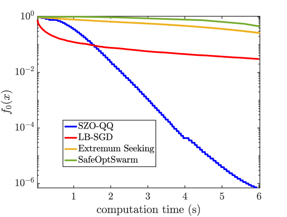
Figure 1: Objective value as a function of computation time.

In Fig. 1, we show the objective function values versus the computation time. During the experiments, none of the methods violates the constraints. Regarding the convergence to the minimum, we see that LB-SGD has the most decrease in the objective function value in the first 1.5 seconds due to the low complexity of each iteration. In these 1.5 seconds, LB-SGD utilizes 67856 function samples while SZO-QQ only 252. Afterward, SZO-QQ achieves a better solution. In the first 6 seconds, SZO-QQ shows a clear convergence trend to the optimum, consistent with Theorem 2, while SafeOptSwarm only finishes 6 iterations and 28 function samples.

LB-SGD slows down when the iterates are close to the boundary of the feasible set (see Appendix B for the explanation for this phenomenon). Meanwhile, the slow convergence of Extremum Seeking is due to its small learning rate. If the learning rate is large, the iterates might be brought too close to the boundary of the feasible set, and then the perturbation added by this method would lead to constraint violation. These considerations constitute the main dilemma in parameter tuning for Extremum Seeking. Meanwhile, exploring the unknown functions in SafeOptSwarm is based on Gaussian Process (GP) regression models instead of local perturbations. Since SafeOptSwarm does not exploit the convexity of the problem, it maintains a safe set and tries to expand it to find the global minimum. Empirically, this method samples many points close to the boundary of the feasible region, which is also observed in [18]. These samples along with the computational complexity of GP regression, are the main reason for the slow convergence of SafeOptSwarm. We also run LB-SGD and Extremum Seeking with different penalty coefficients $\mu_{\mathrm{log}}$ to check whether the slow convergence is due to improper parameter tuning. We see that with larger $\mu_{\mathrm{log}}$ the performance of the log-barrier-based methods deteriorates. This is probably because the optimum of the unconstrained problem $f_{\log}(x,\mu_{\log})$ deviates more from the optimum as $\mu_{\mathrm{log}}$ increases. With smaller $\mu_{\mathrm{log}}$, the Extremum Seeking method leads to constraint violation while the performance of LB-SGD barely changes.

6.1.3 Impact of the parameters $L_{i}$ and $M_{i}$

To show the impact of conservative guesses of $L_{i}$ and $M_{i}$, we consider 9 test cases of different values for the pair $(L,M)$. We use $L$ as the Lipschitz constant for all the objective and constraint functions and $M$ as the smoothness constant. We illustrate in Figures 2 and 3 the decrease of the objective function values when SZO-QQ and LB-SGD are applied to solve the 9 test cases. From the figures, we see that the time required by SZO-QQ to achieve an objective function value less than $10^{-2}$ grows with $M$. Despite this, across all the cases SZO-QQ is the first to achieve an objective function value of $10^{-2}$. Another observation is that the performance of SZO-QQ is more sensitive to varying $M$ while LB-SGD is more sensitive to varying $L$. This is due to the differences in the local feasible set formulations in both methods. Indeed, in SZO-QQ the constant $L_{i}$ is only related to the gradient estimation, and the size of the local feasible set $\mathcal{S}^{(k)}(\cdot)$ in (8) is mainly decided by $M_{i}$, while in LB-SGD the size of $\mathcal{T}^{(k)}(\cdot)$, for any $k$, is mainly dependent on the Lipschitz constants $L_{i}$ for $i\geq 1$.

We also study the case where the initial guesses of Lipschitz and smoothness constants are wrong, i.e., (3) in Assumption 1 is violated. With $L=0.2$ and $M=0.2$, we encounter an infeasible sample. Then we follow the method in Remark 3 to multiply the constants by 2 every time an infeasible sample is generated. With $L=M=0.8$, every sample is feasible and we derive in 2 seconds an objective function value of $4\times 10^{-7}$. In total, we generate two infeasible samples. Although the setting $L=M=0.8$ still fails to satisfy Assumption 1, with these constants, SZO-QQ is able to generate iterates that have a subsequence converging to a KKT pair. The readers can check that Theorem 2 holds even if the guesses for Lipschitz and smoothness constants do not verify (3) in Assumption 1 (see the proof of Theorem 2 in Appendix E).

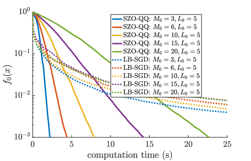
Figure 2: Objective value as a function of computation time:
$\;L_{0}=3$ fixed and $M_{0}$ varied

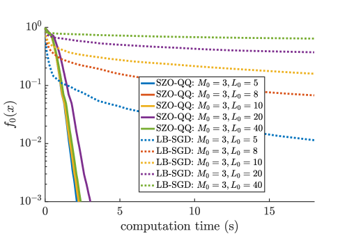
Figure 3: Objective value as a function of computation time:
$\;M_{0}=3$ fixed and $L_{0}$ varied

6.2 Open-loop optimal control with unmodelled disturbance

SZO-QQ can be applied to deterministic optimal control problems with unknown nonlinear dynamics by using only feasible samples. To illustrate, we consider a nonlinear system with dynamics $x_{k+1}=Ax_{k}+Bu_{k}+\delta(x_{k})[1\;0]^{\top}$, where $x_{k}\in\mathbb{R}^{2}$ for $k\geq 0$ and $x_{0}=[1\;1]^{\top}$. The matrices

$$A=\begin{bmatrix}1.1&1\\ -0.5&1.1\end{bmatrix},B=\begin{bmatrix}1&0\\ 0&1\end{bmatrix}$$

and the expression of the disturbance $\delta(x):=0.1*(x^{(2)})^{2}$ are unknown. We aim to design the input $u_{k}$ for $i\in\mathbb{Z}^{5}_{0}$ to minimize the cost $\sum^{5}_{k=0}\left(x_{k+1}^{\top}Qx_{k+1}+u_{k}^{\top}Ru_{k}\right)$ where $Q=0.5\,\mathbf{I}_{2}$ and $R=2\,\mathbf{I}_{2}$ with identity matrix $\mathbf{I}_{2}\in\mathbb{R}^{2\times 2}$ while enforcing $\|x_{k+1}\|_{\infty}\leq 0.7$ and $\|u_{k}\|_{\infty}\leq 1.5$ for $0\leq k\leq 5$. Since we assume all the states are measured, we can evaluate the objective and constraints. In this example, we assume to have a feasible sequence of inputs $\{u_{k}\}_{0\leq k\leq 5}$ that leads to a safe trajectory and results in a cost of 6.81 (as in Assumption 2). Different from the settings in the model-based safe learning control methods [55, 8], we do not assume that this safe trajectory is sufficient for identifying the system dynamics with small error bounds. If the error bounds are huge, the robust control problems formulated in [55, 8] may become infeasible.

We run SZO-QQ to further decrease the cost resulting from the initial safe trajectory and derive within 146 seconds of computation an input sequence that satisfies all the constraints and achieves a cost of 5.96. This cost is the same as the one obtained when assuming the dynamics are known and applying the solver IPOPT [56]. This observation is consistent with Theorem 2 on the convergence to a KKT pair. In this experiment, we set $L_{i}=M_{i}=20$ for $i\geq 1$, $\mu=10^{-4}$ and $\eta=10^{-1}$. Thus, the parameter $\xi$ adopted is $2\times 10^{-5}$ according to (13).

6.3 Optimal power flow for an unmodelled electric network

In this section, we apply SZO-QQ to solve the AC Optimal Power Flow (OPF) for the IEEE 30-bus system, described in [57]. In real-world power systems, it is often hard to obtain an accurate model of a power grid due to unmodelled disturbances (including aging of the devices and external attacks [58]). In [22], extremum seeking is used to solve OPF in a model-free way. As discussed in Section 6.1, using perturbation signals makes it difficult to select the barrier function coefficient. In this experiment, we aim to compare the results provided by SZO-QQ, which is model-free, with those produced by an OPF solver that utilizes the perfect model.

In the IEEE 30-bus system, the loads in the network are assumed to be fixed. Six generators are installed, among which one is the slack bus. The slack bus is assumed to provide the active power that is needed to maintain the AC frequency. The 11 decision variables are the voltage magnitude of the 6 generator nodes and the active power generations of the generators, except the slack bus. The cost is a quadratic function of the power generations, and 142 constraints are posed such that the power transmitted through any line is less than the rated value and the voltage magnitude of any bus is within the safe range.

We do not assume to know the system model for the optimization tasks. However, given a set of values for all the 11 decision variables, we can utilize a black-box simulation model in Matpower [59] to sample the voltages of all the 30 buses and the power through all the transmission lines in this network. We also assume to have initial values for all the decision variables such that the constraints are satisfied. In practice, initial values of the decision variables verifying the safety constraints in power systems are not hard to find due to various mechanisms for robust operation, e.g., droop control for power generation, shunt capacitor control and load shedding.

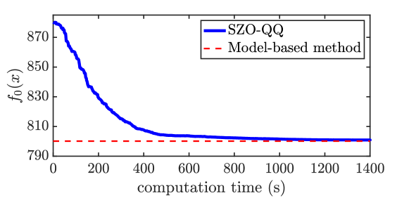
Figure 4: Objective value as a function of computation time

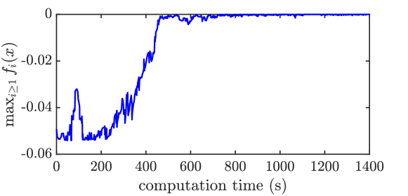
Figure 5: Largest constraint value as a function of computation time

In this experiment, we set $\mu=0.001$, $\xi=0.002$, $\Lambda=2$, $M_{i}=0.2$ and $L_{i}=1$ for $i\geq 1$. In Figure 4, we illustrate the decrease of the cost and compare it with the cost derived by using Gurobi [60] to solve the model-based optimal power flow. We see that the achieved cost within 1400 seconds is close to what the model-based method derives, which is again consistent with Theorem 2. Meanwhile, from Figure 5, which depicts the largest constraint function value with respect to the computation time, we see that, even though the decision variables can get very close to the boundary of the feasible set, the constraints are never violated.

Compared with only 1 second used by the model-based method to derive the solution, SZO-QQ is slow. One reason is that solving the QCQP subproblems of SZO-QQ takes too much time for this experiment. Our future work is to see whether the subproblems can be modified to be quadratic programs or even linear programs, which allow for more efficient solvers.

7 Conclusions

For safe black-box optimization problems, we proposed a method, SZO-QQ, based on samples of the objective and constraint functions to iteratively optimize over local feasible sets. Each iteration of our algorithm involves a QCQP subproblem, which can be solved efficiently. We showed that a subsequence of the algorithm’s iterates converges to a KKT pair and no infeasible samples are generated. Given any $\eta>0$, we proposed termination conditions dependent on $\eta$ such that the values returned by the algorithm form an $\eta$-KKT pair. The number of samples required is shown to be $O(\frac{1}{\eta^{2}})$ under mild assumptions. In comparison, the state-of-the-art methods LB-SGD and SafeOPT require $O(\frac{1}{\eta^{3}})$ and $O(\frac{1}{\eta^{2}})$ samples respectively. From numerical experiments, we see that our method can be faster than existing zeroth-order approaches, including LB-SGD, SafeOptSwarm, and Extremum Seeking. Furthermore, the results derived by SZO-QQ are very close to those generated by model-based methods. Future research directions include deriving a tighter complexity bound and generalizing the method for guaranteeing safety even when the samples are noisy.

Appendix

Appendix A Proof of Theorem 1

We notice that $\nu_{0}^{*}\leq l_{0}^{*}$ and, from Assumption 1, $f_{i}(x_{0}+\nu_{0}^{*}e_{j})<f_{i}(x_{0})+l_{0}^{*}L_{\max}=0$ for any $i\in\mathbb{Z}_{1}^{m},\,j\in\mathbb{Z}_{1}^{d}$. which shows the samples’ feasibility. To show the feasibility of $\mathcal{S}^{(0)}(x_{0})$, we first partition $\mathcal{S}^{(0)}_{i}(x_{0})$ as

$$\mathcal{S}^{(0)}_{i}(x_{0})=\left(\mathcal{S}^{(0)}_{i}(x_{0})\bigcap\mathcal{B}_{l^{*}_{0}}(x_{0})\right)\left.\left.\bigcup\right(\mathcal{S}^{(0)}_{i}(x_{0})\setminus\mathcal{B}_{l^{*}_{0}}(x_{0})\right)$$

and notice that $\mathcal{S}^{(0)}_{i}(x_{0})\bigcap\mathcal{B}_{l^{*}_{0}}(x_{0})\subseteq\Omega$. Then, it only remains to show $\mathcal{S}^{(0)}_{i}(x_{0})\setminus\mathcal{B}_{l^{*}_{0}}(x_{0})\subseteq\Omega.$

For $x\in\mathcal{S}^{(0)}_{i}(x_{0})\setminus B_{l^{*}_{0}}(x_{0})$, we have ${\sqrt{d}\nu^{*}_{0}}=l^{*}_{0}\leq\|x-x_{0}\|.$ By the mean value theorem, for any $i$ there exists $\theta_{i}\in[0,1]$ such that

$$f_{i}(x)= f_{i}(x_{0})+\nabla f_{i}\left(x_{0}+\theta_{i}(x-x_{0})\right)^{\top}(x-x_{0})$$ (14)

$$= f_{i}(x_{0})+\nabla f_{i}\left(x_{0}\right)^{\top}(x-x_{0})+$$

$$\left(\nabla f_{i}\left(x_{0}+\theta_{i}(x-x_{0})\right)-\nabla f_{i}\left(x_{0}\right)\right)^{\top}(x-x_{0})$$

$$\leq f_{i}(x_{0})+{\nabla}^{\nu^{*}_{0}}f_{i}\left(x_{0}\right)^{\top}(x-x_{0})$$

$$+\frac{\sqrt{d}\nu^{*}_{0}M_{i}}{2}\|x-x_{0}\|+M_{i}\|x-x_{0}\|^{2}$$

$$\leq f_{i}(x_{0})+{\nabla}^{\nu^{*}_{0}}f_{i}\left(x_{0}\right)^{\top}(x-x_{0})+2M_{i}\|x-x_{0}\|^{2}$$

$$\leq 0,$$

where the first inequality is due to Assumption 1 while the second one can be derived from the definition of $\nu^{*}_{0}$ in Theorem 1. Hence, $\mathcal{S}^{(0)}_{i}(x_{0})\setminus\mathcal{B}_{l^{*}_{0}}(x_{0})\subseteq\Omega.$ Since $\mathcal{S}^{(0)}_{i}(x_{0})\subseteq\Omega,\forall i$, then $\mathcal{S}^{(0)}(x_{0})\subseteq\Omega$. $\blacksquare$

Appendix B Comparison between two different formulations of local safe sets

The works  [61, 17] adopt an alternative approximation of the constraints and in particular form a local feasible set

$$\mathcal{T}^{(0)}(x_{0}):=\bigcap^{m}_{i=1}\left\{x:\|x-x_{0}\|\leq-\frac{f_{i}(x_{0})}{L_{i}}\right\}.$$

We see that $\mathcal{T}^{(0)}(x_{0})=\{x:F^{L}_{i}(x)\leq 0,\forall i\}$ where $F^{L}_{i}(x):=f_{i}(x_{0})+L_{i}\|x-x_{0}\|$ is linear in $\|x-x_{0}\|$. In contrast, $\mathcal{S}^{(0)}(x_{0})=\{x:F^{M}_{i}(x)\leq 0,\forall i\}$ where $F^{M}_{i}(x):=f_{i}(x_{0})+{\nabla}^{\nu^{*}_{0}}f_{i}\left(x_{0}\right)^{\top}(x-x_{0})+2{M}_{i}\|x-x_{0}\|^{2}$ is a quadratic approximation of $f_{i}(x)$. In the following proposition, we show that, if $x_{0}$ is sufficiently close to the boundary of the feasible set, $\mathcal{T}^{(0)}(x_{0})\subset\mathcal{S}^{(0)}(x_{0})$, which means that $\mathcal{S}^{(0)}(x_{0})$ is less conservative.

Proposition 3

Let ${\ell_{\min}}=\min_{i\geq 1}(L_{i}-L_{i,\mathrm{inf}})$. For $x_{0}$, if

$${\min_{i\geq 1}}-f_{i}(x_{0})\leq\frac{L_{\max}{\ell_{\min}}}{4{M_{\max}}},$$ (15)

then $\mathcal{T}^{(0)}(x_{0})\subset\mathcal{S}^{(0)}(x_{0})$.

Proof. For any $x\in\mathcal{T}^{(0)}(x_{0})$, we have

$$\|x-x_{0}\|\leq{\frac{\min-f_{i}(x_{0})}{L_{\max}}}\leq{\frac{{\ell_{\min}}}{4M_{\max}}}$$

and thus

$$2{M_{\max}}\|x-x_{0}\|^{2}\leq\frac{\ell_{\min}}{2}\|x-x_{0}\|.$$ (16)

Considering $\nu^{*}_{0}=\frac{\min-f_{i}(x_{0})}{\sqrt{d}{{L_{\max}}}}$ and (6), we have

$$\left\|\Delta^{\nu^{*}_{0}}_{i}(x)\right\|_{2}\leq\frac{\ell_{\min}}{2}$$

and thus

$$\nabla^{\nu^{*}_{0}}f_{i}(x_{0})^{\top}(x-x_{0})= (\nabla f_{i}(x_{0})+\Delta_{i}^{\nu^{*}_{0}}(x))^{\top}(x-x_{0})$$ (17)

$$\leq L_{i,\mathrm{inf}}\|x-x_{0}\|+\frac{\ell_{\min}}{2}\|x-x_{0}\|$$

By summing up (16) and (17), we have for any $x\in\mathcal{T}^{(0)}(x_{0})$

$$F^{M}_{i}(x)\leq f_{i}(x_{0})+{{L_{i}}}\|x-x_{0}\|=F^{L}_{i}(x)\leq 0,$$

and thus $x\in\mathcal{S}^{(0)}(x_{0})$. $\blacksquare$

Appendix C Proof of Theorem 1

Proof of Point 1. Given any $k$, we have $x_{k}\in\mathcal{S}^{(k)}(x_{k})$ and $x_{k+1}=\operatorname*{arg\,min}_{x\in\mathcal{S}^{(k)}(x_{k})}f_{0}(x)+\mu\|x-x_{k}\|^{2}$. Thus,

$$f_{0}(x_{k+1})+\mu\|x_{k+1}-x_{k}\|^{2}$$ (18)

$$\leq f_{0}(x_{k})+\mu\|x_{k}-x_{k}\|^{2}=f_{0}(x_{k}).$$

Proof of Point 2. For $k\geq 0$, one has $f_{0}(x_{k})\leq f_{0}(x_{0})<\beta$ according to Assumption 3. Now we know $\{x_{k}\}_{k\geq 1}$ is within the set $\mathcal{P}_{\beta}$. Due to the boundedness of the set $\mathcal{P}_{\beta}$, we can use Bolzano–Weierstrass theorem to conclude that there exists a subsequence of $\{x_{k}\}_{k\geq 1}$ that converges. Hence, $\{x_{k}\}_{k\geq 1}$ has at least one accumulation point $x_{c}$. According to (18), $f_{0}(x_{k+1})\leq f_{0}(x_{1})-\mu\sum_{i=1}^{k}\|x_{i+1}-x_{i}\|^{2}$. Since $f_{0}(x)$ is a continuous function on the compact set $\mathcal{P}_{\beta}$, $\mathrm{inf}_{x\in\mathcal{P}_{\beta}}f_{0}(x)>-\infty$. Therefore, $\sum_{i=1}^{\infty}\|x_{i+1}-x_{i}\|^{2}<\infty$ and $\|x_{k+1}-x_{k}\|$ converges to 0.

Proof of Point 3. The sequence $\{f_{0}(x_{k})\}_{k\geq 1}$ converging to $f_{0}(x_{c})$ is a direct consequence of Point 2 in Theorem 1 and the continuity of $f_{0}(x)$. $\blacksquare$

Appendix D Preliminary results towards the proof of Theorem 2

Lemma 4

If Assumption 4 holds, then

1. there exists $x\in\Omega$ that is strictly feasible with respect to $\mathcal{S}(x_{c})$, i.e. for any $i\geq 1$, $f^{c}_{i}(x)<0$ where

$$f^{c}_{i}(x):=f_{i}(x_{c})+\nabla f_{i}(x_{c})^{\top}(x-x_{c})+2M_{i}\|x-x_{c}\|^{2}.$$

For any $x\in\Omega$ verifying $f^{c}_{i}(x)<0$ for any $i$, there exists $k\in\mathbb{N}$ such that $x$ belongs to $\mathcal{S}^{(k)}(x_{k})$;

2. there exists $x_{s}\in\mathcal{S}(x_{c})$ such that $x_{s}\neq x_{c}$. For any such $x_{s}$ and any $0<t<1$, we let $x(t)=tx_{c}+(1-t)x_{s}$ and have that $x(t)$ is strictly feasible with respect to $\mathcal{S}(x_{c})$.

Proof of Point 1. We let $\mathcal{A}(x_{c})=\{i_{1},\ldots,i_{l}\}$. There exists $y\in\mathbb{R}^{d}$ such that

$$Jy=\begin{bmatrix}-1\\ \vdots\\ -1\end{bmatrix}\text{, where }J=\begin{bmatrix}\nabla f_{i_{1}}(x_{c})^{\top}\\ \vdots\\ \nabla f_{i_{l}}(x_{c})^{\top}\end{bmatrix},$$ (19)

because $J$ is full row rank due to LICQ. For any $y$ satisfying (19), if $\epsilon_{0}=1/(4M_{\max}\|y\|)$, then, for any $\epsilon<\epsilon_{0}$, $x=x_{c}+\epsilon y/\|y\|$ and $i\in\mathcal{A}(x_{c}),$

$$f^{c}_{i}(x)=0-\epsilon/\|y\|+2M_{i}\epsilon^{2}<0.$$

Since $f_{i}(x_{c})<0$ for any $i\notin\mathcal{A}(x_{c})$, there exists $\epsilon_{c}>0$ such that, for $\epsilon<\epsilon_{c}$ and $x=x_{c}+\epsilon_{c}y/\|y\|$, $f^{c}_{i}(x)<0$ for any $i\notin\mathcal{A}(x_{c})$. Thus, with $\epsilon=\min\{\epsilon_{0},\epsilon_{c}\}$ and $x=x_{c}+\epsilon y/\|y\|$, we have $f^{c}_{i}(x)<0$ for any $i$. Since $x_{c}$ is an accumulation point, there exists $k\in\mathbb{N}$ such that $x$ belongs to $\mathcal{S}^{(k)}(x_{k})$. $\hfill\blacksquare$

Proof of Point 2. We utilize the first point and the fact that $x_{c}$ is not strictly feasible with respect to $\mathcal{S}(x_{c})$ to conclude that there exists $x_{s}\in\mathcal{S}(x_{c})$ verifying $x_{s}\neq x_{c}$. Considering that $f^{c}_{i}(x)$ is strongly convex, we have, for any $i$ and any $0<t<1$, $f^{c}_{i}(x(t))<\max\{f^{c}_{i}(x_{c}),f^{c}_{i}(x_{s})\}\leq 0.$ $\hfill\blacksquare$

Before stating another preliminary result, we have the following notations based on the feasible region $\mathcal{S}^{(k)}(x_{k})$ of the subproblem (SP1) of Algorithm 1. We define for strictly feasible $x\in\Omega$,

$$O^{(k)}_{i}(x):= x-\frac{\nabla^{\nu^{*}_{k}}f_{i}(x)}{2M_{i}},$$ (20)

$$\left(r^{(k)}_{i}(x)\right)^{2}:= -\frac{f_{i}(x)}{M_{i}}+\frac{\|\nabla^{\nu^{*}_{k}}f_{i}(x)\|^{2}}{4M_{i}^{2}},$$

which allows us to write

$$\mathcal{S}^{(k)}_{i}(x_{k})=\mathcal{B}_{r^{(k)}_{i}(x_{k})}(O^{(k)}_{i}(x_{k})).$$

We let $\{x_{k_{p}}\}_{p\geq 1}$ be a subsequence converging to $x_{c}$. Since $\{\nu^{*}_{k}\}_{k\geq 1}$ converges to 0 (see (9)), we have

$$O^{(k_{p})}_{i}(x_{k_{p}})\rightarrow O_{i}(x_{c}),\text{ }r^{(k_{p})}_{i}(x_{k_{p}})\rightarrow r_{i}(x_{c})\text{ as }p\rightarrow\infty,$$ (21)

where

$$O_{i}(x_{c}):=x_{c}-\frac{\nabla f_{i}(x_{c})}{2M_{i}}\text{, }\left(r_{i}(x_{c})\right)^{2}:=-\frac{f_{i}(x)}{M_{i}}+\frac{\|\nabla f_{i}(x_{c})\|^{2}}{4M_{i}^{2}}.$$

Then, we write

$$\mathcal{S}_{i}(x_{c}):=\mathcal{B}_{r_{i}(x_{c})}(O_{i}(x_{c})),\mathcal{S}(x_{c}):=\bigcap^{m}_{i=1}\mathcal{S}_{i}(x_{c}).$$

With these notations, we can state and prove the following lemma.

Lemma 5

Under Assumption 4, the accumulation point $x_{c}$, where LICQ holds, is the unique optimum of the convex optimization

$$\min_{x\in\mathcal{S}(x_{c})}f_{0}(x)+\mu\|x-x_{c}\|^{2}.$$ (22)

Moreover, the optimizer $\lambda_{c}$ for the dual variable of (22) is also unique.

Proof. We prove the optimality of $x_{c}$ by contradiction. Assume $x_{c}$ is not the optimum of (22), then there exists $x_{s}\in\mathcal{S}(x_{c})$ verifying $f_{0}(x_{s})+\mu\|x_{s}-x_{c}\|^{2}<f_{0}(x_{c})$. According to the second point of Lemma 4 in Appendix D and the continuity of $f_{0}(x)$, there exists $0<t<1$ such that with $x(t)=tx_{c}+(1-t)x_{s}$ we have $f_{0}(x(t))+\mu\|x(t)-x_{c}\|^{2}<f_{0}(x_{c})$ and $x(t)$ is strictly feasible with respect to $\mathcal{S}(x_{c})$. We let $\{x_{k_{p}}\}_{p\geq 1}$ be a subsequence of $\{x_{k}\}_{k\geq 1}$ that converges to $x_{c}$. Considering the first point of Lemma 4, there exists $p$ such that $x(t)\in\mathcal{S}^{(k_{p})}(x_{k_{p}})$. Because of the convergence of the subsequence, we can assume without loss of generality that $p$ is sufficiently large so that $f_{0}(x(t))+\mu\|x(t)-x_{k_{p}}\|^{2}<f_{0}(x_{c})$. Due to the optimality of $x_{k_{p}+1}$ for the problem (SP1) in Algorithm 1 when $k=k_{p}$, we have $f_{0}(x_{k_{p}+1})+\mu\|x_{k_{p}+1}-x_{k_{p}}\|^{2}<f_{0}(x_{c})$, which contradicts the monotonicity of $\{f_{0}(x_{k})\}_{k\geq 1}$ in Theorem 1. Due to optimality of $x_{c}$ and LICQ, there exists $\lambda_{c}\in\mathbb{R}^{m}$ such that $(x_{c},\lambda_{c})$ is a KKT pair of (22).

We prove the uniqueness of $x_{c}$ and $\lambda_{c}$ also by contradiction. Assume there exists $x_{o}\in\mathcal{S}(x_{c})\setminus\{x_{c}\}$ such that $f_{0}(x_{o})+\mu\|x_{o}-x_{c}\|^{2}=f_{0}(x_{c})$. Due to the strong convexity of the function $f_{0}(x)+\mu\|x-x_{c}\|^{2}$, we know

$$f_{0}(\frac{x_{o}+x_{c}}{2})+\mu\|\frac{x_{o}+x_{c}}{2}-x_{c}\|^{2}<f_{0}(x_{c}),$$

which contradicts the optimality of $x_{c}$ for (22). Assume $(x_{c},\lambda_{c,1})$ and $(x_{c},\lambda_{c,2})$ are two KKT pairs of (22) with $\lambda_{c,1}\neq\lambda_{c,2}$, then for $j=1,2$, $\lambda_{c,j}^{(i)}=0$ for any $i\neq\mathcal{A}(x_{c})$,

$$\sum^{m}_{i=1}\lambda_{c,j}^{(i)}\nabla f_{i}(x_{c})=-\nabla f_{0}(x_{c})$$

and thus

$$\sum^{m}_{i=1}(\lambda_{c,1}^{(i)}-\lambda_{c,2}^{(i)})\nabla f_{i}(x_{c})=0.$$

This contradicts LICQ at $x_{c}$ since $\lambda_{c,1}-\lambda_{c,2}\neq 0.$ $\blacksquare$

Appendix E Proof of Theorem 2

According to Lemma 5, there exists a $\lambda_{c}\in\mathbb{R}^{m}$ such that $(x_{c},\lambda_{c})$ is a KKT pair of (22), i.e.,

$$\nabla f_{0}(x_{c})+\sum_{i\in\mathcal{A}(x_{c})}\lambda_{c}^{(i)}\nabla f_{i}(x_{c})=0$$

and $$\lambda_{c}^{(i)}=0\text{ for }i\notin\mathcal{A}(x_{c})\text{, }$$

which coincides with KKT conditions of (1). Thus, $(x_{c},\lambda_{c})$ is also a KKT pair of of (1). Following the same arguments used in the proof of Lemma 5, one can exploit LICQ to show that there does not exist $\lambda_{c,2}\neq\lambda_{c}$ such that $(x_{c},\lambda_{c,2})$ is a KKT pair of (1). $\blacksquare$

Appendix F Geometric illustration of an upperbound to $\|\lambda_{c}\|_{\infty}$

We consider an instance of the optimization problem (1) where $d=2$, the feasible region is convex, and $(x_{c},\lambda_{c})$ is a KKT pair. We only consider the non-degenerate case where $\mathcal{A}(x_{c})=\{1,2\}$ and assume LICQ holds at $x_{c}$, i.e., $\nabla f_{i}(x_{c})$ are linearly independent for $i=1,2.$ The objective and constraint functions are normalized at $x_{c}$, i.e., $\|\nabla f_{i}(x_{c})\|=1$ for $i\in\mathbb{Z}^{2}_{0}.$ Then, we use coordinate transformation such that $\nabla f_{0}(x_{c})=\begin{bmatrix}0&-1\end{bmatrix}^{\top}.$ Since $\mathcal{A}(x_{c})=\{1,2\}$, the KKT pair $(x_{c},\lambda_{c})$ satisfies that $\lambda_{c}^{(1)},\lambda_{c}^{(2)}\geq 0$ and

$$f_{1}(x_{c})\leq 0,\text{ }f_{2}(x_{c}) \leq 0$$ (23)

$$\nabla f_{0}(x_{c})+\lambda^{(1)}_{c}\nabla f_{1}(x_{c})+\lambda^{(2)}_{c}\nabla f_{2}(x_{c}) =0$$

$$\lambda^{(1)}_{c}f_{1}(x_{c})=0,\text{ }\lambda^{(2)}_{c}f_{2}(x_{c}) =0.$$

Let $\theta_{i}$ be the angle between $-\nabla f_{0}(x_{c})$ and $\nabla f_{i}(x_{c})$ for $i=1,2.$ Due to the convexity of the feasible region, $0<\theta_{1}+\theta_{2}<\pi.$ By solving (23), we have that

$$\lambda^{(1)}_{c}=\frac{|\sin\theta_{2}|}{\sin(\theta_{1}+\theta_{2})},\;\lambda^{(2)}_{c}=\frac{|\sin\theta_{1}|}{\sin(\theta_{1}+\theta_{2})}.$$

We illustrate in Fig. 6 how to construct $\theta_{1}$ and $\theta_{2}$.

We notice that

$$\|\lambda_{c}\|_{\infty}<(\sin\theta)^{-1},$$

where $\theta=\pi-\theta_{1}-\theta_{2}$ is the angle between the two lines $l_{1}:=\{x:(x-x_{c})^{\top}\nabla f_{1}(x_{c})=0\}$ and $l_{2}:=\{x:(x-x_{c})^{\top}\nabla f_{2}(x_{c})=0\}$. These two lines are actually the boundaries formed by the constraint functions $f_{1}(x)$ and $f_{2}(x)$ linearized at $x=x_{c}$. From the above conclusions, we see that for 2-dimensional optimization problems we need a large $\Lambda$ to satisfy Assumption 5 only when the angle $\theta$ is small.

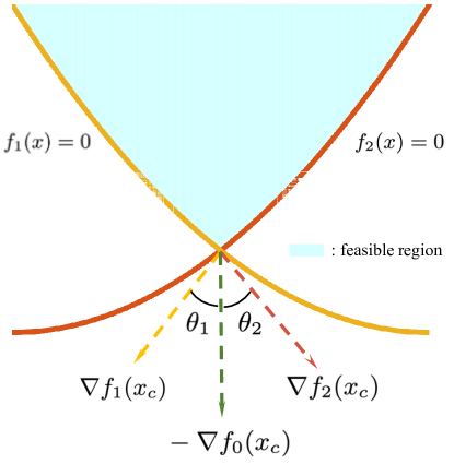
Figure 6: The illustration of angles $\theta_{1}$ and $\theta_{2}$

Appendix G Proof of Lemma 2

We assume $x_{\tau}$ is an accumulation point of $\{x_{k}\}_{k\geq 1}$ and is also a strict local minimizer. We show the convergence of $\{x_{k}\}_{k\geq 1}$ by contradiction and assume that $\mathcal{C}\setminus\{x_{\tau}\}\neq\emptyset$, where $\mathcal{C}$ is the set of accumulation points of $\{x_{k}\}_{k\geq 1}$. Then, there exists $\epsilon>0$ such that $\mathcal{C}\cap(\Omega\setminus\mathcal{B}_{\epsilon}(x_{\tau}))\neq\emptyset$ and any $x\in\mathcal{B}_{\epsilon}(x_{\tau})\setminus\{x_{\tau}\}$ verifies $f_{0}(x_{\tau})<f_{0}(x)$. Since the sphere $\mathcal{SP}_{\epsilon}(x_{\tau})=\{x:\|x-x_{\tau}\|=\epsilon\}$ is compact, we let $\sigma=\inf_{x\in\mathcal{SP}_{\epsilon}(x_{\tau})}f_{0}(x)$ and have $\sigma>f_{0}(x_{\tau})$. Therefore, there exists $k_{\alpha}>0$ such that $f_{0}(x_{k_{\alpha}})<(\sigma+f_{0}(x_{\tau}))/2$.

Since there exists an accumulation point outside $\mathcal{B}_{\epsilon}(x_{\tau})$ and $\{x_{k+1}-x_{k}\}_{k\geq 1}$ converges to 0, we can find $k_{\beta}>k_{\alpha}$ such that $x_{k_{\beta}}\in\mathcal{B}_{\epsilon}(x_{\tau})$, $x_{k_{\beta}+1}\notin\mathcal{B}_{\epsilon}(x_{\tau})$ and $\|x_{k_{\beta}+1}-x_{k_{\beta}}\|\leq(\sigma-f_{0}(x_{\tau}))/(4L_{\max})$. Let $\tilde{x}=\{x:\text{there exists }t\in[0,1]\text{ such that ${x}=tx_{k_{\beta}}+(1-t)x_{k_{\beta}+1}$}\}\cap\mathcal{SP}_{\epsilon}(x_{\tau})$, i.e., $\tilde{x}$ is the intersection of $\mathcal{SP}_{\epsilon}(x_{\tau})$ and the line segment between $x_{k_{\beta}}$ and $x_{k_{\beta}+1}$. Then, $\|x_{k_{\beta}}-\tilde{x}\|\leq(\sigma-f_{0}(x_{\tau}))/(4L_{\max})$ and thus

$$f_{0}(x_{k_{\beta}}) \geq f_{0}(\tilde{x})-\frac{\sigma-f_{0}(x_{\tau})}{4}$$

$$\geq\sigma-\frac{\sigma-f_{0}(x_{\tau})}{4}$$

$$>(\sigma+f_{0}(x_{\tau}))/2>f_{0}(x_{k_{\alpha}}),$$

which contradicts with the monotonicity of $\{f_{0}(x_{k})\}_{k\geq 1}$ shown in Theorem 1. $\blacksquare$

Appendix H Proof of Theorem 2

Since $(x_{c},\lambda_{c})$ is a KKT pair where $\|\lambda_{c}\|_{\infty}<\Lambda$, by using triangular inequalities on the norm terms defining $\delta_{1}(k,\lambda_{c})$, we obtain

$$\delta_{1}(k,\lambda_{c})$$

$$\leq \|{\nabla}f_{0}(x_{c})+\sum^{m}_{i=1}\lambda_{c}^{(i)}{\nabla}f_{i}\left(x_{c}\right)\|+\|{\nabla}f_{0}(x_{k})-{\nabla}f_{0}(x_{c})\|$$

$$+4\mu\|x_{k+1}-x_{k}\|+\sum^{m}_{i=1}\Lambda\Big{(}\|{\nabla}^{\nu_{k}^{*}}f_{i}\left(x_{k}\right)-{\nabla}f_{i}\left(x_{k}\right)\|$$

$$+\|{\nabla}f_{i}\left(x_{k}\right)-{\nabla}f_{i}\left(x_{c}\right)\|\Big{)}+4m{M_{\max}}\Lambda\|x_{k+1}-x_{k}\|.$$

Similar computations for $\delta^{(i)}_{2}(k,\lambda_{c})$ give

$$\delta^{(i)}_{2}(k,\lambda_{c})\leq |\lambda^{(i)}_{c}f_{i}(x_{c})|+\Lambda|f_{i}(x_{k})-f_{i}(x_{c})|$$

$$+\Lambda\Big{(}L_{i}|x_{k+1}-x_{k}|+2M_{i}\|x_{k+1}-x_{k}\|^{2}\Big{)}.$$

We let $\{x_{k_{p}}\}_{p\geq 1}$ be an subsequence that converges to $x_{c}$. Considering that the gradient estimation error converges to 0 (see (9) and Lemma 1), we know the term $\|{\nabla}^{\nu_{k_{p}}^{*}}f_{i}\left(x_{k_{p}}\right)-{\nabla}f_{i}\left(x_{k_{p}}\right)\|$ converges to 0 as $p$ goes to infinity. Therefore, we have

$$\lim_{p\rightarrow\infty}\delta_{1}(k_{p},\lambda_{c})=0\text{ and }\lim_{p\rightarrow\infty}\max_{1\leq i\leq m}|\delta^{(i)}_{2}(k_{p},\lambda_{c})|=0.$$

Thus, for any $k_{0}$ and $\eta>0$, one can find $k_{\Lambda}>k_{0}$ such that $\max\{\delta_{1}(k_{\Lambda},\lambda_{c}),\max_{1\leq i\leq m}|\delta^{(i)}_{2}(k_{\Lambda},\lambda_{c})|\}<\eta/2$. For $k=k_{\Lambda}$ in SZO-QQ, we have that $\lambda_{k_{\Lambda}+1}$, the solution to (SP2), has an infinite norm less than $2\Lambda$ because $\lambda_{c}$ is a feasible solution to (SP2) and $\|\lambda_{c}\|_{\infty}<2\Lambda$, which is to say that the second termination condition of Algorithm 1 is satisfied when $k=k_{\Lambda}$.

Since $\|x_{k+1}-x_{k}\|$ converges to 0 as $k$ goes to infinity (see Theorem 1), we can choose $k_{0}$ to be sufficiently large so that, for any $k>k_{0}$, $\|x_{k+1}-x_{k}\|\leq\xi$. Thus, when $k=k_{\Lambda}$, the two termination conditions are satisfied. $\blacksquare$

Appendix I Proof of Theorem 3

The pair $(\tilde{x},\tilde{\lambda})$ and the index $\tilde{k}$ returned by Algorithm 1 satisfy $\tilde{x}=x_{\tilde{k}}$ and

$$\max\Big{\{}\delta_{1}(\tilde{k},\tilde{\lambda}),\max\{\delta^{(i)}_{2}(\tilde{k},\tilde{\lambda}):i\geq 1\}\Big{\}}\leq\frac{\eta}{2}.$$ (24)

By using triangular inequalities we have for any $i$,

$$\|{\nabla}^{\nu_{\tilde{k}-1}^{*}}f_{i}\left(x_{\tilde{k}-1}\right)-{\nabla}f_{i}\left(x_{\tilde{k}}\right)\|$$

$$\leq \|{\nabla}^{\nu_{\tilde{k}-1}^{*}}f_{i}\left(x_{\tilde{k}-1}\right)-{\nabla}f_{i}\left(x_{\tilde{k}-1}\right)\|$$

$$\qquad\qquad\qquad\qquad+\|{\nabla}f_{i}\left(x_{\tilde{k}}\right)-{\nabla}f_{i}\left(x_{\tilde{k}-1}\right)\|$$

$$\leq \alpha\xi+L_{i}\xi.$$ (25)

Then, based on (13), (24) and (25), we have

$$||\nabla f_{0}\left(x_{\tilde{k}}\right)+\sum^{m}_{i=1}\tilde{\lambda}^{(i)}{\nabla}f_{i}\left(x_{\tilde{k}}\right)\|$$

$$\leq \Big{\|}\nabla f_{0}\left(x_{\tilde{k}}\right)+\sum^{m}_{i=1}\tilde{\lambda}^{(i)}\left({\nabla}^{\nu_{\tilde{k}-1}^{*}}f_{i}\left(x_{\tilde{k}-1}\right)+4M_{i}(x_{\tilde{k}}-x_{\tilde{k}-1})\right)$$

$$+2\mu(x_{\tilde{k}}-x_{\tilde{k}-1})\Big{\|}+\|2\mu(x_{\tilde{k}}-x_{\tilde{k}-1})\|$$

$$+2\Lambda\sum^{m}_{i=1}\Big{(}4\left\|M_{i}(x_{\tilde{k}}-x_{\tilde{k}-1})\right\|+\left\|{\nabla}^{\nu_{\tilde{k}-1}^{*}}f_{i}\left(x_{\tilde{k}-1}\right)-{\nabla}f_{i}\left(x_{\tilde{k}}\right)\right\|\Big{)}$$

$$\leq \eta/2+2\Lambda\sum^{m}_{i=1}\left(5M_{i}\xi+\alpha_{i}\nu^{*}_{\tilde{k}-1}\right)+2\mu\xi\leq\eta,$$

and

$$\left\|\tilde{\lambda}^{(i)}f_{i}(x_{\tilde{k}})\right\|$$

$$\leq \Big{\|}\tilde{\lambda}^{(i)}\Big{(}f_{i}(x_{\tilde{k}-1})+{\nabla}^{\nu_{\tilde{k}-1}^{*}}f_{i}\left(x_{\tilde{k}-1}\right)(x_{\tilde{k}}-x_{\tilde{k}-1})$$

$$+2M_{i}\|x_{\tilde{k}}-x_{\tilde{k}-1}\|^{2}\Big{)}\Big{\|}+2\Lambda\Big{(}\|f_{i}(x_{\tilde{k}})-f_{i}(x_{\tilde{k}-1})\|+$$

$$\|{\nabla}^{\nu_{\tilde{k}-1}^{*}}f_{i}\left(x_{\tilde{k}-1}\right)-{\nabla}f_{i}\left(x_{\tilde{k}-1}\right)\|\cdot\|x_{\tilde{k}}-x_{\tilde{k}-1}\|+$$

$$\|\nabla f_{i}(x_{\tilde{k}-1})\|\cdot\|x_{\tilde{k}}-x_{\tilde{k}-1}\|+2M_{i}\|x_{\tilde{k}}-x_{\tilde{k}-1}\|^{2}\Big{)}$$

$$\leq \eta/2+2\Lambda(2L_{i}\xi+\alpha_{i}\xi^{2}+2M_{i}\xi^{2})$$

$$\leq \eta/2+2\Lambda(2L_{i}+\alpha_{i}+2M_{i})\xi\leq\eta,$$

which concludes the proof. $\blacksquare$

Appendix J Proof of Lemma 3

We start by charaterizing $\mathcal{D}_{\lambda}(y,\nu)$. Since any $\lambda\in\mathcal{D}_{\lambda}(y,\nu)$ is an optimal solution to the dual variable, we have that

$$\mathcal{D}_{\lambda} (y,\nu):=$$

$$\operatorname*{arg\,max}_{\lambda\geq 0}\min_{x}f_{0}(x)+\mu\|x-y\|^{2}+\sum_{i=1}^{m}\lambda^{(i)}\Big{(}f_{i}(y)$$

$$\quad+\Big{(}\Delta^{\nu}_{i}(y)+\nabla f_{i}(y)\Big{)}^{\top}(x-y)+2M_{i}\|x-y\|^{2}\Big{)}.$$

By computing the inner minimization problem which is an unconstrained convex quadratic programming, we know that there exist $p\in\mathbb{R}^{m\times 1}_{\geq 0}$ and $a\in\mathbb{R}_{>0}$, independent of $y$ and $\nu$, such that

$$\mathcal{D}_{\lambda}(y,\nu)=\operatorname*{arg\,max}_{\lambda\geq 0}G(\lambda,y,\nu),$$

where for $\lambda\in\mathbb{R}^{m}_{\geq 0}$,

$$G(\lambda,y,\nu):=\frac{\lambda^{\top}Q(y,\nu)\lambda+q^{\top}(y,\nu)\lambda+b(y,\nu)}{p^{\top}\lambda+a},$$

the functions $Q(y,\nu)\in\mathbb{R}^{m\times m},q(y,\nu)\in\mathbb{R}^{m\times 1},b(y,\nu)\in\mathbb{R}$ are continuous in $(y,\nu)$ and $Q(y,\nu)$ is negative definite.

From the continuity of $Q(y,\nu),q(y,\nu)$ and $b(y,\nu)$, the function $G(\lambda,y,\nu)$ is continuous in all arguments for $\lambda\geq 0$. Due to the continuity and the uniqueness of the optimal dual solution $\mathcal{D}_{\lambda}(x_{c},0)=\{\lambda_{c}\}$ (see Lemma 5), we can use perturbation theory [62, Proposition 4.4] to conclude that $\mathcal{D}_{\lambda}(y,\nu)$ is upper semicontinuous at $(y,\nu)=(x_{c},0)$. Considering the definition of upper semicontinuity and the convergence of $(x_{k},\nu^{*}_{k})$ to $(x_{c},0)$, for any $\delta>0$, there exists $k_{\delta}>0$ such that $\mathcal{D}_{\lambda}(x_{k},\nu^{*}_{k})\subset\mathcal{B}_{\delta}(\lambda_{c})$ for any $k>k_{\delta}$. Since $\lambda^{\circ}_{k+1}\in\mathcal{D}_{\lambda}(x_{k},\nu^{*}_{k})\subset\mathcal{B}_{\delta}(\lambda_{c})$, we have $\lambda^{\circ}_{k+1}\in\mathcal{B}_{\delta}(\lambda_{c})$ for any $k>k_{\delta}$. $\blacksquare$

Appendix K Proof of Theorem 4

According to Lemma 3, there exists $\bar{k}>0$ such that $\|\lambda^{\circ}_{k+1}\|_{\infty}\leq 2\Lambda$ for any $k\geq\bar{k}$. Since $\lambda^{\circ}_{k+1}$ is a feasible solution of (SP2) in Algorithm 1, $\lambda_{k+1}$, the optimal solution of (SP2), also satisfies $\|\lambda_{k+1}\|_{\infty}\leq 2\Lambda$.

We let $\bar{\xi}:=\inf_{k\leq\bar{k}}\|x_{k+1}-x_{k}\|$, $\bar{\eta}:=\inf\{\eta:h(\eta)\geq\bar{\xi}/2\}$ and consider the case where $\eta<\bar{\eta}$. We first notice that if $\|x_{k+1}-x_{k}\|\leq h(\eta)$, we have $\|x_{k+1}-x_{k}\|<\bar{\xi}$ and thus $k>\bar{k}$. We then let $\mathcal{K}(\eta):=\max\{k:\|x_{k+1}-x_{k}\|>h(\eta)\}+1$. Since $\|x_{\mathcal{K}(\eta)+1}-x_{\mathcal{K}(\eta)}\|\leq h(\eta)$, we have that $\mathcal{K}(\eta)>\bar{k}$ and thus $\|\lambda_{k+1}\|_{\infty}\leq 2\Lambda$, which is equivalent to say that with $k=\mathcal{K}(\eta)$, the two termination conditions in Algoirthm 1 are satisfied. Then $\tilde{k}$, the iteration number returned by Algorithm 1, verifies that $\tilde{k}\leq\mathcal{K}(\eta)+1$. According to (12),

$$f_{0}(x_{0})-\inf\{f_{0}(x):x\in\Omega\} \geq f_{0}(x_{0})-f_{0}(x_{\mathcal{K}(\eta)})$$ (26)

$$\geq\mu\mathcal{K}(\eta)(h(\eta))^{2}$$

and thus $\tilde{k}\leq\mathcal{K}(\eta)+1\leq\overline{\mathcal{K}}(\eta)+1$. Therefore, according to the definition of $h(\eta)$ in (13) there exists $A_{1}>0$ such that $\mathcal{K}(\eta)+1\leq A_{1}((L_{\max}+M_{\max})/\eta)^{2}$.

For $\eta\geq\bar{\eta}$, we let $A_{2}=\sup_{\eta\geq\bar{\eta}}\frac{(\mathcal{K}(\eta)+1)(L_{\max}+M_{\max})^{2}}{\eta^{2}}$. According to the definition of $\mathcal{K}(\eta)$, we have that $\mathcal{K}(\eta)$ is monotonously decreasing with respect to $\eta$. Therefore, $\mathcal{K}(\eta)\leq\mathcal{K}(\bar{\eta})\leq\overline{\mathcal{K}}(\bar{\eta})$ and thus $A_{2}$ is finite. Since $\mathcal{K}(\eta)+1\leq A_{2}((L_{\max}+M_{\max})/\eta)^{2}$, by letting $A=\max\{A_{1},A_{2}\}$, we have for any $\eta>0$, $\mathcal{K}(\eta)+1\leq A((L_{\max}+M_{\max})/\eta)^{2}.$ $\blacksquare$

References

- [1] Z. Chu, N. Zhang, and F. Teng, “Frequency-constrained resilient scheduling of microgrid: a distributionally robust approach,” IEEE Transactions on Smart Grid, vol. 12, no. 6, pp. 4914–4925, 2021.
- [2] Y. Chen, A. Orvieto, and A. Lucchi, “An accelerated DFO algorithm for finite-sum convex functions,” in Proceedings of the 37th International Conference on Machine Learning, ser. Proceedings of Machine Learning Research, vol. 119, 13–18 Jul 2020, pp. 1681–1690.
- [3] Z. Manchester and S. Kuindersma, “Derivative-free trajectory optimization with unscented dynamic programming,” in 2016 IEEE 55th Conference on Decision and Control (CDC). IEEE, 2016, pp. 3642–3647.
- [4] C. V. Rao, S. J. Wright, and J. B. Rawlings, “Application of interior-point methods to model predictive control,” Journal of optimization theory and applications, vol. 99, no. 3, pp. 723–757, 1998.
- [5] W. Xu, C. N. Jones, B. Svetozarevic, C. R. Laughman, and A. Chakrabarty, “Vabo: Violation-aware bayesian optimization for closed-loop control performance optimization with unmodeled constraints,” in 2022 American Control Conference (ACC). IEEE, 2022, pp. 5288–5293.
- [6] I. Bajaj, A. Arora, and M. Hasan, Black-Box Optimization: Methods and Applications. Springer, 2021, pp. 35–65.
- [7] M. Yousefi, K. van Heusden, I. M. Mitchell, J. M. Ansermino, and G. A. Dumont, “A formally-verified safety system for closed-loop anesthesia,” IFAC-PapersOnLine, vol. 50, no. 1, pp. 4424–4429, 2017.
- [8] L. Hewing, J. Kabzan, and M. N. Zeilinger, “Cautious model predictive control using gaussian process regression,” IEEE Transactions on Control Systems Technology, vol. 28, no. 6, pp. 2736–2743, 2019.
- [9] J. Nocedal and S. J. Wright, Numerical optimization. Spinger, 2006.
- [10] R. M. Lewis and V. Torczon, “Pattern search methods for linearly constrained minimization,” SIAM Journal on Optimization, vol. 10, no. 3, pp. 917–941, 2000.
- [11] S. Ghadimi and G. Lan, “Stochastic first-and zeroth-order methods for nonconvex stochastic programming,” SIAM Journal on Optimization, vol. 23, no. 4, pp. 2341–2368, 2013.
- [12] A. R. Conn, N. I. Gould, and P. L. Toint, Trust region methods. SIAM, 2000.
- [13] R. M. Lewis and V. Torczon, “A globally convergent augmented lagrangian pattern search algorithm for optimization with general constraints and simple bounds,” SIAM Journal on Optimization, vol. 12, no. 4, pp. 1075–1089, 2002.
- [14] I. Usmanova, A. Krause, and M. Kamgarpour, “Safe convex learning under uncertain constraints,” in The 22nd International Conference on Artificial Intelligence and Statistics. PMLR, 2019, pp. 2106–2114.
- [15] N. Echebest, M. L. Schuverdt, and R. P. Vignau, “An inexact restoration derivative-free filter method for nonlinear programming,” Computational and Applied Mathematics, vol. 36, no. 1, pp. 693–718, 2017.
- [16] I. Bajaj, S. S. Iyer, and M. F. Hasan, “A trust region-based two phase algorithm for constrained black-box and grey-box optimization with infeasible initial point,” Computers & Chemical Engineering, vol. 116, pp. 306–321, 2018.
- [17] Y. Sui, A. Gotovos, J. Burdick, and A. Krause, “Safe exploration for optimization with gaussian processes,” in International Conference on Machine Learning. PMLR, 2015, pp. 997–1005.
- [18] M. Turchetta, F. Berkenkamp, and A. Krause, “Safe exploration for interactive machine learning,” Advances in Neural Information Processing Systems, vol. 32, p. 2887–2897, 2019.
- [19] L. Sabug Jr, F. Ruiz, and L. Fagiano, “Smgo-: Balancing caution and reward in global optimization with black-box constraints,” Information Sciences, vol. 605, pp. 15–42, 2022.
- [20] A. P. Vinod, A. Israel, and U. Topcu, “Constrained, global optimization of unknown functions with lipschitz continuous gradients,” SIAM Journal on Optimization, vol. 32, no. 2, pp. 1239–1264, 2022.
- [21] C. Audet and J. E. Dennis Jr, “A progressive barrier for derivative-free nonlinear programming,” SIAM Journal on optimization, vol. 20, no. 1, pp. 445–472, 2009.
- [22] D. B. Arnold, M. Negrete-Pincetic, M. D. Sankur, D. M. Auslander, and D. S. Callaway, “Model-free optimal control of var resources in distribution systems: An extremum seeking approach,” IEEE Transactions on Power Systems, vol. 31, no. 5, pp. 3583–3593, 2015.
- [23] I. Usmanova, Y. As, M. Kamgarpour, and A. Krause, “Log barriers for safe black-box optimization with application to safe reinforcement learning,” arXiv preprint arXiv:2207.10415, 2022.
- [24] J. C. Willems, P. Rapisarda, I. Markovsky, and B. L. De Moor, “A note on persistency of excitation,” Systems & Control Letters, vol. 54, no. 4, pp. 325–329, 2005.
- [25] J. Coulson, J. Lygeros, and F. Dörfler, “Data-enabled predictive control: In the shallows of the deepc,” in 2019 18th European Control Conference (ECC). IEEE, 2019, pp. 307–312.
- [26] M. Yin, A. Iannelli, and R. S. Smith, “Maximum likelihood estimation in data-driven modeling and control,” IEEE Transactions on Automatic Control, 2021.
- [27] L. Furieri, B. Guo, A. Martin, and G. Ferrari-Trecate, “Near-optimal design of safe output feedback controllers from noisy data,” IEEE Transactions on Automatic Control, 2022.
- [28] J. F. Fisac, A. K. Akametalu, M. N. Zeilinger, S. Kaynama, J. Gillula, and C. J. Tomlin, “A general safety framework for learning-based control in uncertain robotic systems,” IEEE Transactions on Automatic Control, vol. 64, no. 7, pp. 2737–2752, 2018.
- [29] J. Achiam, D. Held, A. Tamar, and P. Abbeel, “Constrained policy optimization,” in International conference on machine learning. PMLR, 2017, pp. 22–31.
- [30] Z. Qin, D. Sun, and C. Fan, “Sablas: Learning safe control for black-box dynamical systems,” IEEE Robotics and Automation Letters, vol. 7, no. 2, pp. 1928–1935, 2022.
- [31] F. Berkenkamp, A. P. Schoellig, and A. Krause, “Safe controller optimization for quadrotors with gaussian processes,” in 2016 IEEE international conference on robotics and automation (ICRA). IEEE, 2016, pp. 491–496.
- [32] C. König, M. Turchetta, J. Lygeros, A. Rupenyan, and A. Krause, “Safe and efficient model-free adaptive control via bayesian optimization,” in 2021 IEEE International Conference on Robotics and Automation (ICRA). IEEE, 2021, pp. 9782–9788.
- [33] B. Guo, Y. Jiang, M. Kamgarpour, and G. F. Trecate, “Safe zeroth-order convex optimization using quadratic local approximations,” arXiv preprint arXiv:2211.02645, 2022.
- [34] S. Boyd and L. Vandenberghe, Convex optimization. Cambridge university press, 2004.
- [35] P. Jain, P. Kar et al., “Non-convex optimization for machine learning,” Foundations and Trends® in Machine Learning, vol. 10, no. 3-4, pp. 142–363, 2017.
- [36] J. B. Rawlings, D. Q. Mayne, and M. Diehl, Model predictive control: theory, computation, and design. Nob Hill Publishing Madison, WI, 2017, vol. 2.
- [37] P. S. Kundur and O. P. Malik, Power system stability and control. McGraw-Hill Education, 2022.
- [38] J. Dutta, K. Deb, R. Tulshyan, and R. Arora, “Approximate kkt points and a proximity measure for termination,” Journal of Global Optimization, vol. 56, no. 4, pp. 1463–1499, 2013.
- [39] G. N. Grapiglia and Y. Nesterov, “Tensor methods for finding approximate stationary points of convex functions,” Optimization Methods and Software, vol. 37, no. 2, pp. 605–638, 2022.
- [40] J.-P. Dussault, M. Haddou, A. Kadrani, and T. Migot, “On approximate stationary points of the regularized mathematical program with complementarity constraints,” Journal of Optimization Theory and Applications, vol. 186, no. 2, pp. 504–522, 2020.
- [41] A. Wibisono, M. J. Wainwright, M. Jordan, and J. C. Duchi, “Finite sample convergence rates of zero-order stochastic optimization methods,” Advances in Neural Information Processing Systems, vol. 25, 2012.
- [42] A. R. Conn, K. Scheinberg, and L. N. Vicente, Introduction to derivative-free optimization. SIAM, 2009.
- [43] A. Rupenyan, M. Khosravi, and J. Lygeros, “Performance-based trajectory optimization for path following control using bayesian optimization,” in 2021 60th IEEE Conference on Decision and Control (CDC). IEEE, 2021, pp. 2116–2121.
- [44] A. S. Berahas, L. Cao, K. Choromanski, and K. Scheinberg, “A theoretical and empirical comparison of gradient approximations in derivative-free optimization,” Foundations of Computational Mathematics, vol. 22, no. 2, pp. 507–560, 2022.
- [45] A. Y. Aravkin, R. Baraldi, and D. Orban, “A proximal quasi-newton trust-region method for nonsmooth regularized optimization,” SIAM Journal on Optimization, vol. 32, no. 2, pp. 900–929, 2022.
- [46] M. Fukushima, Z.-Q. Luo, and P. Tseng, “A sequential quadratically constrained quadratic programming method for differentiable convex minimization,” SIAM Journal on Optimization, vol. 13, no. 4, pp. 1098–1119, 2003.
- [47] F. Messerer and M. Diehl, “Determining the exact local convergence rate of sequential convex programming,” in 2020 European Control Conference (ECC). IEEE, 2020, pp. 1280–1285.
- [48] F. Messerer, K. Baumgärtner, and M. Diehl, “Survey of sequential convex programming and generalized gauss-newton methods,” ESAIM. Proceedings and Surveys, vol. 71, pp. 64–88, 2021.
- [49] G. Frison, J. Frey, F. Messerer, A. Zanelli, and M. Diehl, “Introducing the quadratically-constrained quadratic programming framework in hpipm,” in 2022 European Control Conference (ECC). IEEE, 2022, pp. 447–453.
- [50] G. Wachsmuth, “On LICQ and the uniqueness of lagrange multipliers,” Operations Research Letters, vol. 41, no. 1, pp. 78–80, 2013.
- [51] I. Usmanova, M. Kamgarpour, A. Krause, and K. Levy, “Fast projection onto convex smooth constraints,” in International Conference on Machine Learning. PMLR, 2021, pp. 10 476–10 486.
- [52] M. Zhu and E. Frazzoli, “Distributed robust adaptive equilibrium computation for generalized convex games,” Automatica, vol. 63, pp. 82–91, 2016.
- [53] M. Diehl, H. G. Bock, and J. P. Schlöder, “A real-time iteration scheme for nonlinear optimization in optimal feedback control,” SIAM Journal on control and optimization, vol. 43, no. 5, pp. 1714–1736, 2005.
- [54] A. F. Izmailov and M. V. Solodov, “Newton-type methods for optimization problems without constraint qualifications,” SIAM Journal on Optimization, vol. 15, no. 1, pp. 210–228, 2004.
- [55] D. D. Fan, A.-a. Agha-mohammadi, and E. A. Theodorou, “Deep learning tubes for tube mpc,” in Proceedings of Robotics: Science and Systems XVI, 2020.
- [56] A. Wächter and L. T. Biegler, “On the implementation of an interior-point filter line-search algorithm for large-scale nonlinear programming,” Mathematical programming, vol. 106, no. 1, pp. 25–57, 2006.
- [57] R. Christie, “Power systems test case archive,” U of Washington, 2017. [Online]. Available: https://www2.ee.washington.edu/research/pstca/
- [58] Z. Chu, S. Lakshminarayana, B. Chaudhuri, and F. Teng, “Mitigating load-altering attacks against power grids using cyber-resilient economic dispatch,” IEEE Transactions on Smart Grid, 2022, early access.
- [59] R. D. Zimmerman, C. E. Murillo-Sánchez, and R. J. Thomas, “Matpower: Steady-state operations, planning, and analysis tools for power systems research and education,” IEEE Transactions on power systems, vol. 26, no. 1, pp. 12–19, 2010.
- [60] Gurobi Optimization, LLC, “Gurobi Optimizer Reference Manual,” 2022. [Online]. Available: https://www.gurobi.com
- [61] I. Usmanova, A. Krause, and M. Kamgarpour, “Log barriers for safe non-convex black-box optimization,” arXiv preprint arXiv:1912.09478, 2019.
- [62] J. F. Bonnans and A. Shapiro, Perturbation analysis of optimization problems. Springer Science & Business Media, 2013.