Long-term experimental study of price responsive predictive control in a real occupied single-family house with heat pump

Abstract

The continuous introduction of renewable electricity and increased consumption through electrification of the transport and heating sector challenges grid stability. This study investigates load shifting through demand side management as a solution. We present a four-month experimental study of a low-complexity, hierarchical Model Predictive Control approach for demand side management in a near-zero emission occupied single-family house in Denmark. The control algorithm uses a price signal, weather forecast, a single-zone building model, and a non-linear heat pump efficiency model to generate a space-heating schedule. The weather-compensated, commercial heat pump is made to act smart grid-ready through outdoor temperature input override to enable heat boosting and forced stops to accommodate the heating schedule. The cost reduction from the controller ranged from 2-17% depending on the chosen comfort level. The experiment demonstrates that load shifting is feasible and cost-effective, even without energy storage, and that the current price scheme provides an incentive for Danish end-consumers to shift heating loads. However, issues related to controlling the heat pump through input-manipulation were identified, and the authors propose a more promising path forward involving coordination with manufacturers and regulators to make commercial heat pumps truly smart grid-ready.

, , , , ,

1 Introduction

A fast and determined transition to a carbon neutral economy is more urgent than ever. The summary for policy makers associated with the $6^{th}$ annual report from The Intergovernmental Panel on Climate Change reads: ”All global modelled pathways that limit warming to $1.5^{\circ}C(>50\%)$ with no or limited overshoot, and those that limit warming to $2^{\circ}C(>67\%)$ involve rapid and deep and in most cases immediate [Green house gas] emission reductions in all sectors” [ipcc6_wg3]. This means that not only long term solutions, but also existing solutions need to be implemented, immediately. Space heating is major energy consumer with potential for large reductions both short and long term. The focus here is on single-family houses, since they pose a particular grand challenge for the overall savings potential in the space heating sector. Single-family houses are small but many in numbers, meaning that they make up a large share of the sector. Estimates indicate that about 55% of Danish heated area belongs to single-family houses [danish_energy_agency_data_nodate]. Further complicating the issue is that a majority of the single-family houses are owned by the residents themselves statistics_denmark_boligbestanden_2021. This is not bad in itself—self-ownership has many socioeconomic benefits—but it does mean that any solution introduced to a single-family house has to be highly cost-beneficial in order to get the individual owners to invest in energy upgrades. A popular investment, seen across the European Union, is to acquire a heat pump (HP). In the period 2005 to 2020, sales increased from about 0.5 mill. to 1.62 mill units sold with air-sourced being the most popular type [heat_pump_market]. The rise in heat pumps is only one factor in an increasingly electrified economy, which starts to put strain on the electric grid with peak loads threatening stability and capacity. In Denmark the response is a new network tariff model for electricity, tarifmodel 3.0, which was introduced on the $1^{\text{st}}$ of January, 2023 [tarifmodel3]. This model allows the DSO(grid)-operators to differentiate the end-user tariffs substantially over the course of the day in order to nudge the end-user into changing their consumption away from peak load periods and increase demand at night. This situation also impacts households heated by an electric heat pump who, although having some tax-benefits, still have to pay the full grid-tariffs. In other words, the owners need to change their heating habits or face the cost of heating in expensive periods. Many danish households are already on a time-varying price which is based on the Nord Pool hourly spot-market and time-of-use distribution prices. Adding the two price schemes together means that the difference between high and low prices within a day can be several times larger than the lower price, as seen in Fig. 1. This can create some very costly situations, but also opportunities for cost savings.

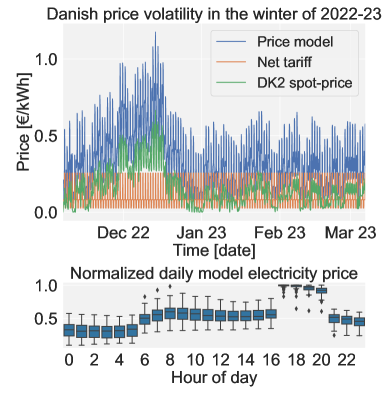
Figure 1: Upper: The Nord Pool market spot price plotted together with the Danish tariff Model 3.0. The price model is used for the economical evaluation of the experiment. Lower: The normalized ($x_{i}/\max(x)$) daily price development of the price model.

One such opportunity is to utilize a price-aware controller to load shift by boosting heat production (charge) in low cost periods and decrease (discharge) in high cost periods either with help of an energy storage [kelly_performance_2014, bechtel_influence_2020] or directly using the thermal mass of the building itself [amato_dual-zone_2023, sanchez_ramos_potential_2019, hu_price-responsive_2019]. A variable-speed heat pump can be used to boost heat by increasing the compressor speed, but this comes with a significant loss of efficiency (coefficient of performance, COP). Further, the COP of an air-to-water HP is highly dependent on ambient temperature, which means that not only price but also weather factors need to be considered as well.

A method suitable for automating heat load shifting is Model Predictive Control (MPC) [amato_dual-zone_2023]. During the last 30 years, MPC has been studied extensively in the context of building control due to its structural ability to integrate building dynamics, heating system and environmental aspects into an optimal control problem (OCP) formulation capable of handling both constraints and discrete states. A range of different versions of MPC have been suggested: Deterministic MPC, Stochastic MPC, Robust MPC, Learning MPC, Offset-free MPC, Implicit MPC and Explicit MPC [drgona_all_2020]. While the studies are numerous, the method has so far failed to make a broad impact on the space heating sector. The reported reasons are installation costs of sensor and actuators, model development costs [sturzenegger_model_2016] and user-acceptance.

Although the number of long term (beyond 30 days) building scale demonstrations are few compared to simulation studies, a selection of noteworthy examples do exist. In [sturzenegger_model_2016] a 6000 ${\mathrm{m}}^{2}$, occupied office building in Switzerland both in periods during winter and summer which combined into about 30 weeks of testing. While reporting that the control itself was a success, the author questions whether the method is mature enough to be implemented in similar buildings. In [de_coninck_practical_2016] two heat pumps and a gas boiler were controlled in a 960 ${\mathrm{m}}^{2}$ occupied office building in Brussels during the winter of 2014-2015 reporting cost savings of 30% while improving comfort. In Halifax, Canada, a 10000 ${\mathrm{m}}^{2}$ university building was controlled using MPC for four months with reported savings of 29% electricity and 63% heat [hilliard_experimental_2017]. In the category single-family houses, [pedersen_central_2013] controlled four houses for 5 months and reported an average cost reduction of 9% when compared to 7 benchmark houses and in [muller_large-scale_2019] HPs in 300 homes were ON/OFF throttled to reduce peak loads. The low number of residential experiments is likely due to the low potential for savings, which disqualifies large implementation costs. The requirement for simple solutions have spurred a branch of low-complexity MPC e.g. with only one central heat meter as in [amato_dual-zone_2023]. Recent studies [amato_dual-zone_2023, vogler-finck_inverse_2019] have demonstrated the basic feasibility of such schemes, but both studies point out that longer evaluation periods are needed to reliably verify their practical usefulness. Furthermore, occupancy in single-family houses is a fundamentally different condition from office buildings due to the invasive nature of sensor feedback on the occupants´ behavior, which must also be addressed.

Our contribution in this paper is a 97 day long study demonstrating a price responsive, low-complexity, hierarchical Mixed-Integer MPC control scheme on an occupied single-family house featuring an air-to-water heat pump and floor heating (FH). The controller is designed to minimize costs by shifting heating loads according to the electricity price signal together with other predictable and/or measurable factors. The controller is developed as a comparably low-complexity solution which only makes use of an internet connected control unit, a central heat meter, electricity meters, and room thermostats. Further, the weather forecast is provided by a weather service and the model is a single zone model which is based on a weighted average room temperature for the entire house. The controller is deliberately designed not to make use of explicit occupancy information, in order to protect the occupants´ right to privacy. The main findings from the experiment are: the near zero emission house demonstrated a high level of flexibility with respect to time-of-heating. Further, it is possible to boost the floors with heat during intensive sun radiation periods (when there is plenty of own-produced PV electricity) without further deteriorating the comfort. Controlling the upper layer using an area weighted average building temperature has shown to be unproblematic with respect to comfort in the test house.

The layout for the rest of the paper is as follows. Section 2 presents the case, an overview of the heating side and the electrical side viewed from a control perspective. Section 3 presents the hierarchical control strategy, starting with the supervisory controller and followed by the mid-level controllers. Section LABEL:sec_model contains the models used in the paper. Section LABEL:sec_experiment describes the experiment before the results are presented in Section LABEL:sec_results. As the results are based on real data, Section LABEL:sec_result_interpret is dedicated to the authors’ interpretation of the results. Finally, a common discussion section followed by conclusion in Sections LABEL:sec_discussion and LABEL:sec_conclusion, respectively.

2 System

This section starts with an introduction to the case followed by an overview of the heating system and electrics before delving into the control retro-fit. The relevant signals are listed in Table 1.

2.1 Case study

The case is a $230\text{\,}{\mathrm{m}}^{2}$, two-story single-family house from 2018; see Fig. 2. According to the Danish building regulation, it is classified as a low energy class building (BR2020), which, among other requirements, implies a maximum annual heat demand of $20\text{\,}\mathrm{kW}\text{\,}\mathrm{h}\text{\,}{\mathrm{m}}^{-2}$ [br18]. It is located on Sjælland (Zealand) in Denmark, with a south view over the sea. A south facing photovoltaic system is placed on the roof with a measured peak output of $4\text{\,}\mathrm{kW}$ in end of December and $5.5\text{\,}\mathrm{kW}$ in June. Space heating and domestic hot water is provided by a Bosch Compress 6000AW (air-to-water) heat pump with a nominal capacity of $7\text{\,}\mathrm{kW}$. Domestic hot water takes priority over space heating. Based on measured data the nominal electric consumption ranges from $200\text{\,}\mathrm{W}$ to $2500\text{\,}\mathrm{W}$. Floor heating, embedded in concrete, is installed throughout the house. The floor heating system is controlled by a Wavin controller and consists of 15 circuits delivering heat to 11 heating zones. Each zone has one thermostat assigned, meaning that if more circuits are supplying the same zone all valves in the particular zone opens when heat is requested. The circuits are ON/OFF controlled based on deviations from the temperature reference provided for each zone. The heat pump is controlled by an ambient temperature compensated heat curve. The household has a variable electricity price contract, which is based on the Nord Pool market spot-price.

Table 1: Relevant signals

Variable	Unit	Description
$\dot{Q}_{\text{HP}}$	$[$\mathrm{W}$]$	Heat flow output from HP
$Q_{\text{HP}}$	$[$\mathrm{kW}\text{\,}\mathrm{h}$]$	Heat output from HP
$P_{\text{HP}}$	$[$\mathrm{W}$]$	Electric power input to HP
$E_{\text{HP}}$	$[$\mathrm{kW}\text{\,}\mathrm{h}$]$	Electric energy input to HP
$P_{\text{PV}}$	$[$\mathrm{W}$]$	Electric power output from photovoltaic
$P_{\text{G}}$	$[$\mathrm{W}$]$	Electric power from grid
$P_{\text{APP}}$	$[$\mathrm{W}$]$	Household electric power consumption
$T_{\text{R}}$	$[$\mathrm{\SIUnitSymbolCelsius}$]$	Return temperature to HP
$T_{\text{R},i}$	$[$\mathrm{\SIUnitSymbolCelsius}$]$	Return Temperature from FH circuit $i$
$T_{\text{r},j}$	$[$\mathrm{\SIUnitSymbolCelsius}$]$	Air temperature in room $j$
$T_{\text{r},\lx@mung@bibliography@pre\thebibliography\lx@bibitem{,}j}$	$[$\mathrm{\SIUnitSymbolCelsius}$]$	Reference temp. in room $j$
$T_{\text{f},j}$	$[$\mathrm{\SIUnitSymbolCelsius}$]$	Estimated floor temperature in room $j$
$v_{i}$	$[$\mathrm{\SIUnitSymbolCelsius}$]$	ON/OFF Valve setting for circuit $i$
$q$	$[$\mathrm{kg}\text{\,}{\mathrm{s}}^{-1}$]$	Total flow into the FH system
$\mathcal{U}_{\text{a}}$	$[$\mathrm{V}$]$	Output voltage from ambient temperature sensor

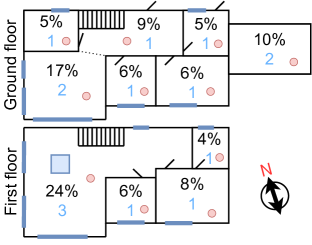
Figure 2: Blueprint of the floor plan with area distribution. Blue numbers indicate the number of FH circuits in each zone. Red circles show the presence of a room thermostat.

2.2 Heating system

Fig. 3 shows the heating system with associated signals. Note that heat flow to the floor heating system, $\dot{Q}_{\text{HP}}$, and electric power consumption of the heat pump, $P_{\text{HP}}$, are measured.

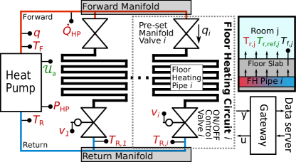
Figure 3: The diagram of the heating system in the house. The colors represent the kind of signal: red for measured variables, green for control inputs and black for estimated variables. Pipes on warm side are red and cold side blue.

The HP feeds the floor heating system with water, which in turn deliver the heat to the heating zones.

2.3 Electricity

The household electric grid is shown in Figure 4. The main units are photovoltaic panels and the heat pump which have separate electricity meters. The other household appliances are aggregated into an unknown disturbance.

Figure 4: The internal electricity grid of the house expressed in power. Red variables are measured quantities.

2.4 Retrofit architecture

The retrofit architecture, which is built and implemented by Neogrid Technologies, is seen in Fig. 5.

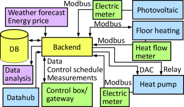
Figure 5: Shows the overview of the hardware and communication protocols. Blue color is for preinstalled hardware, green for installed sensors, yellow is the off-site infrastructure and purple are data services.

The infrastructure consists of an onsite part and a backend with the control box acting as gateway between them. The backend is responsible for refining, organizing, downloading data from weather and price services, and storing data, which is used for analysis and model fitting. The control box is responsible for providing control signals and collecting measurements from all units. In this case, it means to provide the artificial ambient temperature overwrite, via a digital to analog converter (DAC) and blocking the compressor using a relay. The datahub (Eloverblik) is an online platform, provided by the danish publicly owned company Energinet, where electricity-customers can get an overview of their consumption or share data with third-party. We use the BACnet and Modbus protocols to communicate with the floor heating controller for collecting room temperatures and other data from the floor heating system, and sending set-points to the valves.

2.5 Object oriented description of commercial domestic heat pump

In this section common properties for commercial air-to-water HP’s are listed together with references to how they are modelled in the literature.

1. ON/OFF indicator: the HP turns off when heat demand is absent. In this work the indicator variable $\delta_{\text{HP}}\in\{0,1\}$ is one when the HP is ON and zero if OFF [lee_mixed-integer_2019, mayer_management_2015].

2. Minimum load: the minimum load and operation range of a variable speed HP is often considered and modelled as a set $P_{\text{HP}}\in\{0\}\cup[\underline{P_{\text{HP}}},\overline{P_{\text{HP}}}]$ [kuboth_economic_2019, lee_mixed-integer_2019, maier_assessing_2022].

3. Coefficient of performance: the coefficient of performance (COP) is the ratio between the produced heat and consumed input energy (here electricity). It is often modelled as a static function, $f_{\text{HP}}:\mathbb{R}\to\mathbb{R}$.

4. Down-time: to avoid start-up cycling some HPs feature a (sometimes adaptive) down-time period measured in hours. To incorporate this a model for minimum up- and down-time can be included [mayer_management_2015, lohr_mpc_2021].

5. Limit on rate off change: the internal controllers of a domestic HP sometimes prevent it from changing state too rapidly.

6. Domestic hot water production: the HP switches between providing space heat and domestic hot water. Domestic hot water is often prioritized.

7. Discrete compressor speed steps: the compressor speed is often operated at certain steps rather than continuous action. Some speeds are excluded as resonance with the casing can cause noise.

8. Low pass filter on ambient temperature signal: it is common practice that commercial HPs apply a low pass filter to the ambient temperature signal before it is provided to the internal controllers.

9. Defrosting: an air-to-water HP needs to defrost the evaporator regularly in order to function properly. This event is treated as a random process which takes priority.

It is desirable that any MPC operating an HP can handle the listed properties.

3 Control

The control objective is to provide the required comfort level at the lowest cost feasible. To accomplish this, the controller needs to make two high-level control actions. First, it must choose the heat pump heat flow $\dot{Q}_{\text{HP}}(t)\in\mathbb{R}$ and the FH water flow $q(t)\in\mathbb{R}$. Second, it must guide the water to the most suitable rooms. It is not possible to control the heat and water flow directly, but it is possible to influence them indirectly. The heat production can be indirectly controlled using ambient temperature $T_{\text{a}}$, and valve positions $v$ affect flow:

$$\dot{Q}_{\text{HP}}(t)=f(T_{\text{a}},\cdot),\hskip 8.5359ptq=g(v,\cdot),\hskip 5.69046ptv\in\mathbb{R}^{N},\hskip 5.69046ptT_{\text{a}}\in\mathbb{R}$$ (1)

The $(\cdot,\cdot)$ notation indicates that heat and water flow are not only functions of ambient temperature and valve positions, but other factors too.

3.1 Control hierarchy

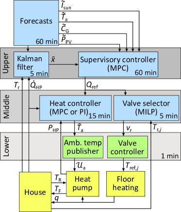
Figure 6: Shows the control diagram with signals. Blue indicates computations conducted remotely and green indicates onsite units and yellow the physical components. The grey boxes contain the control layers in the hierarchical control structure. The update period is shown in the modules.

The control concept comprises three control levels, see Fig. 6. The upper layer contains the supervisory controller that is aware of energy assets connected to the system as well as important externalities such as weather and electricity prices. It treats the energy assets as objects with properties which can be utilized for optimal control. A key feature of the supervisory controller is that it knows what the energy assets can do, and why they should do it, but not how to make them do it. The middle layer is tasked with tracking the heat reference, delivered by the supervisory controller, and distributing the heat to appropriate rooms. This layer knows how to deliver the demanded energy, but not why it does it. Based on the heat reference and room temperatures, the valve selector chooses the valves to be opened in order to provide a flow, which works as an operating point for the heat controller, and to transport the heat to the rooms that need it the most. The heat controller follows the heat reference by providing an artificial ambient temperature to the ambient temperature publisher to indirectly control the compressor speed.

The lowest layer handles the interface between the control signal and the actual hardware. The ambient temperature publisher translates the artificial ambient temperature provided by the heat controller to a voltage which emulates the outdoor temperature sensors output at given temperature. The valve controller translates the valve-selection into room temperature references designed to force circuits open or closed.

3.2 Supervisory controller

Fig. 7 presents the concept for the supervisory controller in the upper layer.

Figure 7: Overview of the top layer supervisory controller.

The controller relies on three main components, forecasts, models and measurements. Based on these, the controller computes a heat reference (or “budget”), $Q_{\lx@mung@bibliography@pre\thebibliography\lx@bibitem{}}$, which is dispatched to the lower level controllers. The hierarchical structure makes the supervisory controller more flexible than a monolithic structure, since it can calculate the heat reference without concern for how the heat is delivered—it just needs to know at which efficiency and rate the heat can be delivered. The biggest drawback of using heat for the interface is that it needs to be measured, and adding a heat flow sensor to the hydraulic network is costly.

3.2.1 Design of supervisory controller

The conceptualized version of the Mixed Integer Optimal Control Problem (MIOCP) at the core of the Mixed Integer Model Predictive Control (MIMPC) is seen in equation system (2) on a form which describes the functionality of the cost and various constraints rather than the implementation. Note that (2) contains two sub-versions decided by the indicator variable $\delta_{\text{OP}}$. It must be stressed that the value of $\delta_{\text{OP}}$ is chosen before implementing the problem, it is not an optimization variable (in this case study: $\delta_{\text{OP}}=1$). The difference between the two versions is the HP efficiency model.

$$J(u_{\text{OP}}^{*})=\min_{u_{\text{OP}}}f_{\text{G}}(P_{\text{G}})+f_{\text{CO}_{2}}(P_{\text{G}})+f_{\text{cmf}}(T_{\text{r}},T_{\text{r},\lx@mung@bibliography@pre\thebibliography\lx@bibitem{}})$$ (2a)

$$u_{\text{OP}}=\begin{cases}(P_{\text{HP}},\delta_{\text{HP}},S)&\delta_{\text{OP}}=1\\ (\dot{Q}_{\text{HP}},\delta_{\text{HP}},S)&\delta_{\text{OP}}=0\end{cases}$$ (2b)

$$u_{\text{OP}}\in\mathbb{R}^{N}\times\{0,1\}^{N}\times\mathbb{R}^{N_{\text{s}}}_{+}$$ (2c)

s.t.

$$P_{\text{G}}=P_{\text{HP}}-\tilde{P}_{\text{PV}}+P_{\text{APP}}$$ (2d)

$$\mathbf{x}_{i+1}=\mathbf{A}\mathbf{x}_{i}+\mathbf{B}\dot{Q}_{\text{HP},i}+\mathbf{E}\mathbf{d}_{i},\hskip 14.22636ptT_{\text{r},i}=\mathbf{C}\mathbf{x}_{i}$$ (2e)

$$\text{if}\hskip 5.69054pt\delta_{\text{OP}}=1\hskip 5.69054pt\text{then}\hskip 5.69054pt\dot{Q}_{\text{HP},i}=f_{\text{HP},\dot{Q}}(P_{\text{HP},i},T_{\text{a},i})\delta_{\text{HP},i}$$ (2f)

$$\text{if}\hskip 5.69054pt\delta_{\text{OP}}=0\hskip 5.69054pt\text{then}\hskip 5.69054ptP_{\text{HP},i}=f_{\text{HP},P}(\dot{Q}_{\text{HP},i},T_{\text{a},i})\delta_{\text{HP},i}$$ (2g)

$$P_{\text{HP},i}\in\begin{cases}[\underline{P_{\text{HP}}},\overline{P_{\text{HP}}}]&\delta_{\text{HP},i}=1\\ 0&\delta_{\text{HP},i}=0\end{cases}$$ (2h)

$$\Delta\delta_{\text{HP},i}=\delta_{\text{HP},i}-\delta_{\text{HP},i-1}\hskip 8.5359pt\Delta P_{\text{HP},i}=P_{\text{HP},i}-P_{\text{HP},i-1}$$ (2i)

$$\Delta P_{\text{HP},i}\in\begin{cases}[\Delta\underline{P_{\text{HP}}},\Delta\overline{P_{\text{HP}}}]&\delta_{\text{HP},i}=1\\ (-\infty,\Delta\overline{P_{\text{HP}}}]&\delta_{\text{HP},i}=0\end{cases}$$ (2j)

$$\Delta\delta_{\text{HP},i}=-1\implies\delta_{\text{HP},i+1},\dots,\delta_{\text{HP},i+M-1}=0$$ (2k)

The cost function is the sum of three functions. First, a linear term, $f_{\text{G}}(P_{\text{G}})$, describing the differentiated cost of either importing from or exporting to the electricity grid. The input is consumed electricity from the grid, $P_{\text{G}}$, with positive values indicating import. The prices for buying and selling to the grid are given as $c_{\text{E}}^{+}>0$ and $c_{\text{E}}^{-}>0$, respectively. The second term is a self-imposed $\text{CO}_{2}$-tax. The third is the comfort term which punishes deviations from the desired temperature. Slack variables are used to ensure feasibility. Together the terms make out a convex cost-function.

The constraint (2d) describes the electricity balance were the amount of electricity bought from the grid (G) is calculated. Constraint (2e) describes the linear dynamics of the house. Constraints (2f)-(2k) models the properties of the HP presented in Section 2.5. Constraints (2f) and (2g) both describes the HP efficiency, but only one is active dependent on the initial choice of $\delta_{\text{OP}}$. Constraint (2h) describes the piece-wise function where the compressor either is off, or operating in the range $[\underline{P_{\text{HP}}},\overline{P_{\text{HP}}}]$. The constraint (2j) limits the rate off change between control periods. To meet the requirement that the HP can be turned off from any operational state, the down rate is set to $-\infty$ when $\delta_{\text{HP},i}=0$. Last (2k) forces the HP to stay turned off for minimum $M$ sample times. Having described the functionality of the optimization problem  the next part focuses on implementation aspects.

The guiding principle for the implementation is that the structure of the problem is convex if the problem is relaxed, meaning that if integer variables are replaced with continuous ones, the problem is convex. The cost function from equation system(2) is implemented as:

$$J(u_{\text{OP}})=c_{\text{E}}^{-\text{T}}P_{\text{G}}+\Delta c_{\text{E}}^{+\text{T}}P_{\text{G}}^{+}+z_{\text{cmf}}+c_{\text{s}}^{T}S$$ (3)

Here the auxiliary variables $P_{\text{G}}^{+},z_{\text{cmf}}\in\mathbb{R}^{N}_{+}$ are introduced. The variable $P_{\text{G}}^{+}$ is defined as entry-wise $\max(0,P_{\text{G}})$ and $z_{\text{cmf}}$ has to be larger than any competing comfort constraints. The vector $\Delta c_{\text{E}}^{+}=c_{\text{E}}^{+}-c_{\text{E}}^{-}>0$ describes the positive difference between buying price and selling price. Note that the buying price needs to be higher than the selling price, otherwise the solution to the optimization problem entails buying excessive amounts of electricity just to sell it again in the same instance. The auxiliary variable $z_{\text{cmf}}$ encodes the expression $\max(f_{\text{cmf},1}(T_{\text{r}},T_{\text{r},\lx@mung@bibliography@pre\thebibliography\lx@bibitem{}}),\cdots,f_{\text{cmf},N_{\text{cmf}}}(T_{\text{r}},T_{\text{r},\lx@mung@bibliography@pre\thebibliography\lx@bibitem{}}))$ where $f_{\text{cmf},i}(T_{\text{r}},T_{\text{r},\lx@mung@bibliography@pre\thebibliography\lx@bibitem{}})$ with $i\in\{1,...,N_{\text{cmf}}\}$ is either an affine or quadratic positive definite function. This formulation gives room for skewed functions which can for instance penalize either over- or under-heating. Note that the artificial $\text{CO}_{2}$-tax term is not missing, it is merely incorporated into the buying price as described in Section LABEL:sec_price_model.

The HP efficiency model in either (2g) or (2f) is implemented using the known Mixed Logic Dynamics technique from [bemporad_control_1999] where an auxiliary variable is introduced $z_{\text{HP},i}$ to either be zero of mirror the value of the function dependent on $\delta_{\text{HP},i}$. To preserve convexity of the input set, only an inequality is used instead of the original equality seen in (2g). if $\delta_{\text{OP}}=0$ then $P_{\text{HP},i}\geq f_{\text{HP},P}(\dot{Q}_{\text{HP},i},T_{\text{a},i})$ and if $\delta_{\text{OP}}=0$ then $\dot{Q}_{\text{HP},i}\leq f_{\text{HP},\dot{Q}}(P_{\text{HP},i},T_{\text{a},i})\delta_{\text{HP},i}$. The structure of the problem forces the solution onto the curve emulating the equality constraint. When $\delta_{\text{OP}}=1$, there are a few cases where $\dot{Q}_{\text{HP}}$ deviates from the curve to avoid the cost of overheating. To avoid this an equality constraint can be implemented with the added computational cost. The constraint in (2h) is implemented as e.g. in [kuboth_economic_2019, lee_mixed-integer_2019, parisio_model_2014], so is the constraint in (2j). The down-time model constraint in (2k) can be implemented as shown in [parisio_model_2014]. The problem can be summed up to

$$\min_{\mathbf{u}\in\mathbb{R}^{m\times N},}J(\mathbf{x}_{0},\mathbf{u})$$ (4a)

s.t. (4b)

$$\mathbf{x}_{k+1}=\mathbf{A}\mathbf{x}_{k}+\mathbf{B}\mathbf{u}_{k}+\mathbf{E}\mathbf{d}_{k},\hskip 5.69046pt\mathbf{x}_{k}\in\mathcal{X},\hskip 5.69046pt\mathbf{x}_{0}=\mathbf{x}(t)$$ (4c)

$$\mathbf{y}_{1,k}=\mathbf{C}\mathbf{x}_{k}+\mathbf{D}\mathbf{u}_{k},\hskip 5.69046pt\mathbf{u}_{k}\in\mathcal{U}$$ (4d)

$$\mathbf{y}_{2,k}\geq\textbf{f}_{\text{convex}}(\mathbf{x}_{k},\mathbf{u}_{k})\hskip 17.07182pt\mathbf{y}_{3,k}\leq\textbf{f}_{\text{concave}}(\mathbf{x}_{k},\mathbf{u}_{k})$$ (4e)

where $J$ is the convex cost function. Section LABEL:sec_model details the models that specify the MPC formulation given here.

3.3 Valve selector

The valve selector, or dispatcher, is a mixed integer linear programming problem tasked with providing the flow, $q$, as requested, $q_{\lx@mung@bibliography@pre}\thebibliography\lx@bibitem{$},anddistributethewatertothemostsuitablerooms.NotethattheValveselectorisonlyreactivecontrol.Theoptimizationproblemis\lx@equationgroup@subnumbering@begin\begin{aligned} &\min_{v\in\{0,1\}^{M}}J(v)=\min_{v\in\{0,1\}^{M}}c_{q}\|q_{\lx@bibitem{-}}q\|^{2}_{2}+c_{\text{cmf}}^{\text{T}}v\vspace{0mm}\\ &\text{s.t.}\vspace{0mm}\\ &\overline{q}=\sum_{i=1}^{M}v_{i}\overline{q}_{i},\vspace{0mm}\\ &q=c_{0}+c_{1}\overline{q}+c_{2}\overline{q}^{2}\vspace{0mm}\\ &q\geq q_{\min},\vspace{0mm}\\ &r_{m}\geq\sum_{i=1}^{M}\max(v_{0,i}-v_{i},0),\vspace{0mm}\\ &v_{j}=1,\hskip 28.45274pt\forall j\in\mathcal{J}.\end{aligned}\lx@equationgroup@subnumbering@end Thecostfunctionisatrade-offbetweenfollowingtheflowreferenceanddeliveringtheheattotherightrooms.Thetwotermsareweightedby$c_$q$ ∈R_+$and$$c_{\text{cmf}}$∈$\mathbb{R}^{N_{\text{r}}}$$.Thecomfortcostispre-calculatedas$$c_{\text{cmf},i}$ = a($T_{\text{r},i}$ - $T{}_{\text{r},}$