Your Diffusion Model is Secretly a Zero-Shot Classifier

Abstract

The recent wave of large-scale text-to-image diffusion models has dramatically increased our text-based image generation abilities. These models can generate realistic images for a staggering variety of prompts and exhibit impressive compositional generalization abilities. Almost all use cases thus far have solely focused on sampling; however, diffusion models can also provide conditional density estimates, which are useful for tasks beyond image generation. In this paper, we show that the density estimates from large-scale text-to-image diffusion models like Stable Diffusion can be leveraged to perform zero-shot classification without any additional training. Our generative approach to classification, which we call Diffusion Classifier, attains strong results on a variety of benchmarks and outperforms alternative methods of extracting knowledge from diffusion models. Although a gap remains between generative and discriminative approaches on zero-shot recognition tasks, our diffusion-based approach has significantly stronger multimodal compositional reasoning ability than competing discriminative approaches. Finally, we use Diffusion Classifier to extract standard classifiers from class-conditional diffusion models trained on ImageNet. Our models achieve strong classification performance using only weak augmentations and exhibit qualitatively better “effective robustness” to distribution shift. Overall, our results are a step toward using generative over discriminative models for downstream tasks. Results and visualizations on our website: diffusion-classifier.github.io/

1 Introduction

To Recognize Shapes, First Learn to Generate Images [31]—in this seminal paper, Geoffrey Hinton emphasizes generative modeling as a crucial strategy for training artificial neural networks for discriminative tasks like image recognition. Although generative models tackle the more challenging task of accurately modeling the underlying data distribution, they can create a more complete representation of the world that can be utilized for various downstream tasks. As a result, a plethora of implicit and explicit generative modeling approaches [26, 42, 46, 21, 77, 70, 79] have been proposed over the last decade. However, the primary focus of these works has been content creation [18, 8, 39, 40, 76, 34] rather than their ability to perform discriminative tasks. In this paper, we revisit this classic generative vs. discriminative debate in the context of diffusion models, the current state-of-the-art generative model family. In particular, we examine how diffusion models compare against the state-of-the-art discriminative models on the task of image classification.

Diffusion models are a recent class of likelihood-based generative models that model the data distribution via an iterative noising and denoising procedure [70, 35]. They have recently achieved state-of-the-art performance [20] on several text-based content creation and editing tasks [24, 67, 34, 66, 59]. Diffusion models operate by performing two iterative processes—the fixed forward process, which destroys structure in the data by iteratively adding noise, and the learned backward process, which attempts to recover the structure in the noised data. These models are trained via a variational objective, which maximizes an evidence lower bound (ELBO) [5] of the log-likelihood. For most diffusion models, computing the ELBO consists of adding noise $\epsilon$ to a sample, using the neural network to predict the added noise, and measuring the prediction error.

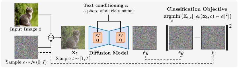
Figure 1: Overview of our Diffusion Classifier approach: Given an input image $\mathbf{x}$ and a set of possible conditioning inputs (e.g., text for Stable Diffusion or class index for DiT, an ImageNet class-conditional model), we use a diffusion model to choose the one that best fits this image. Diffusion Classifier is theoretically motivated through the variational view of diffusion models and uses the ELBO to approximate $\log p_{\theta}(\mathbf{x}\mid\mathbf{c})$. Diffusion Classifier chooses the conditioning $\mathbf{c}$ that best predicts the noise added to the input image. Diffusion Classifier can be used to extract a zero-shot classifier from Stable Diffusion and a standard classifier from DiT without any additional training.

Conditional generative models like diffusion models can be easily converted into classifiers [54]. Given an input $\mathbf{x}$ and a finite set of classes $\mathbf{c}$ that we want to choose from, we can use the model to compute class-conditional likelihoods $p_{\theta}(\mathbf{x}\mid\mathbf{c})$. Then, by selecting an appropriate prior distribution $p(\mathbf{c})$ and applying Bayes’ theorem, we can get predicted class probabilities $p(\mathbf{c}\mid\mathbf{x})$. For conditional diffusion models that use an auxiliary input, like a class index for class-conditioned models or prompt for text-to-image models, we can do this by leveraging the ELBO as an approximate class-conditional log-likelihood $\log p(\mathbf{x}\mid\mathbf{c})$. In practice, obtaining a diffusion model classifier through Bayes’ theorem consists of repeatedly adding noise and computing a Monte Carlo estimate of the expected noise reconstruction losses (also called $\epsilon$-prediction loss) for every class. We call this approach Diffusion Classifier. Diffusion Classifier can extract zero-shot classifiers from text-to-image diffusion models and standard classifiers from class-conditional diffusion models, without any additional training. We develop techniques for appropriately choosing diffusion timesteps to compute errors at, reducing variance in the estimated probabilities, and speeding up classification inference.

We highlight the surprising effectiveness of our proposed Diffusion Classifier on zero-shot classification, compositional reasoning, and supervised classification tasks by comparing against multiple baselines on eleven different benchmarks. By utilizing Stable Diffusion [65], Diffusion Classifier achieves strong zero-shot accuracy and outperforms alternative approaches for extracting knowledge from the pretrained diffusion model. Our approach also outperforms the strongest contrastive methods on the challenging Winoground compositional reasoning benchmark [75]. Finally, we use our approach to perform standard classification with Diffusion Transformer (DiT), an ImageNet-trained class-conditional diffusion model. Our generative approach achieves 79.1% accuracy on ImageNet using only weak augmentations and exhibits better robustness to distribution shift than competing discriminative classifiers trained on the same dataset. Our results suggest that it may be time to revisit generative approaches to classification.

2 Related Work

Generative Models for Discriminative Tasks:

Machine learning algorithms designed to solve common classification or regression tasks generally operate under two paradigms: discriminative approaches directly learn to model the decision boundary of the underlying task, while generative approaches learn to model the distribution of the data and then address the underlying task as a maximum likelihood estimation problem. Algorithms like naive Bayes [54], VAEs [42], GANs [26], EBMs [23, 46], and diffusion models [70, 35] fall under the category of generative models. The idea of modeling the data distribution to better learn the discriminative feature has been highlighted by several seminal works [31, 54, 63]. These works train deep belief networks [32] to model the underlying image data as latents, which are later used for image recognition tasks. Recent works on generative modeling have also learned efficient representations for both global and dense prediction tasks like classification [28, 33, 13, 8, 19] and segmentation [47, 83, 10, 3, 9]. Moreover, such models [27, 51, 37] have been shown to be more adversarially robust and better calibrated. However, most of the aforementioned works either train jointly for discriminative and generative modeling or fine-tune generative representations for downstream tasks. Directly utilizing generative models for discriminative tasks is a relatively less-studied problem, and in this work, we particularly highlight the efficacy of directly using recent diffusion models as image classifiers.

Diffusion Models:

Diffusion models [35, 70] have recently gained significant attention from the research community due to their ability to generate high-fidelity and diverse content like images [67, 55, 24], videos [69, 34, 78], 3D [59, 50], and audio [43, 52] from various input modalities like text. Diffusion models are also closely tied to EBMs [46, 23], denoising score matching [72, 80], and stochastic differential equations [73, 84]. In this work, we investigate to what extent the impressive high-fidelity generative abilities of these diffusion models can be utilized for discriminative tasks (namely classification). We take advantage of the variational view of diffusion models for efficient and parallelizable density estimates. The prior work of Dhariwal & Nichol [20] proposed using a classifier network to modify the output of an unconditional generative model to obtain class-conditional samples. Our goal is the reverse: using diffusion models as classifiers.

Zero-Shot Image Classification:

Classifiers thus far have usually been trained in a supervised setting where the train and test sets are fixed and limited. CLIP [61] showed that exploiting large-scale image-text data can result in zero-shot generalization to various new tasks. Since then, there has been a surge toward building a new category of classifiers, known as zero-shot or open-vocabulary classifiers, that are capable of detecting a wide range of class categories [25, 48, 49, 1]. These methods have been shown to learn robust representations that generalize to various distribution shifts [38, 16, 74]. Note that in spite of them being called “zero-shot,” it is still unclear whether evaluation samples lie in their training data distribution. In contrast to the discriminative approaches above, we propose extracting a zero-shot classifier from a large-scale generative model.

3 Method: Classification via Diffusion Models

We describe our approach for calculating class conditional density estimates in a practical and efficient manner using diffusion models. We first provide an overview of diffusion models (Sec. 3.1), discuss the motivation and derivation of our Diffusion Classifier method (Sec. 3.2), and finally propose techniques to improve its accuracy (Sec. 3.3).

3.1 Diffusion Model Preliminaries

Diffusion probabilistic models (“diffusion models” for short) [70, 35] are generative models with a specific Markov chain structure. Starting at a clean sample $\mathbf{x}_{0}$, the fixed forward process $q(\mathbf{x}_{t}\mid\mathbf{x}_{t-1})$ adds Gaussian noise, whereas the learned reverse process $p_{\theta}(\mathbf{x}_{t-1}\mid\mathbf{x}_{t},\mathbf{c})$ tries to denoise its input, optionally conditioning on a variable $\mathbf{c}$. In our setting, $\mathbf{x}$ is an image and $\mathbf{c}$ represents a low-dimensional text embedding (for text-to-image synthesis) or class index (for class-conditional generation). Diffusion models define the conditional probability of $\mathbf{x}_{0}$ as:

$$p_{\theta}(\mathbf{x}_{0}\mid\mathbf{c})=\int_{\mathbf{x}_{1:T}}p(\mathbf{x}_{T})\prod_{t=1}^{T}p_{\theta}(\mathbf{x}_{t-1}\mid\mathbf{x}_{t},\mathbf{c})\ \mathrm{d}\mathbf{x}_{1:T}$$ (1)

where $p(\mathbf{x}_{T})$ is typically fixed to $\mathcal{N}(0,I)$. Directly maximizing $p_{\theta}(\mathbf{x}_{0})$ is intractable due to the integral, so diffusion models are instead trained to minimize the variational lower bound (ELBO) of the log-likelihood:

$$\log p_{\theta}(\mathbf{x}_{0}\mid\mathbf{c}) \geq\mathbb{E}_{q}\left[\log\frac{p_{\theta}(\mathbf{x}_{0:T},\mathbf{c})}{q(\mathbf{x}_{1:T}\mid\mathbf{x}_{0})}\right]$$ (2)

Diffusion models parameterize $p_{\theta}(\mathbf{x}_{t-1}\mid\mathbf{x}_{t},\mathbf{c})$ as a Gaussian and train a neural network to map a noisy input $\mathbf{x}_{t}$ to a value used to compute the mean of $p_{\theta}(\mathbf{x}_{t-1}\mid\mathbf{x}_{t},\mathbf{c})$. Using the fact that each noised sample $\mathbf{x}_{t}=\sqrt{\bar{\alpha}_{t}}\mathbf{x}+\sqrt{1-\bar{\alpha}_{t}}\epsilon$ can be written as a weighted combination of a clean input $\mathbf{x}$ and Gaussian noise $\epsilon\sim\mathcal{N}(0,I)$, diffusion models typically learn a network $\epsilon_{\theta}(\mathbf{x}_{t},\mathbf{c})$ that estimates the added noise. Using this parameterization, the ELBO can be written as:

$$-\mathbb{E}_{\epsilon}\left[\sum_{t=2}^{T}w_{t}\|\epsilon-\epsilon_{\theta}(\mathbf{x}_{t},\mathbf{c})\|^{2}-\log p_{\theta}(\mathbf{x}_{0}\mid\mathbf{x}_{1},\mathbf{c})\right]+C$$ (3)

where $C$ is a constant term that does not depend on $\mathbf{c}$. Since $T=1000$ is large and $\log p_{\theta}(\mathbf{x}_{0}\mid\mathbf{x}_{1},\mathbf{c})$ is typically small, we choose to drop this term. Finally, [35] find that removing $w_{t}$ improves sample quality metrics, and many follow-up works also choose to do so. We found that deviating from the uniform weighting used at training time hurts accuracy, so we set $w_{t}=1$. Thus, this gives us our final approximation that we treat as the ELBO:

$$-\mathbb{E}_{t,\epsilon}\left[\|\epsilon-\epsilon_{\theta}(\mathbf{x}_{t},\mathbf{c})\|^{2}\right]+C$$ (4)

Algorithm 1 Diffusion Classifier

1:  Input: test image $\mathbf{x}$, conditioning inputs $\{\mathbf{c}_{i}\}_{i=1}^{n}$ (e.g., text embeddings), # of trials $T$ per input

2:  Initialize $\texttt{Errors}[\mathbf{c}_{i}]=\text{list}()$ for each $\mathbf{c}_{i}$

3:  for trial $j=1,\dots,T$ do

4:     Sample $t\sim[1,1000]$;   $\epsilon\sim\mathcal{N}(0,I)$

5:     $\mathbf{x}_{t}=\sqrt{\bar{\alpha}_{t}}\mathbf{x}+\sqrt{1-\bar{\alpha}_{t}}\epsilon$

6:     for conditioning $\mathbf{c}_{k}\in\{\mathbf{c}_{i}\}_{i=1}^{n}$ do

7:        $\texttt{Errors}[\mathbf{c}_{k}].\texttt{append}(\|\epsilon-\epsilon_{\theta}(\mathbf{x}_{t},\mathbf{c}_{k})\|^{2})$

8:     end for

9:  end for

10:  return  $\displaystyle\operatorname*{arg\,min}_{\mathbf{c}_{i}\in\mathcal{C}}\texttt{\,mean}(\texttt{Errors}[\mathbf{c}_{i}])$

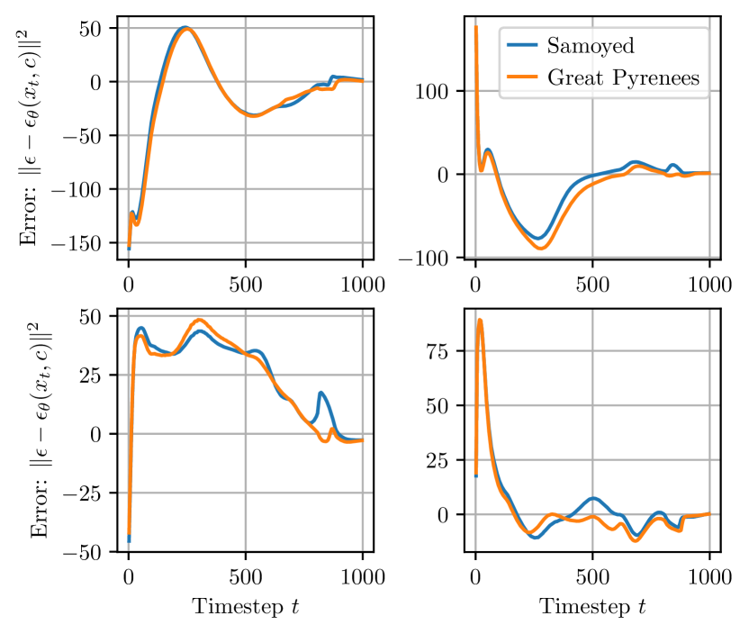
Figure 2: We show the $\epsilon$-prediction error for an image of a Great Pyrenees dog and two prompts (“Samoyed” and “Great Pyrenees”). Each subplot corresponds to a single $\epsilon_{i}$, with the error evaluated at every $t\in\{1,2,...,1000\}$. Errors are normalized to be zero-mean at each timestep across the 4 plots, and lower is better. Variance in $\epsilon$-prediction error is high across different $\epsilon$, but the variance in the error difference between prompts is much smaller.

3.2 Classification with diffusion models

In general, classification using a conditional generative model can be done by using Bayes’ theorem on the model predictions $p_{\theta}(\mathbf{x}\mid\mathbf{c}_{i})$ and the prior $p(\mathbf{c})$ over labels $\{\mathbf{c}_{i}\}$:

$$p_{\theta}(\mathbf{c}_{i}\mid\mathbf{x})=\frac{p(\mathbf{c}_{i})\ p_{\theta}(\mathbf{x}\mid\mathbf{c}_{i})}{\sum_{j}p(\mathbf{c}_{j})\ p_{\theta}(\mathbf{x}\mid\mathbf{c}_{j})}$$ (5)

A uniform prior over $\{\mathbf{c}_{i}\}$ (i.e., $p(\mathbf{c}_{i})=\frac{1}{N}$) is natural and leads to all of the $p(\mathbf{c})$ terms cancelling. For diffusion models, computing $p_{\theta}(\mathbf{x}\mid\mathbf{c})$ is intractable, so we use the ELBO in place of $\log p_{\theta}(\mathbf{x}\mid\mathbf{c})$ and use Eq. 4 and Eq. 5 to obtain a posterior distribution over $\{\mathbf{c}_{i}\}_{i=1}^{N}$:

$$p_{\theta}(\mathbf{c}_{i}\mid\mathbf{x}) =\frac{\exp\{-\mathbb{E}_{t,\epsilon}[\|\epsilon-\epsilon_{\theta}(\mathbf{x}_{t},\mathbf{c}_{i})\|^{2}]\}}{\sum_{j}\exp\{-\mathbb{E}_{t,\epsilon}[\|\epsilon-\epsilon_{\theta}(\mathbf{x}_{t},\mathbf{c}_{j})\|^{2}]\}}$$ (6)

We compute an unbiased Monte Carlo estimate of each expectation by sampling $N$ $(t_{i},\epsilon_{i})$ pairs, with $t_{i}\sim[1,1000]$ and $\epsilon\sim\mathcal{N}(0,I)$, and computing:

$$\frac{1}{N}\sum_{i=1}^{N}\left\|\epsilon_{i}-\epsilon_{\theta}(\sqrt{\bar{\alpha}_{t_{i}}}\mathbf{x}+\sqrt{1-\bar{\alpha}_{t_{i}}}\epsilon_{i},\mathbf{c}_{j})\right\|^{2}$$ (7)

By plugging Eq. 7 into Eq. 6, we can extract a classifier from any conditional diffusion model. We call this method Diffusion Classifier. Diffusion Classifier is a powerful, hyperparameter-free approach to extracting classifiers from pretrained diffusion models without any additional training. Diffusion Classifier can be used to extract a zero-shot classifier from a text-to-image model like Stable Diffusion [65], to extract a standard classifier from a class-conditional diffusion model like DiT [58], and so on. We outline our method in Algorithm 1 and show an overview in Figure 1.

3.3 Variance Reduction via Difference Testing

At first glance, it seems that accurately estimating $\mathbb{E}_{t,\epsilon}\left[\|\epsilon-\epsilon_{\theta}(\mathbf{x}_{t},\mathbf{c})\|^{2}\right]$ for each class $\mathbf{c}$ requires prohibitively many samples. Indeed, a Monte Carlo estimate even using thousands of samples is not precise enough to distinguish classes reliably. However, a key observation is that classification only requires the relative differences between the prediction errors, not their absolute magnitudes. We can rewrite the approximate $p_{\theta}(\mathbf{c}_{i}\mid\mathbf{x})$ from Eq. 6 as:

$$\frac{1}{\sum_{j}\exp\left\{\mathbb{E}_{t,\epsilon}[\|\epsilon-\epsilon_{\theta}(\mathbf{x}_{t},\mathbf{c}_{i})\|^{2}-\|\epsilon-\epsilon_{\theta}(\mathbf{x}_{t},\mathbf{c}_{j})\|^{2}]\right\}}$$ (8)

Eq. 8 makes apparent that we only need to estimate the difference in prediction errors across each conditioning value. Practically, instead of using different random samples of $(t_{i},\epsilon_{i})$ to estimate the ELBO for each conditioning input $\mathbf{c}$, we simply sample a fixed set $S=\{(t_{i},\epsilon_{i})\}_{i=1}^{N}$ and use the same samples to estimate the $\epsilon$-prediction error for every $\mathbf{c}$. This is reminiscent of paired difference tests in statistics, which increase their statistical power by matching conditions across groups and computing differences.

In Figure 2, we use 4 fixed $\epsilon_{i}$’s and evaluate $\|\epsilon_{i}-\epsilon_{\theta}(\sqrt{\bar{\alpha}_{t}}\mathbf{x}+\sqrt{1-\bar{\alpha}_{t}}\epsilon_{i},\mathbf{c})\|^{2}$ for every $t\in{1,\dots,1000}$, two prompts (“Samoyed dog” and “Great Pyrenees dog”), and a fixed input image of a Great Pyrenees. Even for a fixed prompt, the $\epsilon$-prediction error varies wildly across the specific $\epsilon_{i}$ used. However, the error difference between each prompt is much more consistent for each $\epsilon_{i}$. Thus, by using the same $(t_{i},\epsilon_{i})$ for each conditioning input, our estimate of $p_{\theta}(\mathbf{c}_{i}\mid\mathbf{x})$ is much more accurate.

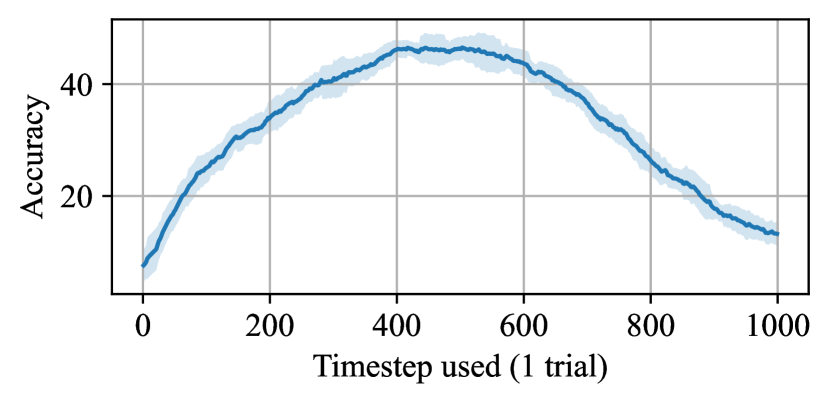
Figure 3: Pets accuracy, evaluating only a single timestep per class. Small $t$ corresponds to less noise added, and large $t$ corresponds to significant noise. Accuracy is highest when an intermediate amount of noise is added ($t=500$).

4 Practical Considerations

Our Diffusion Classifier method requires repeated error prediction evaluations for every class in order to classify an input image. These evaluations naively require significant inference time, even with the technique presented in Section 3.3. In this section, we present further insights and optimizations that reduce our method’s runtime.

4.1 Effect of timestep

Diffusion Classifier, which is a theoretically principled method for estimating $p_{\theta}(\mathbf{c}_{i}\mid\mathbf{x})$, uses a uniform distribution over the timestep $t$ for estimating the $\epsilon$-prediction error. Here, we check if alternate distributions over $t$ yield more accurate results. Figure 3 shows the Pets accuracy when using only a single timestep evaluation per class. Perhaps intuitively, accuracy is highest when using intermediate timesteps ($t\approx 500)$. This begs the question: can we improve accuracy by oversampling intermediate timesteps and undersampling low or high timesteps?

We try a variety of timestep sampling strategies, including repeatedly trying $t=500$ with many random $\epsilon$, trying $N$ evenly spaced timesteps, and trying the middle ${t-N/2,\dots,t+N/2}$ timesteps. The tradeoff between different strategies is whether to try a few $t_{i}$ repeatedly with many $\epsilon$ or to try many $t_{i}$ once. Figure 4 shows that all strategies improve when taking using average error of more samples, but simply using evenly spaced timesteps is best. We hypothesize that repeatedly trying a small set of $t_{i}$ scales poorly since this biases the ELBO estimate.

4.2 Efficient Classification

A naive implementation of our method requires $C\times N$ trials to classify a given image, where $C$ is the number of classes and $N$ is the number of $(t,\epsilon)$ samples to evaluate to estimate each conditional ELBO. However, we can do better. Since we only care about $\operatorname*{arg\,max}_{\mathbf{c}}p(\mathbf{c}\mid\mathbf{x})$, we can stop computing the ELBO for classes we can confidently reject. Thus, one option to classify an image is to use an upper confidence bound algorithm [2] to allocate most of the compute to the top candidates. However, this requires assuming that the distribution of $\|\epsilon-\epsilon_{\theta}(\mathbf{x}_{t},\mathbf{c}_{j})\|^{2}$ is the same across timesteps $t$, which does not hold.

We found that a simpler method works just as well. We split our evaluation into a series of stages, where in each stage we try each remaining $\mathbf{c}_{i}$ some number of times and then remove the ones that have the highest average error. This allows us to efficiently eliminate classes that are almost certainly not the final output and allocate more compute to reasonable classes. For example, on the Pets dataset, we have $N_{\text{stages}}$ = 2. We try each class 25 times in the first stage, then prune to the 5 classes with the smallest average error. Finally, in the second stage we try each of the 5 remaining classes 225 additional times. In Algorithm 2, we write this as $\texttt{KeepList}=(5,1)$ and $\texttt{TrialList}=(25,250)$. With this evaluation strategy, classifying one Pets image requires 18 seconds on a RTX 3090 GPU. As our work focuses on understanding diffusion model capabilities and not on developing a fully practical inference algorithm, we do not significantly tune the evaluation strategies. Further details on adaptive evaluation are in Appendix A.

Further reducing inference time could be a valuable avenue for future work. Inference is still impractical when there are many classes. Classifying a single ImageNet image, with 1000 classes, takes about 1000 seconds with Stable Diffusion at $512\times 512$ resolution, even with our adaptive strategy. Table 7 shows inference times for each dataset, and we discuss promising approaches for speedups in Section 7.

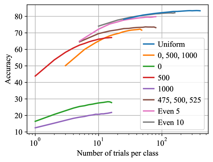
Figure 4: Zero-shot scaling curves for different timestep sampling strategies. We evaluate a variety of strategies for choosing the timesteps at which we evaluate the $\epsilon$-prediction error. Each strategy name indicates which timesteps it uses— e.g., “$0$” only uses the first timestep, “$0,500,1000$” uses only the first, middle and last, “Even 10” uses 10 evenly spaced timesteps. We allocate more $\epsilon$ evaluations at the chosen timesteps as the number of trials increases. Strategies that repeatedly sample from a restricted set of timesteps, like “475, 500, 525”, scale poorly with trials. Using timesteps uniformly from the full range [1, 1000] scales best.

5 Experimental Details

We provide setup details, baselines, and datasets for zero-shot and supervised classification.

Zero-shot? Food CIFAR10 Aircraft Pets Flowers STL10 ImageNet ObjectNet Synthetic SD Data $\checkmark$ 12.6 35.3 9.4 31.3 22.1 38.0 18.9 5.2 SD Features ✗ 73.0 84.0 35.2 75.9 70.0 87.2 56.6 10.2 Diffusion Classifier (ours) $\checkmark$ 77.7 88.5 26.4 87.3 66.3 95.4 61.4 43.4 CLIP ResNet-50 $\checkmark$ 81.1 75.6 19.3 85.4 65.9 94.3 58.2 40.0 OpenCLIP ViT-H/14 $\checkmark$ 92.7 97.3 42.3 94.6 79.9 98.3 76.8 69.2

Table 1: Zero-shot classification performance. Our zero-shot Diffusion Classifier method (which utilizes Stable Diffusion) significantly outperforms the zero-shot diffusion model baseline that trains a classifier on synthetic SD data. Diffusion Classifier also generally outperforms the baseline trained on Stable Diffusion features, despite “SD Features” using the entire training set to train a classifier. Finally, although making a fair comparison is difficult due to different training datasets, our generative approach surprisingly outperforms CLIP ResNet-50 and is competitive with OpenCLIP ViT-H. We report average accuracy or mean-per-class accuracy in accordance with [44].

5.1 Zero-shot Classification

Diffusion Classifier Setup:

Zero-shot Diffusion Classifier utilizes Stable Diffusion 2.0 [65], a text-to-image latent diffusion model trained on a filtered subset of LAION-5B [68]. Additionally, instead of using the squared $\ell_{2}$ norm to compute the $\epsilon$-prediction error, we leave the choice between $\ell_{1}$ and $\ell_{2}$ as a per-dataset inference hyperparameter. See Appendix C for more discussion. We also use the adaptive Diffusion Classifier from Algorithm 2.

Baselines:

We provide results using two strong discriminative zero-shot models: (a) CLIP ResNet-50 [60] and (b) OpenCLIP ViT-H/14 [11]. We provide these for reference only, as these models are trained on different datasets with very different architectures from ours and thus cannot be compared apples-to-apples. We further compare our approach against two alternative ways to extract class labels from diffusion models: (c) Synthetic SD Data: We train a ResNet-50 classifier on synthetic data generated using Stable Diffusion (with class names as prompts), (d) SD Features: This baseline is not a zero-shot classifier, as it requires a labeled dataset of real-world images and class-names. Inspired by Label-DDPM [3], we extract Stable Diffusion features (mid-layer U-Net features at a resolution [$8\times 8\times 1024$] at timestep $t=100$), and then fit a ResNet-50 classifier on the extracted features and corresponding ground-truth labels. Details are in Section F.4.

Datasets:

We evaluate the zero-shot classification performance across eight datasets: Food-101 [6], CIFAR-10 [45], FGVC-Aircraft [53], Oxford-IIIT Pets [57], Flowers102 [56], STL-10 [12], ImageNet [17], and ObjectNet [4]. Due to computational constraints, we evaluate on 2000 test images for ImageNet. We also evaluate zero-shot compositional reasoning ability on the Winoground benchmark [75].

5.2 Supervised Classification

Diffusion Classifier Setup:

We build Diffusion Classifier on top of Diffusion Transformer (DiT) [58], a class-conditional latent diffusion model trained only on ImageNet-1k [17]. We use DiT-XL/2 at resolution $256^{2}$ and $512^{2}$ and evaluate each class 250 times per image.

Baselines:

We compare against the following discriminative models trained with cross-entropy loss on ImageNet-1k: ResNet-18, ResNet-34, ResNet-50, and ResNet-101 [29], as well as ViT-L/32, ViT-L/16, and ViT-B/16 [22].

Datasets:

We evaluate models on their in-distribution accuracy on ImageNet [17] and out-of-distribution generalization to ImageNetV2 [64], ImageNet-A [30], and ObjectNet [4]. ObjectNet accuracy is computed on the 113 classes shared with ImageNet. Due to computational constraints, we evaluate Diffusion Classifier accuracy on 10,000 validation images for ImageNet. We compute the baselines’ ImageNet accuracies on the same 10,000 image subset.

6 Experimental Results

In this section, we conduct detailed experiments aimed at addressing the following questions:

1. How does Diffusion Classifier compare against zero-shot state-of-the-art classifiers such as CLIP?

2. How does our method compare against alternative approaches for classification with diffusion models?

3. How well does our method do on compositional reasoning tasks?

4. How well does our method compare to discriminative models trained on the same dataset?

5. How robust is our model compared to discriminative classifiers over various distribution shifts?

6.1 Zero-shot Classification Results

Table 1 shows that Diffusion Classifier significantly outperforms the Synthetic SD Data baseline, an alternate zero-shot approach of extracting information from diffusion models. This is likely because the model trained on synthetically generated data learns to rely on features that do not transfer to real data. Surprisingly, our method also generally outperforms the SD Features baseline, which is a classifier trained in a supervised manner using the entire labeled training set for each dataset. In contrast, our method is zero-shot and requires no additional training or labels. Finally, while it is difficult to make a fair comparison due to training dataset differences, our method outperforms CLIP ResNet-50 and is competitive with OpenCLIP ViT-H.

This is a major advancement in the performance of generative approaches, and there are clear avenues for improvement. First, we performed no manual prompt tuning and simply used the prompts used by the CLIP authors. Tuning the prompts to the Stable Diffusion training distribution should improve its recognition abilities. Second, we suspect that Stable Diffusion classification accuracy could improve with a wider training distribution. Stable Diffusion was trained on a subset of LAION-5B [68] filtered aggressively to remove low-resolution, potentially NSFW, or unaesthetic images. This decreases the likelihood that it has seen relevant data for many of our datasets. The rightmost column in Table 2 shows that only 0-3% of the test images in CIFAR10, Pets, Flowers, STL10, ImageNet, and ObjectNet would remain after applying all three filters. Thus, many of these zero-shot test sets are completely out-of-distribution for Stable Diffusion. Diffusion Classifier performance would likely improve significantly if Stable Diffusion were trained on a less curated training set.

Dataset Resolution Aesthetic SFW A + S R + A + S Food 61.5 90.5 99.9 90.5 56.3 CIFAR10 0.0 3.4 90.3 3.2 0.0 Aircraft 98.6 95.7 100.0 95.6 94.4 Pets 1.1 89.1 100.0 89.1 0.9 Flowers 0.0 82.4 100.0 82.4 0.0 STL10 0.0 31.6 93.1 30.6 0.0 ImageNet 4.5 84.1 98.0 82.5 3.4 ObjectNet 98.8 20.5 98.8 20.3 20.2

Table 2: How in-distribution is each test set for Stable Diffusion? We show the percentage of each test set that would remain after the Stable Diffusion 2.0 data filtering process. The first three columns show the percentage of images that pass resolution ($\geq 512^{2}$), aesthetic ($\geq$ 4.5), and safe-for-work ($\leq 0.1$) thresholds, respectively. The last two columns show the proportion of images that pass multiple filters, and the last column (R + A + S) corresponds to the actual filtering criteria used to train SD 2.0.

6.2 Improved Compositional Reasoning Abilities

Large text-to-image diffusion models are capable of generating samples with impressive compositional generalization. In this section, we test whether this generative ability translates to improved compositional reasoning.

Winoground Benchmark:

We compare Diffusion Classifier to contrastive models like CLIP [60] on Winoground [75], a popular benchmark for evaluating the visio-linguistic compositional reasoning abilities of vision-language models. Each example in Winoground consists of 2 (image, caption) pairs. Notably, both captions within an example contain the exact same set of words, just in a different order. Vision-language multimodal models are scored on Winoground by their ability to match captions $C_{i}$ to their corresponding images $I_{i}$. Given a model that computes a score for each possible pair $score(C_{i},I_{j})$, the text score of a particular example $((C_{0},I_{0}),(C_{1},I_{1}))$ is 1 if and only if it independently prefers caption $C_{0}$ over caption $C_{1}$ for image $I_{0}$ and vice-versa for image $I_{1}$. Precisely, the model’s text score on an example is:

$$\begin{split}\mathbb{I}[&score(C_{0},I_{0})>score(C_{1},I_{0})\text{ AND }\\ &score(C_{1},I_{1})>score(C_{0},I_{1})]\end{split}$$ (9)

Achieving a high text score is extremely challenging. Humans (via Mechanical Turk) achieve 89.5% accuracy on this benchmark, but even the best models do barely above chance. Models can only do well if they understand compositional structure within each modality. CLIP has been found to do poorly on this benchmark since its embeddings tend to be more like a “bag of concepts” that fail to bind subjects to attributes or verbs [81].

Each example is tagged by the type of linguistic swap (object, relation and both) between the two captions:

1. Object: reorder elements like noun phrases that typically refer to real-world objects/subjects.

2. Relation: reorder elements like verbs, adjectives, prepositions, and/or adverbs that modify objects.

3. Both: a combination of the previous two types.

We show examples of each swap type in Figure 5.

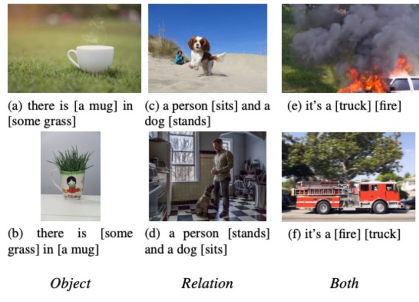
Figure 5: Example visualizations of Winoground swap types. Each category corresponds to a different type of linguistic swap in the caption. Object swaps noun phrases, Relation swaps verbs, adjectives, or adverbs, and Both can swap entities of both kinds.

Model	Object	Relation	Both	Average
Random Chance	25.0	25.0	25.0	25.0
CLIP ViT-L/14	27.0	25.8	57.7	28.2
OpenCLIP ViT-H/14	39.0	26.6	57.7	33.0
Diffusion Classifier (ours)	46.1	29.2	80.8	38.5

Table 3: Compositional reasoning results on Winoground. Diffusion Classifier obtains signficantly better text score (Eq. 9) than the contrastive baselines for all three swap categories.

Results

Table 3 compares Diffusion Classifier to two strong contrastive baselines: OpenCLIP ViT-H/14 (whose text embeddings Stable Diffusion conditions on) and CLIP ViT-L/14. Diffusion Classifier significantly outperforms both discriminative approaches on Winoground. Our method is stronger on all three swap types, even the challenging “Relation” swaps where the contrastive baselines do no better than random guessing. This indicates that Diffusion Classifier’s generative approach exhibits better compositional reasoning abilities. Since Stable Diffusion uses the same text encoder as OpenCLIP ViT-H/14, this improvement comes from better cross-modal binding of concepts to images. Overall, we find it surprising that Stable Diffusion, trained with only sample generation in mind, can be repurposed into such a strong classifier and reasoner without any additional training.

6.3 Supervised Classification Results

We compare Diffusion Classifier, leveraging the ImageNet-trained DiT-XL/2 model [58], to ViTs [22] and ResNets [29] trained on ImageNet. This setting is particularly interesting because it enables a fair comparison between models trained on the same dataset. Table 4 shows that Diffusion Classifier outperforms ResNet-101 and ViT-L/32. Diffusion Classifier achieves ImageNet accuracies of 77.5% and 79.1% at resolutions $256^{2}$ and $512^{2}$ respectively. To the best of our knowledge, we are the first to show that a generative model trained to learn $p_{\theta}(\mathbf{x}\mid\mathbf{c})$ can achieve ImageNet classification accuracy comparable to highly competitive discriminative methods.

Method ID OOD IN IN-V2 IN-A ObjectNet ResNet-18 70.3 57.3 1.1 27.2 ResNet-34 73.8 61.0 1.9 31.6 ResNet-50 76.7 63.2 0.0 36.4 ResNet-101 77.7 65.5 4.7 39.1 ViT-L/32 77.9 64.4 11.9 32.1 ViT-L/16 80.4 67.5 16.7 36.8 ViT-B/16 81.2 69.6 20.8 39.9 Diffusion Classifier $256^{2}$ 77.5 64.6 20.0 32.1 Diffusion Classifier $512^{2}$ 79.1 66.7 30.2 33.9

Table 4: Standard classification on ImageNet. We compare Diffusion Classifier (using DiT-XL/2 at $256^{2}$ and $512^{2}$ resolutions) to discriminative models trained on ImageNet. We highlight cells where Diffusion Classifier does better. All models (generative and discriminative) have only been trained on ImageNet.

6.3.1 Better Out-of-distribution Generalization

We find that Diffusion Classifier surprisingly has stronger out-of-distribution (OOD) performance on ImageNet-A than all of the baselines. In fact, our method shows qualitatively different and better OOD generalization behavior than discriminative approaches. Previous work [74] evaluated hundreds of discriminative models and found a tight linear relationship between their in-distribution (ID) and OOD accuracy — for a given ID accuracy, no models do better OOD than predicted by the linear relationship. For models trained on only ImageNet-1k (no extra data), none of a wide variety of approaches, from adversarial training to targeted augmentations to different architectures, achieve better OOD accuracy than predicted. We show the relationship between ID ImageNet accuracy (subsampled to the classes that overlap with ImageNet-A) and OOD accuracy on ImageNet-A for these discriminative models as the blue points (“standard training”) in Figure 6. The OOD accuracy is described well by a piecewise linear fit, with a kink at the ImageNet accuracy of the ResNet-50 model used to identify the hard images that comprise ImageNet-A. No discriminative models show meaningful “effective robustness,” which is the gap between the actual OOD accuracy of a model and the OOD accuracy predicted by the linear fit [74].

However, in contrast to these hundreds of discriminative models, Diffusion Classifier achieves much higher OOD accuracy on ImageNet-A than predicted. Figure 6 shows that Diffusion Classifier lies far above the linear fit and achieves an effective robustness of 15-25%. To the best of our knowledge, this is the first approach to achieve significant effective robustness without using any extra data during training.

There are a few caveats to our finding. Diffusion Classifier does not show improved effective robustness on the ImageNetV2 or ObjectNet distribution shifts, though perhaps the nature of those shifts is different from that of ImageNet-A. Diffusion Classifier may do better on ImageNet-A since its predictions could be less correlated with the (discriminative) ResNet-50 used to find hard examples for ImageNet-A. Nevertheless, the dramatic improvement in effective robustness on ImageNet-A is exciting and suggests that generative classifiers are promising approaches to achieve better robustness to distribution shift.

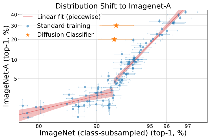
Figure 6: Diffusion Classifier exhibits effective robustness without using extra labeled data. Compared to discriminative models trained on the same amount of labeled data (“standard training”), Diffusion Classifier achieves much higher ImageNet-A accuracy than predicted by its ImageNet accuracy. Diffusion Classifier points correspond to DiT-XL/2 at resolution $256^{2}$ and $512^{2}$. Points are shown with 99.5% Clopper-Pearson confidence intervals. The red lines show the linear relationship between ID and OOD accuracy for discriminative models, with a “break” at the accuracy of the model used to create ImageNet-A. The axes were adjusted using logit scaling, since accuracies fall within $[0,100]$.

6.3.2 Stable Training and No Overfitting

Diffusion Classifier’s ImageNet accuracy is especially impressive since DiT was trained with only random horizontal flips, unlike typical classifiers that use RandomResizedCrop, Mixup [82], RandAugment [14], and other tricks to avoid overfitting. Training DiT with more advanced augmentations should further improve its accuracy. Furthermore, DiT training is stable with fixed learning rate and no regularization other than weight decay [58]. This stands in stark contrast with ViT training, which is unstable and frequently suffers from NaNs, especially for large models [28]. These results indicate that the generative objective $\log p_{\theta}(\mathbf{x}\mid\mathbf{c})$ could be a promising way to scale up training to even larger models without overfitting or instability.

6.3.3 Choice of classification objective

While Stable Diffusion parameterizes $p_{\theta}(\mathbf{x}_{t-1}\mid\mathbf{x}_{t},\mathbf{c})$ as a Gaussian with fixed variance, DiT learns the variance $\Sigma_{\theta}(\mathbf{x_{t}},\mathbf{c})$. A single network outputs $\epsilon_{\theta}$ and $\Sigma_{\theta}$, but they are trained via two separate losses. $\epsilon_{\theta}$ is trained via a uniform weighting of $\ell_{2}$ errors $\mathbb{E}_{\epsilon,t}[\|\epsilon-\epsilon_{\theta}(\mathbf{x}_{t},\mathbf{c})\|^{2}]$, as this is found to improve sample quality. In contrast, $\Sigma_{\theta}$ is trained with the exact variational lower bound. This keeps the timestep-dependent weighting term $w_{t}$ in Eq. 3 and weights the $\epsilon$-prediction errors by the inverse of the variances $\Sigma_{\theta}$ (see [58] for more details). Since both losses are used at training time, we run an experiment to see which objective yields the best accuracy as an inference-time objective. Instead of choosing the class with the lowest error based on uniform $\ell_{2}$ weighting, as is done in Algorithm 1, we additionally try using the variational bound or the sum of the uniform weighting and the variational bound. Table 5 shows that the uniform $\ell_{2}$ weighting does best across all datasets. This justifies the approximation we made to the ELBO in Eq. 4. The sum of the uniform $\ell_{2}$ and the variational bound does almost as well, likely because the magnitude of the variational bound is much smaller than that of the uniformly weighted $\ell_{2}$, so their sum is dominated by the $\ell_{2}$ term.

Resolution Objective IN IN-v2 IN-A ObjectNet $\ell_{2}$ 77.5 64.6 20.0 33.9 $256^{2}$ VLB 71.6 57.7 17.9 24.7 $\ell_{2}$ + VLB 77.5 64.6 20.0 33.8 $\ell_{2}$ 79.1 66.7 30.2 33.9 $512^{2}$ VLB 74.0 59.1 24.9 24.7 $\ell_{2}$ + VLB 79.0 66.6 30.2 33.8

Table 5: Effect of classification objective. DiT trains $\epsilon_{\theta}$ with the uniformly weighted $\ell_{2}$ loss to evaluate $\sum_{t}w_{t}\|\epsilon-\epsilon_{\theta}(\mathbf{x}_{t},\mathbf{c})\|^{2}$ from Eq. 3. DiT also trains the learned variance $\Sigma_{\theta}$ of $p_{\theta}(\mathbf{x}_{t-1}|\mathbf{x}_{t})$ with the exact variational lower bound, which weights timesteps unevenly. Since both of these weightings are involved in DiT training, we try each objective, as well as their sum, to see which one achieves the best accuracy. We find that uniformly weighting $\ell_{2}$ errors across timesteps performs best.

7 Conclusion and Discussion

We investigated the zero-shot and standard classification abilities of diffusion models by leveraging them as conditional density estimators. By performing a simple, unbiased Monte Carlo estimate of the learned conditional ELBO for each class, we extract Diffusion Classifier—a powerful approach to turn any conditional diffusion model into a classifier without any additional training. We find that this classifier narrows the gap with state-of-the-art discriminative approaches on zero-shot and standard classification and significantly outperforms them on multimodal compositional reasoning. Diffusion Classifier also exhibits far better “effective robustness” to distribution shift.

Accelerating Inference

While inference time is currently a practical bottleneck, there are several clear ways to accelerate Diffusion Classifier. Decreasing resolution from the default $512\times 512$ (for SD) would yield a dramatic speedup. Inference at $256\times 256$ is at least $4\times$ faster, and inference at $128\times 128$ would be over $16\times$ faster. Another option is to use a weak discriminative model to quickly eliminate classes that are clearly incorrect. Appendix B shows that this would simultaneously improve accuracy and reduce inference time. Gradient-based search could backpropagate through the diffusion model to solve $\operatorname*{arg\,max}_{c}\log p(x\mid c)$, which could eliminate the runtime dependency on the number of classes. New architectures could be designed to only use the class conditioning $c$ toward the end of the network, enabling reuse of intermediate activations across classes. Finally, note that the error prediction process is easily parallelizable. With sufficient scaling or better GPUs in the future, all Diffusion Classifier steps can be done in parallel with the latency of a single forward pass.

Role of Diffusion Model Design Decisions

Since we don’t change the base diffusion model of Diffusion Classifier, the choices made during diffusion training affect the classifier. For instance, Stable Diffusion [65] conditions the image generation on the text embeddings from OpenCLIP [38]. However, the language model in OpenCLIP is much weaker than open-ended large-language models like T5-XXL [62] because it is only trained on text data available from image-caption pairs, a minuscule subset of total text data on the Internet. Hence, we believe that diffusion models trained on top of T5-XXL embeddings, such as Imagen [67], should display better zero-shot classification results, but these are not open-source to empirically validate. Other design choices, such as whether to perform diffusion in latent space (e.g. Stable Diffusion) or in pixel space (e.g. DALLE 2), can also affect the adversarial robustness of the classifier and present interesting avenues for future work.

In conclusion, while generative models have previously fallen short of discriminative ones for classification, today’s pace of advances in generative modeling means that they are rapidly catching up. Our strong classification, multimodal compositional reasoning, and robustness results represent an encouraging step in this direction.

Acknowledgements We thank Patrick Chao for helpful discussions and Christina Baek and Rishi Veerapaneni for paper feedback. Stability.AI contributed compute to run some experiments. AL is supported by the NSF GRFP DGE1745016 and DGE2140739. This work is supported by NSF IIS-2024594 and ONR MURI N00014-22-1-2773.

Appendix

Appendix A Efficient Diffusion Classifier Algorithm

Though Diffusion Classifier works straightforwardly with the procedure described in Algorithm 1, we are interested in speeding up inference as described in Section 4.2. Algorithm 2 shows the efficient Diffusion Classifier procedure that adaptively chooses which classes to continue evaluating. Table 6 shows the evaluation strategy used for each zero-shot dataset. We hand-picked the strategies based on the number of classes in each dataset. Further gains in accuracy may be possible with more evaluations.

Algorithm 2 Diffusion Classifier (Adaptive)

1:  Input: test image $\mathbf{x}$, conditioning inputs $\mathcal{C}=\{\mathbf{c}_{i}\}_{i=1}^{n}$ (e.g., text embeddings or class indices), number of stages $N_{\text{stages}}$, list KeepList of number of $\mathbf{c}_{i}$ to keep after each stage, list TrialList of number of trials done by each stage

2:  Initialize $\texttt{Errors}[\mathbf{c}_{i}]=\text{list}()$ for each $\mathbf{c}_{i}$

3:  Initialize PrevTrials = 0    // How many times we’ve tried each remaining element of $\mathcal{C}$ so far

4:  for stage i $=1,\dots,N_{\text{stages}}$ do

5:     for trial $j=1,\dots,\texttt{TrialList}[i]-\texttt{PrevTrials}$ do

6:        Sample $t\sim[1,1000]$

7:        Sample $\epsilon\sim\mathcal{N}(0,I)$

8:        $\mathbf{x}_{t}=\sqrt{\bar{\alpha}_{t}}\mathbf{x}+\sqrt{1-\bar{\alpha}_{t}}\epsilon$

9:        for conditioning $\mathbf{c}_{k}\in\mathcal{C}$ do

10:           $\texttt{Errors}[\mathbf{c}_{k}].\texttt{append}(\|\epsilon-\epsilon_{\theta}(\mathbf{x}_{t},\mathbf{c}_{k})\|^{2})$

11:        end for

12:     end for

13:     $\displaystyle\mathcal{C}\leftarrow\operatorname*{arg\,min}_{\begin{subarray}{c}\mathcal{S}\subset\mathcal{C};\\ |\mathcal{S}|=\texttt{KeepList}[i]\end{subarray}}\sum_{c_{k}\in\mathcal{S}}\texttt{mean}(\texttt{Errors}[\mathbf{c}_{k}])$    // Keep top $\texttt{KeepList}[i]$ conditionings $\mathbf{c}_{k}$ with the lowest errors

14:     PrevTrials = TrialList[i]

15:  end for

16:  return  $\displaystyle\operatorname*{arg\,min}_{\mathbf{c}_{i}\in\mathcal{C}}\texttt{\,mean}(\texttt{Errors}[\mathbf{c}_{i}])$

Dataset	Prompts kept per stage	Evaluations per stage	Avg. evaluations per class	Total evaluations
Food101	20 10 5 1	20 50 100 500	50.7	5120
CIFAR10	5 1	50 500	275	2750
Aircraft	20 10 5 1	20 50 100 500	51	5100
Pets	5 1	25 250	51	1890
Flowers102	20 10 5 1	20 50 100 500	50.4	5140
STL10	5 1	100 500	300	3000
ImageNet	500 50 10 1	50 100 500 1000	100	100000
ObjectNet	25 10 5 1	50 100 500 1000	118.6	13400

Table 6: Adaptive evaluation strategy for each zero-shot dataset.

Appendix B Inference Costs and Hybrid Classification Approach

Food101 CIFAR10 Aircraft Oxford Pets Flowers102 STL10 ImageNet Diffusion Classifier 77.7 88.5 26.4 87.3 66.3 95.4 61.4 Time/img (s) 51 30 51 18 51 30 1000 Diffusion Classifier w/ discriminative pruning 78.7 88.5 26.8 86.4 67.0 95.4 62.6 Time/img (s) 35 30 35 18 35 30 150 Est. Time/img (s) at $128^{2}$ res 2 2 2 1 2 2 9 CLIP ResNet-50 81.1 75.6 19.3 85.4 65.9 94.3 58.2

Table 7: Zero-shot accuracy and inference time with Stable Diffusion $512\times 512$. “Pruning” away unlikely classes with a weak discriminative classifier (e.g., CLIP ResNet-50) increases accuracy and reduces inference time. Additionally, reducing resolution to $128\times 128$ would reduce inference time by roughly $16\times$. However, its impact on accuracy is difficult to estimate without retraining the Stable Diffusion model to expect lower resolutions. All times are estimated using a RTX 3090 GPU.

Table 7 shows the inference time of Diffusion Classifier when using the efficient Diffusion Classifier algorithm (Algorithm 2). Classifying a single image takes anywhere between 18 seconds (Pets) to 1000 seconds (ImageNet). The issue with ImageNet is that Diffusion Classifier inference time still approximately scales linearly with the number of classes, even when using the adaptive strategy. One way to address this problem is to use a weak discriminative model to quickly “prune” away classes that are almost certainly incorrect. Table 7 shows that using Diffusion Classifier to choose among the top 20 class predictions made by CLIP ResNet-50 for an image greatly reduces inference time, while even improving performance. This pruning procedure only requires the top-20 accuracy of the fast discriminative model to be high (close to 100%), so it works even when the top-1 accuracy of the ResNet-50 is low, like on Aircraft. We chose top-20 intuitively, without any hyperparameter search, and tuning the $k$ for top-$k$ pruning will trade off between inference time and accuracy. Note that no other results in this paper use the discriminative pruning procedure, to avoid conflating the capabilities of Diffusion Classifier with those of the weak discriminative model used to prune.

Appendix C Inference Objective Function

Food101 CIFAR10 Aircraft Oxford Pets Flowers102 STL10 ImageNet ObjectNet Squared $\ell_{2}$ 77.7 84.4 26.4 86.3 62.2 95.4 61.4 43.4 $\ell_{1}$ 73.8 88.4 22.1 87.3 66.3 95.4 59.6 36.8 Huber 77.7 84.6 26.7 86.6 62.6 95.4 60.9 43.5

Table 8: Diffusion Classifier zero-shot performance with different loss functions $\mathcal{L}(\epsilon-\epsilon_{\theta}(\mathbf{x}_{t},\mathbf{c}))$.

Resolution	Objective	ImageNet	ImageNetV2	ImageNet-A	ObjectNet
$256^{2}$	Squared $\ell_{2}$	77.5	64.6	20.0	32.1
$256^{2}$	$\ell_{1}$	74.9	60.5	9.7	24.7
$512^{2}$	Squared $\ell_{2}$	79.1	66.7	30.2	33.9
$512^{2}$	$\ell_{1}$	75.6	62.1	13.2	26.2

Table 9: Diffusion Classifier supervised performance with different loss functions $\mathcal{L}(\epsilon-\epsilon_{\theta}(\mathbf{x}_{t},\mathbf{c}))$.

While the theory in Section 3 justifies using $\|\epsilon-\epsilon_{\theta}(\mathbf{x}_{t},\mathbf{c})\|_{2}^{2}$ within the Diffusion Classifier inference objective, we surprisingly find that other loss functions can work better in some cases. Table 8 shows that $\|\epsilon-\epsilon_{\theta}(\mathbf{x}_{t},\mathbf{c})\|_{1}$ (the $\ell_{1}$ loss) instead of the squared $\ell_{2}$ loss does better on roughly half of the datasets that we use to evaluate the Stable Diffusion-based zero-shot classifier. This is puzzling, since the $\ell_{1}$ loss is neither theoretically justified nor appears in the Stable Diffusion training objective. We hope followup work can explain the empirical success of the $\ell_{1}$ loss. Combining these two losses does not get the “best of both worlds.” The Huber loss, which is the squared $\ell_{2}$ loss for values less than 1 and is the $\ell_{1}$ loss for values greater than 1, roughly achieves the same performance as the theoretically-justified squared $\ell_{2}$ loss. We choose between squared $\ell_{2}$ and $\ell_{1}$ as a hyperparameter for Section 6.1. Table 9 shows that $\ell_{1}$ does not help with supervised classification (Section 6.3) using DiT-XL/2.

Appendix D Interpretability via Image Generation

In contrast to discriminative classifiers, where it is difficult to understand what features the model has learned or why a model has made a certain decision, generative classifiers are easier to visualize. In this section, we examine how samples from the generative model can help us understand class-dependent features that the model has learned as well as failures in the model’s understanding.

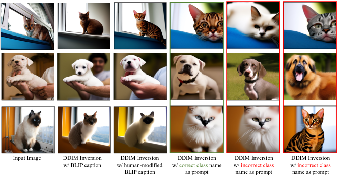
Figure 7: Analyzing Diffusion Classifier for Zero-Shot Classification: We analyze the role of different text/captions (BLIP, Human-modified BLIP, correct class-name, incorrect class-name) for zero-shot classification using text-based diffusion models. To do so, we invert the input image using the corresponding caption and then reconstruct it using deterministic DDIM sampling. The image inverted and reconstructed using a human-modified BLIP caption aligns the most with the input image since this caption is the most descriptive. The images reconstructed using correct class names as prompts (column 4) align much better with the input image in terms of class-descriptive features of the underlying object than the images reconstructed using incorrect class names as prompts (columns 5 and 6). Row 3 (columns 4 and 5) demonstrates an example where the base Stable Diffusion does not understand the difference between the two cat breeds, Birman and Ragdoll, and hence cannot invert/sample them differently. As a result, our classifier also fails.

Experiment Setup

Given an input image, we first perform DDIM inversion [71, 41] (with 50 timesteps) using Stable Diffusion 2.0 and different captions as prompts: BLIP [48] generated caption, human-refined BLIP generated caption, “a photo of {correct-class-name}, a type of pet” and “a photo of {incorrect-class-name}, a type of pet.”. Next, we leverage the inverted DDIM latent and the corresponding prompt to attempt to reconstruct the original image (using a deterministic diffusion scheduler [71]). The underlying intuition behind this experiment is that the inverted image should look more similar to the original image when a correct and appropriate/descriptive prompt is used for DDIM inversion and sampling.

Experimental Evaluation

Figure 7 shows the results of this experiment for the Oxford-IIIT Pets dataset. The image inverted using a human-modified BLIP caption (column 3) is the most similar to the original image (column 1). This aligns with our intuition as this caption is most descriptive of the input image. The human-modified caption only adds the correct class name (Bengal Cat, American Bull Dog, Birman Cat) ahead of the BLIP predicted “cat or dog” token for the foreground object and slightly enhances the description for the background. Comparing the BLIP-caption results (column 2) with the human-modified BLIP-caption results (column 3), we can see that by just using the class-name as the extra token, the diffusion model can inherit class-descriptive features. The Bengal cat has stripes, the American Bulldog has a wider chin, and the Birman cat has a black patch on its face in the reconstructed image.

Compared to the images generated using the human-generated caption as a prompt, the images reconstructed using only class names as prompts (columns 4,5,6) align less with the input image (column 1). This is expected, as class names by themselves are not dense descriptions of the input images. Comparing the results of column 4 (correct class names as prompt) with those of column 5,6 (incorrect class names as prompt), we can see that the foreground object has similar class-descriptive features (brown and black stripes in row 1 and black face patches in row 3) to the input image for the correct-prompt reconstructions. This highlights the fact that although using class names as approximate prompts will not lead to perfect denoising (Eq. 7), for the global prediction task of classification, the correct class names should provide enough descriptive features for denoising, relative to the incorrect class names.

Row 3 of Figure 7 further highlights an example of a failure mode where Stable Diffusion generates very similar inverted images for correct Birman and incorrect Ragdoll text prompts. As a result, our model also incorrectly classifies the Birman cat as a Ragdoll. To fix this failure mode, we tried finetuning the Stable Diffusion model on a dataset of Ragdoll/Birman cats (175 images in total). Using this finetuned model, Diffusion Classifier accuracy on these two classes increases to 85%, from an initial zero-shot accuracy of 45%. In addition to minimizing the standard $\epsilon$-prediction error $\|\epsilon-\epsilon_{\theta}(\mathbf{x}_{t},\mathbf{c}_{i})\|^{2}$, we found that adding a loss term to increase the error $\|\epsilon-\epsilon_{\theta}(\mathbf{x}_{t},\mathbf{c}_{j})\|^{2}$ for the wrong class $\mathbf{c}_{j}$ helped the model distinguish these commonly-confused classes.

Appendix E How Does Stable Diffusion Version Affect Zero-Shot Accuracy?

SD Version Food101 CIFAR10 Aircraft Oxford Pets Flowers102 STL10 ImageNet ObjectNet 1.1 60.3 83.4 20.1 78.8 43.1 92.6 51.7 38.1 1.2 75.7 85.9 26.3 85.4 54.4 94.4 57.3 39.4 1.3 77.5 87.5 27.8 87.2 54.5 94.9 59.7 40.9 1.4 77.8 86.0 28.6 87.4 54.2 94.8 59.2 41.2 1.5 78.4 85.5 29.1 87.5 55.0 94.5 59.6 41.6 2.0 77.7 88.5 26.4 87.3 66.3 95.4 61.4 43.4 2.1 77.9 87.1 24.3 86.2 59.4 95.3 58.4 38.3

Table 10: Effect of Stable Diffusion version on Diffusion Classifier zero-shot accuracy. We bold the best version within SD 1.x and 2.x. For SD 1, accuracy tends to increase with more training. The main exception is on low-resolution datasets like CIFAR10 and STL10. SD 2 performance consistently decreases from SD 2.0 to SD 2.1 on almost every dataset.

We investigate how much the Stable Diffusion checkpoint version affects Diffusion Classifier’s zero-shot classification accuracy. Table 10 shows zero-shot accuracy for each Stable Diffusion release version so far. We use the same adaptive evaluation strategy (Algorithm 2) for each version. Accuracy improves with each new release for SD 1.x, as more training likely reduces underfitting on the training data. However, accuracy actually decreases when going from SD 2.0 to 2.1. The cause of this is not clear, especially without access to intermediate training checkpoints. One hypothesis is that further training on $512^{2}$ resolution images causes the model to forget knowledge from its initial $256^{2}$ resolution training set, which is closer to the distribution of these zero-shot benchmarks. SD 2.1 was finetuned using a more permissive NSFW threshold ($\geq 0.98$ instead of $\geq 0.1$), so another hypothesis is that this introduced a lot of human images that hurt performance on our object-centric benchmarks.

Appendix F Additional Implementation Details

F.1 Zero-shot classification using Diffusion Classifier

Training Data

For our zero-shot Diffusion Classifier, we utilize Stable Diffusion 2.0 [65]. This model was trained on a subset of the LAION-5B dataset, filtered so that the training data is aesthetic and appropriately safe-for-work. LAION classifiers were used to remove samples that are too small (less than $512\times 512$), potentially not-safe-for-work (punsafe $\geq 0.1$), or unaesthetic (aesthetic score $\leq 4.5$). These thresholds are conservative, since false negatives (NSFW or undesirable images left in the training set) are worse than removing extra images from a large starting dataset. As discussed in Section 6.1, these filtering criteria bias the distribution of Stable Diffusion training data and likely negatively affect Diffusion Classifier’s performance on datasets whose images do not satisfy these criteria. SD 2.0 was trained for 550k steps at resolution $256\times 256$ on this subset, followed by an additional 850k steps at resolution $512\times 512$ on images that are at least that large. This checkpoint can be downloaded online through the diffusers repository at stabilityai/stable-diffusion-2-0-base.

Inference Details

We use FP16 and Flash Attention [15] to improve inference speed. This enables efficient inference with a batch size of 32, which works across a variety of GPUs, from RTX 2080Ti to A6000. We found that adding these two tricks did not affect test accuracy compared to using FP32 without Flash Attention. Given a test image, we resize the shortest edge to 512 pixels using bicubic interpolation, take a $512\times 512$ center crop, and normalize the pixel values to $[-1,1]$. We then use the Stable Diffusion autoencoder to encode the $512\times 512\times 3$ RGB image into a $64\times 64\times 4$ latent. We finally classify the test image by applying the method described in Sections 3 and 4 to estimate $\epsilon$-prediction error in this latent space.

F.2 Compositional reasoning using Diffusion Classifier

For our experiments on the Winoground benchmark [75], most details are the same as the zero-shot details described in Appendix F.1. We use Stable Diffusion 2.0, and we evaluate each image-caption pair with 1000 evenly spaced timesteps. We omit the adaptive inference strategy since there are only 4 image-caption pairs to evaluate for each Winoground example.

F.3 ImageNet classification using Diffusion Classifier

For this task, we use the recently proposed Diffusion Transformer (DiT) [58] as the backbone of our Diffusion Classifier. DiT was trained on ImageNet-1k, which contains about 1.28 million images from 1,000 classes. While it was originally trained to produce high-quality samples with strong FID scores, we repurpose the model and compare it against discriminative models with the same ImageNet-1k training data. We use the DiT-XL/2 model size at resolution $256^{2}$ and $512^{2}$. Notably, DiT achieves strong performance while using much weaker data augmentations than what discriminative models are usually trained with. During training time for the $256^{2}$ checkpoint, the smaller edge of the input image is resized to 256 pixels. Then, a $256\times 256$ center crop is taken, followed by a random horizontal flip, followed by embedding with the Stable Diffusion autoencoder. A similar process is done for the $512^{2}$ model. At test time, we follow the same preprocessing pipeline, but omit the random horizontal flip. Classification performance could improve if stronger augmentations, like RandomResizedCrop or color jitter, are used during the diffusion model training process.

F.4 Baselines for Zero-Shot Classification

Synthetic SD Data:

We provide the implementation details of the “Synthetic SD Data” baseline (row 1 of Table 1) for the task of zero-shot image classification. Our Diffusion Classifier approach builds on the intuition that a model capable of generating examples of desired classes should be able to directly discriminate between them. In contrast, this baseline takes the simple approach of using our generative model, Stable Diffusion, as intended to generate synthetic training data for a discriminative model. For a given dataset, we use pre-trained Stable Diffusion 2.0 with default settings to generate $10{,}000$ synthetic $512\times 512$ pixel images per class as follows: we use the English class name and randomly sample a template from those provided by the CLIP [60] authors to form the prompt for each generation. We then train a supervised ResNet-50 classifier using the synthetic data and the labels corresponding to the class name that was used to generate each image. We use batch size $=256$, weight decay $=1e-4$, learning rate $=0.1$ with a cosine schedule, the AdamW optimizer, and use random resized crop & horizontal flip transforms. We create a validation set using the synthetic data by randomly selecting 10% of the images for each class; we use this for early stopping to prevent over-fitting. Finally, we report the accuracy on the target dataset’s proper test set.

SD Features:

We provide the implementation details of the “SD Features” baseline (row 2 of Table 1) for the task of image classification. This baseline is inspired by Label-DDPM [3], a recent work on diffusion-based semantic segmentation. Unlike Label-DDPM, which leverages a category-specific diffusion model, we directly build on top of the open-sourced Stable Diffusion model (trained on the LAION dataset). We then approach the task of classification as follows: given the pre-trained Stable Diffusion model, we extract the intermediate U-Net features corresponding to the input image. These features are then passed through a ResNet-based classifier to predict logits for the potential classes. To extract the intermediate U-Net features, we add a noise equivalent to the $100th$ timestep noise to the input image and evaluate the corresponding noisy latent using the forward diffusion process. We then pass the noisy latent through the U-Net model, conditioned on timestep $t=100$ and text conditioning ($\mathbf{c}$) as an empty string, and extract the features from the mid-layer of the U-Net at a resolution of [8 × 8 × 1024]. Next, we train a supervised classifier on top of these features. Thus, this baseline is not zero-shot. The architecture of our classifier is similar to ResNet-18, with small modifications to make it compatible with an input size of $[8\times 8\times 1024]$. Table 11 defines these modifications. We set batch size $=16$, learning rate $=1e-4$, and use the AdamW optimizer. During training, we apply image augmentations typically used by discriminative classifiers (RandomResizedCrop and horizontal flip). We do early stopping using the validation set to prevent overfitting.

Arch	Conv1	Conv2	Conv3 x2	Conv4 x2	Conv5 x2
ResNet-18	7x7x64	3x3 max-pool	3x3x128	3x3x256	3x3x512
ResNet-18 (SD Features)	3x3x1280	-	3x3x1280	3x3x2560	3x3x2560

Table 11: Comparison of SD Features’ ResNet-18 classifier architecture with the original ResNet-18

Appendix G Techniques that did not help

Diffusion Classifier requires many samples to accurately estimate the ELBO. In addition to using the techniques in Section 3 and 4, we tried several other options for variance reduction. None of the following methods worked, however. We list negative results here for completeness, so others do not have to retry them.

Classifier-free guidance

Classifier-free guidance [36] is a technique that improves the match between a prompt and generated image, at the cost of mode coverage. This is done by training a conditional $\epsilon_{\theta}(\mathbf{x}_{t},\mathbf{c})$ and unconditional $\epsilon_{\theta}(\mathbf{x}_{t})$ denoising network and combining their predictions at sampling time:

$$\tilde{\epsilon}(\mathbf{x}_{t},\mathbf{c})=(1+w)\epsilon_{\theta}(\mathbf{x}_{t},\mathbf{c})-w\epsilon_{\theta}(\mathbf{x}_{t})$$ (10)

where $w$ is a guidance weight that is typically in the range $[0,10]$. Most diffusion models are trained to enable this trick by occasionally replacing the conditioning $\mathbf{c}$ with an empty token. Intuitively, classifier-free guidance “sharpens” $\log p_{\theta}(x\mid\mathbf{c})$ by encouraging the model to move away from regions that unconditionally have high probability. We test Diffusion Classifier to see if using the $\tilde{\epsilon}$ from classifier-free guidance can improve confidence and classification accuracy. Our new $\epsilon$-prediction metric is now $\left\|\epsilon-(1+w)\epsilon_{\theta}(\mathbf{x}_{t},\mathbf{c})-w\epsilon_{\theta}(\mathbf{x}_{t})\right\|^{2}$. However, Figure 9 shows that $w=0$ (i.e., no classifier-free guidance) performs best. We hypothesize that this is because Diffusion Classifier fails on uncertain examples, which classifier-free guidance affects unpredictably.

Error map cropping

The ELBO $\mathbb{E}_{t,\epsilon}[\|\epsilon-\epsilon_{\theta}(\mathbf{x}_{t},\mathbf{c})\|^{2}]$ depends on accurately estimating the added noise at every location of the $64\times 64\times 4$ image latent. We try to reduce the impact of edge pixels (which are less likely to contain the subject) by computing $\mathbf{x}_{t}$ as normal, but only measuring the ELBO on a center crop of $\epsilon$ and $\epsilon_{\theta}(\mathbf{x}_{t},\mathbf{c})$. We compute:

$$\|\epsilon_{[i:-i,i:-i]}-\epsilon_{\theta}(\mathbf{x}_{t},\mathbf{c})_{[i:-i,i:-i]}\|^{2}$$ (11)

where $i$ is the number of latent “pixels” to remove from each edge. However, Figure 9 shows that any amount of cropping reduces accuracy.

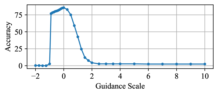
Figure 8: Accuracy plot of classifier-free guidance on Pets.

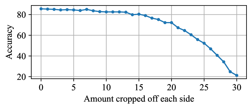
Figure 9: Cropping $\epsilon$ and $\epsilon_{\theta}(\mathbf{x}_{t},\mathbf{c})$ reduces accuracy on Pets.

Importance sampling

Importance sampling is a common method for reducing the variance of a Monte Carlo estimate. Instead of sampling $\epsilon\sim\mathcal{N}(0,I)$, we sample $\epsilon$ from a narrower distribution. We first tried fixing $\epsilon=0$, which is the mode of $\mathcal{N}(0,I)$, and only varying the timestep $t$. We also tried the truncation trick [7] which samples $\epsilon\sim\mathcal{N}(0,I)$ but continually resamples elements that fall outside the interval $[a,b]$. Finally, we tried sampling $\epsilon\sim\mathcal{N}(0,I)$ and rescaling them to the expected norm ($\epsilon\rightarrow\frac{\epsilon}{\|\epsilon\|_{2}}\mathbb{E}_{\epsilon^{\prime}}[\|\epsilon^{\prime}\|_{2}])$) so that there are no outliers. Table 12 shows that none of these importance sampling strategies improve accuracy. This is likely because the noise $\epsilon$ sampled with these strategies are completely out-of-distribution for the noise prediction model. For computational reasons, we performed this experiment on a 10% subset of Pets.

Sampling distribution for $\epsilon$	Pets accuracy
$\epsilon=0$	41.3
TruncatedNormal, $[-1,1]$	49.9
TruncatedNormal, $[-2.5,2.5]$	81.5
Expected norm	86.9
$\epsilon\sim\mathcal{N}(0,I)$	87.5

Table 12: Every importance sampling strategy underperforms sampling the noise $\epsilon$ from a standard normal distribution.

References

- [1] Jean-Baptiste Alayrac, Jeff Donahue, Pauline Luc, Antoine Miech, Iain Barr, Yana Hasson, Karel Lenc, Arthur Mensch, Katherine Millican, Malcolm Reynolds, et al. Flamingo: a visual language model for few-shot learning. Advances in Neural Information Processing Systems, 35:23716–23736, 2022.
- [2] Peter Auer. Using confidence bounds for exploitation-exploration trade-offs. Journal of Machine Learning Research, 3(Nov):397–422, 2002.
- [3] Dmitry Baranchuk, Andrey Voynov, Ivan Rubachev, Valentin Khrulkov, and Artem Babenko. Label-efficient semantic segmentation with diffusion models. In International Conference on Learning Representations, 2022.
- [4] Andrei Barbu, David Mayo, Julian Alverio, William Luo, Christopher Wang, Dan Gutfreund, Joshua B. Tenenbaum, and Boris Katz. Objectnet: A large-scale bias-controlled dataset for pushing the limits of object recognition models. In Neural Information Processing Systems, 2019.
- [5] David M. Blei, Alp Kucukelbir, and Jon D. McAuliffe. Variational inference: A review for statisticians. Journal of the American Statistical Association, 2017.
- [6] Lukas Bossard, Matthieu Guillaumin, and Luc Van Gool. Food-101 – mining discriminative components with random forests. In European Conference on Computer Vision, 2014.
- [7] Andrew Brock, Jeff Donahue, and Karen Simonyan. Large scale gan training for high fidelity natural image synthesis. arXiv preprint arXiv:1809.11096, 2018.
- [8] Tom Brown, Benjamin Mann, Nick Ryder, Melanie Subbiah, Jared D Kaplan, Prafulla Dhariwal, Arvind Neelakantan, Pranav Shyam, Girish Sastry, Amanda Askell, et al. Language models are few-shot learners. Advances in neural information processing systems, 33:1877–1901, 2020.
- [9] Ryan Burgert, Kanchana Ranasinghe, Xiang Li, and Michael S Ryoo. Peekaboo: Text to image diffusion models are zero-shot segmentors. arXiv preprint arXiv:2211.13224, 2022.
- [10] Xi Chen, Yan Duan, Rein Houthooft, John Schulman, Ilya Sutskever, and Pieter Abbeel. Infogan: Interpretable representation learning by information maximizing generative adversarial nets. Advances in neural information processing systems, 29, 2016.
- [11] Mehdi Cherti, Romain Beaumont, Ross Wightman, Mitchell Wortsman, Gabriel Ilharco, Cade Gordon, Christoph Schuhmann, Ludwig Schmidt, and Jenia Jitsev. Reproducible scaling laws for contrastive language-image learning. arXiv preprint arXiv:2212.07143, 2022.
- [12] Adam Coates, Andrew Ng, and Honglak Lee. An analysis of single-layer networks in unsupervised feature learning. In Geoffrey Gordon, David Dunson, and Miroslav Dudík, editors, Proceedings of the Fourteenth International Conference on Artificial Intelligence and Statistics, volume 15 of Proceedings of Machine Learning Research, pages 215–223, Fort Lauderdale, FL, USA, 11–13 Apr 2011. PMLR.
- [13] Danilo Croce, Giuseppe Castellucci, and Roberto Basili. GAN-BERT: Generative adversarial learning for robust text classification with a bunch of labeled examples. In Proceedings of the 58th Annual Meeting of the Association for Computational Linguistics, 2020.
- [14] Ekin D Cubuk, Barret Zoph, Jonathon Shlens, and Quoc V Le. Randaugment: Practical automated data augmentation with a reduced search space. In Proceedings of the IEEE/CVF conference on computer vision and pattern recognition workshops, pages 702–703, 2020.
- [15] Tri Dao, Daniel Y. Fu, Stefano Ermon, Atri Rudra, and Christopher Ré. FlashAttention: Fast and memory-efficient exact attention with IO-awareness. In Advances in Neural Information Processing Systems, 2022.
- [16] Mostafa Dehghani, Josip Djolonga, Basil Mustafa, Piotr Padlewski, Jonathan Heek, Justin Gilmer, Andreas Steiner, Mathilde Caron, Robert Geirhos, Ibrahim Alabdulmohsin, et al. Scaling vision transformers to 22 billion parameters. arXiv preprint arXiv:2302.05442, 2023.
- [17] Jia Deng, Wei Dong, Richard Socher, Li-Jia Li, Kai Li, and Li Fei-Fei. Imagenet: A large-scale hierarchical image database. In 2009 IEEE conference on computer vision and pattern recognition, pages 248–255. Ieee, 2009.
- [18] Jacob Devlin, Ming-Wei Chang, Kenton Lee, and Kristina Toutanova. Bert: Pre-training of deep bidirectional transformers for language understanding. preprint arXiv:1810.04805, 2018.
- [19] Jacob Devlin, Ming-Wei Chang, Kenton Lee, and Kristina Toutanova. Bert: Pre-training of deep bidirectional transformers for language understanding. ArXiv, abs/1810.04805, 2019.
- [20] Prafulla Dhariwal and Alexander Nichol. Diffusion models beat gans on image synthesis. NeurIPS, 2021.
- [21] Laurent Dinh, Jascha Sohl-Dickstein, and Samy Bengio. Density estimation using real nvp. CoRR, abs/1605.08803, 2016.
- [22] Alexey Dosovitskiy, Lucas Beyer, Alexander Kolesnikov, Dirk Weissenborn, Xiaohua Zhai, Thomas Unterthiner, Mostafa Dehghani, Matthias Minderer, Georg Heigold, Sylvain Gelly, et al. An image is worth 16x16 words: Transformers for image recognition at scale. preprint arXiv:2010.11929, 2020.
- [23] Yilun Du and Igor Mordatch. Implicit generation and generalization in energy-based models. ArXiv, abs/1903.08689, 2019.
- [24] Aditya Ramesh et al. Hierarchical text-conditional image generation with clip latents, 2022.
- [25] Samir Yitzhak Gadre, Mitchell Wortsman, Gabriel Ilharco, Ludwig Schmidt, and Shuran Song. Clip on wheels: Zero-shot object navigation as object localization and exploration. arXiv preprint arXiv:2203.10421, 2022.
- [26] Ian Goodfellow, Jean Pouget-Abadie, Mehdi Mirza, Bing Xu, David Warde-Farley, Sherjil Ozair, Aaron Courville, and Yoshua Bengio. Generative adversarial nets. In Advances in neural information processing systems, pages 2672–2680, 2014.
- [27] Will Grathwohl, Kuan-Chieh Wang, Joern-Henrik Jacobsen, David Duvenaud, Mohammad Norouzi, and Kevin Swersky. Your classifier is secretly an energy based model and you should treat it like one. In International Conference on Learning Representations, 2020.
- [28] Kaiming He, Xinlei Chen, Saining Xie, Yanghao Li, Piotr Dollár, and Ross Girshick. Masked autoencoders are scalable vision learners. arXiv:2111.06377, 2021.
- [29] Kaiming He, Xiangyu Zhang, Shaoqing Ren, and Jian Sun. Deep residual learning for image recognition. In CVPR, 2016.
- [30] Dan Hendrycks, Kevin Zhao, Steven Basart, Jacob Steinhardt, and Dawn Song. Natural adversarial examples. CVPR, 2021.
- [31] Geoffrey E. Hinton. To recognize shapes, first learn to generate images. Progress in brain research, 2007.
- [32] Geoffrey E. Hinton, Simon Osindero, and Yee Whye Teh. A fast learning algorithm for deep belief nets. Neural Comput., 2006.
- [33] R Devon Hjelm, Alex Fedorov, Samuel Lavoie-Marchildon, Karan Grewal, Phil Bachman, Adam Trischler, and Yoshua Bengio. Learning deep representations by mutual information estimation and maximization. In International Conference on Learning Representations, 2019.
- [34] Jonathan Ho, William Chan, Chitwan Saharia, Jay Whang, Ruiqi Gao, Alexey Gritsenko, Diederik P. Kingma, Ben Poole, Mohammad Norouzi, David J. Fleet, and Tim Salimans. Imagen video: High definition video generation with diffusion models, 2022.
- [35] Jonathan Ho, Ajay Jain, and Pieter Abbeel. Denoising diffusion probabilistic models. Advances in Neural Information Processing Systems, 33:6840–6851, 2020.
- [36] Jonathan Ho and Tim Salimans. Classifier-free diffusion guidance. arXiv preprint arXiv:2207.12598, 2022.
- [37] Yujia Huang, James Gornet, Sihui Dai, Zhiding Yu, Tan Nguyen, Doris Tsao, and Anima Anandkumar. Neural networks with recurrent generative feedback. In H. Larochelle, M. Ranzato, R. Hadsell, M.F. Balcan, and H. Lin, editors, Advances in Neural Information Processing Systems. Curran Associates, Inc., 2020.
- [38] Gabriel Ilharco, Mitchell Wortsman, Nicholas Carlini, Rohan Taori, Achal Dave, Vaishaal Shankar, Hongseok Namkoong, John Miller, Hannaneh Hajishirzi, Ali Farhadi, et al. Openclip. Zenodo, 4:5, 2021.
- [39] Phillip Isola, Jun-Yan Zhu, Tinghui Zhou, and Alexei A Efros. Image-to-image translation with conditional adversarial networks. CVPR, 2017.
- [40] Tero Karras, Samuli Laine, and Timo Aila. A style-based generator architecture for generative adversarial networks. IEEE Trans. Pattern Anal. Mach. Intell., 43(12):4217–4228, 2021.
- [41] Gwanghyun Kim, Taesung Kwon, and Jong Chul Ye. Diffusionclip: Text-guided diffusion models for robust image manipulation. In Proceedings of the IEEE/CVF Conference on Computer Vision and Pattern Recognition (CVPR), pages 2426–2435, June 2022.
- [42] Diederik Kingma and Max Welling. Auto-encoding variational bayes. ICLR, 12 2013.
- [43] Zhifeng Kong, Wei Ping, Jiaji Huang, Kexin Zhao, and Bryan Catanzaro. Diffwave: A versatile diffusion model for audio synthesis. In International Conference on Learning Representations, 2021.
- [44] Simon Kornblith, Jonathon Shlens, and Quoc V Le. Do better imagenet models transfer better? In Proceedings of the IEEE/CVF conference on computer vision and pattern recognition, pages 2661–2671, 2019.
- [45] Alex Krizhevsky, Vinod Nair, and Geoffrey Hinton. Cifar-10 (canadian institute for advanced research), 2010.
- [46] Yann LeCun, Sumit Chopra, Raia Hadsell, M Ranzato, and Fujie Huang. A tutorial on energy-based learning. Predicting structured data, 1(0), 2006.
- [47] Daiqing Li, Junlin Yang, Karsten Kreis, Antonio Torralba, and Sanja Fidler. Semantic segmentation with generative models: Semi-supervised learning and strong out-of-domain generalization. In Conference on Computer Vision and Pattern Recognition (CVPR), 2021.
- [48] Junnan Li, Dongxu Li, Caiming Xiong, and Steven Hoi. Blip: Bootstrapping language-image pre-training for unified vision-language understanding and generation. In International Conference on Machine Learning, pages 12888–12900. PMLR, 2022.
- [49] Liunian Harold Li, Pengchuan Zhang, Haotian Zhang, Jianwei Yang, Chunyuan Li, Yiwu Zhong, Lijuan Wang, Lu Yuan, Lei Zhang, Jenq-Neng Hwang, et al. Grounded language-image pre-training. In Proceedings of the IEEE/CVF Conference on Computer Vision and Pattern Recognition, pages 10965–10975, 2022.
- [50] Chen-Hsuan Lin, Jun Gao, Luming Tang, Towaki Takikawa, Xiaohui Zeng, Xun Huang, Karsten Kreis, Sanja Fidler, Ming-Yu Liu, and Tsung-Yi Lin. Magic3d: High-resolution text-to-3d content creation. arXiv preprint arXiv:2211.10440, 2022.
- [51] Hao Liu and P. Abbeel. Hybrid discriminative-generative training via contrastive learning. ArXiv, abs/2007.09070, 2020.
- [52] Haohe Liu, Zehua Chen, Yi Yuan, Xinhao Mei, Xubo Liu, Danilo Mandic, Wenwu Wang, and Mark D Plumbley. Audioldm: Text-to-audio generation with latent diffusion models. arXiv preprint arXiv:2301.12503, 2023.
- [53] Subhransu Maji, Esa Rahtu, Juho Kannala, Matthew Blaschko, and Andrea Vedaldi. Fine-grained visual classification of aircraft. arXiv preprint arXiv:1306.5151, 2013.
- [54] Andrew Ng and Michael Jordan. On discriminative vs. generative classifiers: A comparison of logistic regression and naive bayes. Advances in neural information processing systems, 14, 2001.
- [55] Alex Nichol, Prafulla Dhariwal, Aditya Ramesh, Pranav Shyam, Pamela Mishkin, Bob McGrew, Ilya Sutskever, and Mark Chen. GLIDE: towards photorealistic image generation and editing with text-guided diffusion models. CoRR, abs/2112.10741, 2021.
- [56] Maria-Elena Nilsback and Andrew Zisserman. Automated flower classification over a large number of classes. In Indian Conference on Computer Vision, Graphics and Image Processing, Dec 2008.
- [57] Omkar M. Parkhi, Andrea Vedaldi, Andrew Zisserman, and C. V. Jawahar. Cats and dogs. In IEEE Conference on Computer Vision and Pattern Recognition, 2012.
- [58] William Peebles and Saining Xie. Scalable diffusion models with transformers. arXiv preprint arXiv:2212.09748, 2022.
- [59] Ben Poole, Ajay Jain, Jonathan T Barron, and Ben Mildenhall. Dreamfusion: Text-to-3d using 2d diffusion. arXiv preprint arXiv:2209.14988, 2022.
- [60] Alec Radford, Jong Wook Kim, Chris Hallacy, Aditya Ramesh, Gabriel Goh, Sandhini Agarwal, Girish Sastry, Amanda Askell, Pamela Mishkin, Jack Clark, et al. Learning transferable visual models from natural language supervision. In International Conference on Machine Learning, pages 8748–8763. PMLR, 2021.
- [61] Alec Radford, Jeffrey Wu, Rewon Child, David Luan, Dario Amodei, Ilya Sutskever, et al. Language models are unsupervised multitask learners. OpenAI blog, 1(8):9, 2019.
- [62] Colin Raffel, Noam Shazeer, Adam Roberts, Katherine Lee, Sharan Narang, Michael Matena, Yanqi Zhou, Wei Li, and Peter J Liu. Exploring the limits of transfer learning with a unified text-to-text transformer. The Journal of Machine Learning Research, 21(1):5485–5551, 2020.
- [63] Marc’Aurelio Ranzato, Joshua Susskind, Volodymyr Mnih, and Geoffrey Hinton. On deep generative models with applications to recognition. In CVPR 2011, 2011.
- [64] Benjamin Recht, Rebecca Roelofs, Ludwig Schmidt, and Vaishaal Shankar. Do imagenet classifiers generalize to imagenet? In International Conference on Machine Learning, 2019.
- [65] Robin Rombach, Andreas Blattmann, Dominik Lorenz, Patrick Esser, and Björn Ommer. High-resolution image synthesis with latent diffusion models. In Proceedings of the IEEE/CVF Conference on Computer Vision and Pattern Recognition, pages 10684–10695, 2022.
- [66] Nataniel Ruiz, Yuanzhen Li, Varun Jampani, Yael Pritch, Michael Rubinstein, and Kfir Aberman. Dreambooth: Fine tuning text-to-image diffusion models for subject-driven generation. arXiv preprint arXiv:2208.12242, 2022.
- [67] Chitwan Saharia, William Chan, Saurabh Saxena, Lala Li, Jay Whang, Emily Denton, Seyed Kamyar Seyed Ghasemipour, Raphael Gontijo-Lopes, Burcu Karagol Ayan, Tim Salimans, Jonathan Ho, David J. Fleet, and Mohammad Norouzi. Photorealistic text-to-image diffusion models with deep language understanding. In Advances in Neural Information Processing Systems, 2022.
- [68] Christoph Schuhmann, Romain Beaumont, Richard Vencu, Cade Gordon, Ross Wightman, Mehdi Cherti, Theo Coombes, Aarush Katta, Clayton Mullis, Mitchell Wortsman, et al. Laion-5b: An open large-scale dataset for training next generation image-text models. arXiv preprint arXiv:2210.08402, 2022.
- [69] Uriel Singer, Adam Polyak, Thomas Hayes, Xi Yin, Jie An, Songyang Zhang, Qiyuan Hu, Harry Yang, Oron Ashual, Oran Gafni, Devi Parikh, Sonal Gupta, and Yaniv Taigman. Make-a-video: Text-to-video generation without text-video data. In The Eleventh International Conference on Learning Representations, 2023.
- [70] Jascha Sohl-Dickstein, Eric Weiss, Niru Maheswaranathan, and Surya Ganguli. Deep unsupervised learning using nonequilibrium thermodynamics. In International Conference on Machine Learning, pages 2256–2265. PMLR, 2015.
- [71] Jiaming Song, Chenlin Meng, and Stefano Ermon. Denoising diffusion implicit models. In International Conference on Learning Representations, 2021.
- [72] Yang Song and Stefano Ermon. Generative modeling by estimating gradients of the data distribution. Advances in neural information processing systems, 32, 2019.
- [73] Yang Song, Jascha Sohl-Dickstein, Diederik P Kingma, Abhishek Kumar, Stefano Ermon, and Ben Poole. Score-based generative modeling through stochastic differential equations. arXiv preprint arXiv:2011.13456, 2020.
- [74] Rohan Taori, Achal Dave, Vaishaal Shankar, Nicholas Carlini, Benjamin Recht, and Ludwig Schmidt. Measuring robustness to natural distribution shifts in image classification. Advances in Neural Information Processing Systems, 33:18583–18599, 2020.
- [75] Tristan Thrush, Ryan Jiang, Max Bartolo, Amanpreet Singh, Adina Williams, Douwe Kiela, and Candace Ross. Winoground: Probing vision and language models for visio-linguistic compositionality. In Proceedings of the IEEE/CVF Conference on Computer Vision and Pattern Recognition, pages 5238–5248, 2022.
- [76] Aäron van den Oord, Sander Dieleman, Heiga Zen, Karen Simonyan, Oriol Vinyals, Alexander Graves, Nal Kalchbrenner, Andrew Senior, and Koray Kavukcuoglu. Wavenet: A generative model for raw audio. In Arxiv, 2016.
- [77] Aäron Van Den Oord, Nal Kalchbrenner, and Koray Kavukcuoglu. Pixel recurrent neural networks. In International conference on machine learning, pages 1747–1756. PMLR, 2016.
- [78] Ruben Villegas, Mohammad Babaeizadeh, Pieter-Jan Kindermans, Hernan Moraldo, Han Zhang, Mohammad Taghi Saffar, Santiago Castro, Julius Kunze, and D. Erhan. Phenaki: Variable length video generation from open domain textual description. ArXiv, abs/2210.02399, 2022.
- [79] Pascal Vincent. A connection between score matching and denoising autoencoders. Neural Computation, 23(7):1661–1674, 2011.
- [80] P. Vincent, H. Larochelle, Y. Bengio, and P.-A. Manzagol. Extracting and composing robust features with denoising autoencoders. In ICML, 2008.
- [81] Yutaro Yamada, Yingtian Tang, and Ilker Yildirim. When are lemons purple? the concept association bias of clip. arXiv preprint arXiv:2212.12043, 2022.
- [82] Hongyi Zhang, Moustapha Cisse, Yann N Dauphin, and David Lopez-Paz. mixup: Beyond empirical risk minimization. arXiv preprint arXiv:1710.09412, 2017.
- [83] Yuxuan Zhang, Huan Ling, Jun Gao, Kangxue Yin, Jean-Francois Lafleche, Adela Barriuso, Antonio Torralba, and Sanja Fidler. Datasetgan: Efficient labeled data factory with minimal human effort. In CVPR, 2021.
- [84] Roland S Zimmermann, Lukas Schott, Yang Song, Benjamin A Dunn, and David A Klindt. Score-based generative classifiers. arXiv preprint arXiv:2110.00473, 2021.