CCuantuMM: Cycle-Consistent Quantum-Hybrid Matching of Multiple Shapes

Abstract

Jointly matching multiple, non-rigidly deformed 3D shapes is a challenging, $\mathcal{NP}$-hard problem. A perfect matching is necessarily cycle-consistent: Following the pairwise point correspondences along several shapes must end up at the starting vertex of the original shape. Unfortunately, existing quantum shape-matching methods do not support multiple shapes and even less cycle consistency. This paper addresses the open challenges and introduces the first quantum-hybrid approach for 3D shape multi-matching; in addition, it is also cycle-consistent. Its iterative formulation is admissible to modern adiabatic quantum hardware and scales linearly with the total number of input shapes. Both these characteristics are achieved by reducing the $N$-shape case to a sequence of three-shape matchings, the derivation of which is our main technical contribution. Thanks to quantum annealing, high-quality solutions with low energy are retrieved for the intermediate $\mathcal{NP}$-hard objectives. On benchmark datasets, the proposed approach significantly outperforms extensions to multi-shape matching of a previous quantum-hybrid two-shape matching method and is on-par with classical multi-matching methods. Our source code is available at 4dqv.mpi-inf.mpg.de/CCuantuMM/.

1 Introduction

Recently, there has been a growing interest in applying quantum computers in computer vision [3, 23, 35]. Such quantum computer vision methods rely on quantum annealing (QA) that allows to solve $\mathcal{NP}$-hard quadratic unconstrained binary optimisation problems (QUBOs). While having to formulate a problem as a QUBO is rather inflexible, QA is, in the future, widely expected to solve QUBOs at speeds not achievable with classical hardware. Thus, casting a problem as a QUBO promises to outperform more unrestricted formulations in terms of tractable problem sizes and attainable accuracy through sheer speed.

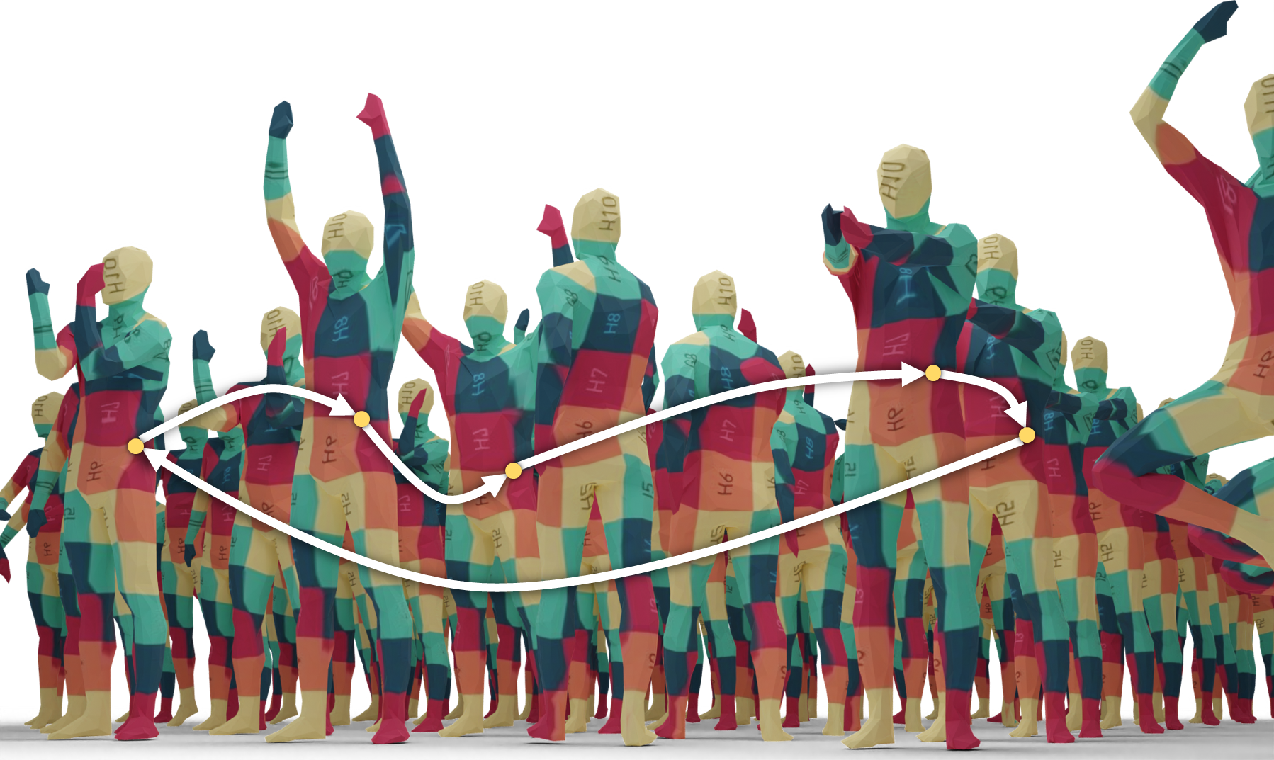
Figure 1: Our quantum-hybrid method matches all $\boldsymbol{100}$ shapes of the FAUST collection [4] with guaranteed cycle consistency (white arrows). Here, we visualise the matchings via texture transfer between all shapes. Our method scales linearly in the number of shapes. See the full figure in the supplement.

A recent example for such a problem is shape matching, where the goal is to estimate correspondences between two shapes. Accurate shape matching is a core element of many computer vision and graphics applications (i.e., texture transfer and statistical shape modelling). If non-rigid deformations are allowed, even pairwise matching is $\mathcal{NP}$-hard, leading to a wide area of research that approximates this problem, as a recent survey shows [18]. Matching two shapes is one of the problems that was shown to benefit from quantum hardware: Q-Match [42] iteratively updates a subset of point correspondences using QA. Specifically, its cyclic $\alpha$-expansion allows to parametrise changes to permutation matrices without relaxations.

The question we ask in this work is: How can we design a multi-shape matching algorithm in the style of Q-Match that has the same benefits? As we show in the experiments, where we introduce several naïve multi-shape extensions of Q-Match, this is a highly non-trivial task. Despite tweaking them, our proposed method significantly outperforms them.

If $N{>}2$ shapes have to be matched, the computational complexity of naïve exhaustive pairwise matching increases quadratically with $N$, which does not scale to large $N$. Furthermore, these pairwise matchings can easily turn out to be inconsistent with each other, thereby violating cycle consistency. For example, chaining the matchings $P_{\mathcal{X}\mathcal{Y}}$ from shape $\mathcal{X}$ to $\mathcal{Y}$ and $P_{\mathcal{Y}\mathcal{Z}}$ from $\mathcal{Y}$ to $\mathcal{Z}$ can give very different correspondences between $\mathcal{X}$ and $\mathcal{Z}$ than the direct, pairwise matching $P_{\mathcal{X}\mathcal{Z}}$ of $\mathcal{X}$ and $\mathcal{Z}$: $P_{\mathcal{X}\mathcal{Z}}\neq P_{\mathcal{X}\mathcal{Y}}P_{\mathcal{Y}\mathcal{Z}}$. (We apply the permutation matrix $P_{\mathcal{X}\mathcal{Y}}$ to the one-hot vertex index vector $x\in\mathcal{X}$ as $x^{\top}P_{\mathcal{X}\mathcal{Y}}=y\in\mathcal{Y}$.) Thus, how can we achieve cycle consistency by design? A simple solution would be to match a few pairs in the collection to create a spanning tree covering all shapes and infer the remaining correspondences by chaining along the tree. Despite a high accuracy of methods for matching two shapes, this correspondence aggregation policy is prone to error accumulation [39]. A special case of this policy is pairwise matching against a single anchor shape, which also guarantees cycle-consistent solutions by construction [22]. We build on this last option in our method as it avoids error accumulation.

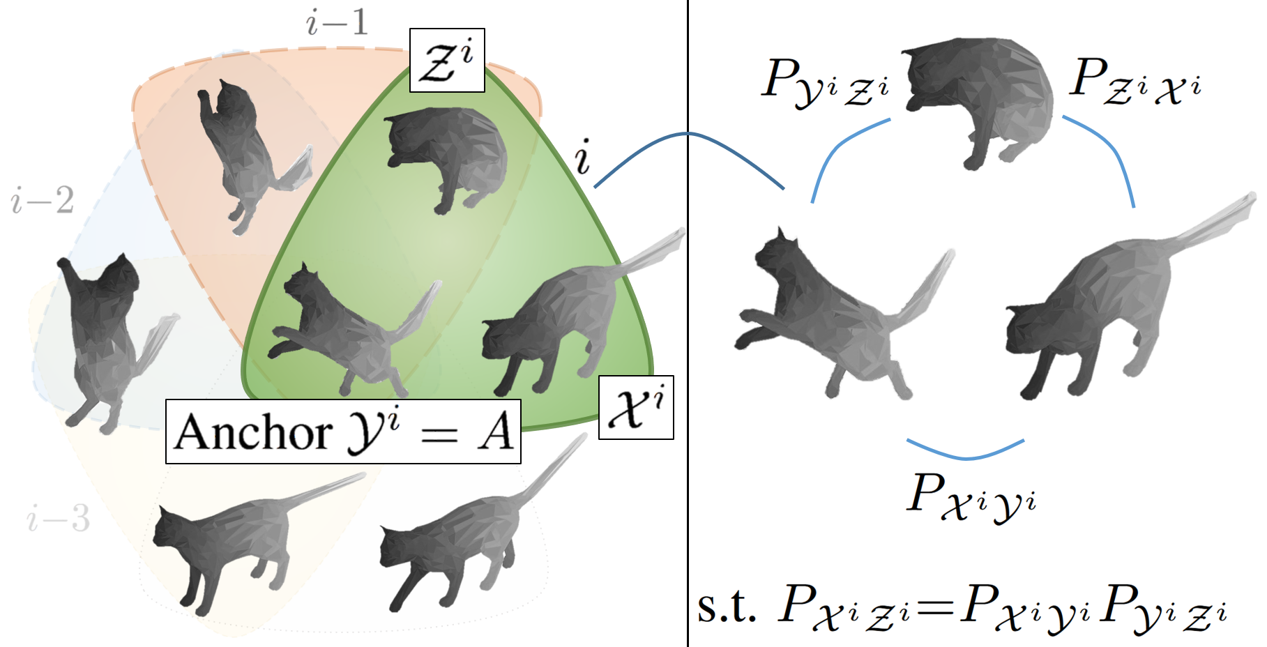
Figure 2: We match $N$ shapes by iteratively matching triplets.

This paper, in contrast to purely classical methods, leverages the advantages of quantum computing for multi-shape matching and introduces a new method for simultaneous alignment of multiple meshes with guaranteed cycle consistency; see Fig. 1. It makes a significant step forward compared to Q-Match and other methods utilising adiabatic quantum computing (AQC), the basis for QA. Our cycle-consistent quantum-hybrid multi-shape matching (CCuantuMM; pronounced “quantum”) approach relies on the computational power of modern quantum hardware. Thus, our main challenge lies in casting our problem in QUBO form, which is necessary for compatibility with AQC. To that end, two design choices are crucial: (1) Our method reduces the $N$-shapes case to a series of three-shape matchings; see Fig. 2. Thus, CCuantuMM is iterative and hybrid, i.e., it alternates in every iteration between preparing a QUBO problem on the CPU and sampling a QUBO solution on the AQC. (2) It discards negligible higher-order terms, which makes mapping the three-shape objective to quantum hardware possible. In summary, the core technical contributions of this paper are as follows:

• CCuantuMM, i.e., a new quantum-hybrid method for shape multi-matching relying on cyclic $\alpha$-expansion. CCuantuMM produces cycle-consistent matchings and scales linearly with the number of shapes $N$.

• A new formulation of the optimisation objective for the three-shapes case that is mappable to modern QA.

• A new policy in shape multi-matching to address the $N$-shape case relying on a three-shapes formulation and adaptive choice of an anchor shape.

Our experiments show that CCuantuMM significantly outperforms several variants of the previous quantum-hybrid method Q-Match [42]. It is even competitive with several non-learning-based classical state-of-the-art shape methods [36, 22] and can match more shapes than them. In a broader sense, this paper demonstrates the very high potential of applying (currently available and future) quantum hardware in computer vision.

2 Related Work

Quantum Computer Vision (QCV). Several algorithms for computer vision relying on quantum hardware were proposed over the last three years for such problems as shape matching [23, 42, 35], object tracking [32, 47], fundamental matrix estimation, point triangulation [20] and motion segmentation [1], among others. The majority of them address various types of alignment problems, i.e., transformation estimation [23, 35], point set [23, 37] and mesh alignment [42], graph matching [41, 3] and permutation synchronisation [3].

Only one of them, QSync [3], can operate on more than two inputs and ensure cycle consistency for the underlying matchings. In contrast to QSync, we can align inputs with substantially larger (by two orders of magnitude) shapes in the number of vertices. Furthermore, we address a different problem, i.e., mesh alignment, for which an algorithm for two-mesh alignment with the help of AQC exists, namely Q-Match [42], as we discuss in the introduction.

To maintain the valid structure of permutation matrices, Quantum Graph Matching, QGM[41] and Q-Sync [3] impose linear constraints. However, this requires that the corresponding penalty parameter is carefully chosen. If the parameter is chosen too big and the linear constraints are enforced too strongly, this severely limits QGM and Q-Sync’s ability to handle large sets of vertices. On the other hand, if the linear constraints are enforced too weakly, there is no guarantee to obtain valid permutations as solutions. As discussed in the introduction, our approach follows Q-Match to ensure valid permutation matrices by construction.

Multi-Shape Matching. We focus this section on multi-shape and non-learning methods as CCuantuMM falls in this category. As our approach is not learning-based, it trivially generalises to unknown object categories without a need for training data. For a general survey of recent advances in shape matching, see Sahillioglu [40].

Matching shape pairs is a classical problem in geometry processing [36]. When more than two shapes of the same class exist, stronger geometric cues can be leveraged to improve results by matching all of them simultaneously. Unfortunately, the already very high problem complexity increases even further the more shapes are used. Hence, existing multi-shape matching methods limit the total number of shapes and their resolution [12, 22], work in spectral space [26], or relax the permutation constraints [28]. Early multi-matching methods computed pair-wise matchings and subsequently used permutation synchronisation to establish cycle consistency [38, 33, 43]. Still, permutation synchronisation requires the eigendecomposition of a matrix with quadratically increasing dimensions [38].

HiPPI [2] is a computationally efficient method that takes geometric relations into account while generalising permutation synchronization but is still limited in resolution. Instead of looking at permutations directly, ZoomOut [36] reduces the dimensionality of the problem by projecting it onto the spectral decomposition. This idea has been extended to take cycle consistency within the spectral space into account [25], which does not guarantee a point-wise consistent matching. To circumvent this issue, IsoMuSh [22] jointly optimises point and functional correspondences. The method detangles the optimisation into smaller subproblems by using a so-called universe shape that all shapes are mapped to instead of each other, as Cao and Bernard do [10]. Using a universe is similar to requiring a template shape, as many learning-based approaches do [24, 19, 44]: Both synchronise all correspondences by matching them through a unified space. This is similar to the concept of anchor shape we use but inherently less flexible because the universe size or template have to be given a priori. Our anchor is chosen from the given collection as part of the method. Although using an anchor slightly improves our results, we note that our method does not necessarily require one for operation. Hence, a random shape could be picked instead in each iteration without an increase in complexity if using an anchor is not feasible or does not represent the shape collection well.

3 Background

3.1 Adiabatic Quantum Computing (AQC)

AQC is a model of computation that leverages quantum effects to obtain high-quality solutions to the $\mathcal{NP}$-hard problem class of Quadratic Unconstrained Binary Optimisation (QUBO) problems: $\min_{x\in\{0,1\}^{k}}x^{T}Qx$, for $k\in\mathbb{N}$ and a QUBO weight matrix $Q\in\mathbb{R}^{k\times k}$. Each entry of $x$ corresponds to its own logical qubit, the quantum equivalent of a classical bit. The diagonal of $Q$ consists of linear terms, while the off-diagonals are inter-qubit coupling weights. A QUBO can be classically tackled with simulated annealing (SA) [45] or a variety of other discrete optimisation techniques [31, 21], which, for large $k$, typically yield only approximate solutions as QUBOs are in general $\mathcal{NP}$-hard. AQC holds the potential to systematically outperform classical approaches such as SA, see [17, 30] for an example. AQC exploits the adiabatic theorem of quantum mechanics [5]: If, when starting from an equal superposition state of the qubits (where all solutions $\{0,1\}^{k}$ have the same probability of being measured) and imposing external influences corresponding to the QUBO matrix on the qubits sufficiently slowly (called annealing), they will end up in a quantum state that, when measured, yields a minimizer $x$ of the QUBO. Not all physical qubits on a real quantum processing unit (QPU) can be connected (coupled) with each other. Thus, a minor embedding of the logical-qubit graph (defined by non-zero entries of the QUBO matrix) into the physical-qubit graph (defined by the hardware) is required [9]. This can lead to a chain of multiple physical qubits representing a single logical qubit. For details of quantum annealing on D-Wave machines, we recommend [34].

3.2 Shape Matching

The problem of finding a matching for non-rigidly deformed shapes having $n$ vertices can be formulated as an $\cal NP$-hard Quadratic Assignment Problem (QAP) [28, 8]:

$$\min_{P\in\mathbb{P}_{n}}p^{T}Wp,$$ (1)

where $p=\text{vec}(P)\in\{0,1\}^{n^{2}}$ is a flattened permutation matrix, and $W\in\mathbb{R}^{n^{2}\times n^{2}}$ is an energy matrix describing how well certain pairwise properties are conserved between two pairs of matches. If two shapes $\cal X,\cal Y$ are discretised with $n$ vertices each, $W$ is often chosen as [28]:

$$W_{x_{1}\cdot n+y_{1},x_{2}\cdot n+y_{2}}=\|d_{\cal X}^{g}(x_{1},x_{2})-d_{\cal Y}^{g}(y_{1},y_{2})\|,$$ (2)

where $x_{1},x_{2}$ are vertices on $\cal X$; $y_{1},y_{2}$ are vertices on $\cal Y$; and $d_{\cal I}^{g}(\cdot,\cdot)$ is the geodesic distance on the shape $\cal I$. Therefore, $W_{x_{1}\cdot n+y_{1},x_{2}\cdot n+y_{2}}$ represents how well the geodesic distance is preserved between corresponding pairs of vertices on the two shapes. Instead of pure geodesics, Gaussian-filtered geodesics are also a popular choice for $W$ [46]:

$$g_{\cal X}(x_{1},x_{2})=\frac{1}{\rho\sqrt{2\pi}}\exp{\left(-\frac{1}{2}\left(\frac{d^{g}_{\cal X}(x_{1},x_{2})}{\rho}\right)^{2}\right)}.$$ (3)

$g_{\mathcal{I}}$ can be used to directly replace $d^{g}_{\mathcal{I}}$ in (2). A small value of $\rho$ focuses the energy on a local neighbourhood around the vertex, while a large value increases the receptive field. Using Gaussian kernels in $W$ places more emphasis on local geometry whereas geodesics have higher values far away from the source vertex. Thus, geodesics work well for global alignment and Gaussians for local fine-tuning.

3.3 Cyclic $\boldsymbol{\alpha}$-Expansion (CAE)

CCuantuMM represents matchings as permutation matrices. In order to update them, we build on Seelbach et al.’s CAE algorithm [42] (similar to a fusion move [27]), which we describe here. A permutation matrix $P$ is called an $r$-cycle, if there exist $r$ disjoint indices $i_{1},\ldots,i_{r}$ such that $P_{i_{j}i_{(j+1)\%r}}=1$ for all $j\in\{1,\ldots,r\}$ and $P_{l,l}=1$ for all $l\notin\{i_{1},\ldots,i_{r}\}$, in which case $P=(i_{1}i_{2}\ldots i_{r})$ is a common notation. Two cycles, i.e. two permutation matrices, are disjoint if these indices are pairwise disjoint. We know that disjoint cycles commute, which allows us to represent any permutation $P$ as $P=\left(\prod_{i=1}^{k}c_{i}\right)\left(\prod_{i=1}^{l}\tilde{c}_{i}\right)$, where $\{c_{i}\}_{i}$ and $\{\tilde{c}_{i}\}_{i}$ each are sets of disjoint $2$-cycles.

Given a set $\{c_{i}\}_{i=1}^{k}$ of $k$ disjoint $2$-cycles, an update, or modification, of $P$ can therefore be parameterised as: $P(\alpha)=\prod_{i=1}^{k}c_{i}^{\alpha_{i}}P,$ where $\alpha\in\{0,1\}^{k}$ is a binary decision vector determining the update. (Note that $\alpha_{i}$ in $c_{i}^{\alpha_{i}}$ is an exponent, not an index.) Crucially, to make this parameterisation compatible with QUBOs, we need to make it linear in $\alpha$. To this end, CAE uses the following equality:

$$P(\alpha)=P+\sum_{i=1}^{k}\alpha_{i}(c_{i}-I)P.$$ (4)

4 Our CCuantuMM Method

Previous adiabatic quantum computing methods [41, 42] can only match two shapes. We present a method for matching $N$ shapes. To ensure cycle consistency on $N$ shapes, it is sufficient that all triplets of shapes are matched cycle consistently [25]. CCuantuMM iteratively solves three-shape problems, which preserve cycle consistency by construction and fit on existing quantum annealers with limited resources. We introduce our formulation for matching three shapes in Sec. 4.1 and then extend it to $N$ shapes in Sec. 4.2.

4.1 Matching Three Shapes

Consider the problem of matching three non-rigidly deformed shapes $\mathcal{S}=\{\mathcal{X,Y,Z}\}$ of $n$ vertices each, while preserving cycle consistency. We formulate this as an energy minimisation with respect to $\mathcal{P}=\{P_{\cal IJ}\in\mathbb{P}_{n}|\cal I,J\in\cal S\}$, the set of permutations between all pairs in $\mathcal{S}$:

$$\min_{\mathcal{P}}\sum_{\cal I,J\in\mathcal{S};\cal I\neq\cal J}\operatorname{vec}(P_{\cal IJ})^{\top}W_{\cal IJ}\operatorname{vec}(P_{\cal IJ}),$$ (5)

$$\textrm{s.t. }\quad P_{\cal XZ}=P_{\cal XY}P_{\cal YZ},$$

where $W_{\cal IJ}\in\mathbb{R}^{n^{2}\times n^{2}}$ is the energy matrix describing how well certain pairwise properties are conserved between shapes $\cal I$ and $\cal J$ (see Sec. 3.2), and $P_{\cal XZ}=P_{\cal XY}P_{\cal YZ}$ enforces cyclic consistency. An overview of the algorithm for three shapes is shown in Alg. 1.

4.1.1 QUBO Derivation

To perform optimisation on the quantum annealer, we need to transform (LABEL:eq:ThreeMatch) into a QUBO problem. We adapt the CAE formulation from [42] (see Sec. 3.3) and iteratively update the permutations to decrease the value of (LABEL:eq:ThreeMatch). Given a set $C=\{c_{i}\}_{i=1}^{k}$ of $k$ disjoint 2-cycles and binary decision variables $\alpha$, we can parameterise our permutation matrices as $P_{\cal IJ}(\alpha)=P_{\cal IJ}+\sum_{i=1}^{k}\alpha_{i}(c_{i}-I)P_{\cal IJ}$. However, CAE alone is not sufficient to transform (LABEL:eq:ThreeMatch) into a QUBO as cyclic consistency is still missing. A simple solution would be to encourage cyclic consistency as a quadratic soft penalty, but then there are no guarantees on the solution. Instead, we enforce cyclic consistency by construction:

$$P_{\cal XZ}(\alpha,\beta)=$$ (6)

$$(P_{\cal XY}+\sum_{i=1}^{k}\alpha_{i}(c_{i}-I)P_{\cal XY})\cdot(P_{\cal YZ}+\sum_{j=1}^{k}\beta_{j}(\tilde{c}_{j}-I)P_{\cal YZ}),$$

where $\{c_{i}\}_{i}$ $\left(\{\tilde{c}_{j}\}_{j}\right)$ are cycles and $\alpha$ ($\beta$) are decision variables for the updates to $P_{\cal XY}$ ($P_{\cal YZ}$). For brevity, we write $C_{i}=(c_{i}-I)P_{\cal XY}$ and $\tilde{C_{j}}=(\tilde{c}_{j}-I)P_{\cal YZ}$. We explain how we construct the cycles in Secs. 4.1.2-4.1.3. Thus, we iteratively solve (LABEL:eq:ThreeMatch) via a sequence of problems of the form:

$$\min_{\alpha,\beta\in\{0,1\}^{k}}{\color[rgb]{1.0,0.55,0.0}E_{\cal XY}(P_{\cal XY}(\alpha))}+{\color[rgb]{0,0,1}E_{\cal YZ}(P_{\cal YZ}(\beta))}+{\color[rgb]{0.0,0.55,0.0}E_{\cal XZ}({P_{\cal XZ}(\alpha,\beta))}},$$ (7)

where $E_{\cal IJ}(P,Q)=$ $\operatorname{vec}(P)^{\top}W_{\cal IJ}\operatorname{vec}(Q)$ and $E_{\cal IJ}(P)=$ $E_{\cal IJ}(P,P)$. While the first two terms are in QUBO form, the third term contains cubic and bi-quadratic terms (see the supplement for details) which are not compatible with current quantum annealer architectures.

Higher-Order Terms.

All of these higher-order terms come from $P_{\cal XZ}(\alpha,\beta)$, specifically from the term $H=\sum_{i}\sum_{j}\alpha_{i}\beta_{j}C_{i}\tilde{C}_{j}$. As we only consider 2-cycles, $C_{i}$ and $\tilde{C}_{j}$ each have only four non-zero elements. Due to this extreme sparsity, most summands of $H$ become $0$.

We could tackle these undesirable terms by decomposing them into quadratic terms by using ancilla variables and adding penalty terms [16]. This gives exact solutions for sufficiently high weights of the penalty terms. However, multiple reasons speak against this: (1) the QUBO matrix is already dense (a clique) under the current formulation (as we will see in (9)) and adding ancilla qubits scales quadratically in $k$, (2) adding penalties makes the problem harder to solve, and (3) $H$ is sparsely non-zero and in practise we observe no drastic influence on the quality of the solution.

Alternatively, we could assume $H{=}0$. However, this is unnecessarily strong since (1) $H$ also contributes to quadratic terms ($E(H,\cdot)$), and (2) higher-order terms operating on the same decision variable trivially reduce to quadratic terms: $\alpha_{i}\cdot\alpha_{i}=\alpha_{i}$ for binary $\alpha_{i}$. We thus keep those two types of terms and merely assume all truly cubic and bi-quadratic terms to be zero.

Cycle-Consistent CAE.

After eliminating the higher-order terms and ignoring constants from (7), we obtain (with the same colour coding):

$$\min_{\alpha,\beta}\quad\sum_{i=1}^{k}\alpha_{i}\bigg{(}{\color[rgb]{1.0,0.55,0.0}F_{\cal XY}(P_{\cal XY},C_{i})}+{\color[rgb]{0.0,0.55,0.0}F_{\cal XZ}(P_{\cal XZ},C_{i}P_{\cal YZ})}\bigg{)}$$ (8)

$$+\sum_{j=1}^{k}\beta_{j}\bigg{(}{\color[rgb]{0,0,1}F_{\cal YZ}(P_{\cal YZ},\tilde{C}_{j})}+{\color[rgb]{0.0,0.55,0.0}F_{\cal XZ}(P_{\cal XZ},P_{\cal XY}\tilde{C}_{j})}\bigg{)}$$

$$+\sum_{i=1}^{k}\sum_{l=1}^{k}\alpha_{i}\alpha_{l}\bigg{(}{\color[rgb]{1.0,0.55,0.0}E_{\cal XY}(C_{i},C_{l})}+{\color[rgb]{0.0,0.55,0.0}E_{\cal XZ}(C_{i}P_{\cal YZ},C_{l}P_{\cal YZ})}\bigg{)}$$

$$+\sum_{j=1}^{k}\sum_{l=1}^{k}\beta_{j}\beta_{l}\bigg{(}{\color[rgb]{0,0,1}E_{\cal YZ}(\tilde{C}_{j},\tilde{C}_{l})}+{\color[rgb]{0.0,0.55,0.0}E_{\cal XZ}(P_{\cal XY}\tilde{C}_{j},P_{\cal XY}\tilde{C}_{l})}\bigg{)}$$

$$+\sum_{i=1}^{k}\sum_{j=1}^{k}\alpha_{i}\beta_{j}\bigg{(}{\color[rgb]{0.0,0.55,0.0}F_{\cal XZ}(P_{\cal XY}\tilde{C}_{j},C_{i}P_{\cal YZ})}+{\color[rgb]{0.0,0.55,0.0}F_{\cal XZ}(K_{ij},P_{\cal XZ})}$$

$$+{\color[rgb]{0.0,0.55,0.0}F_{\cal XZ}(K_{ij},P_{\cal XY}\tilde{C}_{j})}+{\color[rgb]{0.0,0.55,0.0}F_{\cal XZ}(K_{ij},C_{i}P_{\cal YZ})}+{\color[rgb]{0.0,0.55,0.0}E_{\cal XZ}(K_{ij},K_{ij})}\bigg{)},$$

where $P_{\cal XZ}=$ $P_{\cal XZ}(\mathbf{0},\mathbf{0})=$ $P_{\cal XY}P_{\cal YZ}$, and we use the shorthands $F_{\cal IJ}(A,B)=$ $E_{\cal IJ}(A,B)+E_{\cal IJ}(B,A)$ and $K_{ij}=$ $C_{i}\tilde{C}_{j}$. Denoting $\alpha_{k+j}=\beta_{j}$ for an expanded $\alpha\in\{0,1\}^{2k}$, (8) can be written in the form:

$$\min_{\alpha\in\{0,1\}^{2k}}\quad\alpha^{\top}\tilde{W}\alpha.$$ (9)

The full formula for $\tilde{W}$ is provided in the supplement. (9) is finally in QUBO form and we can optimise it classically or on real quantum hardware (see Sec. 3.1).

4.1.2 Choosing Vertices

The question of how to choose the sets of cycles $\{c_{i}\}_{i},\{\tilde{c}_{j}\}_{j}$ is still open. We first choose a subset of vertices using the “worst vertices” criterion introduced in [42] based on the relative inconsistency $I_{\cal XY}$ of a vertex $x\in\mathcal{X}$ under the current permutation:

$$I_{\cal XY}(x)=\sum_{w\in\cal X}W_{x\cdot n+x^{\top}P_{\cal XY},w\cdot n+w^{\top}P_{\cal XY}},$$ (10)

where we treat the one-hot vector $x^{\top}P_{\cal XY}$ as a vertex index on $\cal Y$. A high value indicates that $x$ is inconsistent with many other matches under $P_{\cal XY}$ and swapping it will likely improve the matching. We denote the set of the $m{=}2k$ vertices with the highest $I_{\cal XY}(\cdot)$ as $V_{\cal X}$. Finally, we follow the permutations to get $V_{\cal Y}=\{x^{\top}P_{\cal XY}|x\in V_{\cal X}\}\subset{\cal Y}$.

In practice, we observe a systematic improvement in the matchings when considering all three possibilities (using $I_{\cal XY}$, $I_{\cal YZ}$, or $I_{\cal XZ}$ as the starting point). We thus use three “sub”-iterations per iteration, one for each possibility.

4.1.3 Choosing Cycles

Figure 3: We depict the sub-iteration that starts from $I_{\cal XY}$, from which we construct $V_{\mathcal{X}}$, then $\mathcal{C}^{\mathit{all}}_{\cal X}$, and finally $\mathcal{C}_{\cal X}=$ $\{\mathcal{C}^{0}_{\cal X},$ $\mathcal{C}^{1}_{\cal X},$ $\mathcal{C}^{2}_{\cal X}\}$. We also build $V_{\mathcal{Y}}$ from $V_{\mathcal{X}}$ and construct $\mathcal{C}_{\cal Y}$ analogously. Matching each element of $\mathcal{C}_{\cal X}$ with one from $\mathcal{C}_{\cal Y}$ (visualised via matching colours) leads to three sub-sub-iterations.

Figure 4: We depict the sub-sub-iteration for $\mathcal{C}_{\cal X}^{2}=$ $\{(u_{x},v_{x}),$ $(w_{x},t_{x})\}$ and $\mathcal{C}_{\cal Y}^{1}=\{(u_{y},w_{y}),(v_{y},t_{y})\}$ from Fig. 3.

Given the worst vertices $V_{\cal X}$ and $V_{\cal Y}$ of any sub-iteration, we construct the cycles $\{c_{i}\}_{i},\{\tilde{c}_{j}\}_{j}$ from them. Fig. 3 visualises this process. Focusing on $V_{\cal X}$ for the moment, we want to use all possible 2-cycles $\mathcal{C}_{\mathcal{X}}^{\mathit{all}}=\{(uv)|u,v\in V_{\cal X},u\neq v\}$ in each sub-iteration. We cannot use all of these cycles at once since they are not disjoint, as CAE requires. Instead, we next construct a set $\mathcal{C}_{\cal X}$ by partitioning $\mathcal{C}_{\mathcal{X}}^{\mathit{all}}$ into $m{-}1$ sets of cycles with each containing $m/2{=}k$ disjoint cycles. An analogous methodology is used for $\mathcal{C_{Y}}$.

We now have $\mathcal{C_{X}}$ and $\mathcal{C_{Y}}$. Since we want to consider each cycle of $\mathcal{C}_{\mathcal{X}}^{\mathit{all}}$ and $\mathcal{C}_{\mathcal{Y}}^{\mathit{all}}$ once, we need several “sub-sub” iterations. Thus, we next need to pick one set of cycles from each $\mathcal{C_{X}}$ and $\mathcal{C_{Y}}$ for each sub-sub-iteration. There are $(m{-}1)^{2}$ possible pairs between elements of $\mathcal{C_{X}}$ and $\mathcal{C_{Y}}$. Considering all possible pairs is redundant, does not provide significant performance advantage, and increases the computational complexity quadratically. Hence, we randomly pair each element of $\mathcal{C}_{\cal X}$ with one element of $\mathcal{C}_{\cal Y}$ (without replacement). This leads to $m{-}1$ sub-sub-iterations, with each one solving (9) with its respective cycles; see Fig. 4.

Algorithm 1 Hybrid Three-Shape Matching

Input: $\mathcal{P}^{i},\mathcal{S}$
Output: $\mathcal{P}^{i+1}$

1:for $I\in\{I_{\cal XY},I_{\cal YZ},I_{\cal XZ}\}$ do $\triangleright$ sub-iterations

2:     construct $V_{\cal X},V_{\cal Y},V_{\cal Z}$ (see Sec. 4.1.2)

3:     construct $\cal C_{X},C_{Y},C_{Z}$ (see Sec. 4.1.3)

4:     for $l{=}1$ to $m{-}1$  do $\triangleright$ sub-sub-iterations

5:         compute $\tilde{W}$

6:         optimise QUBO (9) $\triangleright$ quantum

7:     end for

8:     $P_{\cal XY}=\prod_{i=1}^{k}c_{i}^{\alpha_{i}}P_{\cal XY}$

9:     $P_{\cal YZ}=\prod_{j=1}^{k}\tilde{c}_{j}^{\alpha_{m+j}}P_{\cal YZ}$

10:     $P_{\cal XZ}=P_{\cal XY}\cdot P_{\cal YZ}$

11:end for

12:return $\mathcal{P}^{i+1}=\{P_{\cal XY},P_{\cal YZ},P_{\cal XZ}\}$

4.2 Matching $N$ Shapes

In this section, we extend our model to matching a shape collection $\mathcal{S}$ with $N$ elements by iteratively matching three shapes while still guaranteeing cycle consistency. Similar to the three-shape case (LABEL:eq:ThreeMatch), this can be formulated as an energy minimisation problem with respect to the set of permutations $\mathcal{P}$, except $\mathcal{S}$ now has cardinality $N$:

$$\min_{\mathcal{P}} \sum_{\mathcal{I},\mathcal{J}\in\mathcal{S};\mathcal{I}\neq\mathcal{J}}E_{\cal IJ}(P_{\cal IJ}),$$ (11)

s.t. $$P_{\cal IK}=P_{\cal IJ}P_{\cal JK}\quad\forall\mathcal{I,J,K}\in\mathcal{S}.$$

The energy contains summands for each possible pair of shapes. Solving all of them jointly would be computationally expensive and even more complicated than (8). This is the reason most multi-shape matching methods apply relaxations at this point or cannot scale to a large $N$. However, the cycle-consistency constraints still only span over three shapes; triplets are sufficient for global consistency [25].

We thus iteratively focus on a triplet $\mathcal{X},\mathcal{Y},\mathcal{Z}\in\mathcal{S}$ and its set of permutations $\mathcal{P}^{\prime}=\{P_{\mathcal{X}\mathcal{Y}},P_{\mathcal{X}\mathcal{Z}},P_{\mathcal{Y}\mathcal{Z}}\}$. We could then minimise (11) over $\mathcal{P}^{\prime}$, leading to a block-coordinate descent optimisation of (11) over $\mathcal{P}$. This would make the problem tractable on current quantum hardware since it keeps the number of decision variables limited. It would also formally guarantee that our iterative optimisation would never increase the total energy. However, each iteration would be linear in $N$ due to the construction of the QUBO matrix, preventing scaling to large $N$ in practice. We therefore instead restrict (11) to those terms that depend only on permutations from $\mathcal{P}^{\prime}$. This leads to the same energy as for the three-shape case (LABEL:eq:ThreeMatch), where the minimisation is now over $\mathcal{P}^{\prime}$. Importantly, the computational complexity per triplet becomes independent of $N$, allowing to scale to large $N$. While this foregoes the formal guarantee that the total energy never increases, we crucially find that it still only rarely increases in practice; see the supplement.

By iterating over different triples $\mathcal{X}^{i},\mathcal{Y}^{i},\mathcal{Z}^{i}$, we cover the entire energy term and reduce it iteratively. Specifically, one iteration $i$ of the $N$-shape algorithm runs Alg. 1 on $\mathcal{P}^{\prime}=\{P^{i}_{\mathcal{X}^{i}\mathcal{Y}^{i}},P^{i}_{\mathcal{Y}^{i}\mathcal{Z}^{i}},P^{i}_{\mathcal{X}^{i}\mathcal{Z}^{i}}\}$. Here, $\mathcal{X}^{i}$ $\in\mathcal{S}$ is chosen randomly (we use stratified sampling to pick all shapes equally often), the anchor $\mathcal{Y}^{i}=$ $A\in\mathcal{S}$ is fixed, and $\mathcal{Z}^{i}=$ $\mathcal{X}^{i-1}$. In practice, we saw slightly better results with this scheme instead of choosing the triplet randomly; see the supplement. We note that we only need to explicitly keep track of permutations into the anchor: $\mathcal{P}^{i}=\{P^{i}_{\mathcal{I}A}\}_{\mathcal{I}\in\mathcal{S},\mathcal{I}\neq A}$. We then get $\mathcal{P}^{i+1}$ from $\mathcal{P}^{i}$ by replacing $P^{i}_{\mathcal{X}^{i}A}$ and $P^{i}_{\mathcal{Z}^{i}A}$ with their updated versions from Alg. 1.

Initialisation. We compute an initial set of pairwise permutations $\mathcal{P}^{\mathit{init}}$ using a descriptor-based similarity of the normalised heat-kernel-signatures (HKS) [7] extended by a dimension indicating whether a vertex lies on the left or right side of a shape (a standard practice in the shape-matching literature [22]). Instead of using a random shape as anchor, the results improve when using the following shape:

$$A=\operatorname*{arg\,min}_{A\in\mathcal{S}}\sum_{\mathcal{I}\in\mathcal{S};\mathcal{I}\neq A}E_{\mathcal{I}A}(P^{\mathit{init}}_{\mathcal{I}A}),$$ (12)

where $P^{\mathit{init}}_{\mathcal{I}A}\in\mathcal{P}^{\mathit{init}}$. We thus have $\mathcal{P}^{0}=\{P^{\mathit{init}}_{\mathcal{I}A}\}_{\mathcal{I}\in\mathcal{S},\mathcal{I}\neq A}$.

Time Complexity. Our algorithm scales linearly with the number of shapes. Each iteration of Alg. 1 has worst-case time complexity $\mathcal{O}(nk^{3})$, as we discuss in the supplement.

Energy Matrix Schedule. In practise, we first use pure geodesics for a coarse matching and then Gaussian-filtered geodesics to fine-tune. Specifically, for a shape collection of three shapes, we use a schedule with $2T$ geodesics iterations followed by $2T$ Gaussian iterations. For each additional shape in the shape collection, we add $T$ iterations to both schedules. We exponentially decrease the variance of the Gaussians every $N{-}1$ iterations to $\rho(i)=c_{2}\exp(\frac{c_{1}}{i-T})$ where $c_{1}$ and $c_{2}$ are chosen such that the variance decreases from $25\%$ to $5\%$ of the shape diameter over the iterations. Thus, all shapes undergo one iteration with the same specific variance. We refer to the supplement for more details.

5 Experimental Evaluation

We compare against state-of-the-art multi-matching methods with a focus on quantum methods. We consider classical works for reference. All experiments use Python 3.9 on an Intel Core i7-8565U CPU with 8GB RAM and the D-Wave Advantage System 4.1 (accessed via Leap 2). We will release our code, which is accelerated using Numba.

Hyperparameters. We set $T{=}11$. We set the number of worst vertices $m$ to $16\%$ of the number of vertices $n$.

Quantum Comparisons. The closest quantum work, Q-Match [42], matches only two shapes. We consider two adaptations to multi-matching: 1) Q-MatchV2-cc, similar to our CCuantuMM, chooses an anchor and matches the other shapes pairwise to it, implicitly enforcing cycle consistency; and 2) Q-MatchV2-nc matches all pairs of shapes directly, without guaranteed cycle consistency. In both cases, we use our faster implementation and adapt our energy matrix schedule, which gives significantly better results.

Classical Comparisons. For reference, we also compare against the classical, non-learning-based multi-matching state of the art: IsoMuSh [22] and the synchronised version of ZoomOut [36], which both guarantee vertex-wise cycle consistency across multiple shapes.

Evaluation Metric. We evaluate the correspondences using the Princeton benchmark protocol [29]. Given the ground-truth correspondences $P_{\cal IJ}^{*}$ for matching the shape $\mathcal{I}$ to $\mathcal{J}$, the error of vertex $v\in\mathcal{I}$ under our estimated matching $P_{\cal IJ}$ is given by the normalised geodesic distance:

$$e_{v}(P_{\cal IJ})=\frac{d_{\mathcal{J}}^{g}(v^{\top}P_{\cal IJ},v^{\top}P_{\cal IJ}^{*})}{\operatorname{diam}(\mathcal{J})},\quad$$ (13)

where $\operatorname{diam}(\cdot)$ is the shape diameter. We plot the fraction of errors that is below a threshold in a percentage-of-correct-keypoints (PCK) curve, where the threshold varies along the x-axis. As a summary metric, we also report the area-under-the-curve (AUC) of these PCK curves.

Datasets. The FAUST dataset [4] contains real scans of ten humans in different poses. We use the registration subset with ten poses for each class and downsample to $500$ vertices. TOSCA [6] has $76$ shapes from eight classes of humans and animals. We downsample to ${\sim}1000$ vertices. SMAL [48] has scans of toy animals in arbitrary poses, namely $41$ non-isometric shapes from five classes registered to the same template. (E.g., the felidae (cats) class contains scans of lions, cats, and tigers.) We downsample to $1000$ vertices. We use the same number of vertices as IsoMuSh [22], except that they use $1000$ vertices for FAUST.

5.1 Experiments on Real Quantum Annealer

Figure 5: PCK curves for (left) two three-shape and (right) two ten-shape instances using QA and SA. In each plot, we denote one instance by normal lines and the other one by dotted lines.

We run two three-shapes and two ten-shapes experiments with FAUST on a real QPU. However, since our QUBO matrices are dense, we effectively need to embed a clique on the QPU. (The supplement contains a detailed analysis of the minor embeddings and the solution quality.) Hence, we test a reduced version of our method with 20 worst vertices per shape (40 virtual qubits in total), as more would worsen results significantly on current hardware. To compensate for this change, we use more iterations for the ten-shape experiments. We use 200 anneals per QUBO, the default annealing path, and the default annealing time of $20\mu\mathit{s}$. As standard chain strength, we choose $1.0001$ times the largest absolute value of entries in $Q$. Each ten-shape experiment takes about 10 minutes of QPU time. In total, our results took about 30 minutes of QPU time for a total of $5.5\cdot 10^{4}$ QUBOs. QA under these settings achieves a similar performance as SA under the same settings (Fig. 5). As QPU time is expensive and since we have just shown that SA performs comparably to a QPU in terms of result quality, we perform the remaining experiments with SA under our default settings, on classical hardware. This is common practice [42, 1, 47] since SA is conceptually close to QA. For additional results, including results on the new Zephyr hardware [14], we refer to the supplement.

5.2 Comparison to Quantum and Classical SoTA

	Ours	Q-MatchV2-cc	Q-MatchV2-nc	IsoMuSh	ZoomOut	HKS
FAUST	0.989	0.886	0.879	0.974	0.886	0.746
TOSCA	0.967	0.932	0.940	0.952	0.864	0.742
SMAL	0.866	0.771	0.813	0.926	0.851	0.544

Table 1: AUC averaged over all classes of each dataset. For reference, we also include classical methods on the right.

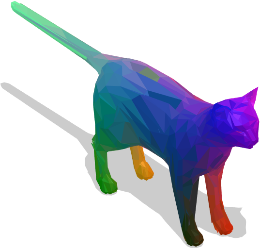
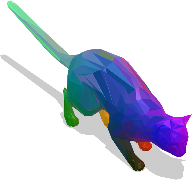
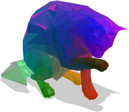
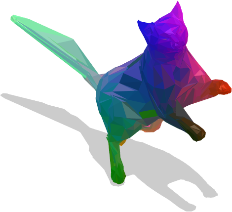
						Ours
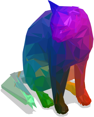
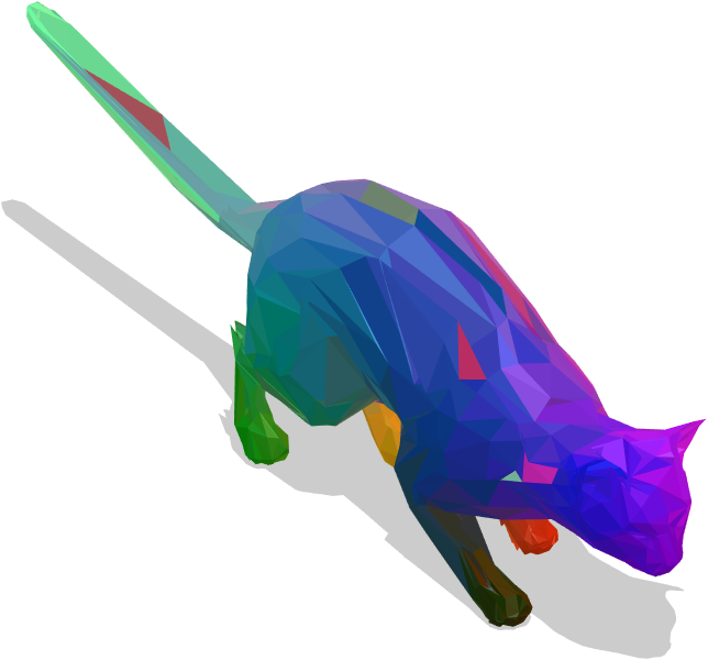
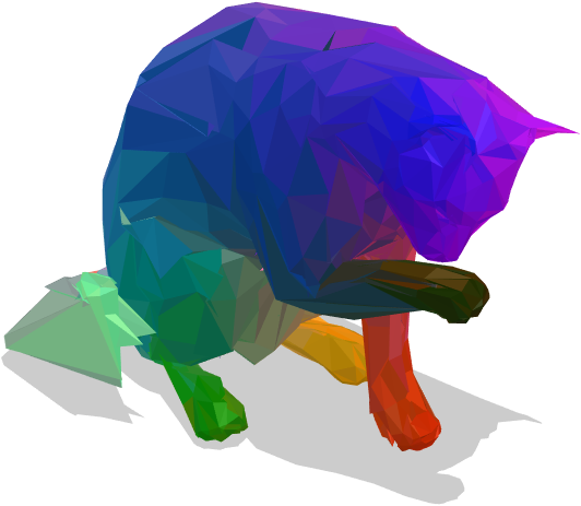
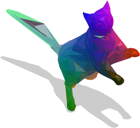
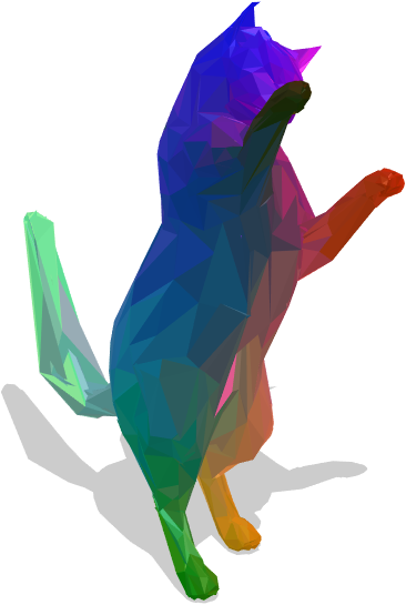
Source						IsoMuSh

Figure 6: Qualitative results on the TOSCA [6] cat class. We colour a source shape and transfer this colouring to target shapes via the matches estimated by our method or IsoMuSh [22].

(a) FAUST [4]

(b) TOSCA [6]

(c) SMAL [48]

Figure 7: Quantitative results on all three datasets. For each dataset, we match all shapes within a class and then plot the average PCK curve across classes. We plot classical methods with dashed lines as they are only for reference. HKS is our initialisation (see Sec. 4.2).

FAUST. We outperform both quantum and classical prior work, as Fig. 7(a) and Tab. 1 show. Because we downsample FAUST more, IsoMuSh’s results are better in our experiments than what Gao et al. [22] report.

Matching $\mathbf{100}$ Shapes. Next, we demonstrate that, unlike IsoMuSh and ZoomOut, our approach can scale to matching all 100 shapes of FAUST. Fig. 1 contains qualitative results. Tab. 2 compares the runtime of our method (using SA) to others. Only ours and Q-MatchV2-cc scale well to $100$ shapes while ZoomOut and IsoMuSh cannot.

# Shapes	Ours	Q-MatchV2-cc	Q-MatchV2-nc	IsoMuSh	ZoomOut
10	97	16	81	$(4+)0.3$	4
100	1137	175	${\sim}8000^{\dagger}$	OOM	OOM

Table 2: Runtime (in min) for FAUST. IsoMuSh uses ZoomOut for initialisation. “OOM” (out of memory): memory requirements are infeasible. “^†” denotes an estimate.

TOSCA. Fig. 7(b) and Tab. 1 show that our method achieves state-of-the-art results. While IsoMuSh’s PCK curve starts higher (better), the AUC in Tab. 1 suggests that our method performs better overall. Fig. 6 has qualitative examples.

SMAL. Our CCuantuMM outperforms the quantum baselines, both in terms of PCK (Fig. 7(c)) and AUC (Tab. 1). At the same time, it achieves performance on par with ZoomOut and below IsoMuSh. SMAL is considered the most difficult of the three datasets due to the challenging non-isometric deformations of its shapes. All methods thus show worse performance compared to FAUST and TOSCA.

5.3 Ablation Studies

We perform an ablation study on FAUST to analyse how different components of our method affect the quality of the matchings. We refer to the supplement for more ablations.

Figure 8: We ablate (left) the usage of Gaussian kernels, and (right) the large-scale multi-shape setting. Gaussian kernels improve the results greatly. Matching more shapes improves results.

Gaussian Energy Schedule. Our schedule, which starts with geodesics and afterwards uses Gaussians, provides a significant performance gain over using only geodesics, under the same number of iterations, see Fig 8. That is because Gaussians better correct local errors in our approach.

Does Using More Shapes Improve Results? We analyse what effect increasing the number of shapes $N$ has on the matchings’ quality. We first randomly select three shapes and run our method on them, to obtain the baseline. Next, we run our method again and again from scratch, each time adding one more shape to the previously used shapes. This isolates the effect of using more shapes from all other factors. In Fig. 8, we plot the PCK curves for the three selected shapes. We repeat this experiment for several randomly sampled instances. Our results show that including more shapes improves the matchings noticeably overall.

5.4 Discussion and Limitations

Our method and all considered methods are based on intrinsic properties like geodesic distances. Thus, without left-right labels for initialisation, they would produce partial flips for inter-class instances in FAUST and intra-class instances in TOSCA and SMAL. For a large worst-vertices set, contemporary quantum hardware leads to embeddings (see Sec. 3.1) with long chains, which are unstable, degrading the result quality. Finally, while our method is currently slower in practice than SA, it would immediately benefit from the widely expected quantum advantage in the future.

6 Conclusion

The proposed method achieves our main goal: improving mesh alignment w.r.t. the quantum state of the art. Furthermore, it is even highly competitive among classical state-of-the-art methods. This suggests that the proposed approach can be used as a reference for comparisons and extensions of classical mesh-alignment works in the future. (For such cases, classical SA is a viable alternative when access to quantum computers is lacking.) Our results show that ignoring certain higher-order terms still allows for high-quality matchings, which is promising for future quantum approaches that could use similar approximations. Finally, unlike classical work, we designed our method within the constraints of contemporary quantum hardware. We found that iteratively considering shape triplets is highly effective, perhaps even for classical methods.

Acknowledgements. This work was partially supported by the ERC Consolidator Grant 4DReply (770784). ZL is funded by the Ministry of Culture and Science of the State of NRW.

Supplementary Material

This supplementary material contains additional results. We present them in the order they are mentioned in the main paper. First, Sec. A provides an overview of our notation. Sec. B formally states the $N$-shape algorithm. Sec. C contains large-scale figures showing the $100$ matched FAUST shapes. Sec. D describes the elimination of higher-order terms in detail. Sec. E states the weight matrix $\tilde{W}$ of the final QUBO. Sec. F shows that the total energy almost never decreases in practice. Sec. G compares our anchor scheme to using random triplets. Sec. H discusses the time complexity of our proposed method. Sec. I provides more implementation details on initialisation and deciding trivial cycles. Sec. J discusses the minor embeddings on real quantum hardware and contains further QPU experiments. Sec. K presents more results, including more ablation experiments. Finally, Sec. L compares existing quantum computer vision works for alignment tasks.

In addition, the supplementary material contains a video showing the evolution of the matchings of a ten-shape FAUST instance over the course of the optimisation. We visualise the matchings by fixing the colouring of the top-left shape and transferring this colouring to all other shapes according to the estimated correspondences.

Appendix A Notations

Tab. 3 summarises the notation we use.

Notation	Meaning
$\mathcal{I}$, $\mathcal{J}$, $\mathcal{X}$, $\mathcal{Y}$, $\cal Z$	shapes (represented as meshes)
$P_{\mathcal{IJ}}$	permutation matrix from shape $\mathcal{I}$ to $\mathcal{J}$
$x$, $y$, $u$, $v$	vertices of a shape
$\mathcal{P}$	set of permutations
$\mathcal{S}$	set of shapes
$W$	energy matrix
$N$	number of shapes
$I$	identity matrix
$E_{\cal IJ}(P,Q)$	$\textit{vec}(P)^{\top}W_{\cal IJ}\textit{vec}(Q)$
$E_{\cal IJ}(P)$	$E_{\cal IJ}(P,P)$
$F_{\cal IJ}(A,B)$	$E_{\cal IJ}(A,B)+E_{\cal IJ}(B,A)$
$\alpha,\beta$	decision variables
$k$	size of decision variables $\alpha$,$\beta$
$m$	number of worst vertices
$I_{\cal XY}(x)$	relative inconsistency of vertex $x$ for $P_{\cal XY}$
$V_{\cal X}$	set of worst vertices for shape $\cal X$
$\mathcal{C_{X}}$	set of cycles for shape $\cal X$
$A$	anchor shape
$C_{i}$	$(c_{i}-I)P_{\cal XY}$; single-cycle update of $P_{\cal XY}$
$\tilde{C}_{j}$	$(c_{j}-I)P_{\cal YZ}$; single-cycle update of $P_{\cal YZ}$
$K_{ij}$	$C_{i}\tilde{C}_{j}$

Table 3: Notation used in this work.

Appendix B $N$-Shape Algorithm

We provide the formal $N$-shape algorithm as Alg. 2.

Algorithm 2 CCuantuMM (Matching $N$ Shapes; Sec. 4.2)

Input: $\mathcal{S},T$
Output: $\mathcal{P}$

1:initialise $\mathcal{P}^{\mathit{init}}$ from HKS descriptors

2:determine anchor $A\in\mathcal{S}$

3:$\mathcal{P}^{0}\leftarrow\{P^{\mathit{init}}_{\mathcal{I}A}\}_{\mathcal{I}\in\mathcal{S},\mathcal{I}\neq A}$

4:randomly pick $\mathcal{X}^{-1}\in\mathcal{S}$$\triangleright$ technicality for $\mathcal{Z}^{0}$

5:for $i=0$ to $2T(\lvert\mathcal{S}\rvert-1)$  do $\triangleright$ iterations

6:     if $i\mod(\lvert\mathcal{S}\rvert-1)==0$ then

7:         $\mathcal{S}^{\prime}\leftarrow\mathcal{S}\setminus\{A\}$$\triangleright$ for stratified sampling

8:     end if

9:     randomly pick $\mathcal{X}^{i}\in\mathcal{S}^{\prime}$

10:     $\mathcal{S}^{\prime}\leftarrow\mathcal{S}^{\prime}\setminus\{\mathcal{X}^{i}\}$

11:     $\mathcal{Y}^{i}\leftarrow A$

12:     $\mathcal{Z}^{i}\leftarrow\mathcal{X}^{i-1}$

13:     get $P^{i}_{\mathcal{X}^{i}A},P^{i}_{\mathcal{Z}^{i}A}$ from $\mathcal{P}^{i}$

14:     $P^{i}_{\mathcal{X}^{i}\mathcal{Y}^{i}}\leftarrow P^{i}_{\mathcal{X}^{i}A}$

15:     $P^{i}_{\mathcal{Y}^{i}\mathcal{Z}^{i}}\leftarrow(P^{i}_{\mathcal{Z}^{i}A})^{-1}$

16:     $P^{i}_{\mathcal{X}^{i}\mathcal{Z}^{i}}\leftarrow P^{i}_{\mathcal{X}^{i}A}(P^{i}_{\mathcal{Z}^{i}A})^{-1}$

17:     $\operatorname{mode}\leftarrow\operatorname{geodesic}$ if $i<T(\lvert\mathcal{S}\rvert-1)$ else $\operatorname{Gaussian}$

18:     $\{P^{i+1}_{\mathcal{X}^{i}\mathcal{Y}^{i}},P^{i+1}_{\mathcal{Y}^{i}\mathcal{Z}^{i}},P^{i+1}_{\mathcal{X}^{i}\mathcal{Z}^{i}}\}\leftarrow$ run Alg. 1 with $\operatorname{mode}$

     on $(\{P^{i}_{\mathcal{X}^{i}\mathcal{Y}^{i}},P^{i}_{\mathcal{Y}^{i}\mathcal{Z}^{i}},P^{i}_{\mathcal{X}^{i}\mathcal{Z}^{i}}\}$, $\{\mathcal{X}^{i},\mathcal{Y}^{i},\mathcal{Z}^{i}\})$

19:     $P^{i+1}_{\mathcal{X}^{i}A}\leftarrow P^{i+1}_{\mathcal{X}^{i}\mathcal{Y}^{i}}$

20:     $P^{i+1}_{\mathcal{Z}^{i}A}\leftarrow(P^{i+1}_{\mathcal{Y}^{i}\mathcal{Z}^{i}})^{-1}$

21:     $\mathcal{P}^{i+1}\leftarrow(\mathcal{P}^{i}\setminus\{P^{i}_{\mathcal{X}^{i}A},P^{i}_{\mathcal{Z}^{i}A}\})\cup\{P^{i+1}_{\mathcal{X}^{i}A},P^{i+1}_{\mathcal{Z}^{i}A}\}$

22:end for

23:return $\mathcal{P}=\mathcal{P}^{2T(\lvert\mathcal{S}\rvert-1)}$

Appendix C Matching $\boldsymbol{100}$ Shapes

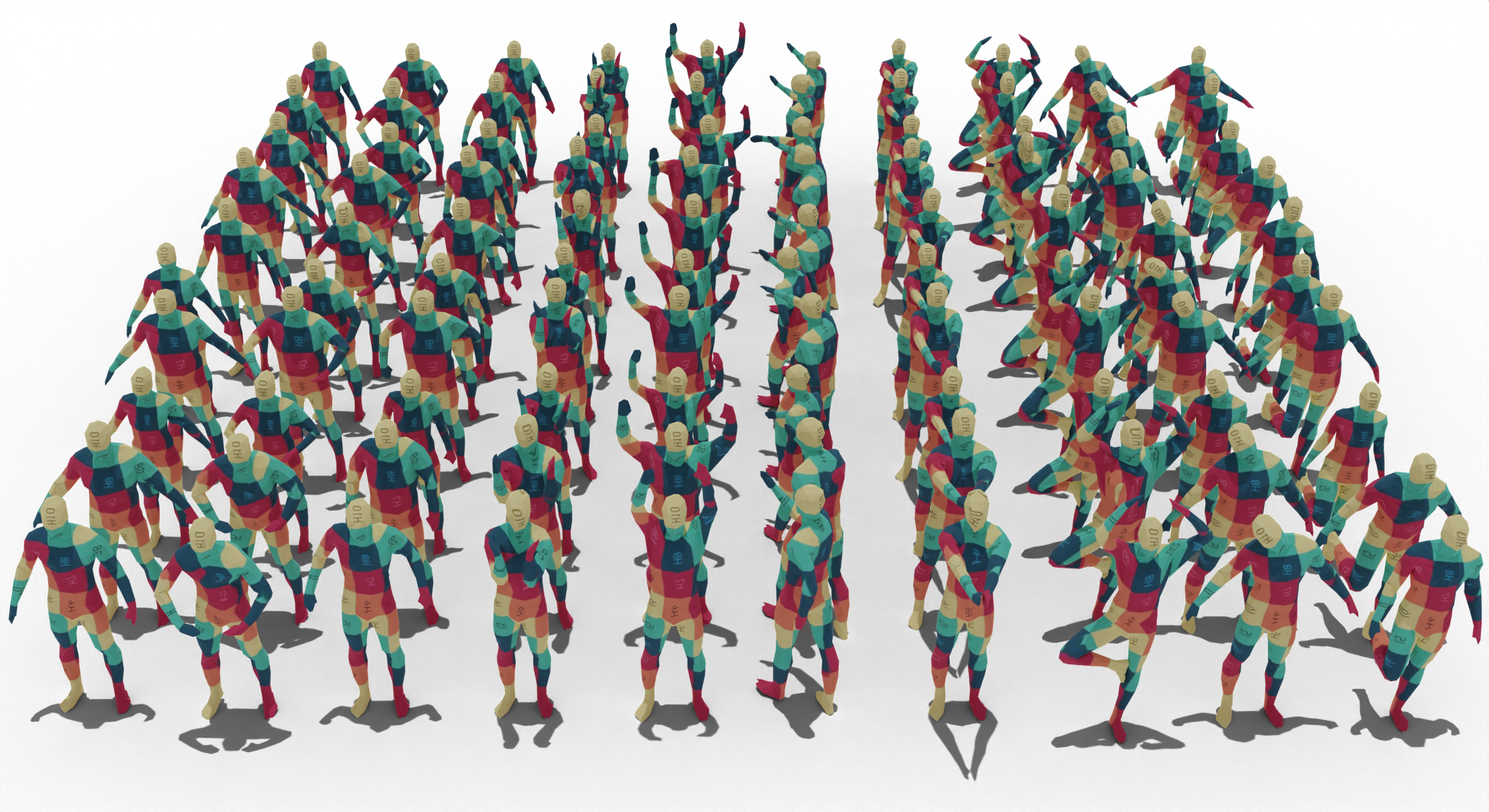
Figure 9: Extended version of Fig. 1 in the main paper. We visualise the matchings between all $100$ FAUST shapes via texture transfer. All correspondences are cycle-consistent by design.

Fig. 9 shows qualitative results of all $100$ matched FAUST shapes.

Appendix D Higher-Order Terms

In this section, we give the expansions for the third term of (7), namely $E_{\cal XZ}(P_{\cal XZ}(\alpha,\beta))$, as it contains higher-order terms. Fig. 20 shows the equations. The terms in red are cubic or bi-quadratic and we hence assume them to be 0, except for the summands that simplify to quadratic terms. For example, $\alpha_{i}\beta_{j}\alpha_{i}\beta_{j}E_{\cal XZ}(C_{i}\tilde{C}_{j},C_{i}\tilde{C}_{j})$ simplifies to the linear summand $\alpha_{i}\beta_{j}E_{\cal XZ}(C_{i}\tilde{C}_{j},C_{i}\tilde{C}_{j})$. This then yields (8) from the main paper.

Appendix E Final QUBO

Fig. 10 shows the weight matrix $\tilde{W}\in\mathbb{R}^{2k\times 2k}$ that is used for the final QUBO.

Figure 10: The final QUBO weight matrix $\tilde{W}$. For indices $i>k$, we define $\tilde{C}_{i}=\tilde{C}_{i-k}$.

Appendix F Evolution During Optimisation

Fig. 11 depicts how the total energy (11) and PCK evolve during optimisation. Importantly, the energy almost never increases in practice. Furthermore, our algorithm converges close to the ground truth. A sudden and significant improvement occurs as soon as the schedule switches from geodesics to Gaussians. We note that although the objective uses Gaussians in the second half of the schedule, both the total energy plotted here and the PCK are based on the (unfiltered) geodesic distances.

(a) FAUST

(b) TOSCA

(c) SMAL

Figure 11: Evolution during the optimisation (left) of the PCK, depicted with a colour bar gradient, and (right) of the total energy. The horizontal red-dashed line is the energy of the ground-truth solution. The results are on (a) a class of FAUST containing ten shapes, (b) the cat class of TOSCA containing eleven shapes, and (c) the cat class of SMAL containing nine shapes.

Appendix G Fixed Anchor vs. Random Triplets

Fig. 12 compares our anchor-based scheme with using random triplets. We see a small improvement with our scheme.

Figure 12: PCK when using a fixed anchor (as our method does) and when using random triplets. We average across all classes of FAUST.

Appendix H Time Complexity

Our method mainly consists of constructing and solving the QUBO matrix $\tilde{W}$, which is based on $W$. However, standard meshes contain thousands of vertices, which makes naïvely calculating the full $W\in\mathbb{R}^{n^{2}\times n^{2}}$ not feasible due to the memory restrictions. Fortunately, we do not need to compute the full $W$ but only a small set of its entries. This is due to the extreme sparsity of the $c_{i}{-}I$ matrix (only four non-zero elements) since we only consider 2-cycles. Using $k$ 2-cycles leads to a worst-case time complexity of $\mathcal{O}(nk^{2})$ for the three-shape Alg. 1 from the main paper (i.e., one sub-sub-iteration). For the sub-sub-iterations of a sub-iteration, $\tilde{W}$ is constant and we thus need to compute $\tilde{W}$ only once for each sub-iteration. In addition, each iteration has $k{-}1$ sub-iterations, resulting in a time complexity of $\mathcal{O}(nk^{3})$ for each iteration. Furthermore, our implementation for computing $\tilde{W}$ is significantly faster in practice than the sub-sampling technique proposed in Q-Match.

Appendix I Implementation Details

I.1 Initialisation

The initial set of permutations $\mathcal{P}^{\mathit{init}}$ is computed using a descriptor-based similarity $\mathit{DS}_{\cal IJ}\in\mathbb{R}^{n\times n}$ between all $n$ vertices of shape pairs $\cal I,J\in\mathcal{S}$. Specifically, $\mathit{DS}_{\cal IJ}(u,v)$ contains the similarity (inner product) of the normalised heat-kernel-signatures (HKS) [7] descriptors (which we extend by an additional dimension indicating whether a vertex lies on the left or right side of a shape) of vertex $u$ of $\cal I$ and vertex $v$ of $\cal J$. The left-right descriptors reduce left-right flips in the solution since the shape classes we consider are globally symmetric, which is not captured by the local HKS descriptors. This is standard practice in the shape-matching literature [22]. The solution of a linear assignment problem on $\mathit{DS}_{\cal IJ}$ is then the initial $P^{\mathit{init}}_{\cal IJ}$.

I.2 Pre-Computing Trivial Cycles

The matrix $\tilde{W}$ consists of couplings (quadratic terms) and linear terms. Numerical experiments show that there often exist cycles with linear terms that dominate the corresponding coupling terms. This happens when a cycle is largely uncorrelated to the rest of the cycles in the current set of cycles. In this case, the decision for such a cycle can be made trivially.

We now derive an inequality for how large the linear term has to be such that the couplings can be neglected in the optimisation problem. Consider the QUBO problem:

$$\min_{\alpha\in\{0,1\}^{k}}\alpha^{T}W\alpha+b^{T}\alpha,$$ (15)

where $\alpha$ are the decision variables, $b\in\mathbb{R}^{k}$ is a vector, and $W$ is a symmetric matrix with zeros on the diagonal representing the couplings. We can look at the terms that depend on $\alpha_{q}$ for fixed $q$ separately:

$$\alpha^{T}W\alpha=\alpha_{q}\sum_{i\neq q}W_{q,i}\alpha_{i}+\alpha_{q}\sum_{i\neq q}\alpha_{i}W_{i,q}$$

$$+\sum_{j\neq q}(\sum_{i\neq q}\alpha_{j}W_{j,i}\alpha_{i}+\alpha_{j}b_{j})+\alpha_{q}b_{q}.$$

As $W$ is symmetric, $W_{i,q}=W_{q,i}$ holds and we can write

$$\alpha^{T}W\alpha=\alpha_{q}\left(b_{q}+2\sum_{i\neq q}W_{q,i}\alpha_{i}\right)$$

$$+\sum_{j\neq q}(\sum_{i\neq q}\alpha_{j}W_{j,i}\alpha_{i}+\alpha_{j}b_{j}).$$

It follows that if:

$$|b_{q}|\geq\sum_{i\neq q}2|W_{q,i}|,$$ (16)

then we can make the decision based on the sign of $b_{q}$: If $b_{q}$ is positive we do not choose the cycle as doing so would increase the energy. This reduces the number of physical qubits required for the embedding.

Appendix J Minor Embeddings and Other QPU Experiments

J.1 QPU Processing and Annealing Time

Optimising a single QUBO uses ${\sim}40ms$ of total QPU processing time for 200 anneals. This is also called the QPU access time [13]. However, there are also several overheads that occur when solving QUBOs by accessing a D-Wave annealer via the cloud. For example, a latency when connecting to the D-Wave annealer and a post processing time. The QPU access time also includes a programming time.

These overheads can be orders of magnitude greater than the time taken by the actual annealing, which is very short since we use the default annealing schedule and the default annealing time of 20 $\mu s$.

J.2 Minor Embeddings

As explained in the main paper, not all physical qubits on a real quantum processing unit (QPU) can be connected (coupled) with each other. Thus, a minor embedding of the logical-qubit graph (defined by non-zero entries of the QUBO matrix) into the physical-qubit graph (defined by the hardware) is required. This can lead to a chain of multiple physical qubits representing a single logical qubit.

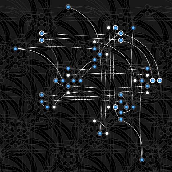
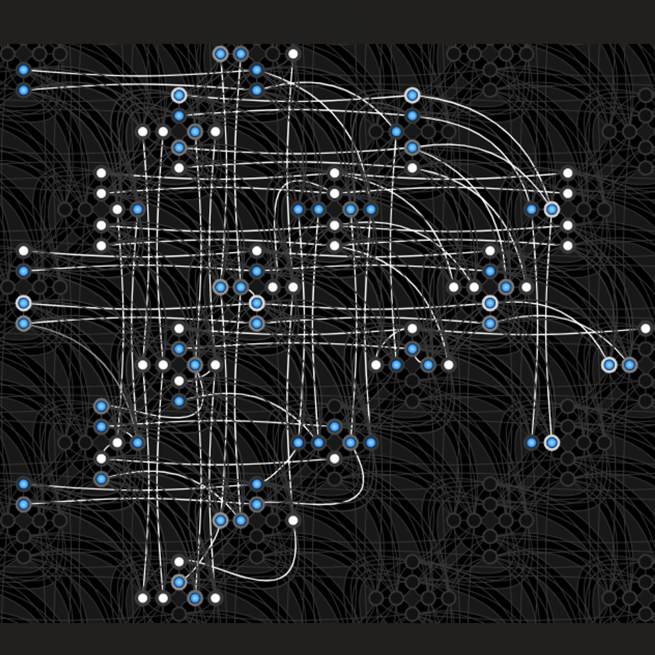
Figure 21: Visualisation of an example minor embedding on Pegasus (which we use in the main paper). The visualisation is obtained via D-Wave Leap 2’s problem inspector [15] for (upper left) 20, (upper right) 30, (lower left) 40, and (lower right) 50 worst vertices. Each node depicts a physical qubit and the edges depict the chains of the minor embeddings.

Our logical input graph is a clique. Due to the limited connectivity of current hardware, a clique cannot be directly embedded onto the physical annealer. We thus require a minor embedding, which is commonly computed using Cai et al.’s method [9]. Fig. 21 visualises an example minor embedding. We note that, since our input graphs are cliques, a generalised embedding can be pre-computed and reused, not impacting the time complexity.

Figure 13: PCK curves for (left) a three-shape and (right) a ten-shape inter-class FAUST instance on both QPU architectures.

Figure 14: Quantitative results when using (solid) 20 and (dashed) 40 worst vertices on a three-shape FAUST instance. We show (left) the energy evolution during optimisation and (right) the final PCK curves.

Figure 15: Structural changes of the minor embeddings when using more worst vertices. We show (left) the number of physical qubits and (right) the average chain length, for both QPU topologies. The number of logical qubits equals the number of worst vertices.

J.3 Minor Embeddings in Practice

In this section, we investigate the empirical impact of minor embeddings on the solutions. The minor embeddings depend on the qubit topology, i.e. the physical qubit connectivity pattern. Here, we show results on the D-Wave Advantage 4.1 with its Pegasus topology (used in the main paper) and also first results on a D-Wave Advantage2 prototype of the next-generation Zephyr topology, which has a higher connectivity than Pegasus.

Fig. 13 shows PCK curves on both topologies when using $m{=}2k{=}20$ worst vertices. Both architectures obtain similar results, although they are very slightly worse than SA. However, as discussed in the main paper, we find that the performance of CCuantuMM degrades significantly when using more than $20$ worst vertices with QA. Specifically, Fig. 14 shows that the quality of the matchings worsens when using $40$ worst vertices on both topologies, with Zephyr obtaining slightly better results. Still, in both cases, the quality is worse than the matching quality obtained by SA. Only SA shows the desired behaviour of improving when more worst vertices are used.

The cause for these results lies with the structure of the minor embeddings and not the plain number of physical qubits. Fig. 15 shows how the structural properties of the minor embeddings evolve as the number of worst vertices increases. For $20$ worst vertices, they are similar. However, for $40$ worst vertices, Zephyr uses fewer physical qubits and smaller chains, which explains the very slight performance advantage in Fig. 14. Physical qubits in a chain representing a single logical qubit are less likely to all anneal to the same value the longer the chain is. Longer chains become unstable and hence inconsistent, leading to inferior solution quality.

Appendix K Further Results and Ablations

K.1 Additional Qualitative Results

Fig. 22, Fig. 23, and Fig. 24 provide additional qualitative examples of matchings on TOSCA and SMAL calculated with our method and the competitors.

K.2 Variation Within a Dataset

Within a dataset, some instances have more difficult deformations and are inherently harder to match than easier instances, independent of the method employed. We investigate the extent of this variation by taking a closer look at TOSCA. We observe a significant variation of PCK curves across different classes in Fig. 16 and of AUC in Tab. 4.

Figure 16: PCK for seven different classes of TOSCA. We plot our method with solid lines and IsoMuSh [22] with dashed lines.

	Dog	Cat	Horse	Michael	Victoria	David	Centaur
Ours	0.957	0.917	0.990	0.992	0.912	0.989	0.983
IsoMush	0.959	0.959	0.981	0.939	0.991	0.996	0.984

Table 4: AUC across seven different classes of TOSCA.

K.3 Influence of Descriptors

We ablate the need for left-right indicators when using HKS descriptors for initialisation. Fig. 17 contains results on the cat class of TOSCA. Without left-right indicators, we observe flips in the matchings on TOSCA and partial flips on FAUST for inter-class instances. This is expected since both our method and IsoMuSh exploit intrinsic properties of the shapes, which are invariant to such symmetric flips.

Figure 17: PCK with and without left-right descriptors. We plot our method with solid lines and IsoMuSh [22] with dashed lines.

K.4 Noise Perturbation

We investigate the robustness of our approach to noise. To that end, we analyse the effect of adding synthetic perturbations to the shapes. Specifically, for each FAUST mesh, we add a Gaussian-distributed offset along the vertex normal to each vertex position. This ensures the meshed structure of the shape does not change. Fig. 18 visualises the amount of noise we experiment with. Fig. 19 shows that our method is significantly more robust to noise than IsoMuSh.

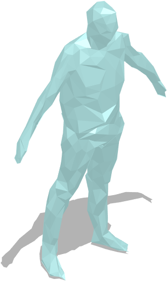
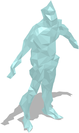
Figure 18: Example of perturbing the geometry on FAUST, with the noise variance set to $0.01$ (left) and $0.02$ (right).

Figure 19: PCK for different amounts of perturbation (Gaussian noise with variance $\sigma^{2}$). We plot our method with solid lines and IsoMuSh [22] with dashed lines. We report results on a class of FAUST.

Appendix L Related Quantum Computer Vision Works

Several quantum methods tackle alignment tasks, as Tab. 5 shows. However, only Q-Match is relevant for comparisons. Several works only consider two point clouds and cannot handle the multi-matching setting of our work, do not consider fully non-rigid transformations, or only operate on point clouds, not meshes. QGM [41] only considers two graphs with at most four vertices. Q-Sync [3] similarly only works on at most five vertices, far fewer than what our method can handle.

Figure 20: We expand the third term of (7) from the main paper, which yields higher-order terms (highlighted in red). When the summands constituting these terms are truly cubic or bi-quadratic, we assume them to be 0, which results in the QUBO (8).

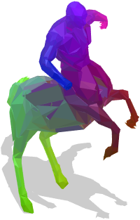
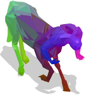
						Ours
Source						IsoMuSh
						ZoomOut
						Q-MatchV2-nc
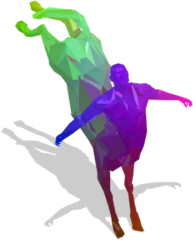
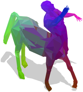
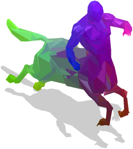
						Q-MatchV2-cc

Figure 22: Qualitative results on the TOSCA [6] centaur class. We colour a source shape and transfer this colouring to target shapes via the matches estimated by our method and competitors.

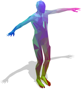
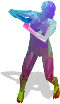
							Ours
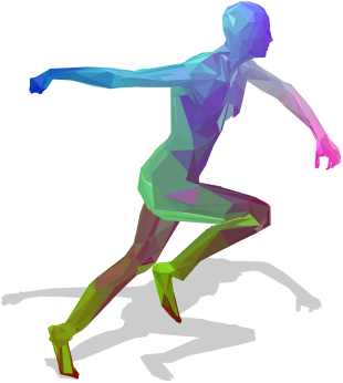
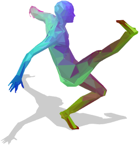
Source							IsoMuSh
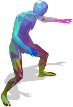
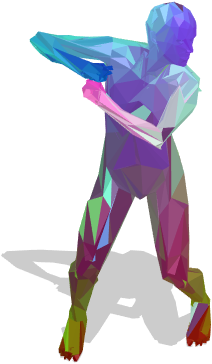
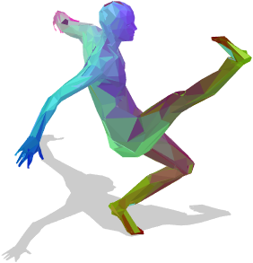
							ZoomOut
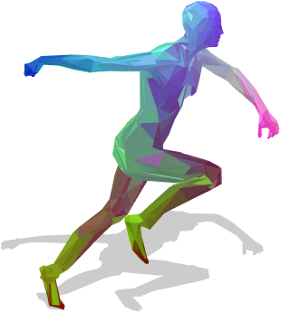
							Q-MatchV2-nc
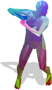
							Q-MatchV2-cc

Figure 23: Qualitative results on the TOSCA [6] David class. We colour a source shape and transfer this colouring to target shapes via the matches estimated by our method and competitors.

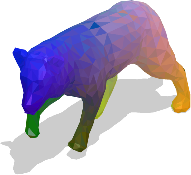
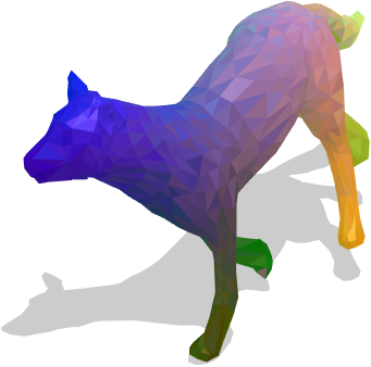
						Ours
Source						IsoMuSh
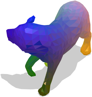
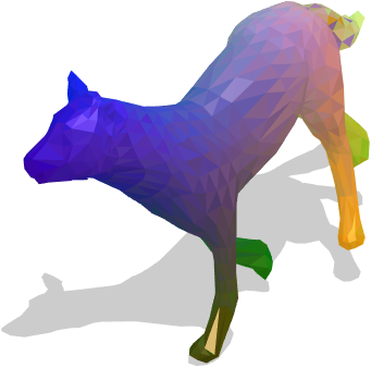
						ZoomOut
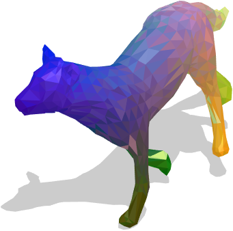
						Q-MatchV2-nc
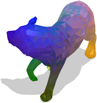
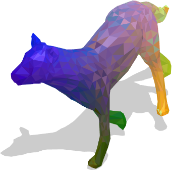
						Q-MatchV2-cc

Figure 24: Qualitative results on a subset of the SMAL dog class. We colour a source shape and transfer this colouring to target shapes via the matches estimated by our method and competitors.

Method	Problem	Transformation	Input Type	# Inputs	# Points	# Qubits (per sweep)	QPU	Iterative
QA, CVPR 2020 [23]	TE, PSR	A/R	point clouds	$2$	${\leq}5k^{\star}$	${\leq}140$	2000Q
IQT, CVPR 2022 [35]	TE	R	point clouds	$2$	${\leq}1.5k^{\star}$	${\leq}10$	2000Q	✓
qKC, ICASSP 2022 [37]	PSR	R	point clouds	$2$	${\leq}2k^{\star}$	$4$-$6$	Rigetti [11]	✓
QGM, 3DV 2020 [41]	GM	F	graphs	$2$	${\leq}4$	${\leq}50$	2000Q
QSync, CVPR 2021 [3]	PS, GM	F	perm. matrices	${\leq}5$	${\leq}5$	$\leq 1.5k$	Adv1.1
QuMoSeg, ECCV 2022 [1]	MS	F	segm. matrices	${\leq}9$	${\leq}200$	$\leq 250$	Adv{1.1;4.1}
Q-Match, ICCV 2021 [42]	MA	R/NR	meshes	$2$	${\leq}500$	${\leq}200$	Adv4.1	✓
CCuantuMM (Ours)	MA	R/NR	meshes	${\leq}100$	${\leq}1k$	${\leq}50$	Adv4.1, Adv2 prototype	✓

Table 5: Overview of related quantum methods for alignment tasks on point sets, graphs and meshes. “^⋆”: according to the experiments reported in the paper; the methods can also process larger point clouds. Key: “TE”: transformation estimation; “PSR”: point set alignment; “GM”: graph matching; “PS”: permutation synchronisation; “MS”: motion segmentation; “MA”: mesh alignment; “A”: affine transformation; “R”: rigid transformation; “NR”: non-rigid deformations; “F”: the method operates on features extracted in a pre-processing step (and can support both rigid and non-rigid transformations). Note that only Q-Match [42] can be extended and applied to our data.

References

- [1] Federica Arrigoni, Willi Menapace, Marcel Seelbach Benkner, Elisa Ricci, and Vladislav Golyanik. Quantum motion segmentation. In Eur. Conf. Comput. Vis., 2022.
- [2] Florian Bernard, Johan Thunberg, Paul Swoboda, and Christian Theobalt. Hippi: Higher-order projected power iterations for scalable multi-matching. In Int. Conf. Comput. Vis., 2019.
- [3] Tolga Birdal, Vladislav Golyanik, Christian Theobalt, and Leonidas Guibas. Quantum permutation synchronization. In IEEE Conf. Comput. Vis. Pattern Recog., 2021.
- [4] Federica Bogo, Javier Romero, Matthew Loper, and Michael J. Black. FAUST: Dataset and evaluation for 3D mesh registration. In IEEE Conf. Comput. Vis. Pattern Recog., 2014.
- [5] Max Born and Vladimir Fock. Beweis des adiabatensatzes. Zeitschrift für Physik, 51(3):165–180, 1928.
- [6] Alexander M Bronstein, Michael M Bronstein, and Ron Kimmel. Numerical geometry of non-rigid shapes. Springer Science & Business Media, 2008.
- [7] Michael M Bronstein and Iasonas Kokkinos. Scale-invariant heat kernel signatures for non-rigid shape recognition. In IEEE Conf. Comput. Vis. Pattern Recog., 2010.
- [8] O. Burghard and R. Klein. Efficient lifted relaxations of the quadratic assignment problem. In Vision, Modeling and Visualization (VMV), 2017.
- [9] Jun Cai, William G Macready, and Aidan Roy. A practical heuristic for finding graph minors. arXiv preprint arXiv:1406.2741, 2014.
- [10] Dongliang Cao and Florian Bernard. Unsupervised deep multi-shape matching. In Eur. Conf. Comput. Vis., 2022.
- [11] Rigetti Computing. https://www.rigetti.com/, 2022.
- [12] Luca Cosmo, Emanuele Rodola, Andrea Albarelli, Facundo Mémoli, and Daniel Cremers. Consistent partial matching of shape collections via sparse modeling. In Computer Graphics Forum, volume 36, pages 209–221. Wiley Online Library, 2017.
- [13] D-Wave. Operation and timing. https://docs.dwavesys.com/docs/latest/c_qpu_timing.html, 2021.
- [14] D-Wave. Zephyr topology of d-wave quantum processors (d-wave technical report series). https://www.dwavesys.com/media/2uznec4s/14-1056a-a_zephyr_topology_of_d-wave_quantum_processors.pdf, 2021.
- [15] D-Wave Systems, Inc. Leap, 2022.
- [16] Nike Dattani. Quadratization in discrete optimization and quantum mechanics. arXiv preprint arXiv:1901.04405, 2019.
- [17] Vasil S Denchev, Sergio Boixo, Sergei V Isakov, Nan Ding, Ryan Babbush, Vadim Smelyanskiy, John Martinis, and Hartmut Neven. What is the computational value of finite-range tunneling? Physical Review X, 6(3):031015, 2016.
- [18] Bailin Deng, Yuxin Yao, Roberto M. Dyke, and Juyong Zhang. A survey of non-rigid 3d registration. Computer Graphics Forum, 41(2):559–589, 2022.
- [19] Theo Deprelle, Thibault Groueix, Matthew Fisher, Vladimir G Kim, Bryan C Russell, and Mathieu Aubry. Learning elementary structures for 3d shape generation and matching. In Neurips, 2019.
- [20] Anh-Dzung Doan, Michele Sasdelli, David Suter, and Tat-Jun Chin. A hybrid quantum-classical algorithm for robust fitting. In IEEE Conf. Comput. Vis. Pattern Recog., 2022.
- [21] Iain Dunning, Swati Gupta, and John Silberholz. What works best when? a systematic evaluation of heuristics for max-cut and qubo. INFORMS Journal on Computing, 30(3):608–624, 2018.
- [22] Maolin Gao, Zorah Lahner, Johan Thunberg, Daniel Cremers, and Florian Bernard. Isometric multi-shape matching. In IEEE Conf. Comput. Vis. Pattern Recog., 2021.
- [23] Vladislav Golyanik and Christian Theobalt. A quantum computational approach to correspondence problems on point sets. In IEEE Conf. Comput. Vis. Pattern Recog., 2020.
- [24] Thibault Groueix, Matthew Fisher, Vladimir G. Kim, Bryan Russell, and Mathieu Aubry. 3d-coded : 3d correspondences by deep deformation. In Eur. Conf. Comput. Vis., 2018.
- [25] Qi-Xing Huang and Leonidas Guibas. Consistent shape maps via semidefinite programming. In Computer graphics forum, volume 32, pages 177–186, 2013.
- [26] Ruqi Huang, Jing Ren, Peter Wonka, and Maks Ovsjanikov. Consistent zoomout: Efficient spectral map synchronization. In Computer Graphics Forum, volume 39, pages 265–278, 2020.
- [27] Lisa Hutschenreiter, Stefan Haller, Lorenz Feineis, Carsten Rother, Dagmar Kainmüller, and Bogdan Savchynskyy. Fusion moves for graph matching. In Int. Conf. Comput. Vis., 2021.
- [28] Itay Kezurer, Shahar Z. Kovalsky, Ronen Basri, and Yaron Lipman. Tight relaxation of quadratic matching. In Symposium on Geometry Processing (SGP), 2015.
- [29] Vladimir G. Kim, Yaron Lipman, and Thomas Funkhouser. Blended intrinsic maps. ACM Trans. Graph., 2011.
- [30] Andrew D King, Jack Raymond, Trevor Lanting, Sergei V Isakov, Masoud Mohseni, Gabriel Poulin-Lamarre, Sara Ejtemaee, William Bernoudy, Isil Ozfidan, Anatoly Yu Smirnov, et al. Scaling advantage over path-integral monte carlo in quantum simulation of geometrically frustrated magnets. Nature communications, 12(1):1–6, 2021.
- [31] Gary Kochenberger, Jin-Kao Hao, Fred Glover, Mark Lewis, Zhipeng Lü, Haibo Wang, and Yang Wang. The unconstrained binary quadratic programming problem: a survey. Journal of combinatorial optimization, 28(1):58–81, 2014.
- [32] Junde Li and Swaroop Ghosh. Quantum-soft qubo suppression for accurate object detection. In Eur. Conf. Comput. Vis., 2020.
- [33] Eleonora Maset, Federica Arrigoni, and Andrea Fusiello. Practical and efficient multi-view matching. In Int. Conf. Comput. Vis., 2017.
- [34] Catherine C. McGeoch. Adiabatic quantum computation and quantum annealing: Theory and practice. Synthesis Lectures on Quantum Computing, 5(2):1–93, 2014.
- [35] Natacha Kuete Meli, Florian Mannel, and Jan Lellmann. An iterative quantum approach for transformation estimation from point sets. In IEEE Conf. Comput. Vis. Pattern Recog., 2022.
- [36] Simone Melzi, Jing Ren, Emanuele Rodola, Abhishek Sharma, Peter Wonka, and Maks Ovsjanikov. Zoomout: Spectral upsampling for efficient shape correspondence. ACM Transactions on Graphics (Proc. SIGGRAPH Asia), 2019.
- [37] Mohammadreza Noormandipour and Hanchen Wang. Matching point sets with quantum circuit learning. In International Conference on Acoustics, Speech and Signal Processing, 2022.
- [38] Deepti Pachauri, Risi Kondor, and Vikas Singh. Solving the multi-way matching problem by permutation synchronization. Adv. Neural Inform. Process. Syst., 2013.
- [39] Yusuf Sahilioglu and Yücel Yemez. Multiple shape correspondence by dynamic programming. Computer Graphics Forum (CGF), 33(7), 2014.
- [40] Yusuf Sahillioglu. Recent advances in shape correspondence. The Visual Computer, 36, 2020.
- [41] Marcel Seelbach Benkner, Vladislav Golyanik, Christian Theobalt, and Michael Moeller. Adiabatic quantum graph matching with permutation matrix constraints. In Int. Conf. 3D Vis. (3DV), 2020.
- [42] Marcel Seelbach Benkner, Zorah Lähner, Vladislav Golyanik, Christof Wunderlich, Christian Theobalt, and Michael Moeller. Q-match: Iterative shape matching via quantum annealing. In Int. Conf. Comput. Vis., 2021.
- [43] Yanyao Shen, Qixing Huang, Nati Srebro, and Sujay Sanghavi. Normalized spectral map synchronization. Adv. Neural Inform. Process. Syst., 2016.
- [44] Ramana Sundararaman, Gautam Pai, and Maks Ovsjanikov. Implicit field supervision for robust non-rigid shape matching. In Eur. Conf. Comput. Vis., 2022.
- [45] Peter JM Van Laarhoven and Emile HL Aarts. Simulated annealing. In Simulated annealing: Theory and applications, pages 7–15. Springer, 1987.
- [46] Matthias Vestner, Zorah Lähner, Amit Boyarski, Or Litany, Ron Slossberg, Tal Remez, Emanuele Rodolà, Alex M. Bronstein, Michael M. Bronstein, Ron Kimmel, and Daniel Cremers. Efficient deformable shape correspondence via kernel matching. In Int. Conf. 3D Vis. (3DV), 2017.
- [47] Jan-Nico Zaech, Alexander Liniger, Martin Danelljan, Dengxin Dai, and Luc Van Gool. Adiabatic quantum computing for multi object tracking. In IEEE Conf. Comput. Vis. Pattern Recog., 2022.
- [48] Silvia Zuffi, Angjoo Kanazawa, David Jacobs, and Michael J. Black. 3D menagerie: Modeling the 3D shape and pose of animals. In IEEE Conf. Comput. Vis. Pattern Recog., 2017.