KeyMatchNet: Zero-Shot Pose Estimation in 3D Point Clouds by Generalized Keypoint Matching

Abstract

In this paper, we present KeyMatchNet, a novel network for zero-shot pose estimation in 3D point clouds. The network is trained to match object keypoints with scene-points, and these matches are then used for pose estimation. The method generalizes to new objects by using not only the scene point cloud as input but also the object point cloud. This is in contrast with conventional methods where object features are stored in network weights. By having a generalized network we avoid the need for training new models for novel objects, thus significantly decreasing the computational requirements of the method.

However, as a result of the complexity, zero-shot pose estimation methods generally have lower performance than networks trained for a single object. To address this, we reduce the complexity of the task by including the scenario information during training. This is generally not feasible as collecting real data for new tasks increases the cost drastically. But, in the zero-shot pose estimation task, no retraining is needed for new objects. The expensive data collection can thus be performed once, and the scenario information is retained in the network weights.

The network is trained on 1,500 objects and is tested on unseen objects. We demonstrate that the trained network can accurately estimate poses for novel objects and demonstrate the ability of the network to perform outside of the trained class. We believe that the presented method is valuable for many real-world scenarios. Code, trained network, and dataset will be made available at publication.

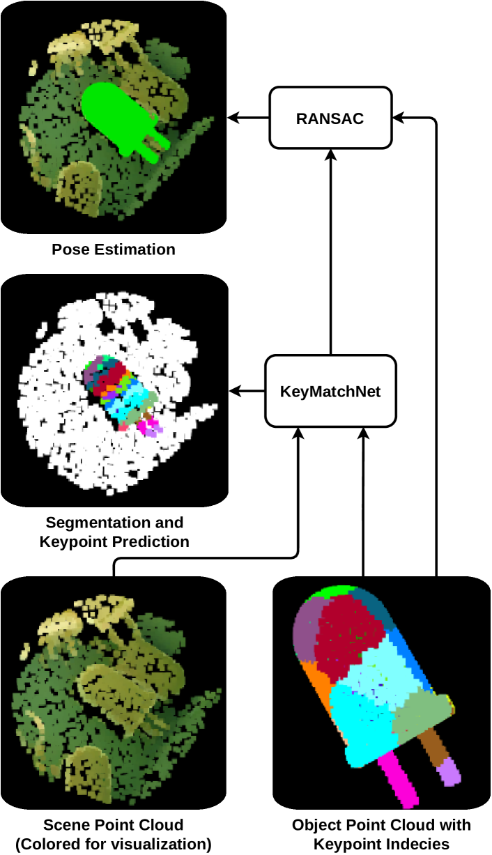
Figure 1: Illustration of the pose estimation method. The input to the network is a scene point cloud and an object point cloud with keypoints spread evenly over the object. The network output is both instance segmentation and keypoint predictions, which are combined to provide predictions only for the object. Finally these predictions are used in RANSAC for pose estimation. The striped keypoint prediction pattern is the result of the objects’ rotational symmetry.

I Introduction

Pose estimation enables greater flexibility in robotics as new objects can be manipulated without the need for mechanical fixtures or teaching specific robot positions. This enables shorter changeover times and faster adaptation to production demands. However, the set-up of computer vision algorithms can itself be a very time-consuming task [1]. There is, therefore, great interest in pose estimation solutions with simple set-ups. Deep learning has allowed learning the specifics of the object and the scenario, thus giving much better performance than human fine-tuning [2, 3]. However, collecting the data for training the deep neural networks can be very time-consuming, limiting the usability. To avoid this data collection, synthetic data has gained widespread use [2]. But generating large amounts of data, and then training the networks for each new object is computationally expensive and increases set-up time. To address these problems, we introduce KeyMatchNet, a neural network built on the principles of reusability. The reusability consists of two parts. Firstly, rather than training a single model for each object, a zero-shot pose estimation algorithm is built. Instead of learning specific features from the object, the network is trained to match keypoints from the object to the scene. Thus, the network input is both scene and object information. For a novel object, the network can be reused without re-training. Additionally, compared with similar methods [4] our network is split into parallel computation of object- and scene-features. This allows for pre-computing the object features, giving a significant speed-up at run-time. Additionally, if multiple objects are pose estimated the scene feature can be reused.

Zero-shot pose estimation methods are, generally, less accurate compared with methods trained for specific objects [5], as they integrate object information into the model. However, these methods use synthetic data and therefore do not integrate scene information. As our model is reused for multiple objects, we can use real data and integrate scene information into the network. For many set-ups this much better fits the tasks at hand. New objects can be introduced faster as training is not required, and the power consumption for training will be removed. An example is robotic work-cells where the set-up is permanent while new objects are often introduced. In this paper we focus on the task of bin picking with homogeneous bins, which is a difficult challenge that often occurs in industry [6]. The homogeneous bin also removes the need for object detection and allows us to only focus on pose estimation. We recognize that the current approach as shown in e.g., [3] has huge importance, but also state it is not the best solution for all tasks. In this paper we show that generalized pose estimation can obtain very good performance when restricting the scenario. We believe that these results invite further research into this topic, as creating flexible set-ups with lower power consumption is an important topic.

II Related Works

As visual pose estimation allow for much more flexible solutions, a large number of different approaches have been developed.

II-A Classic Pose Estimation

In the classic pose estimation case two different approaches are generally used, template matching and feature matching. Template matching [7, 8] is performed using a cascade search of images of the object. To perform the search, images have to be generated of all poses that the object can appear in.

In feature matching pose estimation is based on matching features between the scene and object, and computing the pose by e.g. RANSAC [9]. The matches are computed using handcrafted features, which is generally computed in 3D point clouds. A huge amount of handcrafted features have been developed [10], with Fast Point Feature Histograms (FPFH) [11] being one of the best performing features. The benefit of the classic methods is the set-up does not , weak towards clutter and occlusion.

II-B Deep Learning Based

Generally deep learning based methods are based on color information [2, 3]. This is possibly a result of many deep learning based methods developed for this space, with huge pre-trained networks available. These methods have vastly outperformed the classical methods, however, a network is often trained per object [2, 3]. Deep learning for pose estimation has also been performed in point clouds with methods such as PointVoteNet [12]. We base our method on PointVoteNet, but only train a single network for all objects.

2D methods: SSD-6D [13] is similar to template matching methods, in that it employs the cascade search. However, unlike template matching the comparison is performed using a neural network. The network is trained to classify the presence and correct orientation of an object. Thus by cascade search in the image the correct object pose is found. The position and orientation can also be computed independently [14, 15]. In PoseCNN [14] the orientation is computed using a regression network.

An alternate approach is by detecting keypoints of the object [16, 15]. This is performed in BB-8 [17] where the bounding box is predicted and then used for pose estimation. PVNet [18] compute keypoint locations by first segmentation the object, and then computing the relative position of keypoint for all pixels belonging to the object.

A method more similar to our approach is EPOS [19] where both object segmentation and dense keypoint predictions are calculated. This approach is also performed in DPOD [20] which also employs pose refinement. Unlike our methods these methods use RGB information and train a single network per object.

3D methods: DenseFusion [21] is a method that combines both 2D and 3D information. Initial segmentations are found in 2D, and features computed in 2D are then integrated with 3D features. The 3D features are computed using PointNet [22]. Finally a PnP is used to perform pose estimation using keypoints from the network. PVN3D [23] is another method that combines 2D and 3D features. It also computes keypoints for which are used for pose estimation. Unlike our method the keypoints are the object bounding box, and not keypoints on the object.

A method more similar to our method is PointVoteNet [12]. Here PointNet [22] is used to compute keypoints for each scene point. Similar to our method the computation is also performed without color information. In the extended version [24] DGCNN [25] is used and the segmentation and feature computation is separated, both of which appears in our method. However, dissimilar to our method, for PointVoteNet a network is trained for each object.

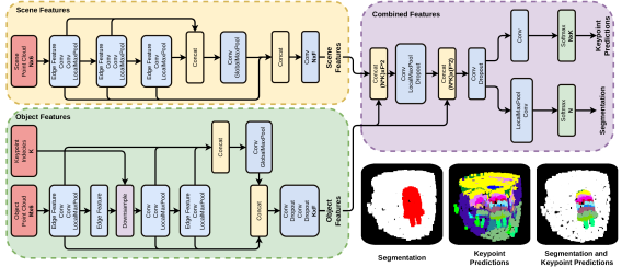
Figure 2: The network structure of the developed method. Object and scene features are initially computed independently. This allows us to compute the object feature once and match it to multiple scene point clouds. The Segmentation and Keypoint Prediction outputs are shown along with the combination. It is seen that the Keypoint Predictions are calculated for both objects in the scene and the instance segmentation filters out the other object.

II-C Generalized Pose Estimation

Several approaches have been developed for generalized pose estimation. As in the deep learning based pose estimation, the field of generalized pose estimation is also dominated by color-based methods [26, 5, 27]. The general approach for these methods is to match templates of the object with the real image, similar to SSD-6D. These templates can either be generated synthetically as in [28] or with a few real images as in FS6D [27]. The same approach have also been used for tracking of unknown objects [29]. As opposed to SSD-6D the network does not learn to recognize specific poses of objects, but instead to compare how well an image match the real scene. By generating synthetic views of novel objects, these methods are thus able to perform pose estimation without training new networks. MegaPose6D [5] is a notable example where the network is trained on a huge dataset with 2 million images.

The method most similar to ours is a point cloud based method [4]. It also uses the object point cloud as input along with the scene point cloud. The method also employs a segmentation step as in our method, however the pose estimation part of the method whereas our approach matches specific keypoint. Several other differences are also present compared with our approach; the method includes color information which is often much more difficult to obtain. It does not limit the scenario and thus does not obtain the increased performance from this. And it does not separate the object and scene features, thus the object features must be computed for each pose estimation.

III Method

The developed method is a network that matches scene-points to object keypoints. These matches are then feed into a pose estimation solver, in our case RANSAC, and a final pose is found. The scene and object data are point clouds without color information. Color information is not used as it is seldom available for CAD (Computer Aided Design) models and would limit the usability of the method. The network structure is made with two parallel components computing both scene- and object-features independently. The network structure is shown in Fig. 2. The scene features are computed for all points using the standard DGCNN [30]. However, for the object only the keypoint features are computed. Thus, after the second neighbor computation the object features are down-sampled to only contain the keypoints. For the object-feature computation, number of neighbors is set to the number of keypoints, ensuring that the keypoints share all information.

After both object- and scene-features are computed, the features are combined. Pairs of object- and scene-feature vectors are created concatenating each scene-feature with each object-feature. The resulting number of pairs is the number of scene-points and key-points multiplied. An MLP (Multi Layer Perceptron) then processes each scene-keypoint pair independently and a local maxpool combines all keypoint information at the scene point.

This new scene feature is again combined with the keypoint features, and processed by an MLP. Two different MLPs are then used to compute the segmentation and the keypoint predictions. To compute the segmentation a local maxpool is applied followed by an MLP which gives segmentation for each point. To compute the keypoint matches an MLP is applied to the combined features giving a score for each scene-keypoint pair. A softmax is then applied across the keypoint domain for each scene point, predicting the best scene-keypoint match. Finally, RANSAC is used with the segmentation and keypoint predictions to compute the final object pose. We employ the vote threshold as in [12] to allow multiple keypoint matches at a single scene point. The vote threshold is set to 0.7.

III-A GPU based RANSAC:

To compare the classic pose estimation method and our developed method a classic RANSAC is implemented using Open3D [31]. However, as the RANSAC method is running on the CPU a significant increase in run-time occurs. To decrease the run-time a RANSAC has also been implemented on the GPU using PyTorch [32].

The GPU based RANSAC is implemented as a Coarse-to-Fine RANSAC, with five iterations. Initially, 1000 poses are computed using the Kabsch [33] algorithm on triplets sampled from the matches. The poses are then sorted according to the amount of inliers based on matches. And additional requirement is that the normal vector between matches cannot be higher than 30 degrees. This is to ensure that the backside of models are not matched.

The best scoring pose is then selected, and further refinement is performed. The pose is refined by computing the Kabsch using only matches within the inlier distance. Further refinement is obtained by gradually decreasing the inlier distance. The distance is decreased by dividing by 2, 3, 4 and 5. As the RANSAC includes refinement, ICP is not used for the GPU based RANSAC.

III-B Generating object data:

The object point clouds is generated using Poisson sampling to obtain 2048 evenly sampled points on the surface. Farthest point sampling is then used to obtain the keypoints spread evenly on the object.

III-C Computing object features off-line:

As shown in Fig. 2 the features computed from the object point cloud are independent of the features computed from the scene point cloud. This is opposed to [4]. This allow us to use the same object feature for multiple pose estimations. The object features can also be computed offline to reduce the run-time and the computational cost. During training the keypoints are continuously re-computed with random initialization, to avoid the network over-fitting to a specific combination.

III-D Generating scene data:

The scene point clouds are generated using BlenderBin. BlenderBin is an open-source tool built using the BlenderProc [34] simulator. It allows to easily generate synthetic data with objects placed in bins. For each object images are created with the number of objects in the bin ranging from one to twenty. The bin model is kept the same in all scenes. Examples of the training data is shown in Fig. 3.

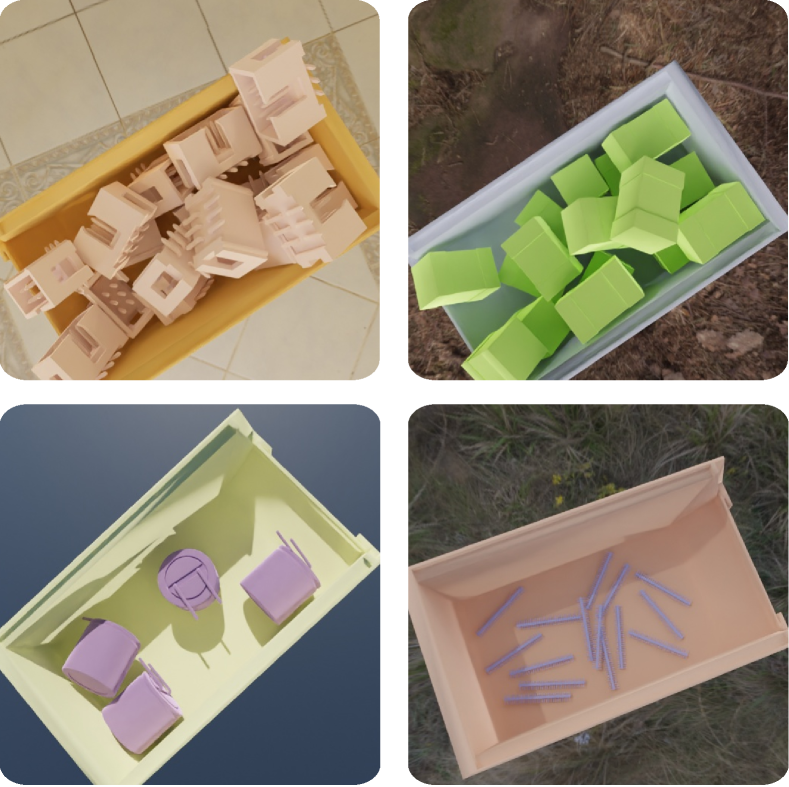
Figure 3: Examples from the training data. The colors are only for visualization.

As the scenario is homogeneous bin-picking the detection is vastly simplified. By segmenting the known bin, all remaining points belong to objects. As the contents are homogeneous any random point is known to belong to a correct object. By then extracting a point cloud around the sampled point using the object diagonal, all points in the scene belonging to the object will be obtained. The point cloud is then centered around the sampled point to allow for instance segmentation.

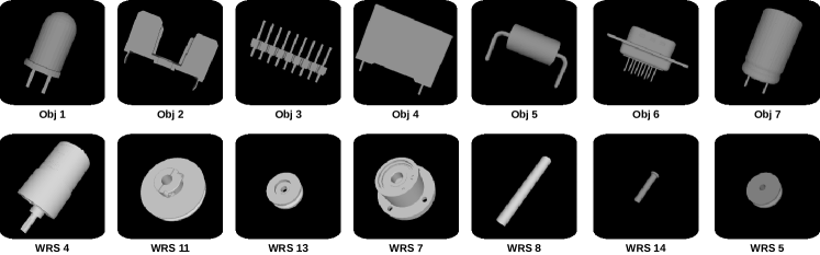
Figure 4: The seven electronic components used for testing, along with the seven components from the WRS dataset used for out of class testing.

IV Experiments

To test the developed method several experiments are performed. A single model is trained, and used for all experiments. The training data consists of 1,500 CAD models of electric components introduced in [35]. Fifty models excluded from the training to test the networks pose estimation ability on unseen objects.

Additionally we test the ability of the network on out of class objects. Seven industrial objects from the WRS [6] dataset is used for testing. On this dataset we show the networks ability to generalize to other objects outside of the training scope. All point cloud processing and pose estimation is performed using the Open3D framework, [31]. The network processing was performed using PyTorch [32].

IV-A Network Training

The network was trained on a PC environment with two NVIDIA GeForce RTX 2080 GPUs. The network was trained for 120 epochs lasting approximately six days (141 hours). For each object we generate 160 point clouds giving an epoch size of 232,000.

The network is trained with a batch size of 14, with 7 on each GPU, using the Adam optimizer [36], with an initial learning rate of 0.0001. We use a step scheduler with a step size of 20 and the gamma parameter set to 0.7. The loss is calculated with cross entropy using a 0.2/0.8 split for segmentation and keypoint loss. For the keypoint loss only points belonging to the object is used. Group norm [37] with size 32 is used as opposed to Batch Norm as a result of the small batch size.

Dropout is applied after the object features, as the network should not overfit to a specific part of the object, and is used after the to concurrent linear layers. The dropout is set to 40 %, used after the last two linear layers of the object feature and the first two of the combined feature. Additionally, up to 0.7 % Gaussian noise is applied to the object and scene point clouds, and 10 % position shift is applied to the object point cloud.

IV-B Training and test performance

The performance for the trained networks is show in Tab. I. Performance is shown for both the loss, segmentation accuracy, and keypoint accuracy. We present the performance on the training data both with and without generalization. The network does not appear to overfit to the training data, and actually shows better performance on the test set. As the objects are symmetric to varying levels, the keypoint accuracy despite being low, still gives good pose estimations. This is seen in Fig. 1, where the symmetry of the object results in striped matching of keypoints. However, these matches are still very useful for the pose estimation. This is further shown in Fig. 5.

TABLE I: The loss and accuracy of the network on the different datasets. Results are shown for the training data both with and without the generalization applied during training.

Split	Train (w/ gen.)	Train (w/o gen.)	Test
Loss	1.59	1.42	1.33
Seg. Acc	0.98	0.97	0.96
Key. Acc	0.27	0.29	0.31

To analyze the network, performance for each component is shown in Tab. II. The two objects with the highest smallest loss is ”3” and ”5”. These two object are both very similar to objects in the training data. The most challenging object is ”2”. The split between the two parts of the object makes it very dissimilar to the training data. The other components perform very well, especially for the segmentation task.

TABLE II: Loss and accuracy of each of the individual test objects.

Object	1	2	3	4	5	6	7
Loss	1.50	2.03	1.12	1.53	1.42	1.84	1.53
Seg. Acc	0.99	0.81	0.98	0.98	0.95	0.97	0.99
Key. Acc	0.24	0.16	0.43	0.29	0.31	0.22	0.22

IV-C Pose Estimation Performance

To test the pose estimation accuracy of the developed method we compare it with the classic pose estimation method FPFH [11]. For both methods, RANSAC is used [9]. Additionally, we test our method using the GPU based RANSAC. The performance is measured by the ADI score, as it is well suited for the symmetric objects in the dataset. The classic method obtains a $0.57\%$ mean accuracy whereas our method obtains a $0.95\%$ mean accuracy. Using the GPU based RANSAC the mean accuracy is $0.86\%$. A slightly lower performance. Our method thus vastly outperforms the classic pose estimation method.

To further test the robustness of the system, varying levels of noise is added to the points clouds. The results are shown in Tab. III. It can be seen that our method outperforms the classic method for all objects. When adding noise the difference becomes even more pronounced. However, for the $5\%$ noise the performance also drops significantly for our method.

TABLE III: Pose estimation accuracy for each of the test components. A comparison with classic pose estimation is shown. Results are also shown with noise added to the scene point cloud.

Object	1	2	3	4	5	6	7
Ours	0.95	0.82	0.99	0.77	0.91	0.90	0.92
Classic	0.55	0.62	0.61	0.30	0.36	0.67	0.51
Ours $1\%$	0.93	0.79	0.99	0.74	0.86	0.88	0.90
Classic $1\%$	0.43	0.57	0.50	0.25	0.31	0.66	0.40
Ours $5\%$	0.55	0.60	0.91	0.62	0.83	0.82	0.53
Classic $5\%$	0.30	0.54	0.45	0.20	0.43	0.56	0.25

TABLE IV: Pose estimation accuracy on the out-of-class dataset. The objects are numbered according to [6]. A comparison with classic pose estimation is shown. Results are also shown with noise added to the scene point cloud.

Number	4	11	13	7	8	14	5
Type	Motor	Pulley	Idler	Bear.	Shaft	Screw	Pulley
Ours	1.00	0.99	0.90	0.91	0.93	0.93	0.96
GPU	1.00	0.99	0.98	0.96	0.90	0.97	0.98
Classic	0.98	0.93	0.78	0.78	0.67	0.37	0.90
Ours $1\%$	1.00	0.99	0.89	0.94	0.93	0.92	0.96
GPU $1\%$	1.00	0.99	0.97	0.97	0.89	0.96	0.98
Cla.  $1\%$	0.95	0.91	0.75	0.79	0.65	0.30	0.89
Ours $5\%$	0.97	0.98	0.87	0.94	0.82	0.73	0.95
GPU $5\%$	0.97	0.97	0.88	0.95	0.67	0.70	0.92
Cla.  $5\%$	0.67	0.89	0.74	0.82	0.57	0.28	0.80

Object        Scene        Prediction     Accuracy Pose Estimation

Figure 5: Visualization of network output and resulting pose estimation using the RANSAC from Open3D [31]. From left to right is shown: object with keypoints, scene point cloud, keypoint prediction, accuracy of keypoint prediction and finally the pose estimation. The pose estimation accuracy is shown as follows: ”White” represents correctly predicted background, ”red” false negatives and ”yellow” false positives. ”Blue” is correctly predicted segmentation of the object, but wrong keypoints and ”green” is both correct segmentation and keypoint prediction. It is seen that segmentation prediction is very high, and while the keypoint accuracy is not very high the pose estimation are correct. The objects are Obj 1, Obj 4, WRS 7 and WRS 4 from top to bottom.

Testing out of class: The out-of-class dataset consists of industrial objects, such as motors and pulleys. The objects were used for the WRS assembly challenge held in 2018 [6]. The objects were chosen as they represent an industrial challenge, and because of the variety. To further test the robustness of the system, varying levels of noise is added to the points clouds.

The results of the network performance and pose estimation is shown in Tab. IV. It is seen that our developed method obtains very good performance on these objects that appear quite different compared with the training data. When adding noise the difference becomes even more pronounced. The ability to correctly compute features for both in and out-of-class objects is shown in Fig. 5. The GPU based method actually shows better performance than the comparison method. However, these is a noticeable drop for object id 8 with 5 % noise.

IV-D Run-time

The run-time of the network was tested both with and without computing the object features at run-time. With the object features computed at run-time the processing lasts 14.9 ms. While by pre-computing the features the run-time is only 7.9 ms. The separation of object and scene feature computations is thus a significant speed-up.

However, for the full system the run-time is currently 84.7 ms. This is mainly related to the RANSAC which is computed on the CPU using Open3D [31]. By running the RANSAC using the GPU the run-time using pre-computed object features is reduced to 19.9 ms. A significant speed-up is thus obtained with a speed of 50 frames per second.

V Conclusion

This paper presents a novel method for zero-shot pose estimation. The main contributions of the paper is a novel network structure with independent object and scene feature computation, and a scenario-specific approach. This method shows very good generalizability across different objects, including out-of-class objects. This proves the validity of creating object independent networks for specific scenarios, which can be useful for many real world applications.

In future work, it will be very interesting to test the method with real data, both for training and testing. Additionally, the network could be adapted to perform full pose estimation to simplify the pipeline and improve the run-time. The objects from the MegaPose6D [5] dataset could also be used to diversify the object types, and test on benchmark datasets.

References

- [1] F. Hagelskjær, A. G. Buch, and N. Krüger, “Does vision work well enough for industry?” in VISIGRAPP (4: VISAPP), 2018, pp. 198–205.
- [2] T. Hodaň, M. Sundermeyer, B. Drost, Y. Labbé, E. Brachmann, F. Michel, C. Rother, and J. Matas, “Bop challenge 2020 on 6d object localization,” in Computer Vision–ECCV 2020 Workshops: Glasgow, UK, August 23–28, 2020, Proceedings, Part II 16. Springer, 2020, pp. 577–594.
- [3] M. Sundermeyer, T. Hodan, Y. Labbe, G. Wang, E. Brachmann, B. Drost, C. Rother, and J. Matas, “Bop challenge 2022 on detection, segmentation and pose estimation of specific rigid objects,” arXiv preprint arXiv:2302.13075, 2023.
- [4] M. Gou, H. Pan, H.-S. Fang, Z. Liu, C. Lu, and P. Tan, “Unseen object 6d pose estimation: a benchmark and baselines,” arXiv preprint arXiv:2206.11808, 2022.
- [5] Y. Labbé, L. Manuelli, A. Mousavian, S. Tyree, S. Birchfield, J. Tremblay, J. Carpentier, M. Aubry, D. Fox, and J. Sivic, “Megapose: 6d pose estimation of novel objects via render & compare,” arXiv preprint arXiv:2212.06870, 2022.
- [6] Y. Yokokohji, Y. Kawai, M. Shibata, Y. Aiyama, S. Kotosaka, W. Uemura, A. Noda, H. Dobashi, T. Sakaguchi, and K. Yokoi, “Assembly challenge: a robot competition of the industrial robotics category, world robot summit–summary of the pre-competition in 2018,” Advanced Robotics, vol. 33, no. 17, pp. 876–899, 2019.
- [7] M. Ulrich, C. Wiedemann, and C. Steger, “Combining scale-space and similarity-based aspect graphs for fast 3d object recognition,” IEEE transactions on pattern analysis and machine intelligence, vol. 34, no. 10, pp. 1902–1914, 2012.
- [8] S. Hinterstoisser, V. Lepetit, S. Ilic, S. Holzer, G. Bradski, K. Konolige, and N. Navab, “Model based training, detection and pose estimation of texture-less 3d objects in heavily cluttered scenes,” in Asian conference on computer vision. Springer, 2012, pp. 548–562.
- [9] M. A. Fischler and R. C. Bolles, “Random sample consensus: a paradigm for model fitting with applications to image analysis and automated cartography,” Communications of the ACM, vol. 24, no. 6, pp. 381–395, 1981.
- [10] Y. Guo, M. Bennamoun, F. Sohel, M. Lu, J. Wan, and N. M. Kwok, “A comprehensive performance evaluation of 3d local feature descriptors,” International Journal of Computer Vision, vol. 116, pp. 66–89, 2016.
- [11] R. B. Rusu, N. Blodow, and M. Beetz, “Fast point feature histograms (fpfh) for 3d registration,” in 2009 IEEE international conference on robotics and automation. IEEE, 2009, pp. 3212–3217.
- [12] F. Hagelskjær and A. G. Buch, “Pointvotenet: Accurate object detection and 6 dof pose estimation in point clouds,” in 2020 IEEE International Conference on Image Processing (ICIP). IEEE, 2020, pp. 2641–2645.
- [13] W. Kehl, F. Manhardt, F. Tombari, S. Ilic, and N. Navab, “Ssd-6d: Making rgb-based 3d detection and 6d pose estimation great again,” in IEEE International Conference on Computer Vision, 2017, pp. 1521–1529.
- [14] Y. Xiang, T. Schmidt, V. Narayanan, and D. Fox, “Posecnn: A convolutional neural network for 6d object pose estimation in cluttered scenes,” Robotics: Science and Systems, 2018.
- [15] Z. Li, G. Wang, and X. Ji, “Cdpn: Coordinates-based disentangled pose network for real-time rgb-based 6-dof object pose estimation,” in Proceedings of the IEEE International Conference on Computer Vision, 2019, pp. 7678–7687.
- [16] B. Tekin, S. N. Sinha, and P. Fua, “Real-time seamless single shot 6d object pose prediction,” in Proceedings of the IEEE Conference on Computer Vision and Pattern Recognition, 2018, pp. 292–301.
- [17] M. Rad and V. Lepetit, “Bb8: A scalable, accurate, robust to partial occlusion method for predicting the 3d poses of challenging objects without using depth,” in IEEE International Conference on Computer Vision, 2017, pp. 3828–3836.
- [18] S. Peng, Y. Liu, Q. Huang, X. Zhou, and H. Bao, “Pvnet: Pixel-wise voting network for 6dof pose estimation,” in IEEE Conference on Computer Vision and Pattern Recognition, 2019, pp. 4561–4570.
- [19] T. Hodan, D. Barath, and J. Matas, “Epos: Estimating 6d pose of objects with symmetries,” in Proceedings of the IEEE/CVF Conference on Computer Vision and Pattern Recognition, 2020, pp. 11 703–11 712.
- [20] S. Zakharov, I. Shugurov, and S. Ilic, “Dpod: 6d pose object detector and refiner,” in Proceedings of the IEEE International Conference on Computer Vision, 2019, pp. 1941–1950.
- [21] C. Wang, D. Xu, Y. Zhu, R. Martín-Martín, C. Lu, L. Fei-Fei, and S. Savarese, “Densefusion: 6d object pose estimation by iterative dense fusion,” in IEEE Conference on Computer Vision and Pattern Recognition, 2019, pp. 3343–3352.
- [22] C. R. Qi, H. Su, K. Mo, and L. J. Guibas, “Pointnet: Deep learning on point sets for 3d classification and segmentation,” in IEEE Conference on Computer Vision and Pattern Recognition, 2017, pp. 652–660.
- [23] Y. He, W. Sun, H. Huang, J. Liu, H. Fan, and J. Sun, “Pvn3d: A deep point-wise 3d keypoints voting network for 6dof pose estimation,” in Proceedings of the IEEE/CVF conference on computer vision and pattern recognition, 2020, pp. 11 632–11 641.
- [24] F. Hagelskjær and A. G. Buch, “Bridging the reality gap for pose estimation networks using sensor-based domain randomization,” in Proceedings of the IEEE/CVF International Conference on Computer Vision, 2021, pp. 935–944.
- [25] Y. Wang, Y. Sun, Z. Liu, S. E. Sarma, M. M. Bronstein, and J. M. Solomon, “Dynamic graph cnn for learning on point clouds,” ACM Transactions on Graphics, 2019.
- [26] I. Shugurov, F. Li, B. Busam, and S. Ilic, “Osop: a multi-stage one shot object pose estimation framework,” in Proceedings of the IEEE/CVF Conference on Computer Vision and Pattern Recognition, 2022, pp. 6835–6844.
- [27] Y. He, Y. Wang, H. Fan, J. Sun, and Q. Chen, “Fs6d: Few-shot 6d pose estimation of novel objects,” in Proceedings of the IEEE/CVF Conference on Computer Vision and Pattern Recognition, 2022, pp. 6814–6824.
- [28] V. N. Nguyen, Y. Hu, Y. Xiao, M. Salzmann, and V. Lepetit, “Templates for 3d object pose estimation revisited: generalization to new objects and robustness to occlusions,” in Proceedings of the IEEE/CVF Conference on Computer Vision and Pattern Recognition, 2022, pp. 6771–6780.
- [29] V. N. Nguyen, Y. Du, Y. Xiao, M. Ramamonjisoa, and V. Lepetit, “Pizza: A powerful image-only zero-shot zero-cad approach to 6 dof tracking,” arXiv preprint arXiv:2209.07589, 2022.
- [30] Y. Wang, Y. Sun, Z. Liu, S. E. Sarma, M. M. Bronstein, and J. M. Solomon, “Dynamic graph cnn for learning on point clouds,” Acm Transactions On Graphics (tog), vol. 38, no. 5, pp. 1–12, 2019.
- [31] Q.-Y. Zhou, J. Park, and V. Koltun, “Open3D: A modern library for 3D data processing,” arXiv:1801.09847, 2018.
- [32] A. Paszke, S. Gross, F. Massa, A. Lerer, J. Bradbury, G. Chanan, T. Killeen, Z. Lin, N. Gimelshein, L. Antiga, A. Desmaison, A. Kopf, E. Yang, Z. DeVito, M. Raison, A. Tejani, S. Chilamkurthy, B. Steiner, L. Fang, J. Bai, and S. Chintala, “PyTorch: An Imperative Style, High-Performance Deep Learning Library,” in Advances in Neural Information Processing Systems 32, H. Wallach, H. Larochelle, A. Beygelzimer, F. d’Alché Buc, E. Fox, and R. Garnett, Eds. Curran Associates, Inc., 2019, pp. 8024–8035.
- [33] W. Kabsch, “A solution for the best rotation to relate two sets of vectors,” Acta Crystallographica Section A: Crystal Physics, Diffraction, Theoretical and General Crystallography, vol. 32, no. 5, pp. 922–923, 1976.
- [34] M. Denninger, M. Sundermeyer, D. Winkelbauer, Y. Zidan, D. Olefir, M. Elbadrawy, A. Lodhi, and H. Katam, “Blenderproc,” arXiv preprint arXiv:1911.01911, 2019.
- [35] F. Hagelskjær and D. Kraft, “In-hand pose estimation and pin inspection for insertion of through-hole components,” in 2022 IEEE 18th International Conference on Automation Science and Engineering (CASE). IEEE, 2022, pp. 382–389.
- [36] D. P. Kingma and J. Ba, “Adam: A method for stochastic optimization,” arXiv preprint arXiv:1412.6980, 2014.
- [37] Y. Wu and K. He, “Group normalization,” in Proceedings of the European conference on computer vision (ECCV), 2018, pp. 3–19.