Two-step estimation of latent trait models

Abstract

We consider two-step estimation of latent variable models, in which just the measurement model is estimated in the first step and the measurement parameters are then fixed at their estimated values in the second step where the structural model is estimated. We show how this approach can be implemented for latent trait models (item response theory models) where the latent variables are continuous and their measurement indicators are categorical variables. The properties of two-step estimators are examined using simulation studies and applied examples. They perform well, and have attractive practical and conceptual properties compared to the alternative one-step and three-step approaches. These results are in line with previous findings for other families of latent variable models. This provides strong evidence that two-step estimation is a flexible and useful general method of estimation for different types of latent variable models.

Key words: Item response theory models; latent variable models; structural equation models; pseudo-maximum likelihood estimation

1 Introduction

Latent variable models have normally two distinct parts: a measurement model which describes how the latent variables that appear in the model are measured by observed indicators of them, and a structural model which describes the associations among the latent variables and any observed explanatory and response variables which are not treated as measurement indicators. For instance, in the illustrative example considered in Section 5 of this paper the structural model specifies how individuals’ extrinsic and intrinsic work value orientations are associated with characteristics of the individuals, and the measurement model how these value orientations are measured by a set of survey questions. Here, as in many applications, the structural model is the focus of substantive interest, but the measurement model also needs to be included and estimated in order for the structural model to be estimable.

Estimation of these elements can be organised in different ways. In joint or one-step estimation, both parts of the model are estimated together. When this is done by maximizing the joint likelihood, one-step estimates are the maximum likelihood (ML) estimates of the model parameters. In contrast, “stepwise” approaches divide the estimation of the two parts into separate steps. The most familiar of them is three-step estimation. In its first step, the measurement model is estimated from the simplest specification that allows this, omitting all or most of the structural model. In the second step, this estimated measurement model is used to assign predicted values of the latent variables to the units of analysis, such as factor scores for continuous latent variables. In the third step, these values are used in place of the latent variables to estimate the structural model. There are “naive” and “adjusted” versions of three-step estimation, depending on whether it attempts to account for the measurement error that results from using the predicted values (this will be discussed further in Section 3.3).

The focus of this paper is on a different stepwise approach, two-step estimation of latent variable models. Its first step is estimation of the measurement model, as in the three-step method. In the second step, instead of being used to calculate explicit predictions for the latent variables, the parameters of the measurement model are simply fixed at their estimated values. In other words, the second step takes the same form as one-step estimation, except that all the measurement parameters are treated as known numbers rather than unknown estimands. Likelihood-based two-step estimation derives its justification and properties from the general theory of pseudo maximum likelihood estimation, as discussed in Section 3.2 below. Its large-sample properties are very similar to those of one-step ML estimation.

Two-step estimates avoid the measurement error bias of naive three-step estimates and are typically comparable in performance, but practically simpler than, adjusted three-step estimates. Compared to one-step estimation, the two-step approach has in principle attractive practical and conceptual advantages. Because it is split into two steps, both of them will be computationally less demanding than the single step of one-step estimation. It is also easy to estimate the measurement and structural models using fully or partially different sets of data, which is necessary in some applications. The conceptual advantage arises from an inherent difference in how the two methods use the available data. Because the one-step approach fits all parts of the model at once, the estimated measurement model is informed not only by the measurement indicators but also by the observed covariates and responses in the structural model. This can cause what Burt (1973, 1976) terms “interpretational confounding”, a situation where the implied definition of a latent variable is in effect partly determined by variables that should be conceptually separate from it. A related problem is that the estimated measurement model will change whenever the structural model is changed, and misspecification of the structural model may also distort the measurement parameters. These risks are naturally avoided by the two-step approach because it estimates the measurement model only once and using only the measurement indicators.

Two-step estimation is a general idea, and one of the points that we want to make in this paper is that it can in principle be applied to any latent variable models. However, there may be differences in performance of the estimates, ease of implementation or other points to consider when it is used for different broad types of models. In the literature so far, two-step estimation has accordingly been described for specific types of models. It was proposed for latent class analysis, that is for models where both the latent variables and their indicators are categorical, by Bandeen-Roche et al. (1997), Xue and Bandeen-Roche (2002) and Bakk and Kuha (2018), and has since been extended to further versions of them (e.g. multilevel latent class analysis in Di Mari et al. 2023). For structural equation models (SEMs), where the latent variables and indicators are both continuous, the idea was introduced already by Burt (1973, 1976), but detailed exploration of it is much more recent. In particular, Rosseel and Loh (2022) proposed a general two-step approach for SEMs, with the title of “structural-after-measurement” (SAM) estimation. They describe two (usually equivalent) forms of it: “local SAM” which summarises the first step in the form of the estimated means and covariance matrix of the variables in the structural model, and “global” SAM which is analogous to the implementation that we describe in this paper for latent trait models (the moment-based “local” approach is not really applicable to them). A method for SEMs is also proposed by Levy (2023), using Bayesian (MCMC) estimation for both steps. Another closely related paper is Skrondal and Kuha (2012), who use two-step estimation to correct for covariate measurement error in regression models. Two-step methods for these classes of models are now also being implemented in general-purpose software for latent variable modelling, in Latent Gold for latent class analysis (Vermunt and Magidson, 2021b) and the R package lavaan for SAM (Rosseel, 2012; Rosseel and Loh, 2022).

In this paper we propose and examine two-step estimation for another family of latent variable models, one where the latent variables are continuous but their indicators are categorical (in our presentation they are all dichotomous for simplicity, but the extension to polytomous items is immediate). These are commonly known as Item Response Theory (IRT) models. Here we refer to them also as latent trait models. They resemble SEMs in having continuous latent variables, and latent class models in having categorical indicators. Like SEMs, they are often used with complex structural models which include multiple latent variables, whereas latent class analysis more often includes only one latent class variable. Computationally, latent trait models are typically the most demanding of these families of models, because their log likelihood cannot be expressed in a closed form.

We describe the theory and implementation of two-step estimation of latent trait models. The presentation of this broadly parallels that of Bakk and Kuha (2018) for latent class models, but with the changes that are needed now that the latent variables are continuous. We then use simulation studies and an application example to explore the properties of the method in this context. Here one question of interest is whether its relative performance is similar to what it is for previously considered types of models. The conclusion is that it is, with some differences of emphasis (these findings are discussed in more detail in Sections 4–6). Two-step estimates of the structural model again perform very well compared to both one-step and (naive) three-step estimates. In complex models their computational advantage compared to one-step estimation can be even larger than for latent class models and SEMs. On the other hand, interpretational confounding of one-step estimates may be less worrying here than for latent class models, because shifts in interpretation tend to be less abrupt for continuous latent variables than for categorical ones.

The latent trait model specifications that we consider are introduced in Section 2. The definition, implementation and properties of two-step estimation for them are described in Section 3. Simulation studies are reported in Section 4 and the real-data example in Section 5, and concluding discussion is given in Section 6. Extended tables of some of the results from the simulations and data analysis are given in a supplementary appendix. [Computer code for the estimation in R and Mplus (both of which are needed) and replication code for the applied example are also provided as supplementary materials.]

2 Models and variables

To begin with a general formulation of a latent variable model, let $\boldsymbol{\eta}_{i}$ be a vector of latent variables, and $\mathbf{Y}_{i}$, $\mathbf{X}_{i}$ and $\mathbf{Z}_{i}$ distinct vectors of observed variables, for a unit of analysis $i$. Consider a model of the form $p(\mathbf{Y}_{i},\boldsymbol{\eta}_{i},\mathbf{Z}_{i}|\mathbf{X}_{i};\boldsymbol{\theta})=p(\mathbf{Y}_{i}|\boldsymbol{\eta}_{i},\mathbf{Z}_{i},\mathbf{X}_{i};\boldsymbol{\theta}_{1})\,\times p(\boldsymbol{\eta}_{i},\mathbf{Z}_{i}|\mathbf{X}_{i};\boldsymbol{\theta}_{2})$, where $p(\cdot|\cdot)$ denotes a conditional distribution and $\boldsymbol{\theta}=(\boldsymbol{\theta}_{1}^{\prime},\boldsymbol{\theta}_{2}^{\prime})^{\prime}$ are parameters. Here $p(\mathbf{Y}_{i}|\boldsymbol{\eta}_{i},\mathbf{Z}_{i},\mathbf{X}_{i};\boldsymbol{\theta}_{1})$ is the measurement model for $\boldsymbol{\eta}_{i}$ and $p(\boldsymbol{\eta}_{i},\mathbf{Z}_{i}|\mathbf{X}_{i};\boldsymbol{\theta}_{2})$ the structural model. Their parameters $\boldsymbol{\theta}_{1}$ and $\boldsymbol{\theta}_{2}$ are assumed to be distinct and variation-independent of each other. The observed variables $\mathbf{Y}_{i}$ (the measurement items) are regarded as measures of the latent $\boldsymbol{\eta}_{i}$, while $\mathbf{X}_{i}$ are exogenous explanatory variables and $\mathbf{Z}_{i}$ endogenous variables in the structural model.

In two-step estimation, the measurement parameters $\boldsymbol{\theta}_{1}$ are estimated first and then fixed at their estimated values in the second step where the structural parameters $\boldsymbol{\theta}_{2}$ are estimated. This is a general approach which can in principle be used for any instance of the general model defined above. For specificity, however, in this paper we focus on its use for a particular type of latent variable models. In it, $\boldsymbol{\eta}_{i}$ are continuous and normally distributed and the structural model is recursive. The items in $\mathbf{Y}_{i}$ are taken to be binary, and the measurement models are specified separately for each variable in $\boldsymbol{\eta}_{i}$, with conditional independence for different items in $\mathbf{Y}_{i}$ and without direct effects from $\mathbf{Z}_{i}$ and $\mathbf{X}_{i}$. This specification is described in this section. Possible variants and extensions of it are discussed in Section 3.5.

Consider first the measurement model. We assume here that $p(\mathbf{Y}_{i}|\boldsymbol{\eta}_{i},\mathbf{Z}_{i},\mathbf{X}_{i};\boldsymbol{\theta}_{1})=p(\mathbf{Y}_{i}|\boldsymbol{\eta}_{i};\boldsymbol{\theta}_{1})$, so that there are no direct effects between $(\mathbf{Z}_{i},\mathbf{X}_{i})$ and $\mathbf{Y}_{i}$, i.e. no differential item functioning or non-equivalence of measurement. The model can then be written as

$$p(\mathbf{Y}_{i},\boldsymbol{\eta}_{i},\mathbf{Z}_{i}|\mathbf{X}_{i};\boldsymbol{\theta})=p(\mathbf{Y}_{i}|\boldsymbol{\eta}_{i};\boldsymbol{\theta}_{1})\,p(\boldsymbol{\eta}_{i},\mathbf{Z}_{i}|\mathbf{X}_{i};\boldsymbol{\theta}_{2}),$$ (1)

which also implies a model for the observed variables as

$$p(\mathbf{Y}_{i},\mathbf{Z}_{i}|\mathbf{X}_{i};\boldsymbol{\theta})=\int\,p(\mathbf{Y}_{i}|\boldsymbol{\eta}_{i};\boldsymbol{\theta}_{1})\,p(\boldsymbol{\eta}_{i},\mathbf{Z}_{i}|\mathbf{X}_{i};\boldsymbol{\theta}_{2})\,d\boldsymbol{\eta}_{i}.$$ (2)

Let $\boldsymbol{\eta}_{i}=(\eta_{i1},\dots,\eta_{iK})^{\prime}$, for $K\geq 1$. We assume that $\mathbf{Y}_{i}$ can be partitioned correspondingly as $\mathbf{Y}_{i}=(\mathbf{Y}_{i1}^{\prime},\dots,\mathbf{Y}_{iK}^{\prime})^{\prime}$, in such a way that only items in $\mathbf{Y}_{ik}=(Y_{ik1},\dots,Y_{ikp_{k}})^{\prime}$ are measures of the latent variable $\eta_{ik}$, for each $k=1,\dots,K$. We also make the common assumption that the items within and between $\boldsymbol{Y}_{ik}$ are conditionally independent of each other given $\boldsymbol{\eta}_{i}$. The measurement model can then be written as

$$p(\mathbf{Y}_{i}|\boldsymbol{\eta}_{i};\boldsymbol{\theta}_{1})=\prod_{k=1}^{K}\,p(\mathbf{Y}_{ik}|\eta_{ik};\boldsymbol{\theta}_{1k})=\prod_{k=1}^{K}\prod_{j=1}^{p_{k}}\,p(Y_{ikj}|\eta_{ik};\boldsymbol{\theta}_{1k})$$ (3)

so that $\boldsymbol{\theta}_{1}=(\boldsymbol{\theta}_{11}^{\prime},\dots,\boldsymbol{\theta}_{1K}^{\prime})^{\prime}$, with the different $\boldsymbol{\theta}_{1k}$ taken to be distinct from each other. We consider the situation where the items are Bernoulli-distributed binary variables, with values 0 and 1, and specify the measurement model for each item in (3) as the logit model

$$\text{logit}[P(Y_{ikj}=1|\eta_{ik};\boldsymbol{\theta}_{1k})]=\tau_{kj}+\lambda_{kj}\eta_{ik}$$ (4)

so that $\boldsymbol{\theta}_{1k}=(\tau_{k1},\dots,\tau_{kp_{k}},\lambda_{k1},\dots,\lambda_{kp_{k}})^{\prime}$. In the language of item response theory modelling, this is a two-parameter logistic (2-PL) model. There can be parameter constraints within $\boldsymbol{\theta}_{1k}$, such as taking all $\lambda_{kj}$ for the same $k$ to be equal.

Consider now the structural model $p(\boldsymbol{\eta}_{i},\mathbf{Z}_{i}|\mathbf{X}_{i};\boldsymbol{\theta}_{2})$. In general, we take it to be specified as a non-recursive chain of conditional distributions for elements of $\mathbf{Z}_{i}$ and $\boldsymbol{\eta}_{i}$ in some pre-specified order. Let $\boldsymbol{\eta}_{i}=(\boldsymbol{\eta}_{i(1)}^{\prime},\dots,\boldsymbol{\eta}_{i(M)}^{\prime})^{\prime}$ be partitioned into $1\leq M\leq K$ blocks of variables $\boldsymbol{\eta}_{i(m)}$ according to this order. For notational convenience, we limit the presentation to the case where $\mathbf{Z}_{i}$ appear only at the end of this chain, as response variables to $\mathbf{X}_{i}$ and $\boldsymbol{\eta}_{i}$. The structural model can then be written as

$$p(\boldsymbol{\eta}_{i},\mathbf{Z}_{i}|\mathbf{X}_{i};\boldsymbol{\theta}_{2}) = p(\boldsymbol{\eta}_{i(1)}|\mathbf{X}_{i};\boldsymbol{\theta}_{21})\,p(\boldsymbol{\eta}_{i(2)}|\mathbf{X}_{i},\boldsymbol{\eta}_{i(1)};\boldsymbol{\theta}_{22})$$ (5)

$$\hskip 10.00002pt\times\cdots\times p(\boldsymbol{\eta}_{i(M)}|\mathbf{X}_{i},\boldsymbol{\eta}_{i(1)},\dots,\boldsymbol{\eta}_{i(M-1)};\boldsymbol{\theta}_{2M})\,p(\mathbf{Z}_{i}|\mathbf{X}_{i},\boldsymbol{\eta}_{i};\boldsymbol{\theta}_{2,M+1})$$

so that $\boldsymbol{\theta}_{2}=(\boldsymbol{\theta}_{21}^{\prime},\dots,\boldsymbol{\theta}_{2,M+1}^{\prime})^{\prime}$. The model for $\mathbf{Z}_{i}$ will be a regression model of an appropriate kind, for example as a normal linear model when $\mathbf{Z}_{i}$ is continuous or a logit model when it is a binary and univariate. For the latent $\boldsymbol{\eta}_{i}$, we assume that all of their conditional distributions in (5) are (multivariate or univariate) normal, and consider the linear models

$$p(\boldsymbol{\eta}_{i(1)}|\mathbf{X}_{i};\boldsymbol{\theta}_{21}) \sim N(\boldsymbol{\beta}_{10}+\boldsymbol{\beta}_{1x}\mathbf{X}_{i},\,\boldsymbol{\Psi}_{1})$$ (6)

$$p(\boldsymbol{\eta}_{i(m)}|\mathbf{X}_{i},\boldsymbol{\eta}_{i(1)},\dots,\boldsymbol{\eta}_{i(m-1)};\boldsymbol{\theta}_{2m}) \sim N(\boldsymbol{\beta}_{m0}+\boldsymbol{\beta}_{mx}\mathbf{X}_{i}+\sum_{l=1}^{m-1}\boldsymbol{\beta}_{ml}\boldsymbol{\eta}_{i(l)},\,\boldsymbol{\Psi}_{m})$$ (7)

for $m=2,\dots,M$, so that each of $\boldsymbol{\theta}_{21},\dots,\boldsymbol{\theta}_{2M}$ consists of the corresponding $\boldsymbol{\beta}$ and $\boldsymbol{\Psi}$ parameters. Constraints on elements of $\boldsymbol{\theta}_{2}$ can be included, most often zero constraints on the $\boldsymbol{\beta}$ parameters which omit some of the explanatory variables from some parts of the model and thus yield different non-saturated choices for the overall structural model (5). If observed covariates $\mathbf{X}_{i}$ and/or responses $\mathbf{Z}_{i}$ are not present, (5)–(7) simplify accordingly. For example, in the simulations of Section 4 we consider three situations, where the variables in the structural model are $(X_{i},\eta_{i})$, $(\eta_{i},Z_{i})$ and $(\eta_{i(1)},\eta_{i(2)})=(\eta_{i1},\eta_{i2})$ (path diagrams for these are shown in Figure A.1 of the supplementary appendix), and in the applied example of Section 5 we have models for a bivariate latent response $\boldsymbol{\eta}_{i(1)}=(\eta_{i1},\eta_{i2})$ given covariates $\mathbf{X}_{i}$.

3 Two-step estimation of the structural model

3.1 Two-step point estimates

Suppose that we observe $(\mathbf{Y}_{i},\mathbf{Z}_{i},\mathbf{X}_{i})$ for units $i=1,\dots,n$, assumed to be independent of each other. We use likelihood-based estimation in a parametric framework. The log-likelihood function for the model described in Section 2 is

$$\ell(\boldsymbol{\theta})=\sum_{i=1}^{n}\,\log p(\mathbf{Y}_{i},\mathbf{Z}_{i}|\mathbf{X}_{i};\boldsymbol{\theta})=\sum_{i=1}^{n}\,\log\,\int p(\mathbf{Y}_{i}|\boldsymbol{\eta}_{i};\boldsymbol{\theta}_{1})\,p(\boldsymbol{\eta}_{i},\mathbf{Z}_{i}|\mathbf{X}_{i};\boldsymbol{\theta}_{2})\,d\boldsymbol{\eta}_{i}$$ (8)

$$= \sum_{i=1}^{n}\,\log\int\,\left[\prod_{k=1}^{K}\prod_{j=1}^{p_{k}}p(Y_{ikj}|\eta_{ik};\boldsymbol{\theta}_{1k})\right]\,p(\boldsymbol{\eta}_{i},\mathbf{Z}_{i}|\mathbf{X}_{i};\boldsymbol{\theta}_{2})\,d\boldsymbol{\eta}_{i}$$

where the measurement models for individual items are given by (4) and the structural model by (5)–(7). If any variables in $\mathbf{Y}_{i}$ or $\mathbf{Z}_{i}$ are missing, they are assumed to be missing at random and their contributions are omitted from (8). We assume that there is no missing data in $\mathbf{X}_{i}$.

In step 1 of two-step estimation, the measurement parameters $\boldsymbol{\theta}_{1}$ are estimated from a simpler specification. We do this separately for each latent variable $\eta_{ik}$, using the log-likelihoods

$$\ell(\boldsymbol{\psi}_{k})=\sum_{i=1}^{n}\,\log\int\left[\prod_{j=1}^{p_{k}}\,p(Y_{ikj}|\eta_{ik};\boldsymbol{\theta}_{1k})\right]\,p(\eta_{ik};\mu_{k},\sigma^{2}_{k})\,d\eta_{ik}$$ (9)

for $k=1,\dots,K$, where $p(\eta_{ik};\mu_{k},\sigma^{2}_{k})\sim N(\mu_{k},\sigma^{2}_{k})$ and $\boldsymbol{\psi}_{k}=(\boldsymbol{\theta}_{1k}^{\prime},\mu_{k},\sigma^{2}_{k})^{\prime}$. Maximizing (9) gives the estimate $\tilde{\boldsymbol{\psi}}_{k}$, from which $\tilde{\boldsymbol{\theta}}_{1k}$ are the step-1 estimates of $\boldsymbol{\theta}_{1k}$ and $\tilde{\mu}_{k}$ and $\tilde{\sigma}_{k}^{2}$ are discarded. The integrals in (8) and (9) are not available in a closed form, so numerical integration needs to be used to evaluate them in the estimation.

Compared with latent class models (as discussed in Bakk and Kuha 2018), there are some additional considerations here where the latent variables $\boldsymbol{\eta}_{i}$ are continuous:

• Some parameter constraints are needed to fix the scales of $\boldsymbol{\eta}_{i}$ and thus identify the parameters $\boldsymbol{\theta}$. In two-step estimation they are imposed in the first step, and the scale implied by them then carries over to the second step where no further constraints are required. We identify the scale of each $\eta_{ik}$ by fixing in (4) $\tau_{kj}=0$ and $\lambda_{kj}=1$ for one $j$. This anchors their interpretation in the items $\mathbf{Y}_{i}$, leaving the distribution of $\boldsymbol{\eta}_{i}$ free. An alternative first-step constraint would be to set $\mu_{k}=0$ and $\sigma^{2}_{k}=1$ for all $k$. This, however, gives a slightly less straightforward interpretation of the latent scales because the marginal (as opposed to conditional) distributions of $\eta_{ik}$ do not appear in the structural model (5) which is the focus of the second step of estimation.

• The likelihood in (9) is obtained by integrating the likelihood (1) of the joint model over all the variables other than $\mathbf{Y}_{ik}$ and $\eta_{ik}$. This implies one inconsistency between the two expressions, in that $\eta_{ik}$ cannot be exactly normally distributed both marginally and conditionally on covariates $\mathbf{X}_{i}$, unless $\mathbf{X}_{i}$ is absent or itself normally distributed. We will nevertheless take $\eta_{ik}$ to be normal also in (9). The same approximation occurs also in one-step estimation when we consider different choices of $\mathbf{X}_{i}$, as well as in likelihood-based one- and two-step estimation of structural equation models.

• Unlike in typical latent class models, in applications of latent trait models the latent $\boldsymbol{\eta}_{i}$ is often multivariate. In step 1, we estimate the measurement models of each element $\eta_{ik}$ of it separately. This keeps this step as simple as possible, which is a key benefit of two-step estimation. An alternative would be to estimate all of the measurement models at once, using a likelihood with contributions $\int[\prod_{k}\prod_{j}p(Y_{ikj}|\eta_{ik};\boldsymbol{\theta}_{1k})]p(\boldsymbol{\eta}_{i};\boldsymbol{\mu}_{\eta},\boldsymbol{\Sigma}_{\eta})d\boldsymbol{\eta}_{i}$ where $\boldsymbol{\eta}_{i}$ is taken to be multivariate normal with mean $\boldsymbol{\mu}_{\eta}$ and variance matrix $\boldsymbol{\Sigma}_{\eta}$. In other words, this would be obtained be omitting just $\mathbf{X}_{i}$ and $\mathbf{Z}_{i}$ from the structural model, and ignoring any parameter constraints in it. This, however, would make the first step more complex, often with no clear benefit. Rosseel and Loh (2022) give a good discussion of the considerations of how to organise step 1 in this respect. They too recommend estimating the measurement model of each latent variable separately in most cases.

In step 2 of two-step estimation, the parameters $\boldsymbol{\theta}_{2}$ of the structural model are then estimated, holding $\boldsymbol{\theta}_{1}$ fixed at their estimates $\tilde{\boldsymbol{\theta}}_{1}$ from step 1. Here the log-likelihood is $\ell(\tilde{\boldsymbol{\theta}}_{1},\boldsymbol{\theta}_{2})$, which is of the same form as the one-step log-likelihood $\ell(\boldsymbol{\theta})=\ell(\boldsymbol{\theta}_{1},\boldsymbol{\theta}_{2})$ in (8) but with the fixed values $\tilde{\boldsymbol{\theta}}_{1}$ substituted for $\boldsymbol{\theta}_{1}$. Maximizing this with respect to $\boldsymbol{\theta}_{2}$ gives the two-step estimate of the parameters of the structural model, which we denote by $\tilde{\boldsymbol{\theta}}_{2}$.

The step-1 estimate $\tilde{\boldsymbol{\theta}}_{1}$ can be used for any structural models for the same $\boldsymbol{\eta}_{i}$ in step 2, for example if we want to compare models with different choices of the covariates $\mathbf{X}_{i}$. Note also that $\tilde{\boldsymbol{\theta}}_{1}$ can be obtained from a partially or completely different set of data than what is used for step 2, as long as we can assume that the same measurement model holds in both.

3.2 Variance estimation

As the step-2 estimates $\tilde{\boldsymbol{\theta}}_{2}$ are obtained by maximizing the log-likelihood $\ell(\tilde{\boldsymbol{\theta}}_{1},\boldsymbol{\theta}_{2})$, their properties follow from the general theory of pseudo-maximum likelihood (PML) estimation (Gong and Samaniego, 1981). Much of the presentation here is similar to that of Bakk and Kuha (2018) for latent class models, because the general form of these results is the same irrespective of the details of the model specification.

PML estimators are consistent and asymptotically normally distributed under very general regularity conditions. In our situation these require, broadly, that the joint model is such that the one-step ML estimator $\hat{\boldsymbol{\theta}}$ is consistent for $\boldsymbol{\theta}$, that the values of $\boldsymbol{\theta}_{1}$ and $\boldsymbol{\theta}_{2}$ can vary independently of each other, and that the step-1 estimator $\tilde{\boldsymbol{\theta}}_{1}$ is consistent for $\boldsymbol{\theta}_{1}$. Here these conditions are satisfied, apart from some approximation which may arise (as discussed in Section 3.1) from taking $\boldsymbol{\eta}_{i}$ to be normally distributed both marginally (in step 1) and conditionally on covariates $\mathbf{X}_{i}$ (in step 2). In our simulations in Section 4 this approximation does not have any noticeable effect on the accuracy of the estimates.

To derive the variance matrix of $\tilde{\boldsymbol{\theta}}_{2}$, let the Fisher information matrix for $\boldsymbol{\theta}$ in the full model be

$$\boldsymbol{{\cal I}}(\boldsymbol{\theta}^{*})=\begin{bmatrix}\boldsymbol{{\cal I}}_{11}&\\ \boldsymbol{{\cal I}}^{\prime}_{12}&\boldsymbol{{\cal I}}_{22}\end{bmatrix}$$

where $\boldsymbol{\theta}^{*}$ denotes the true value of $\boldsymbol{\theta}$ and the partitioning corresponds to $\boldsymbol{\theta}_{1}$ and $\boldsymbol{\theta}_{2}$. The asymptotic variance matrix of the joint (one-step) maximum likelihood estimate of $\boldsymbol{\theta}$ is thus $\mathbf{V}_{ML}=\boldsymbol{{\cal I}}^{-1}(\boldsymbol{\theta}^{*})/n$. Let $\mathbf{\Sigma}_{11}/n$ be the asymptotic variance matrix of the step-1 estimator $\tilde{\boldsymbol{\theta}}_{1}$. The asymptotic variance matrix of the two-step estimator $\tilde{\boldsymbol{\theta}}_{2}$ is then $\mathbf{V}/n$, where

$$\mathbf{V}=\boldsymbol{{\cal I}}_{22}^{-1}+\boldsymbol{{\cal I}}_{22}^{-1}\,\boldsymbol{{\cal I}}_{12}^{\prime}\,\mathbf{\Sigma}_{11}\,\boldsymbol{{\cal I}}_{12}\,\boldsymbol{{\cal I}}_{22}^{-1}\equiv\mathbf{V}_{2}+\mathbf{V}_{1}$$ (10)

(if $\tilde{\boldsymbol{\theta}}_{1}$ was obtained using a different number $n_{1}\neq n$ of observations, $\mathbf{\Sigma}_{11}$ is multiplied by ($n/n_{1}$) in this; see Xue and Bandeen-Roche (2002) and Bakk and Kuha (2018)). The estimated variance matrix of the two-step estimator $\tilde{\boldsymbol{\theta}}_{2}$ is then $\hat{\mathbf{V}}/n$, where $\hat{\mathbf{V}}=\hat{\mathbf{V}}_{2}+\hat{\mathbf{V}}_{1}$ and the estimates of these matrices are obtained by substituting $\tilde{\boldsymbol{\theta}}=(\tilde{\boldsymbol{\theta}}_{1},\tilde{\boldsymbol{\theta}}_{2})$ for $\boldsymbol{\theta}^{*}$ in $\boldsymbol{{\cal I}}_{22}$ and $\boldsymbol{{\cal I}}_{12}$ and an estimate $\tilde{\boldsymbol{\Sigma}}_{11}$ from the first step of estimation for $\boldsymbol{\Sigma}_{11}$.

In (10), $\mathbf{V}_{2}$ describes the variability in $\tilde{\boldsymbol{\theta}}_{2}$ if $\boldsymbol{\theta}_{1}$ were known, and $\mathbf{V}_{1}$ the additional variability arising from estimating $\boldsymbol{\theta}_{1}$ by $\tilde{\boldsymbol{\theta}}_{1}$. One possible approach in data analysis would be to choose to omit $\mathbf{V}_{1}$ from the variance. This would mean, in effect, that when we examine the structural model we regard the measurement model, and thus the definition of the latent variables $\boldsymbol{\eta}_{i}$, as known and fixed a priori rather than as an estimable characteristic. This is close in spirit to the approach that is almost always adopted in naive three-step estimation, where factor scores are treated as fixed variables in its last step. This may be appropriate in some applications. When it is not, however, omitting the contribution from $\mathbf{V}_{1}$ may result in serious underestimation of the variance of $\tilde{\boldsymbol{\theta}}_{2}$. We explore this further in the simulations of Section 4.

What remains to be specified is the estimator of the step-1 variance matrix $\boldsymbol{\Sigma}_{11}/n$. Here some new questions arise when $\boldsymbol{\eta}_{i}=(\eta_{i1},\dots,\eta_{iK})^{\prime}$ is a vector, with corresponding measurement parameters $\boldsymbol{\theta}_{1}=(\boldsymbol{\theta}_{11}^{\prime},\dots,\boldsymbol{\theta}_{1K}^{\prime})^{\prime}$. Consider $\boldsymbol{\Sigma}_{11}$ divided into diagonal blocks $\boldsymbol{\Sigma}_{11(kk)}=n\,\text{var}(\tilde{\boldsymbol{\theta}}_{1k})$ and off-diagonal blocks $\boldsymbol{\Sigma}_{11(kl)}=n\,\text{cov}(\tilde{\boldsymbol{\theta}}_{1k},\tilde{\boldsymbol{\theta}}_{1l})$ for each $k,l=1,\dots,K$, and denote the Fisher information matrices for $\boldsymbol{\psi}_{k}$ in (9) by $\boldsymbol{{\cal I}}_{*11(k)}$. The $\boldsymbol{\Sigma}_{11(kk)}$ are obtained by extracting the elements corresponding to $\boldsymbol{\theta}_{1k}$ from $\boldsymbol{{\cal I}}^{-1}_{*11(k)}$, and estimates $\tilde{\boldsymbol{\Sigma}}_{11(kk)}$ by substituting $\tilde{\boldsymbol{\psi}}_{k}$ in them. The off-diagonal blocks, however, cannot be obtained from these step-1 information matrices. What we do here is to set $\tilde{\boldsymbol{\Sigma}}_{11(kl)}=\mathbf{0}$ for $k\neq l$. This is a simplifying approximation, because even though $\tilde{\boldsymbol{\theta}}_{1k}$ and $\tilde{\boldsymbol{\theta}}_{1l}$ are estimated from separate models, they can still be correlated because they use the data on $\mathbf{Y}_{ik}$ and $\mathbf{Y}_{il}$ for the same units $i$. The same approach is taken by Rosseel and Loh (2022) for their SAM implementation. It seems quite justified at least in our simulations in Section 4, where it has no effect on the accuracy of the variance estimation.

Alternatively, these cross-block covariances would be obtained if we estimated all of $\boldsymbol{\theta}_{1}$ together in step 1. This, however, would defeat the purpose of keeping this step as simple as possible. Another way of estimating them can be derived from general results on estimation equations (see Cameron and Trivedi, 2005, Chapter 5). Let $\mathbf{s}_{ik}(\boldsymbol{\psi}_{k})$ denote the contribution of unit $i$ to the score function for the step-1 log-likelihood (9), define $\mathbf{B}_{kl}=\sum_{i=1}^{n}\mathbf{s}_{ki}(\tilde{\boldsymbol{\psi}}_{1k})\mathbf{s}_{li}(\tilde{\boldsymbol{\psi}}_{1l})^{\prime}$, and let $\tilde{\boldsymbol{{\cal I}}}_{*11(k)}$ be obtained by substituting $\tilde{\boldsymbol{\psi}}_{k}$ for $\boldsymbol{\psi}_{k}$ in $\boldsymbol{{\cal I}}_{*11(k)}$. Then $\boldsymbol{\Sigma}_{11(kl)}$ is estimated by the submatrix of $\tilde{\boldsymbol{{\cal I}}}^{-1}_{*11(k)}\,\mathbf{B}_{kl}\,\tilde{\boldsymbol{{\cal I}}}^{-1}_{*11(l)}$ for the rows corresponding to $\tilde{\boldsymbol{\theta}}_{1k}$ and the columns for $\tilde{\boldsymbol{\theta}}_{1l}$. However, the $\mathbf{s}_{ik}(\boldsymbol{\psi}_{k})$ may not be easily available from standard software. Bootstrap methods could also be considered for the variance estimation. Determining the best way to implement them for two-step estimation may raise interesting further questions, which remain to be investigated in future research. Another approach that is comparable in spirit to bootstrapping is that proposed by Levy (2023). In it, the combined uncertainty from the two steps is accounted for by drawing values of the measurement parameters from their posterior distribution from step 1 and then running (Bayesian) estimation for step 2 given each of these draws.

3.3 Alternatives: One- and three-step estimation

Two well-known alternatives to two-step estimation are the one- and three-step approaches. In one-step estimation, maximum likelihood estimates $\hat{\boldsymbol{\theta}}=(\hat{\boldsymbol{\theta}}_{1},\hat{\boldsymbol{\theta}}_{2})$ of all the parameters are obtained together, by maximizing the log-likelihood (8) with respect to $\boldsymbol{\theta}$. The estimated variance matrix of $\hat{\boldsymbol{\theta}}_{1}$ is obtained from the information matrix for this in the standard way.

Three-step estimation is a stepwise approach. Its first step is the same as in the two-step method, in our case estimation of the parameters in (9). In the second step, these are used to calculate predicted values $\tilde{\eta}_{ik}$ for the latent variables, for each $i=1,\dots,n$; $k=1,\dots,K$. We use for this purpose the conditional expected values (empirical Bayes predictions) $\mbox{E}(\eta_{k}|\mathbf{Y}_{ik};\tilde{\boldsymbol{\psi}}_{k})$, the forms of which are derived from the model behind (9). In the third step, the structural model is estimated with $\tilde{\eta}_{ik}$ substituted for $\eta_{ik}$ and treated as observed variables. We refer to this as “naive” three-step estimation. For the recursive model (5)–(7) it means simply fitting the $M+1$ regression models for $\tilde{\boldsymbol{\eta}}_{i(1)},\dots,\tilde{\boldsymbol{\eta}}_{i(M)}$ and $\mathbf{Z}_{i}$ separately.

The predictions $\tilde{\eta}_{ik}$ can be regarded as erroneously measured versions of the corresponding $\eta_{ik}$. Because of this measurement error naive three-step estimates are generally biased, but there are some exceptions. Skrondal and Laake (2001) consider this in the context of factor analysis measurement models for continuous items $\mathbf{Y}_{i}$, and Lu and Thomas (2008) extend their results to the case of categorical items. They show that if $\eta_{ik}$ is in the role of a response variable in a structural model, regression coefficients for it are consistently estimated when $\tilde{\eta}_{ik}$ are asymptotically unbiased (i.e. $\mbox{E}(\tilde{\eta}_{ik})=\eta_{ik}$), as in “Bartlett factor scores” for continuous $\eta_{ik}$. Conversely, if $\eta_{ik}$ is the only explanatory variable in a structural model, its coefficient is consistently estimated if we use as $\tilde{\eta}_{ik}$ the empirical Bayes predictions (“regression factor scores”) which shrink them toward $\mu_{k}$ in (9). This could be generalised to structural models with more explanatory variables by predicting each explanatory factor with its expected value given covariates $\mathbf{X}_{i}$ and the indicators of all the explanatory factors in that model; this is known as “regression calibration” in general measurement error modelling (Carroll et al., 2006).

Measurement error bias in the naive estimates can be corrected by “adjusted” methods of three-step estimation (see e.g. Bakk and Kuha 2020 and Rosseel and Loh 2022 for reviews of these appoaches). Some of them are explicit measurement error corrections of the naive estimates (e.g. Croon 2002; Bolck et al. 2004), while others are in effect two-step estimation but with the predicted values $\tilde{\eta}_{ik}$ taking the place of the items $\mathbf{Y}_{i}$ (Vermunt 2010; Wang et al. 2019). We will not explore such adjusted methods in this paper, but use only the naive version of three-step estimation. Its role is then to serve as the starting point and point of comparison, as a pragmatically simple approach which could be employed by an analyst in lieu of the consistent but more demanding two-step or one-step methods.

Full variance estimation for three-step estimates would again include accounting for the variability from the first step. For the naive estimates, however, this is usually omitted. Estimated variances of the estimates of $\boldsymbol{\theta}_{2}$ from its third step are then obtained as in standard regression, in effect treating $\tilde{\eta}_{ik}$ like any observed variables.

3.4 Implementation of the estimation

Software that can do one-step estimation of a model can also be used for two-step point estimation of it. We have used Mplus 6.12 software (Muthén and Muthén, 2010) for the simulation studies and application example of this paper. We have, furthermore, supplemented it with functions in R (R Core Team, 2022) to manage the estimation process. This automatically sequences the two steps of estimation, passing the estimated parameter values from the first step to the code for the second and the estimates back to R. It is also needed for calculation of the term $\hat{\mathbf{V}}_{1}$ of the estimate of the variance matrix (10) which is not included directly in the Mplus output. We have used the MplusAutomation package in R (Hallquist and Wiley, 2018) to control Mplus from R, and the brew package (Horner, 2011) to automatically edit the input files. [Examples of the estimation code are included in supplementary materials for the paper.]

Because the log likelihood functions of these models can have multiple local maxima, it is desirable to use multiple starting values for the estimation algorithm. This is a standard feature in software such as Mplus.

Estimation of $\boldsymbol{\mathcal{I}}_{12}$ in (10) requires separate attention. It is not produced directly by one- or two-step estimation, because it is part of the joint-model information matrix but evaluated at the two-step estimates $\tilde{\boldsymbol{\theta}}$. We have calculated it separately by a further call to Mplus, where one-step estimation is started from $\tilde{\boldsymbol{\theta}}=(\tilde{\boldsymbol{\theta}}_{1}^{\prime},\tilde{\boldsymbol{\theta}}_{2}^{\prime})^{\prime}$ and an estimate of $\boldsymbol{\mathcal{I}}_{12}$ is taken from the information matrix of this after one iteration. This is only approximately correct because that one iteration means that $\boldsymbol{\mathcal{I}}_{12}$ is in the end evaluated at a value which differs to some extent from $\tilde{\boldsymbol{\theta}}$. Even with it, however, the estimated standard errors perform well in our simulations.

3.5 Extensions and variants

Two-step estimation could in principle be applied to any instance of the general latent variable model, as defined at the start of Section 2. For notational simplicity and to provide a focus for this paper, we concentrate here on the class of models that was introduced later in Section 2. Before proceeding to empirical investigations of them, in this section we comment briefly on some further settings where the two-step method could be used. Some of them are obvious extensions or variants of the models considered here, while others might involve more consequential differences. The implementation and small-sample performance of two-step estimation in many of these other cases remain to be examined.

We made the assumption $p(\mathbf{Y}_{i}|\boldsymbol{\eta}_{i},\mathbf{Z}_{i},\mathbf{X}_{i};\boldsymbol{\theta}_{1})=p(\mathbf{Y}_{i}|\boldsymbol{\eta}_{i};\boldsymbol{\theta}_{1})$ of measurement equivalence with respect to the observed $(\mathbf{X}_{i},\mathbf{Z}_{i})$. Two-step estimation of models which do not assume it may introduce new issues, and deserves further investigation. For latent class models, it has been studied by Di Mari and Bakk (2018), Janssen et al. (2019) and Vermunt and Magidson (2021a).

When we do assume measurement equivalence, a general form of the model is (1). We further specified its structural model as in (5)–(7). We included $\mathbf{Z}_{i}$ just at the end of the chain purely for notational convenience, and this could be immediately relaxed by allowing such endogenous observed variables to appear also as explanatory variables for each other or the latent $\eta_{ik}$. The types and distributions of $\eta_{ik}$ in (6)–(7) and the forms of the models for them could also be different. This would allow, for example, models which contained both continuous latent factors and latent class variables. It seems plausible that this would not fundamentally change the behaviour of two-step estimators. Larger changes to the structural model would include such possibilities as interactions or nonlinear terms of the latent variables, or non-recursive models. Two-step estimates could behave differently in these cases, if only because such models are inherently complex and difficult even for standard one-step estimation.

Considering then the measurement model, we took it to be of the form (3). Within this, the forms of the items $Y_{ikj}$ and the models $p(Y_{ikj}|\eta_{ik};\boldsymbol{\theta}_{1k})$ for them could easily be varied, with only corresponding changes to the details of the implementation of two-step estimation. For binary items this would allow, for example, probit rather than logit measurement models. More generally, combinations of other types of items and models could be included, such as multinomial models for polytomous items and factor analysis models for continuous ones. Another apparently simple extension would be to allow the latent variables measured by an item set $\mathbf{Y}_{ik}$ to be a vector $\boldsymbol{\eta}_{ik}$ (at least as long as all of $\boldsymbol{\eta}_{ik}$ belonged in the same block $\boldsymbol{\eta}_{i(m)}$ in the structural model, so as not to introduce a non-recursive element to it through the measurement model). Conditional associations between some items within a $\mathbf{Y}_{ik}$ given the latent variables could also be included, requiring only the corresponding modifications of the log likelihoods (8) and (9).

4 Simulations

We have used simulation studies to examine the properties of two-step estimates of the models considered in this paper. In every simulation, the structural model for unit $i$ is of the form

$$V_{i2}=\beta_{0}+\beta_{1}V_{i1}+\epsilon_{i}.$$ (11)

We consider three cases, with different choices for the types of the variables $V_{i1}$, $V_{i2}$ and $\epsilon_{i}$:

• Case 1: Observed covariate, latent response. Here $V_{i1}=X_{i}$ and $V_{i2}=\eta_{i}$, and $\eta_{i}$ is normally distributed given $X_{i}$. Two distributions for $X_{i}$ are considered, $X_{i}\sim N(0,1)$ [Case 1(a)] and $X_{i}\sim 2\,\text{Bernoulli}(0.5)-1$ [Case 1(b)].

• Case 2: Latent covariate, observed response. Here $V_{i1}=\eta_{i}\sim N(0,1)$ and $V_{i2}=Z_{i}$. Two conditional distributions for $Z_{i}$ given $\eta_{i}$ are considered, a normal distribution [Case 2(a)] and a skew-normal distribution (Azzalini and Capitanio, 2014) set to be positively skewed with skewness coefficient of just under 1 [Case 2(b)].

• Case 3: Latent covariate, latent response. Here $V_{i1}=\eta_{i1}\sim N(0,1)$ and $V_{i2}=\eta_{i2}$ is normally distributed given $\eta_{i1}$.

Path diagrams for these cases are shown in Figure A.1 in the supplementary appendix. In each setting, the parameters are set so that the marginal distributions of $V_{i1}$ and $V_{i2}$ have means $\mbox{E}(V_{i1})=\mbox{E}(V_{i2})=0$ and variances $\mbox{var}(V_{i1})=\mbox{var}(V_{i2})=1$. In each case we focus on estimates of the regression coefficient $\beta_{1}$. The true value of $\beta_{1}$ is set so that the $R^{2}$ statistic for the response $V_{i2}$ (i.e. $\eta_{1}$, $Z_{i}$ or $\eta_{2i}$) is $R^{2}=0,0.2$ or $0.4$.

Each latent variable $\eta_{i}$ (which in case 3 means either $\eta_{i1}$ or $\eta_{i2}$) is measured by $p$ conditionally independent binary items $Y_{ij}$ with values 0 and 1, and with $p=4$ or $p=8$. The measurement model is of the form $\text{logit}[P(Y_{ij}=1|\eta_{i})]=\tau_{j}+\lambda_{j}\eta_{i}$. The $(\tau_{j},\lambda_{j})$ are estimated as distinct parameters for different items $j$, but their true values $\tau_{j}=\tau$ and $\lambda_{j}=\lambda$ in the data-generating model are set to be equal for all items in a given simulation. The loading parameter $\lambda$ is set with reference to the linear model for a notional continuous latent variable $Y_{ij}^{*}$ which can be used to motivate the logistic model for $Y_{ij}$. Here $R^{2}$ for $Y_{ij}^{*}$ given $\eta_{i}$ is $R^{2}_{Y}=\lambda^{2}\mbox{var}(\eta_{i})/(\lambda^{2}\mbox{var}(\eta_{i})+\pi^{2}/3)$ where $\mbox{var}(\eta_{i})=1$, and $\lambda$ is set so that $R^{2}_{Y}=0.4$ or 0.6. The values of $\tau$ are then set so that the marginal probability $\pi_{Y}=P(Y_{ij}=1)$ is 0.5 or (approximately) 0.8. When the model is estimated, we constrain $\tau_{1}=0$ and $\lambda_{1}=1$ for one item $Y_{i1}$ per latent variable, leaving $\tau_{j}$ and $\lambda_{j}$ for the other $p-1$ items estimable. This affects the implied scale of the latent variable(s), so that the value of $\beta_{1}$ that the estimators should be estimating will depend also on the value of $\lambda$ in the data-generating model. These true values of $\beta_{1}$ are shown in the results tables.

In each setting we generate 1000 simulated datasets with $n=200$ or $n=1000$ independent observations $i$. All combinations of $n$, $R^{2}$, $p$, $\pi_{Y}$ and $R^{2}_{Y}$ are considered, resulting in 48 settings in each of cases 1(a), 1(b), 2(a), 2(b) and 3. We calculate the two-step estimator, and for comparison also the one-step and naive three-step estimators. Two-step estimation was implemented as described in Section 3.4 above. The same R functions we wrote for it (combined with Mplus) also produced the one-step and three-step estimates.

For the point estimates of the parameter of interest $\beta_{1}$ the tables of results include their mean bias, root mean squared error (RMSE) and median absolute error (MAE). To examine the estimated standard errors, we report the standard deviation of the point estimates of $\beta_{1}$ and the mean of their estimated standard errors across the simulations (these two for just the one-step and two-step estimates), and simulation coverage of the 95% confidence intervals. For the two-step estimates we also report two quantities for the case where the uncertainty from step 1 is ignored (i.e. when we include only the contribution from $\mathbf{V}_{2}$ in (10) in the estimated standard error): the average proportion of the overall estimated variance of the two-step estimate of $\beta_{1}$ that this accounts for, and the coverage of the resulting 95% confidence interval.

The first key finding is that the results are essentially similar in all the five cases. In other words, the relative behaviour of the estimates in the different settings is broadly the same irrespective of whether the latent variable appears as covariate or response variable (or both) in (11), and does not depend on the distribution of an observed response $Z_{i}$ or covariate $X_{i}$. Because of this we focus on the most complex case 3 where both the covariate and the response are latent. The results for it are shown in Table 1 for the point estimates and Table 2 for the standard errors. The results for all the simulations are shown in the same form in Tables A.1–A.10 of the supplementary appendix.

We focus first on the comparison between the two-step and one-step estimates. Consider the results for the point estimates of $\beta_{1}$, in Table 1. There is no meaningful difference between the two estimators for the larger sample size of $n=1000$. They also behave very similarly in almost all settings when $n=200$, except for some differences when the number of items is small ($p=4$), the measurement model is weak ($R^{2}_{Y}=0.4$) and one of the values of the items is rare ($\pi_{Y}=0.8$). This is the setting where the items provide the least information about the latent variables. When $\beta_{1}$ is 0, the two-step estimates have in these cases a slightly better RMSE and MAE than the one-step estimates. With larger values of $\beta_{1}$, on the other hand, in a few simulations these cases yield an extreme value of the two-step estimate, inflating its RMSE. These extremes are reduced for the one-step estimates, most likely because the measurement models of $\eta_{1}$ and $\eta_{2}$ stabilise each other when they are estimated together. Essentially similar results are obtained for cases 1 and 2, as shown in supplementary Tables A.1–A.4. A small difference is that in case 2 the two estimators perform very similarly even in the most difficult settings. A possible explanation of this is that when the latent $\eta$ is only an explanatory variable, a weak estimated measurement model for it tends to attenuate rather than exaggerate the estimate of $\beta_{1}$.

Simulation results for the estimated standard errors of the estimates of $\beta_{1}$ for case 3 are reported in Table 2. They are very satisfactory when $n=1000$: for both the two-step and one-step methods the standard errors are good estimates of the simulation standard deviations of estimates of $\beta_{1}$, and coverages of confidence intervals are close to the nominal 95%. With the smaller sample size of $n=200$ this coverage is less correct, ranging from 89% to 100% in different settings. The estimated standard errors are even then reasonably accurate when the estimated measurement model is sufficiently informative. In the most difficult settings, with a small sample, weak measurement model and small number of items, the standard errors tend to underestimate the true variability. These results are again broadly similar in the other cases, with Case 2 being the easiest (see supplementary tables A.6–A.9).

The last two columns of Table 2 (and the corresponding supplementary tables) examine what happens if we ignore the uncertainty from step 1 of two-step estimation, i.e. if we calculate its standard errors using only the term $\mathbf{V}_{2}$ in the variance formula (10). Here this step-2 variance accounts for almost all of the variance of the estimate of $\beta_{1}$ when the true $\beta_{1}$ is 0, but much less otherwise, down to less than a third of the overall variance in the settings with the largest $\beta_{1}$. The coverage of confidence intervals is correspondingly reduced, down to less than 70%. When the association in the structural model is strong, the uncertainty in its estimates is thus dominated by the uncertainty in the estimated measurement parameters from step 1.

Consider then the naive three-step estimates. The key determinant of how well they behave is the role in which the latent variable(s) appear in the model. In case 2, where $\eta$ is only an explanatory variable, the three-step point estimates behave essentially identically with one- and two-step estimates, but in cases 1 and 3 where $\eta$ (or $\eta_{1}$) appears as a response variable they are clearly biased when the true $\beta_{1}$ is not 0. This result was expected based on previous literature and general results for measurement error models, as discussed in Section 3.3. The standard errors of three-step estimates are clearly underestimated when $\beta_{1}$ is not 0. The situation here is essentially the same as for two-step standard errors which ignore the step-1 uncertainty, in that naive three-step estimation takes the factor scores $\tilde{\eta}_{ik}$ — and thus the estimated measurement parameters which are used to calculate them — as known, resulting in underestimation of the full uncertainty. It could be argued, however, that it would be more in the spirit of three-step estimation to regard the factor scores as observed variables, fixed before the estimation of the structural model starts. If we adopt this view, the structural model of interest is the regression model involving the factor scores. Both the measurement error bias of the point estimates and the underestimation of their standard errors would then be absent by definition.

The conclusions from these simulations are broadly similar to previous ones for other types of models by Bakk and Kuha (2018) and Rosseel and Loh (2022). In all of these contexts two-step and one-step estimates mostly perform very similarly. Differences between them emerge in difficult situations where the measurement models are weak and sample sizes are small. Here there is some variation between the findings of the different studies. In the latent class examples of Bakk and Kuha (2018), two-step estimation does relatively poorly in difficult settings, possibly because an observed covariate or response provides particularly useful stabilisation for one-step estimates there. In contrast, in the simulations of structural equation models by Rosseel and Loh (2022), it is the one-step estimates that perform much less well in the most difficult settings. This may be in part because the models considered in their simulations were more complex (with five latent factors) and included no observed covariates or responses, which may be particularly challenging for the small-sample performance of one-step estimation. In their more extensive simulations, Rosseel and Loh (2022) also considered various cases where the analysis models were misspecified (a question that was not included here). There too they found that this had a more deleterious effect on one-step estimates, especially in the more demanding settings. In our examples here the differences between one- and two-step estimates in the hardest situations are somewhat smaller than in these previous studies, but it should be noted that the exact simulation settings are not easily comparable.

Table 1: Simulation results for point estimates of structural regression coefficient $\beta_{1}$ of a latent covariate $\eta_{1}$ for a conditionally normally distributed latent response $\eta_{2}$ (simulation Case 3).

					Bias			RMSE			MAE
$p$	$\pi_{Y}$	$R^{2}_{Y}$	$R^{2}_{\eta}$	$\beta_{1}$	2-step	1-step	3-step	2-step	1-step	3-step	2-step	1-step	3-step
$n=200$
4	0.5	0.4	0.0	0.000	-0.004	-0.003	-0.002	0.133	0.141	0.081	0.077	0.080	0.046
4	0.8	0.4	0.0	0.000	-0.007	-0.004	-0.000	0.240	0.276	0.110	0.101	0.113	0.044
4	0.5	0.6	0.0	0.000	0.007	0.007	0.005	0.115	0.117	0.080	0.069	0.070	0.048
4	0.8	0.6	0.0	0.000	0.002	0.002	0.003	0.153	0.154	0.091	0.081	0.084	0.048
8	0.5	0.4	0.0	0.000	-0.001	-0.001	-0.001	0.104	0.104	0.078	0.063	0.062	0.047
8	0.8	0.4	0.0	0.000	0.008	0.009	0.006	0.147	0.151	0.087	0.081	0.083	0.047
8	0.5	0.6	0.0	0.000	-0.003	-0.003	-0.002	0.097	0.095	0.077	0.062	0.059	0.050
8	0.8	0.6	0.0	0.000	-0.002	-0.002	-0.000	0.114	0.116	0.080	0.072	0.073	0.050
4	0.5	0.4	0.2	0.447	0.016	0.035	-0.162	0.236	0.237	0.221	0.132	0.132	0.202
4	0.8	0.4	0.2	0.447	0.031	0.070	-0.208	0.404	0.385	0.300	0.183	0.177	0.267
4	0.5	0.6	0.2	0.447	0.019	0.025	-0.116	0.182	0.189	0.176	0.117	0.116	0.148
4	0.8	0.6	0.2	0.447	0.030	0.039	-0.144	0.257	0.244	0.225	0.135	0.134	0.183
8	0.5	0.4	0.2	0.447	0.013	0.010	-0.104	0.177	0.188	0.170	0.109	0.110	0.137
8	0.8	0.4	0.2	0.447	0.023	0.040	-0.152	0.249	0.250	0.222	0.144	0.136	0.197
8	0.5	0.6	0.2	0.447	0.005	-0.008	-0.081	0.143	0.159	0.143	0.092	0.093	0.116
8	0.8	0.6	0.2	0.447	0.024	0.028	-0.100	0.183	0.181	0.170	0.114	0.111	0.137
4	0.5	0.4	0.4	0.632	0.028	0.047	-0.223	0.309	0.285	0.301	0.176	0.162	0.268
4	0.8	0.4	0.4	0.632	0.042	0.081	-0.284	0.608	0.457	0.436	0.228	0.199	0.363
4	0.5	0.6	0.4	0.632	0.048	0.052	-0.143	0.275	0.254	0.247	0.140	0.147	0.199
4	0.8	0.6	0.4	0.632	0.038	0.048	-0.195	0.326	0.283	0.295	0.174	0.161	0.255
8	0.5	0.4	0.4	0.632	0.020	0.022	-0.142	0.213	0.222	0.216	0.131	0.134	0.176
8	0.8	0.4	0.4	0.632	0.033	0.054	-0.204	0.344	0.346	0.309	0.177	0.166	0.258
8	0.5	0.6	0.4	0.632	0.033	0.006	-0.087	0.196	0.227	0.182	0.127	0.124	0.138
8	0.8	0.6	0.4	0.632	0.024	0.030	-0.138	0.223	0.218	0.220	0.137	0.135	0.180
$n=1000$
4	0.5	0.4	0.0	0.000	0.000	0.000	0.000	0.053	0.054	0.032	0.036	0.036	0.021
4	0.8	0.4	0.0	0.000	-0.001	-0.001	-0.000	0.072	0.073	0.032	0.049	0.049	0.021
4	0.5	0.6	0.0	0.000	-0.001	-0.001	-0.001	0.045	0.045	0.031	0.030	0.030	0.021
4	0.8	0.6	0.0	0.000	0.001	0.001	0.001	0.054	0.055	0.032	0.036	0.036	0.021
8	0.5	0.4	0.0	0.000	0.000	0.000	0.000	0.045	0.045	0.033	0.031	0.031	0.023
8	0.8	0.4	0.0	0.000	0.001	0.001	0.001	0.059	0.059	0.034	0.038	0.038	0.022
8	0.5	0.6	0.0	0.000	-0.001	-0.001	-0.000	0.040	0.040	0.032	0.026	0.026	0.021
8	0.8	0.6	0.0	0.000	0.000	0.000	0.000	0.045	0.045	0.032	0.030	0.030	0.021
4	0.5	0.4	0.2	0.447	0.006	0.012	-0.174	0.092	0.090	0.183	0.061	0.059	0.178
4	0.8	0.4	0.2	0.447	0.011	0.021	-0.227	0.124	0.124	0.236	0.078	0.077	0.234
4	0.5	0.6	0.2	0.447	0.001	0.003	-0.131	0.075	0.074	0.142	0.053	0.052	0.135
4	0.8	0.6	0.2	0.447	0.011	0.013	-0.160	0.091	0.090	0.171	0.057	0.059	0.168
8	0.5	0.4	0.2	0.447	0.004	0.005	-0.112	0.073	0.073	0.125	0.047	0.047	0.116
8	0.8	0.4	0.2	0.447	0.010	0.015	-0.163	0.094	0.093	0.174	0.062	0.061	0.166
8	0.5	0.6	0.2	0.447	0.002	0.003	-0.084	0.062	0.062	0.098	0.039	0.039	0.087
8	0.8	0.6	0.2	0.447	0.008	0.009	-0.113	0.074	0.074	0.126	0.048	0.048	0.118
4	0.5	0.4	0.4	0.632	0.009	0.014	-0.244	0.118	0.112	0.255	0.076	0.076	0.250
4	0.8	0.4	0.4	0.632	0.003	0.014	-0.319	0.156	0.150	0.329	0.103	0.099	0.329
4	0.5	0.6	0.4	0.632	0.006	0.007	-0.177	0.093	0.090	0.190	0.061	0.058	0.182
4	0.8	0.6	0.4	0.632	0.009	0.010	-0.218	0.117	0.109	0.232	0.074	0.071	0.223
8	0.5	0.4	0.4	0.632	0.003	0.005	-0.158	0.088	0.086	0.172	0.059	0.057	0.164
8	0.8	0.4	0.4	0.632	-0.001	0.007	-0.231	0.114	0.111	0.244	0.078	0.072	0.237
8	0.5	0.6	0.4	0.632	0.007	0.008	-0.110	0.080	0.079	0.128	0.054	0.053	0.112
8	0.8	0.6	0.4	0.632	0.006	0.008	-0.152	0.088	0.086	0.167	0.060	0.058	0.156
Note: $p$ denotes number of measurement items $Y_{j}$, $\pi_{Y}$ marginal proportion of $Y_{j}=1$,
$R_{Y}^{2}$ and $R^{2}_{\eta}$ the $R^{2}$ statistics in models for $Y_{j}$ and $\eta_{2}$, and $\beta_{1}$ true value of $\beta_{1}$.

Table 2: Simulation results for standard error estimates of estimated structural regression coefficient $\beta_{1}$ of a latent covariate $\eta_{1}$ for a conditionally normally distributed latent response $\eta_{2}$ (simulation Case 3).

					Simulation standard deviation							2-step
					vs. mean of est. std. error				Coverage of			without
					2-step		1-step		95% conf. interval			step-1 var.†
$p$	$p_{Y}$	$R^{2}_{Y}$	$R^{2}_{\eta}$	$\beta_{1}$	s.d.	m(se)	s.d.	m(se)	2-st.	1-st.	3-st.	%var.	cover.
$n=200$
4	0.5	0.4	0.0	0.000	0.133	0.137	0.141	0.138	99.5	99.3	95.6	87.3	96.0
4	0.8	0.4	0.0	0.000	0.240	0.224	0.276	0.235	99.9	100.0	94.7	78.0	96.0
4	0.5	0.6	0.0	0.000	0.115	0.114	0.116	0.114	98.9	98.5	94.3	91.4	94.9
4	0.8	0.6	0.0	0.000	0.153	0.146	0.154	0.145	99.2	98.6	94.2	88.2	95.1
8	0.5	0.4	0.0	0.000	0.105	0.105	0.105	0.102	98.5	98.5	95.7	92.5	95.8
8	0.8	0.4	0.0	0.000	0.147	0.143	0.151	0.143	99.3	99.0	95.0	87.1	95.9
8	0.5	0.6	0.0	0.000	0.097	0.095	0.095	0.090	98.4	98.1	95.5	94.3	95.7
8	0.8	0.6	0.0	0.000	0.115	0.112	0.116	0.112	99.1	99.0	94.5	92.1	95.0
4	0.5	0.4	0.2	0.447	0.236	0.223	0.235	0.217	90.5	90.5	36.8	41.3	77.9
4	0.8	0.4	0.2	0.447	0.403	0.333	0.378	0.331	88.5	90.3	28.2	41.6	75.4
4	0.5	0.6	0.2	0.447	0.181	0.183	0.187	0.178	92.8	92.7	48.6	43.3	82.8
4	0.8	0.6	0.2	0.447	0.256	0.230	0.241	0.219	91.5	91.9	38.4	42.8	79.3
8	0.5	0.4	0.2	0.447	0.176	0.162	0.188	0.160	90.7	89.3	48.7	39.7	77.0
8	0.8	0.4	0.2	0.447	0.248	0.226	0.247	0.226	91.1	91.8	36.5	39.7	75.1
8	0.5	0.6	0.2	0.447	0.143	0.143	0.159	0.137	92.1	90.0	57.4	42.3	78.9
8	0.8	0.6	0.2	0.447	0.181	0.175	0.179	0.171	92.1	92.6	51.4	40.9	78.5
4	0.5	0.4	0.4	0.632	0.308	0.295	0.281	0.263	91.9	92.7	28.6	27.3	72.2
4	0.8	0.4	0.4	0.632	0.607	0.439	0.450	0.385	89.7	92.8	19.9	27.9	69.6
4	0.5	0.6	0.4	0.632	0.271	0.254	0.248	0.229	94.0	94.6	36.7	28.8	73.8
4	0.8	0.6	0.4	0.632	0.324	0.316	0.279	0.267	93.2	94.5	29.5	28.3	71.2
8	0.5	0.4	0.4	0.632	0.212	0.208	0.221	0.203	92.5	92.5	40.7	24.9	66.1
8	0.8	0.4	0.4	0.632	0.342	0.284	0.342	0.280	91.0	92.7	27.6	24.6	65.1
8	0.5	0.6	0.4	0.632	0.193	0.189	0.227	0.175	94.6	90.2	47.7	25.9	66.8
8	0.8	0.6	0.4	0.632	0.221	0.218	0.216	0.211	93.2	94.1	38.4	26.2	68.5
$n=1000$
4	0.5	0.4	0.0	0.000	0.053	0.054	0.054	0.054	95.9	95.7	95.1	97.1	95.1
4	0.8	0.4	0.0	0.000	0.072	0.076	0.073	0.076	97.9	97.2	96.3	95.1	96.3
4	0.5	0.6	0.0	0.000	0.045	0.046	0.045	0.046	96.5	96.4	95.2	98.3	95.4
4	0.8	0.6	0.0	0.000	0.054	0.056	0.055	0.056	96.8	96.8	95.9	97.6	96.2
8	0.5	0.4	0.0	0.000	0.045	0.044	0.045	0.044	95.3	95.2	94.5	98.2	94.5
8	0.8	0.4	0.0	0.000	0.059	0.056	0.059	0.056	95.0	94.8	93.7	96.9	94.0
8	0.5	0.6	0.0	0.000	0.040	0.040	0.040	0.040	96.1	95.9	95.2	98.8	95.2
8	0.8	0.6	0.0	0.000	0.045	0.046	0.046	0.046	96.3	96.2	95.1	98.4	95.3
4	0.5	0.4	0.2	0.447	0.092	0.091	0.089	0.089	94.4	95.4	5.9	41.6	79.5
4	0.8	0.4	0.2	0.447	0.124	0.123	0.122	0.120	93.6	94.1	3.2	42.6	80.2
4	0.5	0.6	0.2	0.447	0.075	0.076	0.074	0.074	94.8	94.6	12.6	43.8	79.3
4	0.8	0.6	0.2	0.447	0.090	0.090	0.089	0.089	96.0	95.8	8.4	43.8	81.3
8	0.5	0.4	0.2	0.447	0.073	0.070	0.073	0.069	93.9	94.6	18.8	39.3	77.7
8	0.8	0.4	0.2	0.447	0.093	0.091	0.092	0.091	93.9	94.6	8.5	38.7	76.6
8	0.5	0.6	0.2	0.447	0.062	0.062	0.062	0.062	94.6	94.7	28.6	41.9	79.2
8	0.8	0.6	0.2	0.447	0.074	0.073	0.073	0.072	95.1	94.8	17.9	41.4	80.1
4	0.5	0.4	0.4	0.632	0.118	0.118	0.112	0.109	94.3	94.9	2.3	28.9	70.9
4	0.8	0.4	0.4	0.632	0.156	0.155	0.149	0.143	93.4	93.8	1.6	29.1	70.4
4	0.5	0.6	0.4	0.632	0.093	0.097	0.089	0.092	95.7	95.9	6.8	30.5	73.9
4	0.8	0.6	0.4	0.632	0.116	0.115	0.109	0.108	94.7	94.7	4.0	30.4	73.9
8	0.5	0.4	0.4	0.632	0.088	0.089	0.086	0.087	95.5	96.2	7.9	24.6	68.0
8	0.8	0.4	0.4	0.632	0.114	0.114	0.110	0.111	93.3	94.5	2.6	24.5	65.3
8	0.5	0.6	0.4	0.632	0.080	0.080	0.078	0.077	95.1	94.6	19.8	26.3	69.2
8	0.8	0.6	0.4	0.632	0.088	0.092	0.086	0.089	95.5	95.8	10.5	26.3	70.8
Note: $p$ denotes number of measurement items $Y_{j}$, $\pi_{Y}$ marginal proportion of $Y_{j}=1$,
$R_{Y}^{2}$ and $R^{2}_{\eta}$ the $R^{2}$ statistics in models for $Y_{j}$ and $\eta_{2}$, and $\beta_{1}$ true value of $\beta_{1}$.
$\dagger$ Average % of the variance of 2-step estimator accounted for by step-2 variance alone,
and coverage of 95% confidence interval if only this variance is included.

5 Application: Extrinsic and intrinsic work values

Here we apply the methods to a real-data example. We use it, in particular, to further explore two topics which were not the focus of the simulations in Section 4: the possibility of interpretative confounding and computational demands of the different estimators.

The example concerns individuals’ work value orientations, conceptualised in two dimensions: intrinsic and extrinsic work values (for more information about substantive research in this area, see for example Gesthuizen et al. (2019) and Bacher et al. (2022), and references cited therein). We use data from the fifth wave of the European Values Study (EVS), conducted in 2017–20 (EVS, 2022). The survey includes six items on work values, introduced (in the English-language version) by Here are some aspects of a job that people say are important. Please look at them and tell me which ones you personally think are important in a job? The responses are binary, coded as 1 if the respondent mentioned that aspect and 0 if they did not (and with “Don’t know” responses coded as missing). Three of the items are treated as measures of extrinsic work values — “Good pay” (labelled Pay in the tables below), “Good hours” (Hours), and “Generous holidays” (Holidays) — and three of intrinsic work values — “An opportunity to use initiative” (Initiative), “A job in which you feel you can achieve something” (Achievement), and “A responsible job” (Responsibility). For more discussion of the measurement of work values in the EVS, see Gesthuizen et al. (2019).

To provide a focus for this illustrative application, we consider specifically gender differences in work value orientations between men and women (in EVS, gender is coded as a binary variable). This question was also examined, for example, by Bacher et al. (2022), using data for Austria from a different survey (The Social Survey of Austria).

We carry out two analyses. The second of them will be a cross-sectional analysis of all 36 countries in the EVS data. But first we consider just one country, the Netherlands. In addition to the work value items and gender, a set of covariates are included: the respondent’s age (in categories: 15–29, 30–49 or 50– years), whether they are in a registered partnership and/or live with a partner (yes/no), the age of the youngest person in the household (0–5, 6-17, or older), respondent’s highest level of education (less than upper secondary, upper secondary, or higher), occupation-based social class (European Socioeconomic Classification [ESeC08]; grouped by type of employment regulation of the occupation as Service relationship [ESeC08 classes 1,2], Mixed [3,6], Labour contract [7,8,9] or Self-employed [4,5]), whether they are currently in paid employment (yes/no), and the highest education level of the respondent’s parents (coded as for own education). These parallel, as far as possible with the EVS data, the covariates used by Bacher et al. (2022). This analysis dataset for the Netherlands includes $n=1374$ respondents with observed values of all the covariates and at least one of the six value items.

In the notation of Section 2, we consider here the structural model $p(\boldsymbol{\eta}_{i(1)}|\mathbf{X}_{i};\boldsymbol{\theta}_{21})$ where $\boldsymbol{\eta}_{i(1)}=(\eta_{i1},\eta_{i2})^{\prime}$ and $\eta_{i1}$ stands for extrinsic and $\eta_{i2}$ for intrinsic work values. They are responses to covariates $\mathbf{X}_{i}$, and there are no observed response variables $\mathbf{Z}_{i}$. As defined in (6), the model includes separate linear models for $\eta_{i1}$ and $\eta_{i2}$, plus their conditional association which we report as the correlation $\rho=\text{corr}(\eta_{i1},\eta_{i2}|\boldsymbol{X}_{i})$. The two latent variables are measured by the corresponding 3 items each, with logistic measurement models (4).

We consider three models, with different sets of covariates: Model (1) which includes only gender, Model (2) which adds respondent’s age, partnership status and age of the youngest person in the household, and Model (3) which includes all the covariates. Estimates are shown in Table 3. This includes only the loading parameters ($\lambda_{kj}$) of the measurement models, the regression coefficient of gender (as dummy variable for men) and the conditional correlation $\rho$. The full sets of structural coefficients are shown in supplementary Tables B.1 and B.2.

Table 3: Models for extrinsic and intrinsic work values given gender, controlling for different sets of covariates, estimated from EVS2017 data for Netherlands. The table shows two-step (“2-st.”), one-step (“1-st.”) and naive three-step (“3-st.”) estimates. “Step 1” denotes the estimated measurement loadings from step 1 of two-step estimation, which are used for two-step and (for factor scores of) three-step estimation of all three models.

		Model (1)∗			Model (2)∗			Model (3)∗
	Step 1	2-st.	1-st.	3-st.	2-st.	1-st.	3-st.	2-st.	1-st.	3-st.
Model for Extrinsic work values
Measurement loadings:
Pay	1.000		1.000			1.000			1.000
Hours	1.161		1.101			1.148			1.190
Holidays	3.080		3.123			2.586			2.573
Structural model: coefficient of Gender (male)
Male		-0.042	-0.033	-0.033	0.025	0.022	0.024	0.018	0.009	0.018
(s.e.)		(0.103)	(0.104)	(0.082)	(0.101)	(0.104)	(0.080)	(0.102)	(0.104)	(0.081)
Model for Intrinsic work values
Measurement loadings:
Initiative	1.000		1.000			1.000			1.000
Achievement	0.431		0.453			0.500			0.556
Responsibility	0.563		0.589			0.631			0.804
Structural model: coefficient of Gender (male)
Male		0.607	0.603	0.460	0.657	0.638	0.500	0.516	0.506	0.400
(s.e.)		(0.193)	(0.186)	(0.142)	(0.194)	(0.176)	(0.142)	(0.188)	(0.151)	(0.139)
Correlation of Extrinsic and Intrinsic work values given covariates
		0.550	0.551	0.345	0.543	0.549	0.334	0.559	0.567	0.334
* Model (1) includes only gender as covariate, Model (2) also respondent’s age, partnership status and age of
the youngest person in the household, and Model (3) also respondent’s education, social class and work status,
and their parents’ education.
The full sets of estimated coefficients of the structural model are shown in the supplementary appendix.

Consider first the estimated measurement models in Table 3. The column “Step 1” shows the measurement loadings that are obtained from step 1 of the two-step method. The measurement parameters from it are used for step 2 for all choices of the set of covariates $\mathbf{X}_{i}$. They are also used to calculate the factor scores that are used for three-step estimation of all the models.

In contrast, the one-step method estimates the measurement model anew whenever the structural model changes; these estimated loadings are shown under the “1-st.” columns of the table. This raises the possibility of interpretational confounding, where the definition of a latent variable is affected not only by its indicators but also by its predictors. Previously, Bakk and Kuha (2018) examined this for latent class models. In one of their examples, different choices of covariates flipped the measurement model between two qualitatively quite different configurations of the classes, so that comparisons of one-step estimates between different structural models became effectively meaningless. The differences are not similarly dramatic in our example here. All of the one-step estimates of the loadings are positive, indicating that for both the extrinsic and intrinsic factors higher values correspond to a respondent placing higher importance on that dimension of work values, and the loadings of different items are in the same order of size in each case. This is perhaps not surprising, in that we might expect that for continuous latent variables such changes in the measurement model will be quantitative shifts rather than qualitative jumps. Nevertheless, in this more subtle way the one-step estimates for the three models in Table 3 are still for three slightly different response variables which differ both from each other and from the response in all of the two-step estimates.

Consider then the estimated structural models for the Netherlands. In terms of the settings of the simulations in Section 4, these data have $n=1374$ and $R^{2}_{\eta}$ around 0.1 for both latent factors, each of them measured by $p=3$ items with $R^{2}_{Y}$ of around 0.3–0.8 and $\pi_{Y}$ of 0.4–0.7 (different for different items). These place this example around the middle of the simulation settings in terms of the strength of the measurement model, but with a somewhat larger sample size than even the larger $n=1000$ considered there. The simulations suggest that the two-step and one-step estimates should both behave well here. They are also similar to each other, with somewhat higher standard errors for the two-step estimates. For the naive three-step estimates, for better comparability we first re-scaled the factor scores so that their variances equal the estimated marginal variances of the corresponding latent variables from step 1 of two-step estimation. Even after this, the three-step estimates of regression coefficients are attenuated toward zero, as would be expected given the theoretical and simulation results above.

Substantively, the results in Table 3 show that individuals’ intrinsic and extrinsic work values, as measured by these survey items, are strongly positively correlated even given covariates. Between genders, there is essentially no difference in extrinsic values, but for intrinsic ones men indicate on average significantly (at the 5% level) higher level of importance on them. Some other significant associations with covariates are also found, as shown by the estimated coefficients in supplementary Tables B.1 and B.2. The importance of extrinsic rewards of a job (pay, hours and holidays) tends to be higher for respondents who are younger, have young children at home, or are currently in paid employment. For intrinsic values (related to the scope of initiative, achievement and responsibility), the expected levels are higher for individuals who have (or whose parents have) higher levels education and who are in professional, administrative or managerial occupations.

Summarising previous literature on gender differences in work values, Bacher et al. (2022) observed that “[…]intrinsic work values, especially altruistic or social work values, seem still to be more important for women than men, at least in some countries and/or in combination with other factors[…]” and that “Gender differences in extrinsic work value orientations are absent or smaller than those for intrinsic work value orientations”. In their own analysis in Austria, they also found higher levels of intrinsic values for women. Our conclusion from the Netherlands is the opposite. This may be because the three intrinsic items in EVS do not include ones of “altruistic or social work” kind. But it could also be an instance of variation between different country contexts. To examine this further, we can use the EVS to carry out a comparative cross-national analysis. Here we include as covariates the respondents’ gender, age, education, social class and work status; the other covariates were omitted from this illustrative example because they had large proportions of missing data in some countries. The list of the 36 countries and their sample sizes in this analysis are shown in Tables B.3 and B.4 of the supplementary appendix.

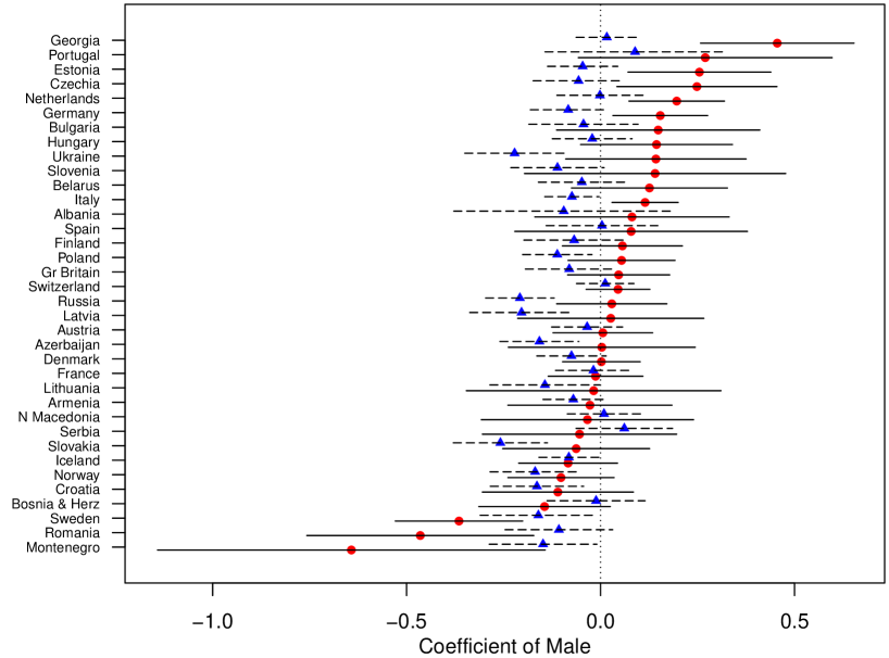
Figure 1: Estimates of the coefficient (with 95% confidence intervals) of dummy variable for men in models for intrinsic work values (circles and solid lines) and extrinsic work values (triangles and dashed lines). Two-step estimates obtained separately for each country in the 2017 European Values Survey, but with the same measurement model for each country estimated from pooled data in step 1.

Note: The coefficients are expressed on a scale where the residual variance of both factors for the Netherlands is 1. The models also include as covariates the respondent’s age, education, social class and employment status (working vs. not).

We allow all parameters of the structural model (regression coefficients and residual variances and covariance) to have different values in each country. Every parameter of the measurement model, in contrast, is constrained to have the same value in all countries, to specify full measurement equivalence across the countries. We note that because the step-1 estimates are here based on much more data than the step-2 estimates (with nearly 59,000 observations in the pooled data but 1000–2000 in each country), step 1 contributes essentially nothing to the standard errors of the estimated structural coefficients. So in this example we could safely treat the measurement parameters from step 1 as known and omit the term for them from the estimated standard errors.

Two-, one- and three-step estimates of gender differences in the work values in each country are shown in supplementary Tables B.3 and B.4. We focus here on the two-step estimates, which are also shown in Figure 1. For extrinsic values, most of the point estimates indicate higher average importance of them for women, but these differences are small and mostly not statistically significant (at the 5% level). For intrinsic values there are a few more countries with significant differences, but they include ones in both directions and have no very clear geographic regularities in the variation across countries. In other words, these results do not show strong evidence of consistent gender differences in work value orientations, suggesting at best small differences with much cross-national variation in them.

As mentioned at the start of this this section, this application example also allowed us to examine two topics in the relative performance of two-step estimation. From the analysis for the Netherlands above, we discussed the observed level of interpretative confounding in one-step estimates. The second, cross-national analysis provides an extreme illustration of the difference in computational convenience between two- and one-step estimation. The model has 836 estimable parameters. One-step estimates have to be calculated for all of them at once, from the pooled dataset of all the countries. On our computer this took 4.5 hours, using just one starting value. Two-step estimation, in contrast, splits the task in a way which considerably simplifies it. In its step 1, the measurement models are estimated from the pooled dataset, as two one-factor models for three binary items each and without any covariates. Step 2 can then be done separately for each country, because their structural parameters are distinct. Even with multiple starting values (Starts=30 10 in Mplus syntax) this took just 1-2 minutes for both step 1 and each country in step 2, for a total of a little over 0.5 hours for the whole model.

6 Conclusions and discussion

Two-step estimation is a general approach which is in principle applicable to any types of latent variable models where the focus of interest is on the structural model. In this paper we have described it for the broad family of latent trait (or item response theory) models, where continuous latent variables are measured by observed categorical indicators. In our simulations and examples, two-step estimation performed very well for them, as was also expected on theoretical grounds. This is also in line with previous findings on two-step estimation for other families of models, in particular latent class analysis of categorical variables and structural equation modelling of continuous variables. Together these studies provide increasingly strong evidence and reassurance that the two-step method is a useful and convenient approach to estimation of latent variable models in general, and an attractive alternative to the existing one-step and three-step methods.

We also considered whether the different potential advantages of two-step estimation were more or less prominent here than for other families of models. One of them is practical and computational convenience, compared to one-step estimation of all parts of the model at once. This advantage may be particularly important for latent trait models, because they are more often used with complex structural models than are latent class models, and are also inherently more computationally demanding than structural equation models. Another attractive characteristic of the two-step approach is that it avoids interpretational confounding, where the effective definition of the latent variables is affected by the specification of the structural model. This may be more consequential for latent class models, where the interpretation of a categorical latent class variable can change in a discontinuous way, than for latent trait models and structural equation models which have continuous latent variables. However, interpretational confounding is also an instance of the broader problem of biases that can be induced when the models are misspecified. Two-step estimation is also expected to provide some protection against them in any types of models.

To build on these promising results so far, different directions of further research on different elements of two-step estimation could be pursued. The accessibility of the approach would be much improved by integrated implementation of it (including calculation of correct standard errors of the estimates) in general-purpose software for latent variable models, including latent trait models. This would extend and complement the procedures that have already become available for latent class and structural equation modelling. For better understanding of the scope of two-step estimation, its implementation and performance could be studied for other categories of models, for example ones which combine different types of latent variables and measurement items, or for extensions such as multilevel models and ones with non-equivalent measurement models. These and other areas of further research remain to be explored.

These supplementary materials provide the following information:

Appendix A Results of the simulations (Section 4 of the paper)

• Path diagrams that represent the cases 1, 2, and 3 that are considered in the simulations of Section 4 of the paper are shown in Figure A.1.

• Full results of the simulations are given Tables A.1–A.10:

  • Case 1 (Observed covariate, latent response) in Tables A.1–A.2 (point estimates) and A.6–A.7 (standard errors and confidence intervals).

  • Case 2 (Latent covariate, observed response) in Tables A.3–A.4 (point estimates) and A.8–A.9 (standard errors and confidence intervals).

  • Case 3 (Latent covariate, latent response) in Tables A.5 (point estimates) and A.10 (standard errors and confidence intervals).

    • The tables for Case 3 (A.5 and A.10) are also shown in Section 4, as Tables 1 and 2 respectively.

Appendix B Results of the example (Section 5 of the paper)

Further results of the applied example discussed in Section 5 of the paper are given Tables B.1–B.4:

• The full sets of estimated coefficients for the structural models for Netherlands in Tables B.1–B.2.

  • Of these, the results for the coefficient of the dummy variable for Male are also shown in Section 5, as part of Table 3.

• The list of countries in the cross-national analysis, their sample sizes, and estimated coefficients of the dummy variable for Male in each of them in Tables B.3–B.4.

  • Of these, the two-step estimates of the coefficients and their 95% confidence intervals are also displayed in Figure 1 in Section 5 (with the further standardisation that there the coefficients are expressed on a scale where the residual variance of both intrinsic and exterinsic values for the Netherlands is 1).

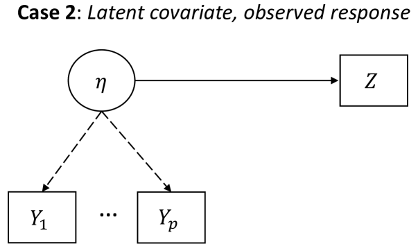
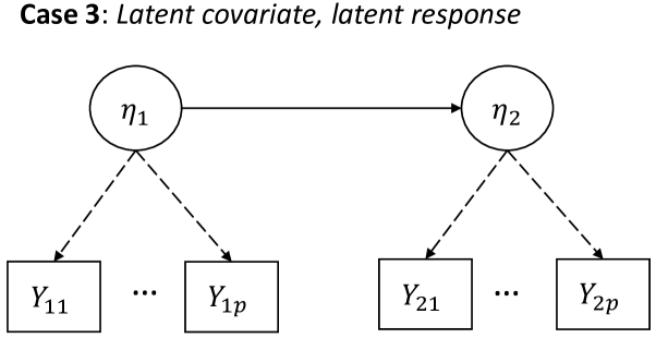
Figure A.1: Path diagrams representing the three cases that are considered in the simulation studies of Section 4 of the paper. Here the dashed arrows represent the measurement model that is estimated in step 1 of two-step estimation, and the solid arrow the structural model (regression model for $\eta$ given $X$, $Z$ given $\eta$, or $\eta_{2}$ given $\eta_{1}$) that is estimated in its step 2.

Table A.1: Simulation results for point estimates of structural regression coefficient $\beta_{1}$ of a normally distributed covariate $X$ for a latent response $\eta$ (simulation Case 1(a)) .

					Bias			RMSE			MAE
$p$	$\pi_{Y}$	$R^{2}_{Y}$	$R^{2}_{\eta}$	$\beta_{1}$	2-step	1-step	3-step	2-step	1-step	3-step	2-step	1-step	3-step
$n=200$
4	0.5	0.4	0.0	0.000	-0.003	-0.004	-0.002	0.146	0.151	0.090	0.084	0.086	0.052
4	0.8	0.4	0.0	0.000	0.007	0.006	0.003	0.196	0.208	0.094	0.100	0.102	0.045
4	0.5	0.6	0.0	0.000	0.008	0.008	0.006	0.207	0.208	0.145	0.125	0.126	0.086
4	0.8	0.6	0.0	0.000	0.002	0.002	0.002	0.251	0.253	0.151	0.144	0.145	0.085
8	0.5	0.4	0.0	0.000	-0.005	-0.005	-0.004	0.132	0.132	0.098	0.085	0.085	0.063
8	0.8	0.4	0.0	0.000	0.003	0.003	0.002	0.150	0.152	0.088	0.096	0.097	0.056
8	0.5	0.6	0.0	0.000	0.004	0.004	0.003	0.187	0.185	0.150	0.118	0.118	0.095
8	0.8	0.6	0.0	0.000	-0.013	-0.013	-0.009	0.203	0.204	0.141	0.133	0.135	0.093
4	0.5	0.4	0.2	0.662	0.030	0.039	-0.239	0.251	0.229	0.292	0.137	0.132	0.267
4	0.8	0.4	0.2	0.662	0.065	0.054	-0.326	0.527	0.367	0.423	0.179	0.166	0.382
4	0.5	0.6	0.2	0.993	0.045	0.048	-0.270	0.320	0.300	0.355	0.182	0.176	0.319
4	0.8	0.6	0.2	0.993	0.085	0.071	-0.359	0.520	0.394	0.475	0.221	0.210	0.418
8	0.5	0.4	0.2	0.662	0.023	0.026	-0.153	0.183	0.180	0.208	0.119	0.115	0.175
8	0.8	0.4	0.2	0.662	0.031	0.040	-0.254	0.255	0.266	0.298	0.151	0.142	0.277
8	0.5	0.6	0.2	0.993	0.042	0.042	-0.163	0.256	0.253	0.262	0.161	0.162	0.205
8	0.8	0.6	0.2	0.993	0.052	0.056	-0.264	0.315	0.312	0.345	0.188	0.190	0.302
4	0.5	0.4	0.4	0.937	0.031	0.034	-0.348	0.305	0.251	0.401	0.185	0.148	0.382
4	0.8	0.4	0.4	0.937	0.143	0.074	-0.443	0.924	0.365	0.632	0.254	0.213	0.533
4	0.5	0.6	0.4	1.405	0.083	0.071	-0.367	0.404	0.364	0.466	0.233	0.207	0.412
4	0.8	0.6	0.4	1.405	0.093	0.075	-0.527	0.642	0.449	0.663	0.269	0.252	0.611
8	0.5	0.4	0.4	0.937	0.035	0.042	-0.216	0.234	0.233	0.280	0.136	0.131	0.245
8	0.8	0.4	0.4	0.937	0.040	0.051	-0.362	0.309	0.297	0.408	0.183	0.167	0.389
8	0.5	0.6	0.4	1.405	0.051	0.051	-0.239	0.317	0.316	0.351	0.198	0.197	0.286
8	0.8	0.6	0.4	1.405	0.051	0.054	-0.391	0.365	0.356	0.470	0.214	0.207	0.434
$n=1000$
4	0.5	0.4	0.0	0.000	0.000	0.000	0.000	0.062	0.062	0.037	0.041	0.041	0.025
4	0.8	0.4	0.0	0.000	0.005	0.005	0.002	0.073	0.074	0.033	0.046	0.046	0.020
4	0.5	0.6	0.0	0.000	0.002	0.002	0.001	0.086	0.086	0.060	0.058	0.058	0.040
4	0.8	0.6	0.0	0.000	0.007	0.007	0.004	0.095	0.095	0.055	0.065	0.065	0.038
8	0.5	0.4	0.0	0.000	0.000	0.000	0.000	0.055	0.055	0.041	0.036	0.036	0.026
8	0.8	0.4	0.0	0.000	-0.003	-0.003	-0.002	0.065	0.065	0.038	0.044	0.044	0.026
8	0.5	0.6	0.0	0.000	0.002	0.002	0.002	0.080	0.079	0.064	0.052	0.051	0.041
8	0.8	0.6	0.0	0.000	-0.001	-0.001	-0.000	0.085	0.085	0.059	0.057	0.057	0.040
4	0.5	0.4	0.2	0.662	-0.004	-0.001	-0.268	0.098	0.092	0.276	0.063	0.059	0.273
4	0.8	0.4	0.2	0.662	0.009	0.014	-0.365	0.117	0.108	0.369	0.078	0.072	0.369
4	0.5	0.6	0.2	0.993	0.015	0.016	-0.292	0.127	0.123	0.307	0.084	0.079	0.300
4	0.8	0.6	0.2	0.993	0.006	0.007	-0.409	0.143	0.137	0.419	0.095	0.093	0.413
8	0.5	0.4	0.2	0.662	0.003	0.004	-0.171	0.077	0.076	0.181	0.054	0.052	0.174
8	0.8	0.4	0.2	0.662	0.003	0.003	-0.273	0.095	0.093	0.280	0.066	0.063	0.277
8	0.5	0.6	0.2	0.993	-0.001	-0.002	-0.199	0.108	0.108	0.218	0.072	0.073	0.201
8	0.8	0.6	0.2	0.993	0.001	0.001	-0.299	0.116	0.115	0.310	0.078	0.077	0.304
4	0.5	0.4	0.4	0.937	0.008	0.011	-0.371	0.123	0.107	0.380	0.080	0.070	0.378
4	0.8	0.4	0.4	0.937	0.012	0.014	-0.517	0.158	0.133	0.523	0.096	0.086	0.524
4	0.5	0.6	0.4	1.405	0.013	0.014	-0.420	0.157	0.151	0.436	0.099	0.097	0.426
4	0.8	0.6	0.4	1.405	0.011	0.011	-0.579	0.184	0.170	0.591	0.120	0.116	0.586
8	0.5	0.4	0.4	0.937	0.006	0.007	-0.241	0.097	0.093	0.252	0.062	0.060	0.243
8	0.8	0.4	0.4	0.937	0.009	0.010	-0.385	0.121	0.114	0.392	0.082	0.075	0.388
8	0.5	0.6	0.4	1.405	0.007	0.007	-0.275	0.125	0.123	0.293	0.079	0.079	0.278
8	0.8	0.6	0.4	1.405	0.020	0.018	-0.410	0.153	0.150	0.425	0.100	0.096	0.412
Note: $p$ denotes number of measurement items $Y_{j}$, $\pi_{Y}$ marginal proportion of $Y_{j}=1$,
$R_{Y}^{2}$ and $R^{2}_{\eta}$ the $R^{2}$ statistics in models for $Y_{j}$ and $\eta$, and $\beta_{1}$ true value of $\beta_{1}$.

Table A.2: Simulation results for point estimates of structural regression coefficient $\beta_{1}$ of a binary covariate $X$ for a latent response $\eta$ (Case 1(b)).

					Bias			RMSE			MAE
$p$	$\pi_{Y}$	$R^{2}_{Y}$	$R^{2}_{\eta}$	$\beta_{1}$	2-step	1-step	3-step	2-step	1-step	3-step	2-step	1-step	3-step
$n=200$
4	0.5	0.4	0.0	0.000	0.001	0.001	0.000	0.144	0.147	0.090	0.090	0.092	0.055
4	0.8	0.4	0.0	0.000	0.007	0.008	0.003	0.191	0.213	0.091	0.099	0.106	0.046
4	0.5	0.6	0.0	0.000	-0.001	-0.002	-0.001	0.209	0.210	0.147	0.129	0.129	0.091
4	0.8	0.6	0.0	0.000	0.002	0.001	0.001	0.259	0.254	0.160	0.138	0.141	0.081
8	0.5	0.4	0.0	0.000	-0.002	-0.002	-0.002	0.125	0.126	0.093	0.086	0.086	0.063
8	0.8	0.4	0.0	0.000	0.004	0.005	0.003	0.160	0.162	0.095	0.091	0.092	0.053
8	0.5	0.6	0.0	0.000	-0.005	-0.005	-0.004	0.185	0.184	0.149	0.126	0.126	0.100
8	0.8	0.6	0.0	0.000	0.005	0.005	0.003	0.204	0.206	0.143	0.135	0.135	0.094
4	0.5	0.4	0.2	0.662	0.016	0.026	-0.231	0.236	0.221	0.285	0.138	0.135	0.261
4	0.8	0.4	0.2	0.662	0.077	0.050	-0.318	0.567	0.316	0.439	0.194	0.171	0.383
4	0.5	0.6	0.2	0.993	0.035	0.037	-0.236	0.299	0.297	0.332	0.191	0.182	0.290
4	0.8	0.6	0.2	0.993	0.082	0.083	-0.345	0.465	0.428	0.444	0.218	0.211	0.393
8	0.5	0.4	0.2	0.662	0.021	0.023	-0.137	0.192	0.189	0.208	0.126	0.124	0.169
8	0.8	0.4	0.2	0.662	0.018	0.026	-0.257	0.239	0.232	0.298	0.147	0.140	0.277
8	0.5	0.6	0.2	0.993	0.044	0.044	-0.123	0.256	0.255	0.254	0.157	0.158	0.191
8	0.8	0.6	0.2	0.993	0.046	0.048	-0.248	0.309	0.303	0.336	0.180	0.178	0.290
4	0.5	0.4	0.4	0.937	0.042	0.039	-0.280	0.308	0.236	0.361	0.171	0.156	0.323
4	0.8	0.4	0.4	0.937	0.062	0.065	-0.479	0.587	0.388	0.563	0.234	0.182	0.525
4	0.5	0.6	0.4	1.405	0.050	0.045	-0.254	0.398	0.351	0.425	0.223	0.198	0.337
4	0.8	0.6	0.4	1.405	0.079	0.072	-0.495	0.508	0.505	0.594	0.253	0.241	0.558
8	0.5	0.4	0.4	0.937	0.015	0.018	-0.175	0.217	0.208	0.255	0.137	0.131	0.204
8	0.8	0.4	0.4	0.937	0.025	0.037	-0.361	0.290	0.279	0.406	0.181	0.164	0.381
8	0.5	0.6	0.4	1.405	0.047	0.044	-0.114	0.321	0.308	0.320	0.185	0.175	0.229
8	0.8	0.6	0.4	1.405	0.070	0.071	-0.318	0.359	0.352	0.419	0.216	0.213	0.365
$n=1000$
4	0.5	0.4	0.0	0.000	-0.000	-0.000	0.000	0.061	0.062	0.037	0.040	0.040	0.024
4	0.8	0.4	0.0	0.000	0.000	0.000	0.000	0.073	0.074	0.032	0.046	0.046	0.020
4	0.5	0.6	0.0	0.000	-0.002	-0.002	-0.001	0.082	0.083	0.058	0.055	0.056	0.039
4	0.8	0.6	0.0	0.000	0.003	0.003	0.002	0.094	0.094	0.055	0.060	0.060	0.035
8	0.5	0.4	0.0	0.000	0.001	0.001	0.001	0.056	0.056	0.042	0.037	0.037	0.027
8	0.8	0.4	0.0	0.000	0.002	0.002	0.001	0.064	0.064	0.037	0.044	0.043	0.025
8	0.5	0.6	0.0	0.000	-0.002	-0.002	-0.001	0.081	0.081	0.065	0.056	0.055	0.045
8	0.8	0.6	0.0	0.000	0.005	0.005	0.004	0.087	0.087	0.061	0.055	0.055	0.038
4	0.5	0.4	0.2	0.662	0.004	0.005	-0.249	0.093	0.086	0.257	0.058	0.055	0.253
4	0.8	0.4	0.2	0.662	0.001	0.009	-0.366	0.128	0.114	0.371	0.081	0.072	0.370
4	0.5	0.6	0.2	0.993	0.008	0.011	-0.261	0.118	0.118	0.278	0.077	0.078	0.263
4	0.8	0.6	0.2	0.993	-0.002	-0.001	-0.401	0.145	0.140	0.412	0.093	0.093	0.408
8	0.5	0.4	0.2	0.662	0.007	0.007	-0.152	0.079	0.078	0.165	0.053	0.052	0.156
8	0.8	0.4	0.2	0.662	0.008	0.009	-0.266	0.096	0.094	0.273	0.061	0.059	0.268
8	0.5	0.6	0.2	0.993	0.003	0.002	-0.161	0.109	0.109	0.187	0.069	0.070	0.164
8	0.8	0.6	0.2	0.993	0.008	0.009	-0.276	0.118	0.118	0.290	0.082	0.079	0.279
4	0.5	0.4	0.4	0.937	0.001	0.005	-0.322	0.119	0.103	0.334	0.077	0.069	0.330
4	0.8	0.4	0.4	0.937	0.005	0.011	-0.520	0.165	0.131	0.526	0.105	0.085	0.525
4	0.5	0.6	0.4	1.405	0.007	0.012	-0.296	0.154	0.141	0.325	0.105	0.097	0.308
4	0.8	0.6	0.4	1.405	0.023	0.020	-0.531	0.182	0.166	0.545	0.122	0.102	0.541
8	0.5	0.4	0.4	0.937	0.001	0.003	-0.191	0.095	0.089	0.208	0.062	0.057	0.194
8	0.8	0.4	0.4	0.937	0.006	0.010	-0.376	0.114	0.111	0.383	0.072	0.072	0.377
8	0.5	0.6	0.4	1.405	0.014	0.014	-0.148	0.129	0.124	0.191	0.085	0.083	0.161
8	0.8	0.6	0.4	1.405	0.007	0.005	-0.364	0.148	0.143	0.382	0.097	0.094	0.372
Note: $p$ denotes number of measurement items $Y_{j}$, $\pi_{Y}$ marginal proportion of $Y_{j}=1$,
$R_{Y}^{2}$ and $R^{2}_{\eta}$ the $R^{2}$ statistics in models for $Y_{j}$ and $\eta$, and $\beta_{1}$ true value of $\beta_{1}$.

Table A.3: Simulation results for point estimates of structural regression coefficient $\beta_{1}$ of a latent covariate $\eta$ for a conditionally normally distributed response $Z$ (Case 2(a)).

					Bias			RMSE			MAE
$p$	$\pi_{Y}$	$R^{2}_{Y}$	$R^{2}_{Z}$	$\beta_{1}$	2-step	1-step	3-step	2-step	1-step	3-step	2-step	1-step	3-step
$n=200$
4	0.5	0.4	0.0	0.000	-0.003	-0.003	-0.003	0.067	0.070	0.067	0.041	0.042	0.040
4	0.8	0.4	0.0	0.000	-0.003	-0.003	-0.003	0.089	0.104	0.088	0.050	0.057	0.050
4	0.5	0.6	0.0	0.000	-0.000	-0.000	-0.000	0.039	0.040	0.039	0.024	0.025	0.024
4	0.8	0.6	0.0	0.000	-0.000	-0.000	-0.000	0.044	0.046	0.044	0.027	0.029	0.027
8	0.5	0.4	0.0	0.000	0.001	0.001	0.001	0.059	0.060	0.059	0.038	0.038	0.038
8	0.8	0.4	0.0	0.000	-0.002	-0.002	-0.002	0.068	0.071	0.068	0.042	0.043	0.042
8	0.5	0.6	0.0	0.000	0.002	0.002	0.002	0.038	0.038	0.037	0.025	0.025	0.025
8	0.8	0.6	0.0	0.000	0.001	0.001	0.001	0.040	0.040	0.040	0.025	0.025	0.025
4	0.5	0.4	0.2	0.302	0.003	0.012	0.003	0.111	0.113	0.111	0.072	0.071	0.071
4	0.8	0.4	0.2	0.302	0.008	0.027	0.008	0.159	0.159	0.156	0.088	0.087	0.090
4	0.5	0.6	0.2	0.201	-0.000	0.003	0.000	0.060	0.061	0.061	0.041	0.040	0.041
4	0.8	0.6	0.2	0.201	-0.005	-0.000	-0.004	0.065	0.063	0.066	0.044	0.042	0.044
8	0.5	0.4	0.2	0.302	-0.004	0.001	-0.004	0.083	0.085	0.083	0.056	0.057	0.056
8	0.8	0.4	0.2	0.302	0.005	0.018	0.006	0.114	0.119	0.114	0.070	0.068	0.069
8	0.5	0.6	0.2	0.201	0.000	0.001	0.000	0.051	0.051	0.051	0.035	0.034	0.035
8	0.8	0.6	0.2	0.201	-0.002	0.001	-0.002	0.055	0.056	0.056	0.037	0.038	0.037
4	0.5	0.4	0.4	0.427	0.002	0.012	0.003	0.134	0.129	0.134	0.083	0.082	0.084
4	0.8	0.4	0.4	0.427	-0.001	0.028	0.006	0.181	0.191	0.188	0.101	0.091	0.104
4	0.5	0.6	0.4	0.285	0.001	0.002	0.002	0.073	0.070	0.074	0.049	0.045	0.050
4	0.8	0.6	0.4	0.285	-0.005	0.003	-0.003	0.086	0.082	0.087	0.057	0.056	0.058
8	0.5	0.4	0.4	0.427	0.005	0.013	0.005	0.107	0.107	0.107	0.067	0.070	0.070
8	0.8	0.4	0.4	0.427	0.008	0.024	0.010	0.137	0.146	0.139	0.083	0.083	0.084
8	0.5	0.6	0.4	0.285	0.002	0.003	0.002	0.061	0.061	0.061	0.039	0.040	0.039
8	0.8	0.6	0.4	0.285	-0.003	0.002	-0.003	0.067	0.068	0.067	0.044	0.045	0.046
$n=1000$
4	0.5	0.4	0.0	0.000	-0.000	-0.000	-0.000	0.028	0.029	0.028	0.019	0.019	0.019
4	0.8	0.4	0.0	0.000	-0.001	-0.001	-0.001	0.034	0.034	0.034	0.022	0.022	0.022
4	0.5	0.6	0.0	0.000	0.000	0.000	0.000	0.017	0.018	0.017	0.012	0.012	0.012
4	0.8	0.6	0.0	0.000	-0.000	-0.000	-0.000	0.020	0.020	0.020	0.012	0.012	0.012
8	0.5	0.4	0.0	0.000	-0.001	-0.001	-0.001	0.026	0.026	0.025	0.016	0.016	0.016
8	0.8	0.4	0.0	0.000	0.002	0.002	0.002	0.030	0.030	0.030	0.019	0.020	0.020
8	0.5	0.6	0.0	0.000	0.001	0.001	0.001	0.016	0.016	0.016	0.011	0.011	0.011
8	0.8	0.6	0.0	0.000	0.000	0.000	0.000	0.017	0.017	0.017	0.011	0.011	0.011
4	0.5	0.4	0.2	0.302	0.003	0.003	0.002	0.046	0.044	0.046	0.030	0.029	0.030
4	0.8	0.4	0.2	0.302	0.006	0.008	0.007	0.060	0.057	0.061	0.041	0.039	0.040
4	0.5	0.6	0.2	0.201	-0.001	0.000	-0.001	0.026	0.025	0.026	0.017	0.017	0.017
4	0.8	0.6	0.2	0.201	-0.002	-0.001	-0.002	0.031	0.030	0.031	0.022	0.021	0.021
8	0.5	0.4	0.2	0.302	-0.000	0.001	-0.001	0.035	0.035	0.035	0.023	0.023	0.023
8	0.8	0.4	0.2	0.302	-0.000	0.003	-0.000	0.045	0.046	0.046	0.031	0.031	0.031
8	0.5	0.6	0.2	0.201	-0.002	-0.001	-0.002	0.022	0.022	0.022	0.015	0.015	0.015
8	0.8	0.6	0.2	0.201	0.000	0.001	-0.000	0.025	0.025	0.025	0.016	0.017	0.017
4	0.5	0.4	0.4	0.427	0.002	0.003	0.002	0.058	0.052	0.058	0.039	0.034	0.039
4	0.8	0.4	0.4	0.427	-0.001	0.002	-0.002	0.074	0.065	0.074	0.049	0.043	0.050
4	0.5	0.6	0.4	0.285	0.001	0.002	0.001	0.031	0.030	0.031	0.021	0.020	0.021
4	0.8	0.6	0.4	0.285	0.000	0.002	0.000	0.037	0.034	0.037	0.025	0.022	0.026
8	0.5	0.4	0.4	0.427	-0.001	0.001	-0.001	0.044	0.043	0.044	0.029	0.028	0.029
8	0.8	0.4	0.4	0.427	-0.001	0.003	-0.001	0.053	0.052	0.053	0.035	0.034	0.035
8	0.5	0.6	0.4	0.285	-0.000	-0.000	-0.000	0.026	0.026	0.026	0.017	0.017	0.018
8	0.8	0.6	0.4	0.285	0.000	0.001	0.000	0.028	0.029	0.029	0.019	0.019	0.020
Note: $p$ denotes number of measurement items $Y_{j}$, $\pi_{Y}$ marginal proportion of $Y_{j}=1$,
$R_{Y}^{2}$ and $R^{2}_{Z}$ the $R^{2}$ statistics in models for $Y_{j}$ and $Z$, and $\beta_{1}$ true value of $\beta_{1}$.

Table A.4: Simulation results for point estimates of structural regression coefficient $\beta_{1}$ of a latent covariate $\eta$ for a conditionally skew-normally distributed response $Z$ (Case 2(b)).

					Bias			RMSE			MAE
$p$	$\pi_{Y}$	$R^{2}_{Y}$	$R^{2}_{Z}$	$\beta_{1}$	2-step	1-step	3-step	2-step	1-step	3-step	2-step	1-step	3-step
$n=200$
4	0.5	0.4	0.0	0.000	0.003	0.003	0.003	0.068	0.070	0.067	0.040	0.042	0.040
4	0.8	0.4	0.0	0.000	0.005	0.008	0.003	0.085	0.113	0.084	0.043	0.048	0.043
4	0.5	0.6	0.0	0.000	0.000	0.000	0.000	0.039	0.040	0.039	0.025	0.026	0.025
4	0.8	0.6	0.0	0.000	0.001	0.001	-0.000	0.044	0.046	0.044	0.026	0.027	0.026
8	0.5	0.4	0.0	0.000	0.002	0.002	0.002	0.056	0.057	0.056	0.037	0.038	0.037
8	0.8	0.4	0.0	0.000	0.001	0.001	-0.000	0.064	0.067	0.064	0.041	0.043	0.041
8	0.5	0.6	0.0	0.000	-0.000	-0.000	-0.000	0.036	0.036	0.036	0.024	0.025	0.024
8	0.8	0.6	0.0	0.000	0.004	0.004	0.003	0.040	0.040	0.040	0.026	0.026	0.026
4	0.5	0.4	0.2	0.302	0.007	0.016	0.007	0.114	0.113	0.113	0.071	0.067	0.070
4	0.8	0.4	0.2	0.302	0.022	0.043	0.008	0.173	0.193	0.160	0.093	0.090	0.089
4	0.5	0.6	0.2	0.201	-0.002	0.001	-0.002	0.059	0.057	0.059	0.038	0.036	0.038
4	0.8	0.6	0.2	0.201	0.008	0.014	0.001	0.076	0.076	0.071	0.048	0.047	0.048
8	0.5	0.4	0.2	0.302	0.004	0.009	0.004	0.086	0.088	0.085	0.057	0.058	0.057
8	0.8	0.4	0.2	0.302	0.019	0.035	0.010	0.119	0.128	0.111	0.069	0.069	0.066
8	0.5	0.6	0.2	0.201	-0.001	0.001	-0.001	0.050	0.050	0.050	0.034	0.034	0.034
8	0.8	0.6	0.2	0.201	0.005	0.010	0.000	0.059	0.061	0.055	0.037	0.037	0.035
4	0.5	0.4	0.4	0.427	-0.000	0.014	-0.000	0.142	0.133	0.142	0.088	0.082	0.087
4	0.8	0.4	0.4	0.427	0.020	0.052	0.009	0.193	0.206	0.194	0.107	0.097	0.109
4	0.5	0.6	0.4	0.285	-0.003	0.002	-0.003	0.072	0.068	0.072	0.050	0.046	0.049
4	0.8	0.6	0.4	0.285	0.006	0.015	-0.001	0.089	0.088	0.087	0.056	0.053	0.055
8	0.5	0.4	0.4	0.427	0.003	0.012	0.002	0.112	0.112	0.111	0.071	0.074	0.071
8	0.8	0.4	0.4	0.427	0.020	0.034	0.010	0.145	0.150	0.140	0.087	0.083	0.085
8	0.5	0.6	0.4	0.285	0.001	0.003	0.001	0.062	0.063	0.062	0.040	0.040	0.040
8	0.8	0.6	0.4	0.285	0.003	0.009	-0.002	0.069	0.070	0.067	0.046	0.046	0.045
$n=1000$
4	0.5	0.4	0.0	0.000	0.001	0.001	0.001	0.029	0.029	0.029	0.019	0.019	0.019
4	0.8	0.4	0.0	0.000	0.000	0.000	-0.000	0.033	0.033	0.032	0.021	0.021	0.021
4	0.5	0.6	0.0	0.000	0.000	0.000	0.000	0.018	0.018	0.018	0.012	0.012	0.012
4	0.8	0.6	0.0	0.000	0.001	0.001	0.001	0.018	0.018	0.018	0.013	0.013	0.013
8	0.5	0.4	0.0	0.000	-0.000	-0.000	-0.000	0.024	0.025	0.024	0.016	0.016	0.016
8	0.8	0.4	0.0	0.000	0.001	0.001	0.001	0.028	0.029	0.028	0.018	0.019	0.019
8	0.5	0.6	0.0	0.000	0.000	0.000	0.000	0.017	0.017	0.017	0.011	0.011	0.011
8	0.8	0.6	0.0	0.000	0.001	0.001	0.001	0.017	0.017	0.017	0.011	0.011	0.011
4	0.5	0.4	0.2	0.302	0.001	0.002	0.000	0.045	0.043	0.045	0.030	0.029	0.030
4	0.8	0.4	0.2	0.302	0.017	0.021	0.003	0.065	0.064	0.058	0.040	0.037	0.038
4	0.5	0.6	0.2	0.201	0.000	0.002	0.000	0.026	0.025	0.026	0.017	0.016	0.017
4	0.8	0.6	0.2	0.201	0.007	0.007	0.000	0.033	0.032	0.030	0.021	0.021	0.020
8	0.5	0.4	0.2	0.302	0.001	0.003	0.001	0.035	0.036	0.035	0.023	0.023	0.023
8	0.8	0.4	0.2	0.302	0.008	0.013	-0.000	0.048	0.050	0.045	0.030	0.032	0.029
8	0.5	0.6	0.2	0.201	-0.001	-0.001	-0.001	0.022	0.022	0.022	0.015	0.015	0.014
8	0.8	0.6	0.2	0.201	0.004	0.005	-0.000	0.025	0.025	0.024	0.017	0.017	0.016
4	0.5	0.4	0.4	0.427	0.005	0.007	0.004	0.059	0.053	0.058	0.039	0.033	0.038
4	0.8	0.4	0.4	0.427	0.025	0.029	0.004	0.084	0.076	0.076	0.051	0.047	0.049
4	0.5	0.6	0.4	0.285	0.001	0.001	0.000	0.032	0.031	0.032	0.022	0.021	0.022
4	0.8	0.6	0.4	0.285	0.011	0.014	0.002	0.040	0.039	0.037	0.025	0.026	0.023
8	0.5	0.4	0.4	0.427	-0.000	0.002	-0.000	0.044	0.042	0.044	0.029	0.028	0.029
8	0.8	0.4	0.4	0.427	0.012	0.015	0.001	0.059	0.057	0.055	0.038	0.035	0.035
8	0.5	0.6	0.4	0.285	-0.001	-0.001	-0.001	0.025	0.025	0.025	0.017	0.017	0.017
8	0.8	0.6	0.4	0.285	0.006	0.007	-0.000	0.030	0.031	0.029	0.019	0.019	0.019
Note: $p$ denotes number of measurement items $Y_{j}$, $\pi_{Y}$ marginal proportion of $Y_{j}=1$,
$R_{Y}^{2}$ and $R^{2}_{Z}$ the $R^{2}$ statistics in models for $Y_{j}$ and $Z$, and $\beta_{1}$ true value of $\beta_{1}$.

Table A.5: Simulation results for point estimates of structural regression coefficient $\beta_{1}$ of a latent covariate $\eta_{1}$ for a conditionally normally distributed latent response $\eta_{2}$ (Case 3).

					Bias			RMSE			MAE
$p$	$\pi_{Y}$	$R^{2}_{Y}$	$R^{2}_{\eta}$	$\beta_{1}$	2-step	1-step	3-step	2-step	1-step	3-step	2-step	1-step	3-step
$n=200$
4	0.5	0.4	0.0	0.000	-0.004	-0.003	-0.002	0.133	0.141	0.081	0.077	0.080	0.046
4	0.8	0.4	0.0	0.000	-0.007	-0.004	-0.000	0.240	0.276	0.110	0.101	0.113	0.044
4	0.5	0.6	0.0	0.000	0.007	0.007	0.005	0.115	0.117	0.080	0.069	0.070	0.048
4	0.8	0.6	0.0	0.000	0.002	0.002	0.003	0.153	0.154	0.091	0.081	0.084	0.048
8	0.5	0.4	0.0	0.000	-0.001	-0.001	-0.001	0.104	0.104	0.078	0.063	0.062	0.047
8	0.8	0.4	0.0	0.000	0.008	0.009	0.006	0.147	0.151	0.087	0.081	0.083	0.047
8	0.5	0.6	0.0	0.000	-0.003	-0.003	-0.002	0.097	0.095	0.077	0.062	0.059	0.050
8	0.8	0.6	0.0	0.000	-0.002	-0.002	-0.000	0.114	0.116	0.080	0.072	0.073	0.050
4	0.5	0.4	0.2	0.447	0.016	0.035	-0.162	0.236	0.237	0.221	0.132	0.132	0.202
4	0.8	0.4	0.2	0.447	0.031	0.070	-0.208	0.404	0.385	0.300	0.183	0.177	0.267
4	0.5	0.6	0.2	0.447	0.019	0.025	-0.116	0.182	0.189	0.176	0.117	0.116	0.148
4	0.8	0.6	0.2	0.447	0.030	0.039	-0.144	0.257	0.244	0.225	0.135	0.134	0.183
8	0.5	0.4	0.2	0.447	0.013	0.010	-0.104	0.177	0.188	0.170	0.109	0.110	0.137
8	0.8	0.4	0.2	0.447	0.023	0.040	-0.152	0.249	0.250	0.222	0.144	0.136	0.197
8	0.5	0.6	0.2	0.447	0.005	-0.008	-0.081	0.143	0.159	0.143	0.092	0.093	0.116
8	0.8	0.6	0.2	0.447	0.024	0.028	-0.100	0.183	0.181	0.170	0.114	0.111	0.137
4	0.5	0.4	0.4	0.632	0.028	0.047	-0.223	0.309	0.285	0.301	0.176	0.162	0.268
4	0.8	0.4	0.4	0.632	0.042	0.081	-0.284	0.608	0.457	0.436	0.228	0.199	0.363
4	0.5	0.6	0.4	0.632	0.048	0.052	-0.143	0.275	0.254	0.247	0.140	0.147	0.199
4	0.8	0.6	0.4	0.632	0.038	0.048	-0.195	0.326	0.283	0.295	0.174	0.161	0.255
8	0.5	0.4	0.4	0.632	0.020	0.022	-0.142	0.213	0.222	0.216	0.131	0.134	0.176
8	0.8	0.4	0.4	0.632	0.033	0.054	-0.204	0.344	0.346	0.309	0.177	0.166	0.258
8	0.5	0.6	0.4	0.632	0.033	0.006	-0.087	0.196	0.227	0.182	0.127	0.124	0.138
8	0.8	0.6	0.4	0.632	0.024	0.030	-0.138	0.223	0.218	0.220	0.137	0.135	0.180
$n=1000$
4	0.5	0.4	0.0	0.000	0.000	0.000	0.000	0.053	0.054	0.032	0.036	0.036	0.021
4	0.8	0.4	0.0	0.000	-0.001	-0.001	-0.000	0.072	0.073	0.032	0.049	0.049	0.021
4	0.5	0.6	0.0	0.000	-0.001	-0.001	-0.001	0.045	0.045	0.031	0.030	0.030	0.021
4	0.8	0.6	0.0	0.000	0.001	0.001	0.001	0.054	0.055	0.032	0.036	0.036	0.021
8	0.5	0.4	0.0	0.000	0.000	0.000	0.000	0.045	0.045	0.033	0.031	0.031	0.023
8	0.8	0.4	0.0	0.000	0.001	0.001	0.001	0.059	0.059	0.034	0.038	0.038	0.022
8	0.5	0.6	0.0	0.000	-0.001	-0.001	-0.000	0.040	0.040	0.032	0.026	0.026	0.021
8	0.8	0.6	0.0	0.000	0.000	0.000	0.000	0.045	0.045	0.032	0.030	0.030	0.021
4	0.5	0.4	0.2	0.447	0.006	0.012	-0.174	0.092	0.090	0.183	0.061	0.059	0.178
4	0.8	0.4	0.2	0.447	0.011	0.021	-0.227	0.124	0.124	0.236	0.078	0.077	0.234
4	0.5	0.6	0.2	0.447	0.001	0.003	-0.131	0.075	0.074	0.142	0.053	0.052	0.135
4	0.8	0.6	0.2	0.447	0.011	0.013	-0.160	0.091	0.090	0.171	0.057	0.059	0.168
8	0.5	0.4	0.2	0.447	0.004	0.005	-0.112	0.073	0.073	0.125	0.047	0.047	0.116
8	0.8	0.4	0.2	0.447	0.010	0.015	-0.163	0.094	0.093	0.174	0.062	0.061	0.166
8	0.5	0.6	0.2	0.447	0.002	0.003	-0.084	0.062	0.062	0.098	0.039	0.039	0.087
8	0.8	0.6	0.2	0.447	0.008	0.009	-0.113	0.074	0.074	0.126	0.048	0.048	0.118
4	0.5	0.4	0.4	0.632	0.009	0.014	-0.244	0.118	0.112	0.255	0.076	0.076	0.250
4	0.8	0.4	0.4	0.632	0.003	0.014	-0.319	0.156	0.150	0.329	0.103	0.099	0.329
4	0.5	0.6	0.4	0.632	0.006	0.007	-0.177	0.093	0.090	0.190	0.061	0.058	0.182
4	0.8	0.6	0.4	0.632	0.009	0.010	-0.218	0.117	0.109	0.232	0.074	0.071	0.223
8	0.5	0.4	0.4	0.632	0.003	0.005	-0.158	0.088	0.086	0.172	0.059	0.057	0.164
8	0.8	0.4	0.4	0.632	-0.001	0.007	-0.231	0.114	0.111	0.244	0.078	0.072	0.237
8	0.5	0.6	0.4	0.632	0.007	0.008	-0.110	0.080	0.079	0.128	0.054	0.053	0.112
8	0.8	0.6	0.4	0.632	0.006	0.008	-0.152	0.088	0.086	0.167	0.060	0.058	0.156
Note: $p$ denotes number of measurement items $Y_{j}$, $\pi_{Y}$ marginal proportion of $Y_{j}=1$,
$R_{Y}^{2}$ and $R^{2}_{\eta}$ the $R^{2}$ statistics in models for $Y_{j}$ and $\eta_{2}$, and $\beta_{1}$ true value of $\beta_{1}$.

Table A.6: Simulation results for standard error estimates of structural regression coefficient $\beta_{1}$ of a normally distributed covariate $X$ for a latent response $\eta$ (Case 1(a)).

					Simulation standard deviation							2-step
					vs. mean of est. std. error				Coverage of			without
					2-step		1-step		95% conf. interval			step-1 var.†
$p$	$p_{Y}$	$R^{2}_{Y}$	$R^{2}_{\eta}$	$\beta_{1}$	s.d.	m(se)	s.d.	m(se)	2-st.	1-st.	3-st.	%var.	cover.
$n=200$
4	0.5	0.4	0.0	0.000	0.146	0.149	0.151	0.149	98.4	98.0	95.3	92.6	95.3
4	0.8	0.4	0.0	0.000	0.196	0.204	0.208	0.201	99.2	98.1	94.8	86.5	95.0
4	0.5	0.6	0.0	0.000	0.207	0.205	0.208	0.204	96.1	95.8	93.2	95.2	93.4
4	0.8	0.6	0.0	0.000	0.251	0.240	0.253	0.243	97.4	96.8	94.0	92.8	94.2
8	0.5	0.4	0.0	0.000	0.132	0.129	0.132	0.129	96.8	96.8	95.3	95.6	95.3
8	0.8	0.4	0.0	0.000	0.150	0.150	0.152	0.150	98.2	98.0	95.1	92.6	95.0
8	0.5	0.6	0.0	0.000	0.187	0.186	0.185	0.185	95.4	95.6	94.2	96.8	94.3
8	0.8	0.6	0.0	0.000	0.203	0.202	0.203	0.202	96.5	96.2	94.7	95.9	94.7
4	0.5	0.4	0.2	0.662	0.250	0.240	0.226	0.218	94.1	95.4	27.5	40.4	80.9
4	0.8	0.4	0.2	0.662	0.523	0.386	0.363	0.301	92.3	93.7	13.5	34.6	73.7
4	0.5	0.6	0.2	0.993	0.317	0.310	0.296	0.294	95.9	96.1	38.1	46.6	83.3
4	0.8	0.6	0.2	0.993	0.513	0.400	0.387	0.351	93.4	93.8	25.4	44.6	79.2
8	0.5	0.4	0.2	0.662	0.182	0.181	0.178	0.178	95.7	95.8	47.6	45.3	82.6
8	0.8	0.4	0.2	0.662	0.253	0.232	0.263	0.227	94.9	94.7	26.0	39.3	76.2
8	0.5	0.6	0.2	0.993	0.252	0.252	0.250	0.249	95.3	95.3	61.4	51.0	85.2
8	0.8	0.6	0.2	0.993	0.310	0.289	0.307	0.285	95.5	95.6	42.1	47.5	80.6
4	0.5	0.4	0.4	0.937	0.303	0.297	0.249	0.243	94.7	96.3	17.5	24.3	66.0
4	0.8	0.4	0.4	0.937	0.913	0.566	0.357	0.323	94.0	95.4	8.3	20.3	61.8
4	0.5	0.6	0.4	1.405	0.396	0.393	0.357	0.347	96.6	96.8	26.9	30.6	75.4
4	0.8	0.6	0.4	1.405	0.635	0.636	0.442	0.407	93.7	94.6	14.5	28.6	71.2
8	0.5	0.4	0.4	0.937	0.231	0.223	0.229	0.214	96.1	94.7	29.9	27.3	71.5
8	0.8	0.4	0.4	0.937	0.307	0.291	0.293	0.270	94.4	95.0	13.9	23.2	67.2
8	0.5	0.6	0.4	1.405	0.313	0.300	0.312	0.294	95.2	95.0	43.0	32.3	74.0
8	0.8	0.6	0.4	1.405	0.361	0.349	0.352	0.337	95.9	95.8	22.8	30.3	72.7
$n=1000$
4	0.5	0.4	0.0	0.000	0.062	0.061	0.062	0.061	95.4	95.3	94.3	98.4	94.3
4	0.8	0.4	0.0	0.000	0.073	0.072	0.074	0.072	95.5	95.2	94.8	97.3	94.8
4	0.5	0.6	0.0	0.000	0.086	0.086	0.086	0.086	95.5	95.4	95.0	99.1	95.2
4	0.8	0.6	0.0	0.000	0.095	0.093	0.095	0.093	95.1	95.0	94.7	98.7	94.9
8	0.5	0.4	0.0	0.000	0.055	0.055	0.055	0.055	94.7	94.6	94.4	99.1	94.4
8	0.8	0.4	0.0	0.000	0.065	0.062	0.065	0.062	95.4	95.2	94.2	98.4	94.3
8	0.5	0.6	0.0	0.000	0.080	0.079	0.079	0.079	95.0	95.2	94.8	99.4	94.9
8	0.8	0.6	0.0	0.000	0.085	0.085	0.085	0.085	95.4	95.2	94.9	99.2	95.2
4	0.5	0.4	0.2	0.662	0.098	0.094	0.092	0.089	93.9	94.0	0.8	41.8	76.7
4	0.8	0.4	0.2	0.662	0.117	0.121	0.107	0.112	95.9	96.1	0.0	36.5	77.8
4	0.5	0.6	0.2	0.993	0.127	0.125	0.122	0.122	95.0	95.7	3.8	47.7	81.9
4	0.8	0.6	0.2	0.993	0.143	0.142	0.137	0.138	94.7	95.0	0.4	45.6	81.4
8	0.5	0.4	0.2	0.662	0.077	0.078	0.076	0.077	94.6	95.6	7.0	45.9	81.7
8	0.8	0.4	0.2	0.662	0.095	0.095	0.093	0.093	95.2	95.0	0.1	40.4	78.7
8	0.5	0.6	0.2	0.993	0.108	0.106	0.108	0.105	93.4	93.5	17.8	51.4	82.5
8	0.8	0.6	0.2	0.993	0.116	0.119	0.115	0.119	96.6	96.4	2.5	48.7	83.4
4	0.5	0.4	0.4	0.937	0.122	0.119	0.107	0.104	94.0	94.3	0.2	25.7	67.3
4	0.8	0.4	0.4	0.937	0.158	0.155	0.133	0.128	95.3	94.8	0.0	22.4	65.3
4	0.5	0.6	0.4	1.405	0.157	0.155	0.150	0.144	94.4	94.1	1.4	31.5	75.2
4	0.8	0.6	0.4	1.405	0.184	0.178	0.170	0.164	95.3	94.1	0.1	30.2	69.4
8	0.5	0.4	0.4	0.937	0.096	0.095	0.093	0.092	94.8	95.0	2.1	27.5	69.4
8	0.8	0.4	0.4	0.937	0.121	0.120	0.114	0.113	95.2	96.0	0.1	24.0	66.8
8	0.5	0.6	0.4	1.405	0.124	0.128	0.123	0.126	94.3	94.2	6.3	32.7	75.6
8	0.8	0.6	0.4	1.405	0.152	0.148	0.149	0.144	95.5	95.2	1.3	30.8	72.1
Note: $p$ denotes number of measurement items $Y_{j}$, $\pi_{Y}$ marginal proportion of $Y_{j}=1$,
$R_{Y}^{2}$ and $R^{2}_{\eta}$ the $R^{2}$ statistics in models for $Y_{j}$ and $\eta$, and $\beta_{1}$ true value of $\beta_{1}$.
$\dagger$ Average % of the variance of 2-step estimator accounted for by step-2 variance alone,
and coverage of 95% confidence interval if only this variance is included.

Table A.7: Simulation results for standard error estimates of structural regression coefficient $\beta_{1}$ of a binary covariate $X$ for a latent response $\eta$ (Case 1(b)).

					Simulation standard deviation							2-step
					vs. mean of est. std. error				Coverage of			without
					2-step		1-step		95% conf. interval			step-1 var.†
$p$	$p_{Y}$	$R^{2}_{Y}$	$R^{2}_{\eta}$	$\beta_{1}$	s.d.	m(se)	s.d.	m(se)	2-st.	1-st.	3-st.	%var.	cover.
$n=200$
4	0.5	0.4	0.0	0.000	0.144	0.147	0.147	0.147	97.9	97.7	95.5	92.7	95.6
4	0.8	0.4	0.0	0.000	0.191	0.239	0.213	0.214	99.2	98.8	94.4	85.2	94.7
4	0.5	0.6	0.0	0.000	0.209	0.204	0.210	0.204	95.8	95.6	93.7	95.2	93.7
4	0.8	0.6	0.0	0.000	0.260	0.243	0.254	0.243	97.5	97.3	94.1	92.9	94.4
8	0.5	0.4	0.0	0.000	0.126	0.129	0.126	0.129	97.1	97.1	96.0	95.8	96.0
8	0.8	0.4	0.0	0.000	0.160	0.151	0.162	0.151	98.4	98.1	96.4	93.2	96.3
8	0.5	0.6	0.0	0.000	0.185	0.185	0.184	0.184	96.5	96.5	95.3	96.9	95.4
8	0.8	0.6	0.0	0.000	0.204	0.201	0.206	0.201	96.9	96.8	94.7	95.7	94.8
4	0.5	0.4	0.2	0.662	0.235	0.228	0.219	0.209	94.2	94.0	27.6	38.6	76.3
4	0.8	0.4	0.2	0.662	0.562	0.486	0.312	0.288	93.3	94.1	13.7	33.8	73.1
4	0.5	0.6	0.2	0.993	0.297	0.296	0.295	0.285	94.4	94.5	44.1	45.9	82.1
4	0.8	0.6	0.2	0.993	0.459	0.378	0.420	0.354	94.3	95.5	27.6	42.9	80.2
8	0.5	0.4	0.2	0.662	0.191	0.178	0.188	0.174	93.2	93.5	51.0	44.3	78.5
8	0.8	0.4	0.2	0.662	0.239	0.226	0.231	0.218	92.8	93.1	25.0	38.7	74.9
8	0.5	0.6	0.2	0.993	0.252	0.247	0.251	0.244	95.2	95.2	64.9	49.3	83.5
8	0.8	0.6	0.2	0.993	0.305	0.285	0.299	0.281	95.1	95.0	42.1	46.5	79.6
4	0.5	0.4	0.4	0.937	0.305	0.297	0.233	0.230	95.0	95.6	21.5	22.6	66.7
4	0.8	0.4	0.4	0.937	0.584	0.444	0.382	0.349	93.1	95.8	6.5	20.5	63.2
4	0.5	0.6	0.4	1.405	0.395	0.372	0.348	0.322	94.8	94.4	34.0	28.1	69.8
4	0.8	0.6	0.4	1.405	0.502	0.470	0.501	0.402	94.6	94.1	15.6	27.8	72.1
8	0.5	0.4	0.4	0.937	0.217	0.213	0.207	0.201	94.6	93.9	38.1	26.0	68.0
8	0.8	0.4	0.4	0.937	0.289	0.285	0.277	0.265	94.8	94.9	14.8	22.3	64.9
8	0.5	0.6	0.4	1.405	0.318	0.294	0.305	0.281	94.6	94.7	51.7	29.7	70.7
8	0.8	0.6	0.4	1.405	0.352	0.348	0.345	0.335	96.6	96.3	32.8	28.5	72.4
$n=1000$
4	0.5	0.4	0.0	0.000	0.061	0.061	0.062	0.061	94.9	94.6	93.8	98.5	93.9
4	0.8	0.4	0.0	0.000	0.073	0.073	0.074	0.073	95.2	95.0	94.4	97.2	94.4
4	0.5	0.6	0.0	0.000	0.082	0.086	0.083	0.085	95.9	95.9	95.8	99.1	95.9
4	0.8	0.6	0.0	0.000	0.094	0.093	0.094	0.093	94.6	94.6	94.4	98.7	94.4
8	0.5	0.4	0.0	0.000	0.056	0.055	0.056	0.055	94.3	94.4	94.1	99.1	94.2
8	0.8	0.4	0.0	0.000	0.064	0.062	0.064	0.062	95.7	95.7	95.1	98.5	95.1
8	0.5	0.6	0.0	0.000	0.081	0.079	0.081	0.079	95.1	95.6	94.8	99.3	94.7
8	0.8	0.6	0.0	0.000	0.087	0.085	0.087	0.085	94.1	94.0	93.6	99.2	93.6
4	0.5	0.4	0.2	0.662	0.093	0.094	0.085	0.088	95.4	95.8	1.7	40.3	79.2
4	0.8	0.4	0.2	0.662	0.128	0.120	0.114	0.111	92.4	93.9	0.0	36.9	73.4
4	0.5	0.6	0.2	0.993	0.118	0.122	0.118	0.119	95.8	95.1	7.1	46.3	83.8
4	0.8	0.6	0.2	0.993	0.145	0.140	0.140	0.135	93.8	94.5	0.7	44.8	79.3
8	0.5	0.4	0.2	0.662	0.079	0.077	0.078	0.076	93.9	93.8	13.8	44.8	79.3
8	0.8	0.4	0.2	0.662	0.096	0.095	0.094	0.093	94.8	94.6	0.7	39.8	79.0
8	0.5	0.6	0.2	0.993	0.109	0.105	0.109	0.104	93.7	93.2	31.0	50.3	80.7
8	0.8	0.6	0.2	0.993	0.118	0.119	0.117	0.118	95.7	95.5	4.3	47.2	82.4
4	0.5	0.4	0.4	0.937	0.119	0.115	0.103	0.098	94.0	94.1	1.1	24.2	66.4
4	0.8	0.4	0.4	0.937	0.165	0.154	0.131	0.128	94.0	94.3	0.0	22.5	63.0
4	0.5	0.6	0.4	1.405	0.154	0.150	0.141	0.136	95.2	94.4	8.1	29.0	69.3
4	0.8	0.6	0.4	1.405	0.181	0.177	0.165	0.161	95.5	94.8	0.6	28.9	71.0
8	0.5	0.4	0.4	0.937	0.095	0.092	0.089	0.088	94.1	94.6	7.8	26.2	67.2
8	0.8	0.4	0.4	0.937	0.114	0.119	0.111	0.112	96.4	95.3	0.0	23.2	69.5
8	0.5	0.6	0.4	1.405	0.128	0.125	0.123	0.121	95.0	94.9	32.9	30.1	69.2
8	0.8	0.6	0.4	1.405	0.148	0.144	0.143	0.140	94.2	94.9	2.7	29.4	72.2
Note: $p$ denotes number of measurement items $Y_{j}$, $\pi_{Y}$ marginal proportion of $Y_{j}=1$,
$R_{Y}^{2}$ and $R^{2}_{\eta}$ the $R^{2}$ statistics in models for $Y_{j}$ and $\eta$, and $\beta_{1}$ true value of $\beta_{1}$.
$\dagger$ Average % of the variance of 2-step estimator accounted for by step-2 variance alone,
and coverage of 95% confidence interval if only this variance is included.

Table A.8: Simulation results for standard error estimates of structural regression coefficient $\beta_{1}$ of a latent covariate $\eta$ for a conditionally normally distributed response $Z$ (Case 2(a)).

					Simulation standard deviation							2-step
					vs. mean of est. std. error				Coverage of			without
					2-step		1-step		95% conf. interval			step-1 var.†
$p$	$p_{Y}$	$R^{2}_{Y}$	$R^{2}_{Z}$	$\beta_{1}$	s.d.	m(se)	s.d.	m(se)	2-st.	1-st.	3-st.	%var.	cover.
$n=200$
4	0.5	0.4	0.0	0.000	0.067	0.065	0.070	0.066	97.9	97.6	94.7	92.5	95.2
4	0.8	0.4	0.0	0.000	0.089	0.085	0.105	0.093	98.6	98.4	91.8	86.4	93.3
4	0.5	0.6	0.0	0.000	0.039	0.039	0.040	0.040	97.7	97.7	96.1	95.7	96.3
4	0.8	0.6	0.0	0.000	0.045	0.044	0.046	0.045	98.1	97.8	95.0	93.7	95.6
8	0.5	0.4	0.0	0.000	0.059	0.058	0.060	0.059	96.5	96.2	94.6	95.9	94.7
8	0.8	0.4	0.0	0.000	0.068	0.067	0.072	0.069	97.2	96.6	94.3	92.9	94.5
8	0.5	0.6	0.0	0.000	0.038	0.036	0.038	0.037	96.0	95.9	95.4	96.9	95.3
8	0.8	0.6	0.0	0.000	0.040	0.039	0.040	0.040	96.9	96.7	95.4	96.0	95.3
4	0.5	0.4	0.2	0.302	0.111	0.105	0.112	0.102	92.5	92.7	72.9	46.8	79.6
4	0.8	0.4	0.2	0.302	0.159	0.145	0.157	0.141	89.6	91.9	67.6	43.1	74.7
4	0.5	0.6	0.2	0.201	0.060	0.058	0.060	0.057	93.5	92.9	73.2	50.2	79.4
4	0.8	0.6	0.2	0.201	0.065	0.066	0.063	0.064	93.6	93.9	75.7	47.8	82.0
8	0.5	0.4	0.2	0.302	0.083	0.080	0.085	0.081	92.1	92.5	76.9	48.1	80.0
8	0.8	0.4	0.2	0.302	0.113	0.105	0.118	0.107	91.1	92.3	72.7	42.1	77.1
8	0.5	0.6	0.2	0.201	0.051	0.048	0.051	0.048	93.5	93.7	77.7	51.8	80.6
8	0.8	0.6	0.2	0.201	0.055	0.055	0.056	0.054	93.0	93.2	77.0	48.1	80.4
4	0.5	0.4	0.4	0.427	0.134	0.131	0.128	0.119	92.7	92.7	59.9	33.4	73.5
4	0.8	0.4	0.4	0.427	0.181	0.182	0.189	0.163	93.5	94.6	58.4	31.4	73.9
4	0.5	0.6	0.4	0.285	0.073	0.072	0.070	0.067	94.1	93.9	60.8	35.9	74.5
4	0.8	0.6	0.4	0.285	0.086	0.083	0.082	0.078	93.4	93.7	59.0	34.1	71.9
8	0.5	0.4	0.4	0.427	0.107	0.101	0.106	0.100	93.5	94.2	63.5	30.3	69.7
8	0.8	0.4	0.4	0.427	0.137	0.133	0.144	0.131	92.8	93.9	61.0	26.8	67.9
8	0.5	0.6	0.4	0.285	0.061	0.059	0.061	0.058	93.9	93.7	65.9	33.3	71.0
8	0.8	0.6	0.4	0.285	0.067	0.067	0.068	0.066	93.8	93.5	65.6	30.8	71.2
$n=1000$
4	0.5	0.4	0.0	0.000	0.028	0.028	0.029	0.028	95.8	95.5	94.9	98.4	95.1
4	0.8	0.4	0.0	0.000	0.034	0.033	0.034	0.033	96.0	95.9	95.1	97.3	95.1
4	0.5	0.6	0.0	0.000	0.017	0.017	0.018	0.017	95.2	95.2	94.9	99.1	95.0
4	0.8	0.6	0.0	0.000	0.020	0.019	0.020	0.019	95.4	95.4	94.6	98.7	94.7
8	0.5	0.4	0.0	0.000	0.026	0.025	0.026	0.025	95.0	95.0	94.8	99.1	94.8
8	0.8	0.4	0.0	0.000	0.030	0.028	0.030	0.028	93.9	93.8	93.3	98.4	93.3
8	0.5	0.6	0.0	0.000	0.016	0.016	0.016	0.016	94.5	94.5	94.3	99.4	94.1
8	0.8	0.6	0.0	0.000	0.017	0.017	0.017	0.017	95.8	95.8	95.1	99.2	95.3
4	0.5	0.4	0.2	0.302	0.046	0.045	0.043	0.043	94.7	93.4	74.7	46.9	82.1
4	0.8	0.4	0.2	0.302	0.060	0.058	0.057	0.055	93.8	94.2	70.5	43.9	78.2
4	0.5	0.6	0.2	0.201	0.026	0.025	0.025	0.025	93.1	92.8	76.4	50.5	82.2
4	0.8	0.6	0.2	0.201	0.031	0.029	0.030	0.028	92.5	92.6	73.2	48.4	78.4
8	0.5	0.4	0.2	0.302	0.035	0.035	0.035	0.035	95.2	95.6	80.5	47.5	83.8
8	0.8	0.4	0.2	0.302	0.045	0.044	0.046	0.044	94.4	94.4	73.7	42.8	78.0
8	0.5	0.6	0.2	0.201	0.022	0.021	0.022	0.021	94.4	94.1	79.8	52.2	82.6
8	0.8	0.6	0.2	0.201	0.025	0.024	0.025	0.024	95.3	95.2	77.9	48.7	81.5
4	0.5	0.4	0.4	0.427	0.058	0.057	0.052	0.051	94.0	94.9	60.9	33.7	74.6
4	0.8	0.4	0.4	0.427	0.074	0.074	0.065	0.064	93.4	94.0	55.1	32.2	74.0
4	0.5	0.6	0.4	0.285	0.031	0.032	0.030	0.030	95.9	95.3	64.1	35.7	77.9
4	0.8	0.6	0.4	0.285	0.037	0.036	0.034	0.034	94.2	94.8	61.9	34.7	75.7
8	0.5	0.4	0.4	0.427	0.044	0.044	0.043	0.043	93.9	93.9	65.5	30.4	71.3
8	0.8	0.4	0.4	0.427	0.053	0.055	0.052	0.053	95.4	95.8	62.7	27.8	70.3
8	0.5	0.6	0.4	0.285	0.026	0.026	0.026	0.025	95.3	94.9	66.8	33.7	72.0
8	0.8	0.6	0.4	0.285	0.028	0.030	0.029	0.029	95.6	94.9	68.7	31.5	74.7
Note: $p$ denotes number of measurement items $Y_{j}$, $\pi_{Y}$ marginal proportion of $Y_{j}=1$,
$R_{Y}^{2}$ and $R^{2}_{Z}$ the $R^{2}$ statistics in models for $Y_{j}$ and $Z$, and $\beta_{1}$ true value of $\beta_{1}$.
$\dagger$ Average % of the variance of 2-step estimator accounted for by step-2 variance alone,
and coverage of 95% confidence interval if only this variance is included.

Table A.9: Simulation results for standard error estimates of structural regression coefficient $\beta_{1}$ of a latent covariate $\eta$ for a conditionally skew-normally distributed response $Z$ (Case 2(b)).

					Simulation standard deviation							2-step
					vs. mean of est. std. error				Coverage of			without
					2-step		1-step		95% conf. interval			step-1 var.†
$p$	$p_{Y}$	$R^{2}_{Y}$	$R^{2}_{Z}$	$\beta_{1}$	s.d.	m(se)	s.d.	m(se)	2-st.	1-st.	3-st.	%var.	cover.
$n=200$
4	0.5	0.4	0.0	0.000	0.068	0.066	0.070	0.067	97.9	97.6	95.7	93.1	95.9
4	0.8	0.4	0.0	0.000	0.085	0.085	0.113	0.101	99.4	99.2	95.7	87.8	96.6
4	0.5	0.6	0.0	0.000	0.039	0.039	0.040	0.040	96.5	96.3	94.9	95.6	95.0
4	0.8	0.6	0.0	0.000	0.044	0.044	0.046	0.046	97.2	97.0	94.3	93.7	95.0
8	0.5	0.4	0.0	0.000	0.056	0.057	0.057	0.058	96.7	96.6	94.8	95.8	95.1
8	0.8	0.4	0.0	0.000	0.064	0.067	0.067	0.069	98.8	98.3	95.6	93.1	95.8
8	0.5	0.6	0.0	0.000	0.036	0.037	0.036	0.037	97.5	97.3	96.5	97.2	96.5
8	0.8	0.6	0.0	0.000	0.040	0.039	0.040	0.040	96.8	96.5	95.2	96.0	94.9
4	0.5	0.4	0.2	0.302	0.113	0.106	0.112	0.103	93.1	92.6	72.9	46.2	80.1
4	0.8	0.4	0.2	0.302	0.172	0.705	0.188	0.150	91.5	93.7	69.4	42.8	78.9
4	0.5	0.6	0.2	0.201	0.059	0.057	0.057	0.056	92.6	94.0	75.3	49.9	80.1
4	0.8	0.6	0.2	0.201	0.075	0.069	0.075	0.068	93.2	93.3	73.6	47.6	79.3
8	0.5	0.4	0.2	0.302	0.086	0.082	0.088	0.083	93.6	93.9	76.5	47.5	79.7
8	0.8	0.4	0.2	0.302	0.117	0.109	0.123	0.112	93.7	95.1	73.5	41.4	77.4
8	0.5	0.6	0.2	0.201	0.050	0.048	0.050	0.048	93.0	93.0	79.5	52.2	81.9
8	0.8	0.6	0.2	0.201	0.059	0.056	0.060	0.056	93.7	93.7	78.6	47.5	80.3
4	0.5	0.4	0.4	0.427	0.142	0.132	0.132	0.119	91.1	92.6	57.6	32.7	70.2
4	0.8	0.4	0.4	0.427	0.193	0.192	0.199	0.170	94.4	94.8	57.8	30.5	74.1
4	0.5	0.6	0.4	0.285	0.072	0.071	0.068	0.068	93.2	94.7	62.5	35.6	75.2
4	0.8	0.6	0.4	0.285	0.089	0.085	0.087	0.080	94.5	94.0	61.9	33.7	74.3
8	0.5	0.4	0.4	0.427	0.112	0.101	0.112	0.100	92.7	92.9	61.5	30.1	68.0
8	0.8	0.4	0.4	0.427	0.143	0.136	0.146	0.133	93.4	95.3	60.5	26.3	67.6
8	0.5	0.6	0.4	0.285	0.062	0.059	0.063	0.058	92.9	93.1	65.7	33.1	69.9
8	0.8	0.6	0.4	0.285	0.069	0.068	0.069	0.067	93.4	94.1	65.3	30.1	70.9
$n=1000$
4	0.5	0.4	0.0	0.000	0.029	0.028	0.029	0.028	95.1	95.0	94.0	98.4	94.1
4	0.8	0.4	0.0	0.000	0.033	0.033	0.033	0.033	95.8	95.7	94.3	97.4	94.5
4	0.5	0.6	0.0	0.000	0.018	0.017	0.018	0.017	95.0	95.0	94.7	99.0	94.7
4	0.8	0.6	0.0	0.000	0.018	0.019	0.018	0.019	96.5	96.5	96.3	98.8	96.4
8	0.5	0.4	0.0	0.000	0.024	0.025	0.025	0.025	96.3	96.1	95.7	99.2	95.7
8	0.8	0.4	0.0	0.000	0.028	0.028	0.029	0.029	95.3	95.3	95.0	98.5	94.9
8	0.5	0.6	0.0	0.000	0.017	0.016	0.017	0.016	94.3	94.2	94.1	99.4	94.1
8	0.8	0.6	0.0	0.000	0.017	0.017	0.017	0.017	96.6	96.6	96.5	99.2	96.3
4	0.5	0.4	0.2	0.302	0.045	0.045	0.043	0.043	94.8	95.8	74.9	46.8	83.3
4	0.8	0.4	0.2	0.302	0.063	0.060	0.060	0.057	94.5	94.5	70.9	43.2	78.4
4	0.5	0.6	0.2	0.201	0.026	0.025	0.025	0.025	95.1	94.5	76.2	50.5	82.0
4	0.8	0.6	0.2	0.201	0.032	0.030	0.031	0.029	94.6	94.9	75.1	48.2	78.9
8	0.5	0.4	0.2	0.302	0.035	0.036	0.036	0.036	94.6	94.6	79.5	47.6	82.1
8	0.8	0.4	0.2	0.302	0.047	0.045	0.049	0.045	94.8	94.5	74.1	42.3	77.9
8	0.5	0.6	0.2	0.201	0.022	0.021	0.022	0.021	94.1	93.5	79.2	52.0	81.8
8	0.8	0.6	0.2	0.201	0.025	0.024	0.025	0.024	94.9	94.6	79.8	48.3	81.4
4	0.5	0.4	0.4	0.427	0.059	0.057	0.053	0.051	95.5	94.8	59.1	33.7	74.5
4	0.8	0.4	0.4	0.427	0.081	0.078	0.071	0.067	95.7	95.3	56.7	31.8	72.1
4	0.5	0.6	0.4	0.285	0.032	0.032	0.031	0.030	95.0	94.3	61.0	35.8	74.5
4	0.8	0.6	0.4	0.285	0.038	0.038	0.037	0.035	94.3	93.3	64.3	34.0	75.7
8	0.5	0.4	0.4	0.427	0.044	0.044	0.042	0.043	94.1	94.7	67.6	30.4	72.4
8	0.8	0.4	0.4	0.427	0.057	0.057	0.055	0.054	95.0	95.5	61.8	27.0	69.1
8	0.5	0.6	0.4	0.285	0.025	0.026	0.025	0.025	94.8	94.6	69.7	33.7	76.5
8	0.8	0.6	0.4	0.285	0.030	0.030	0.030	0.029	95.5	94.1	69.5	30.8	74.5
Note: $p$ denotes number of measurement items $Y_{j}$, $\pi_{Y}$ marginal proportion of $Y_{j}=1$,
$R_{Y}^{2}$ and $R^{2}_{Z}$ the $R^{2}$ statistics in models for $Y_{j}$ and $Z$, and $\beta_{1}$ true value of $\beta_{1}$.
$\dagger$ Average % of the variance of 2-step estimator accounted for by step-2 variance alone,
and coverage of 95% confidence interval if only this variance is included.

Table A.10: Simulation results for standard error estimates of structural regression coefficient $\beta_{1}$ of a latent covariate $\eta_{1}$ for a conditionally normally distributed latent response $\eta_{2}$ (Case 3).

					Simulation standard deviation							2-step
					vs. mean of est. std. error				Coverage of			without
					2-step		1-step		95% conf. interval			step-1 var.†
$p$	$p_{Y}$	$R^{2}_{Y}$	$R^{2}_{\eta}$	$\beta_{1}$	s.d.	m(se)	s.d.	m(se)	2-st.	1-st.	3-st.	%var.	cover.
$n=200$
4	0.5	0.4	0.0	0.000	0.133	0.137	0.141	0.138	99.5	99.3	95.6	87.3	96.0
4	0.8	0.4	0.0	0.000	0.240	0.224	0.276	0.235	99.9	100.0	94.7	78.0	96.0
4	0.5	0.6	0.0	0.000	0.115	0.114	0.116	0.114	98.9	98.5	94.3	91.4	94.9
4	0.8	0.6	0.0	0.000	0.153	0.146	0.154	0.145	99.2	98.6	94.2	88.2	95.1
8	0.5	0.4	0.0	0.000	0.105	0.105	0.105	0.102	98.5	98.5	95.7	92.5	95.8
8	0.8	0.4	0.0	0.000	0.147	0.143	0.151	0.143	99.3	99.0	95.0	87.1	95.9
8	0.5	0.6	0.0	0.000	0.097	0.095	0.095	0.090	98.4	98.1	95.5	94.3	95.7
8	0.8	0.6	0.0	0.000	0.115	0.112	0.116	0.112	99.1	99.0	94.5	92.1	95.0
4	0.5	0.4	0.2	0.447	0.236	0.223	0.235	0.217	90.5	90.5	36.8	41.3	77.9
4	0.8	0.4	0.2	0.447	0.403	0.333	0.378	0.331	88.5	90.3	28.2	41.6	75.4
4	0.5	0.6	0.2	0.447	0.181	0.183	0.187	0.178	92.8	92.7	48.6	43.3	82.8
4	0.8	0.6	0.2	0.447	0.256	0.230	0.241	0.219	91.5	91.9	38.4	42.8	79.3
8	0.5	0.4	0.2	0.447	0.176	0.162	0.188	0.160	90.7	89.3	48.7	39.7	77.0
8	0.8	0.4	0.2	0.447	0.248	0.226	0.247	0.226	91.1	91.8	36.5	39.7	75.1
8	0.5	0.6	0.2	0.447	0.143	0.143	0.159	0.137	92.1	90.0	57.4	42.3	78.9
8	0.8	0.6	0.2	0.447	0.181	0.175	0.179	0.171	92.1	92.6	51.4	40.9	78.5
4	0.5	0.4	0.4	0.632	0.308	0.295	0.281	0.263	91.9	92.7	28.6	27.3	72.2
4	0.8	0.4	0.4	0.632	0.607	0.439	0.450	0.385	89.7	92.8	19.9	27.9	69.6
4	0.5	0.6	0.4	0.632	0.271	0.254	0.248	0.229	94.0	94.6	36.7	28.8	73.8
4	0.8	0.6	0.4	0.632	0.324	0.316	0.279	0.267	93.2	94.5	29.5	28.3	71.2
8	0.5	0.4	0.4	0.632	0.212	0.208	0.221	0.203	92.5	92.5	40.7	24.9	66.1
8	0.8	0.4	0.4	0.632	0.342	0.284	0.342	0.280	91.0	92.7	27.6	24.6	65.1
8	0.5	0.6	0.4	0.632	0.193	0.189	0.227	0.175	94.6	90.2	47.7	25.9	66.8
8	0.8	0.6	0.4	0.632	0.221	0.218	0.216	0.211	93.2	94.1	38.4	26.2	68.5
$n=1000$
4	0.5	0.4	0.0	0.000	0.053	0.054	0.054	0.054	95.9	95.7	95.1	97.1	95.1
4	0.8	0.4	0.0	0.000	0.072	0.076	0.073	0.076	97.9	97.2	96.3	95.1	96.3
4	0.5	0.6	0.0	0.000	0.045	0.046	0.045	0.046	96.5	96.4	95.2	98.3	95.4
4	0.8	0.6	0.0	0.000	0.054	0.056	0.055	0.056	96.8	96.8	95.9	97.6	96.2
8	0.5	0.4	0.0	0.000	0.045	0.044	0.045	0.044	95.3	95.2	94.5	98.2	94.5
8	0.8	0.4	0.0	0.000	0.059	0.056	0.059	0.056	95.0	94.8	93.7	96.9	94.0
8	0.5	0.6	0.0	0.000	0.040	0.040	0.040	0.040	96.1	95.9	95.2	98.8	95.2
8	0.8	0.6	0.0	0.000	0.045	0.046	0.046	0.046	96.3	96.2	95.1	98.4	95.3
4	0.5	0.4	0.2	0.447	0.092	0.091	0.089	0.089	94.4	95.4	5.9	41.6	79.5
4	0.8	0.4	0.2	0.447	0.124	0.123	0.122	0.120	93.6	94.1	3.2	42.6	80.2
4	0.5	0.6	0.2	0.447	0.075	0.076	0.074	0.074	94.8	94.6	12.6	43.8	79.3
4	0.8	0.6	0.2	0.447	0.090	0.090	0.089	0.089	96.0	95.8	8.4	43.8	81.3
8	0.5	0.4	0.2	0.447	0.073	0.070	0.073	0.069	93.9	94.6	18.8	39.3	77.7
8	0.8	0.4	0.2	0.447	0.093	0.091	0.092	0.091	93.9	94.6	8.5	38.7	76.6
8	0.5	0.6	0.2	0.447	0.062	0.062	0.062	0.062	94.6	94.7	28.6	41.9	79.2
8	0.8	0.6	0.2	0.447	0.074	0.073	0.073	0.072	95.1	94.8	17.9	41.4	80.1
4	0.5	0.4	0.4	0.632	0.118	0.118	0.112	0.109	94.3	94.9	2.3	28.9	70.9
4	0.8	0.4	0.4	0.632	0.156	0.155	0.149	0.143	93.4	93.8	1.6	29.1	70.4
4	0.5	0.6	0.4	0.632	0.093	0.097	0.089	0.092	95.7	95.9	6.8	30.5	73.9
4	0.8	0.6	0.4	0.632	0.116	0.115	0.109	0.108	94.7	94.7	4.0	30.4	73.9
8	0.5	0.4	0.4	0.632	0.088	0.089	0.086	0.087	95.5	96.2	7.9	24.6	68.0
8	0.8	0.4	0.4	0.632	0.114	0.114	0.110	0.111	93.3	94.5	2.6	24.5	65.3
8	0.5	0.6	0.4	0.632	0.080	0.080	0.078	0.077	95.1	94.6	19.8	26.3	69.2
8	0.8	0.6	0.4	0.632	0.088	0.092	0.086	0.089	95.5	95.8	10.5	26.3	70.8
Note: $p$ denotes number of measurement items $Y_{j}$, $\pi_{Y}$ marginal proportion of $Y_{j}=1$,
$R_{Y}^{2}$ and $R^{2}_{\eta}$ the $R^{2}$ statistics in models for $Y_{j}$ and $\eta_{2}$, and $\beta_{1}$ true value of $\beta_{1}$.
$\dagger$ Average % of the variance of 2-step estimator accounted for by step-2 variance alone,
and coverage of 95% confidence interval if only this variance is included.

Table B.1: Estimated coefficients of structural models for extrinsic work values given different sets of covariates (with standard errors in parentheses), estimated for EVS2017 data for Netherlands. The table shows two-step (“2-st.”), one-step (“1-st.”) and naive three-step (“3-st.”) estimates. This example is considered in Section 5 of the paper, and the coefficients of the dummy variable for male gender of respondent are also shown in Table 3 there.

	Model (1)			Model (2)			Model (3)
	2-st.	1-st.	3-st.	2-st.	1-st.	3-st.	2-st.	1-st.	3-st.
Intercept	1.403	1.398	1.699	1.385	1.404	1.694	1.155	1.160	1.518
	(0.113)	(0.116)	(0.057)	(0.231)	(0.238)	(0.172)	(0.287)	(0.294)	(0.224)
Male	-0.042	-0.033	-0.033	0.025	0.022	0.024	0.018	0.009	0.018
	(0.103)	(0.104)	(0.082)	(0.101)	(0.104)	(0.080)	(0.102)	(0.104)	(0.081)
Age (vs. 30–49)
15–29				0.472	0.489	0.380	0.448	0.462	0.364
				(0.207)	(0.214)	(0.166)	(0.208)	(0.213)	(0.167)
50–				-0.391	-0.408	-0.326	-0.191	-0.196	-0.162
				(0.150)	(0.155)	(0.119)	(0.152)	(0.155)	(0.123)
Has partner				-0.019	-0.022	-0.017	-0.052	-0.056	-0.048
				(0.163)	(0.169)	(0.133)	(0.163)	(0.167)	(0.133)
Age of youngest person in household (vs. older)
0–5				0.542	0.570	0.437	0.477	0.499	0.390
				(0.194)	(0.201)	(0.151)	(0.191)	(0.195)	(0.150)
6–17				0.367	0.381	0.299	0.272	0.279	0.225
				(0.150)	(0.156)	(0.120)	(0.149)	(0.153)	(0.121)
Education level (vs. upper secondary)
Lower							-0.104	-0.105	-0.080
							(0.144)	(0.147)	(0.117)
Higher							0.034	0.031	0.039
							(0.133)	(0.135)	(0.107)
Occupation-based social class (vs. Managerial/service contract)
Mixed							-0.074	-0.074	-0.069
							(0.144)	(0.147)	(0.116)
Self-empl.							-0.350	-0.358	-0.273
							(0.243)	(0.248)	(0.192)
Labour							0.231	0.229	0.185
							(0.144)	(0.147)	(0.116)
Currently in paid employment							0.449	0.468	0.358
							(0.123)	(0.125)	(0.092)
Parents’ education level (highest, vs. upper secondary)
Lower							-0.122	-0.124	-0.108
							(0.146)	(0.149)	(0.118)
Higher							-0.092	-0.099	-0.092
							(0.159)	(0.162)	(0.128)

Table B.2: Estimated coefficients of structural models for intrinsic work values given different sets of covariates (with standard errors in parentheses), estimated for EVS2017 data for Netherlands. The table shows two-step (“2-st.”), one-step (“1-st.”) and naive three-step (“3-st.”) estimates. This example is considered in Section 5 of the paper, and the coefficients of the dummy variable for male gender of respondent are also shown in Table 3 there.

	Model (1)			Model (2)			Model (3)
	2-st.	1-st.	3-st.	2-st.	1-st.	3-st.	2-st.	1-st.	3-st.
Intercept	0.624	0.611	0.955	0.474	0.449	0.847	1.311	1.087	1.480
	(0.190)	(0.165)	(0.099)	(0.415)	(0.376)	(0.305)	(0.569)	(0.430)	(0.387)
Male	0.607	0.603	0.460	0.657	0.638	0.500	0.516	0.506	0.400
	(0.193)	(0.186)	(0.142)	(0.194)	(0.176)	(0.142)	(0.188)	(0.151)	(0.139)
Age (vs. 30–49)
15–29				0.783	0.749	0.573	0.568	0.507	0.417
				(0.405)	(0.365)	(0.293)	(0.390)	(0.312)	(0.288)
50–				-0.584	-0.545	-0.452	-0.183	-0.162	-0.159
				(0.293)	(0.261)	(0.210)	(0.283)	(0.227)	(0.213)
Has partner				0.412	0.371	0.311	0.168	0.108	0.132
				(0.328)	(0.293)	(0.235)	(0.311)	(0.248)	(0.229)
Age of youngest person in household (vs. older)
0–5				-0.081	-0.072	-0.067	-0.276	-0.221	-0.228
				(0.355)	(0.324)	(0.267)	(0.349)	(0.278)	(0.259)
6–17				0.028	0.010	0.029	-0.132	-0.130	-0.098
				(0.282)	(0.257)	(0.213)	(0.276)	(0.221)	(0.208)
Education level (vs. upper secondary)
Lower							-0.459	-0.374	-0.378
							(0.279)	(0.218)	(0.202)
Higher							0.446	0.365	0.342
							(0.257)	(0.201)	(0.185)
Occupation-based social class (vs. Managerial/service contract)
Mixed							-0.588	-0.503	-0.454
							(0.279)	(0.216)	(0.200)
Self-empl.							-0.452	-0.402	-0.337
							(0.444)	(0.355)	(0.332)
Labour							-0.857	-0.748	-0.652
							(0.289)	(0.220)	(0.200)
Currently in paid employment							0.304	0.252	0.237
							(0.219)	(0.172)	(0.160)
Parents’ education level (highest, vs. upper secondary)
Lower							-1.009	-0.796	-0.758
							(0.344)	(0.239)	(0.203)
Higher							-0.238	-0.180	-0.167
							(0.306)	(0.242)	(0.221)

Table B.3: Estimated coefficients of gender (as dummy variable for men) in structural models for extrinsic work values, for each country in EVS2017 data. The table shows two-step, one-step and naive three-step estimates. The models also include as covariates the respondent’s age, education, occupation-based social class and current employment status (working vs. not). All the coefficients of the structrural model are estimated separately for each country, but the measurement model for work values is the same in all countries. The coefficients and confidence intervals from two-step estimation are also also shown in Figure 1 in Section 5 of the paper (with the further standardisation that they are expressed on a scale where the residual variance of extrinsic values for the Netherlands is 1).

country	$n$	2-step	(s.e.)	1-step	(s.e.)	3-step	(s.e.)
Albania	1054	-0.180	(0.276)	-0.195	(0.320)	-0.016	(0.069)
Armenia	1157	-0.133	(0.076)	-0.149	(0.089)	-0.124	(0.074)
Austria	1450	-0.066	(0.089)	-0.045	(0.103)	-0.056	(0.079)
Azerbaijan	1205	-0.300	(0.099)	-0.346	(0.116)	-0.240	(0.081)
Belarus	1452	-0.092	(0.109)	-0.096	(0.127)	-0.069	(0.078)
Bosnia & Herzegovina	1002	-0.022	(0.123)	-0.023	(0.142)	-0.019	(0.098)
Bulgaria	1327	-0.085	(0.137)	-0.091	(0.156)	-0.046	(0.081)
Croatia	1328	-0.313	(0.117)	-0.352	(0.135)	-0.214	(0.086)
Czechia	1546	-0.108	(0.114)	-0.113	(0.131)	-0.078	(0.076)
Denmark	3024	-0.143	(0.087)	-0.118	(0.100)	-0.106	(0.063)
Estonia	1272	-0.088	(0.088)	-0.081	(0.104)	-0.076	(0.084)
Finland	1035	-0.130	(0.127)	-0.111	(0.146)	-0.104	(0.099)
France	1729	-0.035	(0.095)	-0.027	(0.106)	-0.026	(0.078)
Georgia	1756	0.032	(0.077)	0.051	(0.090)	0.035	(0.072)
Germany	1890	-0.159	(0.095)	-0.155	(0.109)	-0.128	(0.076)
Great Britain	1673	-0.154	(0.110)	-0.154	(0.127)	-0.105	(0.082)
Hungary	1360	-0.041	(0.100)	-0.041	(0.117)	-0.023	(0.078)
Iceland	1547	-0.156	(0.075)	-0.172	(0.089)	-0.139	(0.072)
Italy	1782	-0.141	(0.068)	-0.134	(0.077)	-0.123	(0.064)
Latvia	1204	-0.389	(0.130)	-0.441	(0.149)	-0.292	(0.091)
Lithuania	1232	-0.274	(0.138)	-0.313	(0.159)	-0.142	(0.069)
Montenegro	716	-0.283	(0.135)	-0.320	(0.153)	-0.237	(0.112)
Netherlands	2068	-0.003	(0.108)	0.032	(0.123)	-0.010	(0.077)
North Macedonia	748	0.017	(0.092)	0.022	(0.109)	0.014	(0.081)
Norway	1079	-0.322	(0.113)	-0.334	(0.129)	-0.266	(0.095)
Poland	1200	-0.213	(0.087)	-0.244	(0.098)	-0.202	(0.083)
Portugal	1092	0.169	(0.226)	0.215	(0.258)	0.077	(0.097)
Romania	1098	-0.205	(0.135)	-0.232	(0.158)	-0.139	(0.080)
Russia	1582	-0.397	(0.086)	-0.435	(0.097)	-0.363	(0.078)
Serbia	1168	0.117	(0.121)	0.133	(0.139)	0.082	(0.085)
Slovakia	1280	-0.493	(0.118)	-0.560	(0.134)	-0.391	(0.093)
Slovenia	954	-0.212	(0.117)	-0.247	(0.140)	-0.169	(0.088)
Spain	1002	0.007	(0.140)	0.020	(0.164)	-0.003	(0.084)
Sweden	1053	-0.307	(0.146)	-0.340	(0.169)	-0.225	(0.106)
Switzerland	2841	0.023	(0.072)	0.066	(0.082)	0.029	(0.057)
Ukraine	1455	-0.423	(0.125)	-0.476	(0.143)	-0.253	(0.073)

Table B.4: Estimated coefficients of gender (as dummy variable for men) in structural models for intrinsic work values, for each country in EVS2017 data. The table shows two-step, one-step and naive three-step estimates. The models also include as covariates the respondent’s age, education, occupation-based social class and current employment status (working vs. not). All the coefficients of the structural model are estimated separately for each country, but the measurement model for work values is the same in all countries. The coefficients and confidence intervals from two-step estimation are also also shown in Figure 1 in Section 5 of the paper (with the further standardisation that they are expressed on a scale where the residual variance of intrinsic values for the Netherlands is 1).

country	$n$	2-step	(s.e.)	1-step	(s.e.)	3-step	(s.e.)
Albania	1054	0.152	(0.237)	0.141	(0.235)	0.092	(0.122)
Armenia	1157	-0.051	(0.201)	-0.052	(0.196)	-0.039	(0.142)
Austria	1450	0.010	(0.122)	0.014	(0.119)	0.006	(0.119)
Azerbaijan	1205	0.010	(0.229)	0.003	(0.222)	0.024	(0.160)
Belarus	1452	0.235	(0.191)	0.239	(0.184)	0.164	(0.141)
Bosnia & Herzegovina	1002	-0.269	(0.161)	-0.268	(0.153)	-0.229	(0.145)
Bulgaria	1327	0.277	(0.249)	0.269	(0.242)	0.185	(0.137)
Croatia	1328	-0.204	(0.184)	-0.204	(0.178)	-0.145	(0.137)
Czechia	1546	0.463	(0.196)	0.454	(0.190)	0.295	(0.130)
Denmark	3024	0.004	(0.095)	-0.007	(0.092)	0.017	(0.079)
Estonia	1272	0.474	(0.175)	0.449	(0.169)	0.407	(0.146)
Finland	1035	0.105	(0.147)	0.096	(0.143)	0.112	(0.136)
France	1729	-0.024	(0.116)	-0.035	(0.113)	-0.026	(0.107)
Georgia	1756	0.854	(0.188)	0.813	(0.181)	0.558	(0.128)
Germany	1890	0.287	(0.116)	0.284	(0.114)	0.252	(0.101)
Great Britain	1673	0.087	(0.125)	0.077	(0.121)	0.076	(0.110)
Hungary	1360	0.268	(0.186)	0.253	(0.181)	0.203	(0.134)
Iceland	1547	-0.155	(0.121)	-0.165	(0.118)	-0.137	(0.109)
Italy	1782	0.214	(0.081)	0.192	(0.077)	0.248	(0.093)
Latvia	1204	0.049	(0.228)	0.058	(0.219)	0.033	(0.156)
Lithuania	1232	-0.033	(0.312)	-0.036	(0.304)	-0.047	(0.147)
Montenegro	716	-1.196	(0.475)	-1.146	(0.454)	-0.556	(0.213)
Netherlands	2068	0.366	(0.117)	0.355	(0.114)	0.334	(0.105)
North Macedonia	748	-0.063	(0.260)	-0.068	(0.254)	-0.007	(0.148)
Norway	1079	-0.190	(0.130)	-0.196	(0.126)	-0.174	(0.126)
Poland	1200	0.101	(0.131)	0.084	(0.125)	0.098	(0.131)
Portugal	1092	0.501	(0.311)	0.478	(0.302)	0.239	(0.147)
Romania	1098	-0.865	(0.277)	-0.849	(0.271)	-0.462	(0.134)
Russia	1582	0.054	(0.135)	0.048	(0.128)	0.039	(0.107)
Serbia	1168	-0.101	(0.238)	-0.101	(0.230)	-0.078	(0.156)
Slovakia	1280	-0.117	(0.180)	-0.105	(0.173)	-0.104	(0.145)
Slovenia	954	0.262	(0.320)	0.253	(0.312)	0.103	(0.106)
Spain	1002	0.147	(0.285)	0.134	(0.277)	0.085	(0.159)
Sweden	1053	-0.681	(0.156)	-0.689	(0.153)	-0.495	(0.116)
Switzerland	2841	0.084	(0.078)	0.077	(0.076)	0.086	(0.077)
Ukraine	1455	0.266	(0.220)	0.262	(0.213)	0.169	(0.138)

References

- Azzalini and Capitanio (2014) Azzalini, A. and A. Capitanio (2014). The Skew-Normal and Related Families. Cambridge: Cambridge University Press.
- Bacher et al. (2022) Bacher, J., M. Beham-Rabanser, and M. Forstner (2022). Can work value orientations explain the gender wage gap in Austria? International Journal of Sociology 52, 208–228.
- Bakk and Kuha (2018) Bakk, Z. and J. Kuha (2018). Two-step estimation of models between latent classes and external variables. Psychometrika 83, 871–892.
- Bakk and Kuha (2020) Bakk, Z. and J. Kuha (2020). Relating latent class membership to external variables: An overview. British Journal of Mathematical and Statistical Psychology 74, 340–362.
- Bandeen-Roche et al. (1997) Bandeen-Roche, K., D. L. Miglioretti, S. L. Zeger, and P. J. Rathouz (1997). Latent variable regression for multiple discrete outcomes. Journal of the American Statistical Association 92, 1375–1386.
- Bolck et al. (2004) Bolck, A., M. Croon, and J. Hagenaars (2004). Estimating latent structure models with categorical variables: One-step versus three-step estimators. Political Analysis 12, 3–27.
- Burt (1973) Burt, R. S. (1973). Confirmatory factor-analytic structures and the theory construction process. Sociological Methods & Research 2, 131–190.
- Burt (1976) Burt, R. S. (1976). Interpretational confounding of unobserved variables in structural equation models. Sociological Methods & Research 5, 3–52.
- Cameron and Trivedi (2005) Cameron, A. C. and P. K. Trivedi (2005). Microeconometrics: Methods and Applications. Cambridge: Cambridge University Press.
- Carroll et al. (2006) Carroll, R. J., D. Ruppert, L. A. Stefanski, and C. M. Crainiceanu (2006). Measurement Error in Nonlinear Models (Second ed.). Boca Raton, FL: Chapman & Hall/CRC.
- Croon (2002) Croon, M. (2002). Using predicted latent scores in general latent structure models. In G. Marcoulides and I. Moustaki (Eds.), Latent Variable and Latent Structure Models, pp. 195–224. Lawrence Erlbaum.
- Di Mari and Bakk (2018) Di Mari, R. and Z. Bakk (2018). Mostly harmless direct effects: A comparison of different latent Markov modeling approaches. Structural Equation Modeling 25, 467–483.
- Di Mari et al. (2023) Di Mari, R., Z. Bakk, J. Oser, and J. Kuha (2023). A two-step estimator for multilevel latent class analysis with covariates. arXiv preprint, available at https://arxiv.org/abs/2303.06091.
- EVS (2022) EVS (2022). European Values Study 2017: Integrated dataset (EVS 2017). GESIS, Cologne. ZA7500 Data file Version 5.0.0, https://doi.org/10.4232/1.13897.
- Gesthuizen et al. (2019) Gesthuizen, M., D. Kovarek, and C. Rapp (2019). Extrinsic and intrinsic work values: Findings on equivalence in different cultural contexts. The ANNALS of the American Academy of Political and Social Science 682, 60–83.
- Gong and Samaniego (1981) Gong, G. and F. J. Samaniego (1981). Pseudo maximum likelihood estimation: Theory and applications. Annals of Statistics 9(4), 861–869.
- Hallquist and Wiley (2018) Hallquist, M. N. and J. F. Wiley (2018). MplusAutomation: An R package for facilitating large-scale latent variable analyses in Mplus. Structural Equation Modeling 25, 621–638.
- Horner (2011) Horner, J. (2011). brew: Templating Framework for Report Generation. R package version 1.0-6.
- Janssen et al. (2019) Janssen, J. H. M., S. van Laar, M. J. de Rooij, J. Kuha, and Z. Bakk (2019). The detection and modeling of direct effects in latent class analysis. Structural Equation Modeling 26, 280–290.
- Levy (2023) Levy, R. (2023). Precluding interpretational confounding in factor analysis with a covariate or outcome via measurement and uncertainty preserving parametric modeling. Structural Equation Modeling. Advance online publication, https://doi.org/10.1080/10705511.2022.2154214.
- Lu and Thomas (2008) Lu, I. R. R. and D. R. Thomas (2008). Avoiding and correcting bias in score-based latent variable regression with discrete manifest items. Structural Equation Modeling 15(3), 462–490.
- Muthén and Muthén (2010) Muthén, L. K. and B. O. Muthén (2010). Mplus User’s Guide (Sixth Edition). Los Angeles, CA: Muthén & Muthén.
- R Core Team (2022) R Core Team (2022). R: A Language and Environment for Statistical Computing. Vienna, Austria: R Foundation for Statistical Computing.
- Rosseel (2012) Rosseel, Y. (2012). lavaan: An R package for structural equation modeling. Journal of Statistical Software 48, 1–36.
- Rosseel and Loh (2022) Rosseel, Y. and W. W. Loh (2022). A structural after measurement approach to structural equation modeling. Psychological Methods. Advance online publication. https://dx.doi.org/10.1037/met0000503.
- Skrondal and Kuha (2012) Skrondal, A. and J. Kuha (2012). Improved regression calibration. Psychometrika 77, 649–669.
- Skrondal and Laake (2001) Skrondal, A. and P. Laake (2001). Regression among factor scores. Psychometrika 66(4), 563–575.
- Vermunt (2010) Vermunt, J. K. (2010). Latent class modeling with covariates: Two improved three-step approaches. Political Analysis 18, 450–469.
- Vermunt and Magidson (2021a) Vermunt, J. K. and J. Magidson (2021a). How to perform three-step latent class analysis in the presence of measurement non-invariance or differential item functioning. Structural Equation Modeling 28, 356–364.
- Vermunt and Magidson (2021b) Vermunt, J. K. and J. Magidson (2021b). Upgrade Manual for Latent GOLD Basic, Advanced, Syntax, and Choice Version 6.0. Arlington, MA: Statistical Innovations Inc.
- Wang et al. (2019) Wang, C., G. Xu, and X. Zhang (2019). Correction for item response theory latent trait measurement error in linear mixed effects models. Psychometrika 84, 673–700.
- Xue and Bandeen-Roche (2002) Xue, Q.-L. and K. Bandeen-Roche (2002). Combining complete multivariate outcomes with incomplete covariate information: A latent class approach. Biometrics 58, 110–120.