ADJOINT-BASED DETERMINATION OF WEAKNESSES IN STRUCTURES

Abstract.

An adjoint-based procedure to determine weaknesses, or, more generally the material properties of structures is developed and tested. Given a series of force and deformation/strain measurements, the material properties are obtained by minimizing the weighted differences between the measured and computed values. Several examples with truss, plain strain and volume elements show the viability, accuracy and efficiency of the proposed methodology using both displacement and strain measurements. An important finding was that in order to obtain reliable, convergent results the gradient of the cost function has to be smoothed.

1. Introduction

The problem of trying to determine the material properties of a domain from loads and measurements is common to many fields. To mention just a few: mining (e.g. prospecting for oil and gas), medicine (e.g. trying to infer tissue properties), engineering (e.g. trying to determine the existence and location of fissures, aging of structures).

A very pressing issue at present is the aging of concrete structures in the developed world. Many bridges (and large buildings) were built with reinforced concrete after the destruction of the second world war and the highway system that emerged thereafter. These bridges are now 60-70 years old, about the lifespan of concrete. Therefore, it is imperative to know their structural integrity, which implies determining material properties from external loads and deformations. Damage localization is especially challenging in the case of reinforced concrete structures due to the inhomogeneous material layout and (mostly) very voluminous, massive structures. This motivates the development of new damage detection techniques suitable for these applications, like the coda wave interferometry [22, 12, 11] and their connection to the overall system identification to ultimately establish digital twins. The adjoint-based technique presented here is based on displacement and strain measurements and can thus be seen as complementary. A combination of several sensor approaches would also appear highly promising. Another prominent example with urgent need for damage identification are the structures in wind generators [6]. These massive devices are continuously subjected to large, time-dependent forces which will surely lead to material exhaustion and aging in 20-50 years.

From an abstract setting, it would seem that the task of determining material properties from loads and measurements is an ill-posed problem. After all, if we think of atoms, granules or some polygonal (e.g. finite element [FEM]) subdivision of space, the amount of data given resides in a space of one dimension less than the data sought. If we think of a cuboid domain in $d$ dimensions with $N^{d}$ subdivisions, the amount of information/ data given is of $O(N^{d-1})$ while the data sought is of $O(N^{d})$.

Another aspect that would seem to imply that this is an ill-posed problem is the possibility that many different spatial distributions of material properties could yield very similar or equal deformations under loads. That this is indeed the case for some problems is shown below in the examples.

On the other hand, the propagation of physical properties (e.g. displacements, temperature, electrical currents, etc.) through the domain obeys physical conservation laws, i.e. some partial differential equations (PDEs). This implies that the material properties that can give rise to the data measured on the boundary are restricted by these conservation laws, i.e. are constrained. This would indicate that perhaps the problem is not as ill-posed as initially thought.

As the task of damage detection is of such importance, many techniques have been developed over the last decades [7, 19, 14, 23, 21, 1, 10]. Some of these are based on changes observed in the frequency domain [7, 19, 21] or the time domain [14, 23], while others are based on changes observed in displacements or strains [1, 10].

The procedures proposed here are also based on measured forces and displacements/strains, but use adjoint formulations [26, 4, 18] and smoothing of gradients to quickly localize damaged regions.

We remark that damage/weakness detection from measurements falls into the more general class of inverse problems where material properties are sought based on a desired cost functional [5, 24, 15].

2. Determining material properties via optimization

The determination of material properties (or weaknesses) may be formulated as an optimization problem for the strength factor $\alpha({\bf x})$ as follows: Given $n$ force loadings ${\bf f}_{i},i=1,n$ and $n$ corresponding measurements at $m$ measuring points/locations ${\bf x}_{j},j=1,m$ of their respective deformations ${\bf u}^{md}_{ij},\ i=1,n,\ j=1,m$ or strains ${\bf s}^{ms}_{ij},\ i=1,n,\ j=1,m$, obtain the spatial distribution of the strength factor $\alpha$ that minimizes the cost function:

$$I({\bf u}_{n},\alpha)={1\over 2}\sum_{i=1}^{n}\sum_{j=1}^{m}w^{md}_{ij}({\bf u}^{md}_{ij}-{\bf I}^{d}_{ij}\cdot{\bf u}_{i})^{2}+{1\over 2}\sum_{i=1}^{n}\sum_{j=1}^{m}w^{ms}_{ij}({\bf s}^{ms}_{ij}-{\bf I}^{s}_{ij}\cdot{\bf s}_{i})^{2}$$ (2.1)

subject to the finite element description (e.g. trusses, beams, plates, shells, solids) of the structure [27, 25] under consideration (i.e. the digital twin/system [20, 8]):

$${\bf K}\cdot{\bf u}_{i}={\bf f}_{i}\;,\quad i=1,n$$ (2.2)

where $w^{md}_{ij},w^{ms}_{ij}$ are displacement and strain weights, ${\bf I}^{d},{\bf I}^{s}$ interpolation matrices that are used to obtain the displacements and strains from the finite element mesh at the measurement locations, and ${\bf K}$ the usual stiffness matrix, which is obtained by assembling all the element matrices:

$${\bf K}=\sum_{e=1}^{N_{e}}\alpha_{e}{\bf K}_{e}$$ (2.3)

where the strength factor $\alpha_{e}$ of the elements has already been incorporated. We note in passing that in order to ensure that ${\bf K}$ is invertible and non-degenerate $\alpha_{e}>\epsilon>0$.

2.1. Optimization via adjoints

The objective function can be extended to the Lagrangian functional

$$L({\bf u}_{n},\alpha,{\tilde{\bf u}}_{n})=I({\bf u}_{n},\alpha)+\sum_{i=1}^{n}{\tilde{\bf u}}^{t}_{i}\cdot({\bf K}\cdot{\bf u}_{i}-{\bf f}_{i})$$ (2.4)

where ${\tilde{\bf u}}_{i}$ are the Lagrange multipliers (adjoints). Variation of the Lagrangian with respect to each of the measurements then results in:

$${{dL}\over{d{\tilde{\bf u}}_{i}}}={\bf K}\cdot{\bf u}_{i}-{\bf f}_{i}=0$$ (2.5a)

$$\sum_{j=1}^{m}w^{md}_{ij}({\bf u}^{md}_{ij}-{\bf I}^{d}_{ij}\cdot{\bf u}_{i})+\sum_{j=1}^{m}w^{ms}_{ij}({\bf s}^{ms}_{ij}-{\bf I}^{s}_{ij}\cdot{\bf s}_{i})+{\bf K}^{t}\cdot{\tilde{\bf u}}_{i}=0$$ (2.5b)

$${{dL}\over{d\alpha_{e}}}=\sum_{i=1}^{n}{\tilde{\bf u}}_{i}^{t}\cdot{{d{\bf K}}\over{d\alpha_{e}}}\cdot{\bf u}_{i}=\sum_{i=1}^{n}{\tilde{\bf u}}_{i}^{t}\cdot{\bf K}_{e}\cdot{\bf u}_{i}\,.$$ (2.5c)

The consequences of this rearrangement are profound:

• The gradient of $L$, $I$ with respect to $\alpha$ may be obtained by solving $n$ forward and adjoint problems; i.e.

• The cost for the evaluation of gradients is independent of the number of variables used for $\alpha$ (!).

• For most structural problems ${\bf K}={\bf K}^{t}$, so if a direct solver has been employed for the forward problem, the cost for the evaluation of the adjoint problems is negligible;

• For most structural problems ${\bf K}={\bf K}^{t}$, so if an iterative solver is employed for the forward and adjoint problems, the preconditioner can be re-utilized.

2.2. Optimization steps

An optimization cycle using the adjoint approach is then composed of the following steps:

For each force/measurement pair $i$:

1. With current $\alpha$: solve for the deformations $\rightarrow{\bf u}_{i}$

2. With current $\alpha$, ${\bf u}_{i}$ and ${\bf u}^{md}_{ij},{\bf s}^{md}_{ij}$: solve for the adjoints $\rightarrow{\tilde{\bf u}}_{i}$

3. With ${\bf u}_{i},{\tilde{\bf u}}_{i}$: obtain gradients $\rightarrow I^{i}_{,\alpha}=L^{i}_{,\alpha}$

4. Once all the gradients have been obtained:

   1. Sum up the gradients $\rightarrow I_{,\alpha}=\sum_{i=1}^{n}I^{i}_{,\alpha}$

   2. If necessary: smooth gradients $\rightarrow I^{s}_{,\alpha}$

   3. Update $\alpha_{new}=\alpha_{old}-\gamma I^{s}_{,\alpha}$.

Here $\gamma$ is a small stepsize that can be adjusted so as to obtain optimal convergence (e.g. via a steepest descent method).

3. Interpolation of displacements and strains

The location of a displacement or strain gauge may not coincide with any of the nodes of the finite element mesh. Therefore, in general, the displacement ${\bf u}_{i}$ at a measurement location ${\bf x}^{m}_{i}$ needs to be obtained via the interpolation matrix ${\bf I}^{d}_{i}$ as follows:

$${\bf u}_{i}({\bf x}^{m}_{i})={\bf I}^{d}_{i}({\bf x}^{m}_{i})\cdot{\bf u}$$ (3.1)

where ${\bf u}$ are the values of the deformation vector at all grid points.

In many cases it is much simpler to install strain gauges instead of displacement gauges. In this case, the strains need to be obtained from the displacement field. This can be written formally as:

$${\bf s}={\bf D}\cdot{\bf u}$$ (3.2)

where the ‘derivative matrix’ ${\bf D}$ contains the local values of the derivatives of the shape-functions of ${\bf u}$. The strain at an arbitrary position ${\bf x}^{m}_{i}$ is obtained via the interpolation matrix ${\bf I}^{s}_{i}$ as follows:

$${\bf s}_{i}({\bf x}^{m}_{i})={\bf I}^{s}_{i}({\bf x}^{m}_{i})\cdot{\bf s}={\bf I}^{s}_{i}({\bf x}^{m}_{i})\cdot{\bf D}\cdot{\bf u}\,.$$ (3.3)

Note that in many cases the strains will only be defined in the elements, so that the interpolation matrices for displacements and strains may differ.

4. Choice of weights

The cost function is given by equation (2.1) repeated here for clarity:

$$I({\bf u}_{n},\alpha)={1\over 2}\sum_{i=1}^{n}\sum_{j=1}^{m}w^{md}_{ij}({\bf u}^{md}_{ij}-{\bf I}^{d}_{ij}\cdot{\bf u}_{i})^{2}+{1\over 2}\sum_{i=1}^{n}\sum_{j=1}^{m}w^{ms}_{ij}({\bf s}^{ms}_{ij}-{\bf I}^{s}_{ij}\cdot{\bf s}_{i})^{2}\,.$$ (4.1)

One can immediately see that the dimensions of displacements and strains are different. This implies that the weights should be chosen in order that all the dimensions coincide. The simplest way of achieving this is by making the cost function dimensionless. This implies that the displacement weights $w^{md}_{ij}$ should be of dimension [1/(displacement*displacement)] and the strains weights $w^{ms}_{ij}$ should be of dimension [1/(strain*strain)]. Several options are possible:

Local Weighting

In this case

$$w^{md}_{ij}={1\over{({\bf u}^{md}_{ij})^{2}}}~{}~{};~{}~{}w^{ms}_{ij}={1\over{({\bf s}^{ms}_{ij})^{2}}}~{}~{};$$ (4.2)

this works well, but may lead to an ‘over-emphasis’ of small displacements/strains that are in regions of marginal interest.

Average Weighting

In this case one first obtains the average of the absolute value of the displacements/strains for a loadcase and uses them for the weights, i.e.:

$$u_{av}={{\sum_{j=1}^{m}|{\bf u}^{md}_{ij}|}\over m}~{}~{};~{}~{}w^{md}_{ij}={1\over u^{2}_{av}}~{}~{};s_{av}={{\sum_{j=1}^{m}|{\bf s}^{ms}_{ij}|}\over m}~{}~{};~{}~{}w^{ms}_{ij}={1\over s^{2}_{av}}~{}~{};$$ (4.3)

this works well, but may lead to an ‘under-emphasis’ of small displacements/strains that may occur in important regions;

Max weighting

In this case one first obtains the maximum of the absolute value of the displacements/strains for a loadcase and uses them for the weights, i.e.:

$$\begin{split}u_{max}&=max(|{\bf u}^{md}_{ij}|,j=1,m)~{}~{};~{}~{}w^{md}_{ij}={1\over u^{2}_{max}}~{}~{};\\ s_{max}&=max(|{\bf s}^{ms}_{ij}|,j=1,m)~{}~{};~{}~{}w^{ms}_{ij}={1\over s^{2}_{max}}~{}~{};\end{split}$$ (4.4)

this also works well for many cases, but may lead to an ‘under-emphasis’ of smaller displacements/strains that can occur in important regions;

Local/Max Weighting

In this case

$$w^{md}_{ij}={1\over{max(\epsilon u_{max},|{\bf u}^{md}_{ij}|))^{2}}}~{}~{};~{}~{}w^{ms}_{ij}={1\over{max(\epsilon s_{max},|{\bf s}^{ms}_{ij}|))^{2}}}~{}~{};$$ (4.5)

$$w^{md}_{ij}={1\over{max(\epsilon u_{max},|{\bf u}^{md}_{ij}|))^{2}}}~{}~{};~{}~{}w^{ms}_{ij}={1\over{max(\epsilon s_{max},|{\bf s}^{ms}_{ij}|))^{2}}}~{}~{};$$

with $\epsilon=O(0.01-0.10)$; this seemed to work best of all, as it combines local weighting with a max-bound minimum for local values.

5. Smoothing of gradients

The gradients of the cost function with respect to $\alpha$ allow for oscillatory solutions. One must therefore smooth or ‘regularize’ the spatial distribution. This happens naturally when using few degrees of freedom, i.e. when $\alpha$ is defined via other spatial shape functions (e.g. larger spatial regions of piecewise constant $\alpha$). As the (possibly oscillatory) gradients obtained in the (many) finite elements are averaged over spatial regions, an intrinsic smoothing occurs. This is not the case if $\alpha$ and the gradient are defined and evaluated in each element separately, allowing for the largest degrees of freedom in a mesh and hence the most accurate representation. Three different types of smoothing or ‘regularization’ were considered. All of them start by performing a volume averaging from elements to points:

$$\alpha_{p}={{\sum_{e}\alpha_{e}V_{e}}\over{\sum_{e}V_{e}}}$$ (5.1)

where $\alpha_{p},\alpha_{e},V_{e}$ denote the value of $\alpha$ at point $p$, as well as the values of $\alpha$ in element $e$ and the volume of element $e$, and the sum extends over all the elements surrounding point $p$.

5.1. Simple Point/Element/Point Averaging

In this case, the values of $\alpha$ are cycled between elements and points. When going from point values to element values, a simple average is taken:

$$\alpha_{e}={1\over n_{e}}\sum_{i}\alpha_{i}$$ (5.2)

where $n_{e}$ denotes the number of nodes (degrees of freedom) of an element and the sum extends over all the nodes of the element. After obtaining the new element values via equation (5.2) the point averages are again evaluated via equation (5.1). This form of averaging is very crude, but works surprisingly well.

5.2. $H^{1}$ (Weak) Laplacian Smoothing

In this case, the initial values $\alpha_{0}$ obtained for $\alpha$ are smoothed via:

$$\left[1-\lambda\nabla^{2}\right]\alpha=\alpha_{0}~{}~{},\quad\left.\alpha_{,n}\right|_{\Gamma}=0$$ (5.3)

Here $\lambda$ is a free parameter which may be problem and mesh dependent (its dimensional value is length squared). Discretization via finite elements yields:

$$\left[{\bf M}_{c}+\lambda{\bf K}_{d}\right]{\kern-0.26993pt\hbox{$\alpha$}\kern-6.39702pt\kern 0.09003pt\hbox{$\alpha$}\kern-6.39702pt\kern 0.09003pt\hbox{$\alpha$}\kern-6.39702pt\kern 0.09003pt\hbox{$\alpha$}\kern-6.39702pt\kern 0.09003pt\hbox{$\alpha$}\kern-6.39702pt\kern 0.09003pt\hbox{$\alpha$}\kern-6.39702pt\kern 0.09003pt\hbox{$\alpha$}\kern-6.39702pt\kern-0.44998pt\raise 0.11993pt\hbox{$\alpha$}\kern-6.39702pt\kern 0.09003pt\raise 0.11993pt\hbox{$\alpha$}\kern-6.39702pt\kern 0.09003pt\raise 0.11993pt\hbox{$\alpha$}\kern-6.39702pt\kern 0.09003pt\raise-0.11993pt\hbox{$\alpha$}\kern-6.39702pt\kern 0.09003pt\raise-0.11993pt\hbox{$\alpha$}\kern-6.39702pt\kern-0.18005pt\hbox{$\alpha$}\kern-6.39702pt\raise-0.11993pt\hbox{$\alpha$}}={\bf M}_{p1p0}{\kern-0.26993pt\hbox{$\alpha$}\kern-6.39702pt\kern 0.09003pt\hbox{$\alpha$}\kern-6.39702pt\kern 0.09003pt\hbox{$\alpha$}\kern-6.39702pt\kern 0.09003pt\hbox{$\alpha$}\kern-6.39702pt\kern 0.09003pt\hbox{$\alpha$}\kern-6.39702pt\kern 0.09003pt\hbox{$\alpha$}\kern-6.39702pt\kern 0.09003pt\hbox{$\alpha$}\kern-6.39702pt\kern-0.44998pt\raise 0.11993pt\hbox{$\alpha$}\kern-6.39702pt\kern 0.09003pt\raise 0.11993pt\hbox{$\alpha$}\kern-6.39702pt\kern 0.09003pt\raise 0.11993pt\hbox{$\alpha$}\kern-6.39702pt\kern 0.09003pt\raise-0.11993pt\hbox{$\alpha$}\kern-6.39702pt\kern 0.09003pt\raise-0.11993pt\hbox{$\alpha$}\kern-6.39702pt\kern-0.18005pt\hbox{$\alpha$}\kern-6.39702pt\raise-0.11993pt\hbox{$\alpha$}}_{0}$$ (5.4)

where ${\bf M}_{c},{\bf K}_{d},{\bf M}_{p1p0}$ denote the consistent mass matrix, the stiffness or ‘diffusion’ matrix obtained for the Laplacian operator and the projection matrix from element values (${\kern-0.26993pt\hbox{$\alpha$}\kern-6.39702pt\kern 0.09003pt\hbox{$\alpha$}\kern-6.39702pt\kern 0.09003pt\hbox{$\alpha$}\kern-6.39702pt\kern 0.09003pt\hbox{$\alpha$}\kern-6.39702pt\kern 0.09003pt\hbox{$\alpha$}\kern-6.39702pt\kern 0.09003pt\hbox{$\alpha$}\kern-6.39702pt\kern 0.09003pt\hbox{$\alpha$}\kern-6.39702pt\kern-0.44998pt\raise 0.11993pt\hbox{$\alpha$}\kern-6.39702pt\kern 0.09003pt\raise 0.11993pt\hbox{$\alpha$}\kern-6.39702pt\kern 0.09003pt\raise 0.11993pt\hbox{$\alpha$}\kern-6.39702pt\kern 0.09003pt\raise-0.11993pt\hbox{$\alpha$}\kern-6.39702pt\kern 0.09003pt\raise-0.11993pt\hbox{$\alpha$}\kern-6.39702pt\kern-0.18005pt\hbox{$\alpha$}\kern-6.39702pt\raise-0.11993pt\hbox{$\alpha$}}_{0}$) to point values ($\alpha$$\alpha$$\alpha$$\alpha$$\alpha$$\alpha$$\alpha$$\alpha$$\alpha$$\alpha$$\alpha$$\alpha$$\alpha$$\alpha$).

5.3. Pseudo-Laplacian Smoothing

One can avoid the dimensional dependency of $\lambda$ by smoothing via:

$$\left[1-\lambda\nabla h^{2}\nabla\right]\alpha=\alpha_{0}$$ (5.5)

where $h$ is a characteristic element size. For linear elements, one can show that this is equivalent to:

$$\left[{\bf M}_{c}+\lambda\left({\bf M}_{l}-{\bf M}_{c}\right)\right]{\kern-0.26993pt\hbox{$\alpha$}\kern-6.39702pt\kern 0.09003pt\hbox{$\alpha$}\kern-6.39702pt\kern 0.09003pt\hbox{$\alpha$}\kern-6.39702pt\kern 0.09003pt\hbox{$\alpha$}\kern-6.39702pt\kern 0.09003pt\hbox{$\alpha$}\kern-6.39702pt\kern 0.09003pt\hbox{$\alpha$}\kern-6.39702pt\kern 0.09003pt\hbox{$\alpha$}\kern-6.39702pt\kern-0.44998pt\raise 0.11993pt\hbox{$\alpha$}\kern-6.39702pt\kern 0.09003pt\raise 0.11993pt\hbox{$\alpha$}\kern-6.39702pt\kern 0.09003pt\raise 0.11993pt\hbox{$\alpha$}\kern-6.39702pt\kern 0.09003pt\raise-0.11993pt\hbox{$\alpha$}\kern-6.39702pt\kern 0.09003pt\raise-0.11993pt\hbox{$\alpha$}\kern-6.39702pt\kern-0.18005pt\hbox{$\alpha$}\kern-6.39702pt\raise-0.11993pt\hbox{$\alpha$}}={\bf M}_{p1p0}{\kern-0.26993pt\hbox{$\alpha$}\kern-6.39702pt\kern 0.09003pt\hbox{$\alpha$}\kern-6.39702pt\kern 0.09003pt\hbox{$\alpha$}\kern-6.39702pt\kern 0.09003pt\hbox{$\alpha$}\kern-6.39702pt\kern 0.09003pt\hbox{$\alpha$}\kern-6.39702pt\kern 0.09003pt\hbox{$\alpha$}\kern-6.39702pt\kern 0.09003pt\hbox{$\alpha$}\kern-6.39702pt\kern-0.44998pt\raise 0.11993pt\hbox{$\alpha$}\kern-6.39702pt\kern 0.09003pt\raise 0.11993pt\hbox{$\alpha$}\kern-6.39702pt\kern 0.09003pt\raise 0.11993pt\hbox{$\alpha$}\kern-6.39702pt\kern 0.09003pt\raise-0.11993pt\hbox{$\alpha$}\kern-6.39702pt\kern 0.09003pt\raise-0.11993pt\hbox{$\alpha$}\kern-6.39702pt\kern-0.18005pt\hbox{$\alpha$}\kern-6.39702pt\raise-0.11993pt\hbox{$\alpha$}}_{0}$$ (5.6)

where ${\bf M}_{l}$ denotes the lumped mass matrix [16]. In the examples shown below this form of smoothing was used for the gradients, setting $\lambda=0.05$.

6. Examples

All the numerical examples were carried out using two finite element codes. The first, FEELAST [17], is a finite element code based on simple linear (truss), triangular (plate) and tetrahedral (volume) elements with constant material properties per element that only solves the linear elasticity equations. The second, CALCULIX [9], is a general, open source finite element code for structural mechanical applications with many element types, material models and options. The optimization loops were steered via a simple shell-script for the adjoint-based optimization. In all cases, a ‘target’ distribution of $\alpha({\bf x})$ was given, together with defined external forces ${\bf f}_{\Gamma}$. The problem was then solved, i.e. the deformations ${\bf u}({\bf x})$ and strains ${\bf s}({\bf x})$ were obtained and recorded at the ‘measurement locations’ ${\bf x}_{j},~{}j=1,m$. This then yielded the ‘measurement pair’ ${\bf f},{\bf u}_{j},~{}j=1,m$ or ${\bf f},{\bf s}_{j},~{}j=1,m$ that was used to determine the material strength distributions $\alpha({\bf x})$ in the field.

The first cases serve to verify that the procedure can recover a uniform strength factor, starting for an arbitrary distribution. The subsequent cases treat the more realistic scenario of trying to determine regions of weakening materials.

6.1. Crane

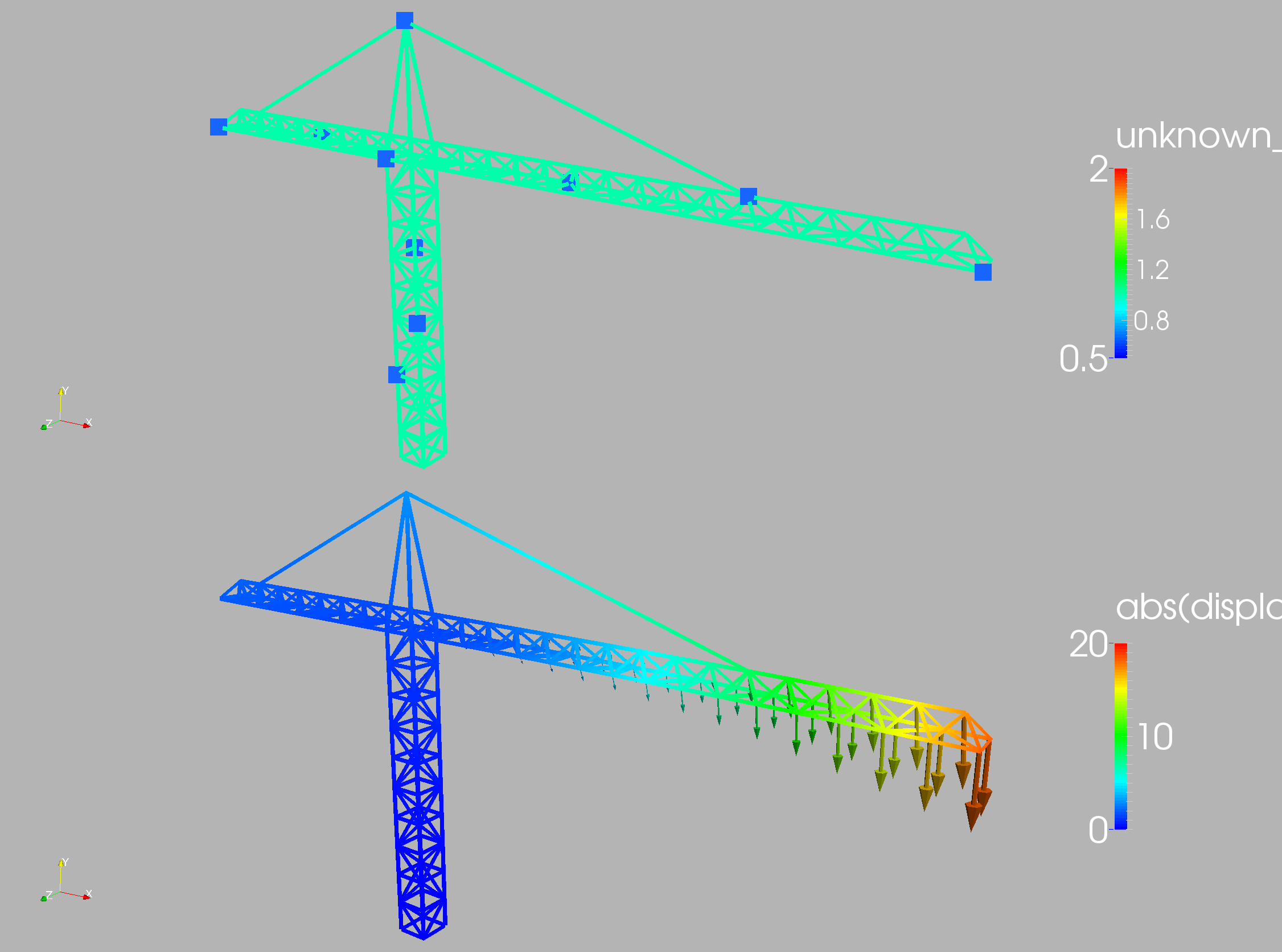
Figure 6.1. Crane: base case ($\alpha=1.0$)

The case is shown in Figure 6.1 and considers a typical crane used at construction sites. The crane has a height of 1,400 cm, and the arm has a length of 2,500 cm. A typical truss is about 100 cm long and has an area of 5 sqcm. Density, Young’s modulus and Poisson rate were set to $\rho=7.8,E=2\cdot 10^{12},\nu=0.3$ respectively (all cgs units). The two end points on the arm had loads of $f_{y}=-2.0\cdot 10^{9}~{}gr~{}cm/sec^{2}$ applied, while the two end points on balancing/back part of the arm had loads of $f_{y}=-1.0\cdot 10^{9}~{}gr~{}cm/sec^{2}$. The finite element discretization consisted of 350 linear truss elements. The loads lead to a deformation in the vertical direction $w_{y}=-18~{}cm$ at the tip of the arm. The top figure shows the strength factor $\alpha$ and the ten measuring points used (which in this case coincide with nodes of the finite element mesh), while the bottom figure displays the deformation field.

Displacement Measurements

Given the desired/measured displacements at these 10 measuring points, different starting values for the strength factor $\alpha$ were explored. Figures 6.2-6.4 show the results obtained when starting from a uniform value of $\alpha=2.0$ without Figure 6.3 and with Figure 6.4 gradient smoothing. One can see that for this case gradient smoothing is essential.

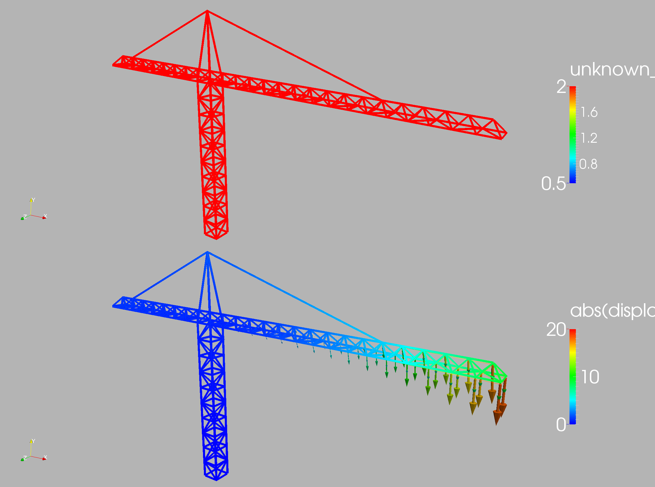
Figure 6.2. Crane: Start: $\alpha=2.0$, Iteration: 0

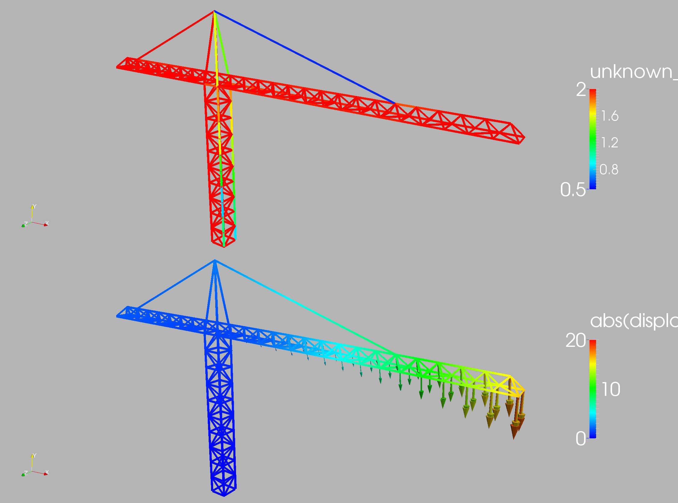
Figure 6.3. Crane: Start: $\alpha=2.0$, Iteration: 90, No Smoothing of Gradients

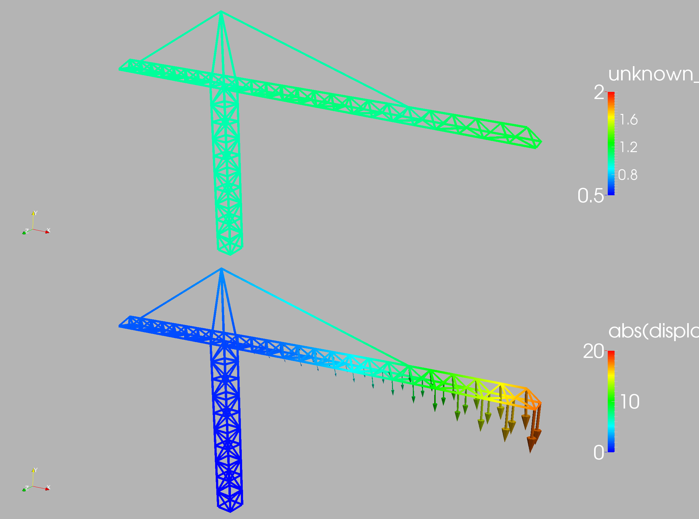
Figure 6.4. Crane: Start: $\alpha=2.0$, Iteration: 90, Smoothing of Gradients

Figures 6.5, 6.6 and 6.7 show the results obtained when starting from a random distribution of $\alpha$ without and with gradient smoothing. As before, one can see that for this case gradient smoothing is essential.

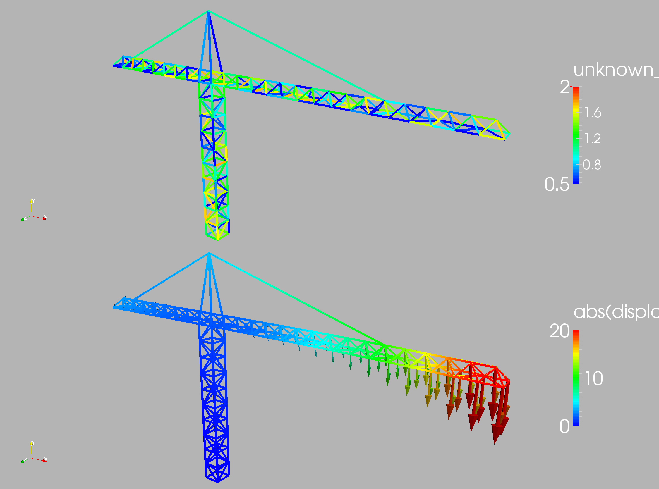
Figure 6.5. Crane: Start: Random $\alpha$, Iteration: 0

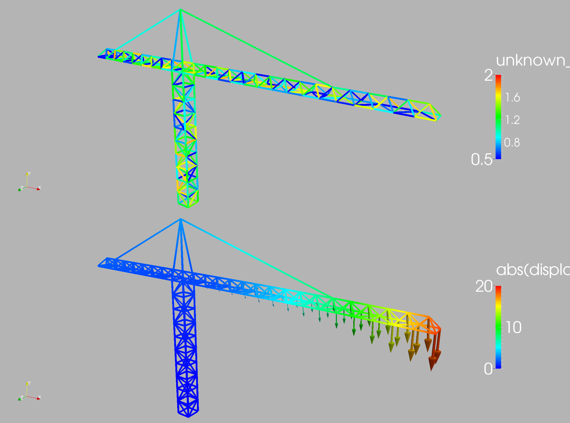
Figure 6.6. Crane: Start: Random $\alpha$, Iteration: 90, No Smoothing of Gradients

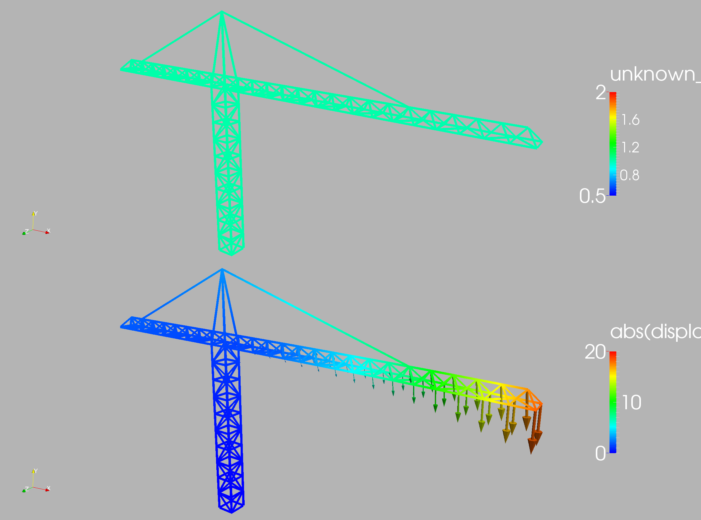
Figure 6.7. Crane: Start: Random $\alpha$, Iteration: 90, Smoothing of Gradients

Strain Measurements

Ten strain measuring points were defined in trusses along the structure (see top left of Figures 6.8, 6.9 and 6.10). Given the desired/measured strains at these 10 measuring points, different starting values for the strength factor $\alpha$ were explored. The results obtained and behaviours observed were very similar to the cases with displacement measurements: gradient smoothing was essential. Therefore, gradient smoothing has always been applied for all the results shown in the sequel. Figures 6.8, 6.9 and 6.10 show the results obtained when starting from a uniform value of $\alpha=0.5$. The top figures show the actual values while the bottom part shows the expected strain and strength distribution in the trusses. Note also on the top left the differences in target and actual strain at the measurement points.

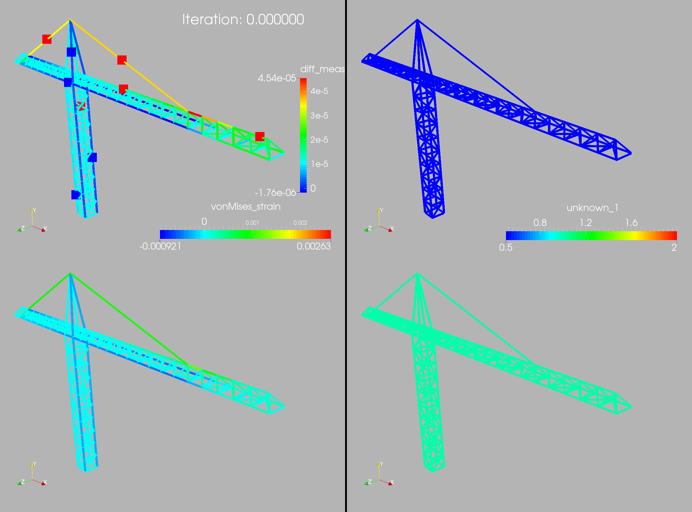
Figure 6.8. Crane: Start: $\alpha=0.5$, Iteration: 0

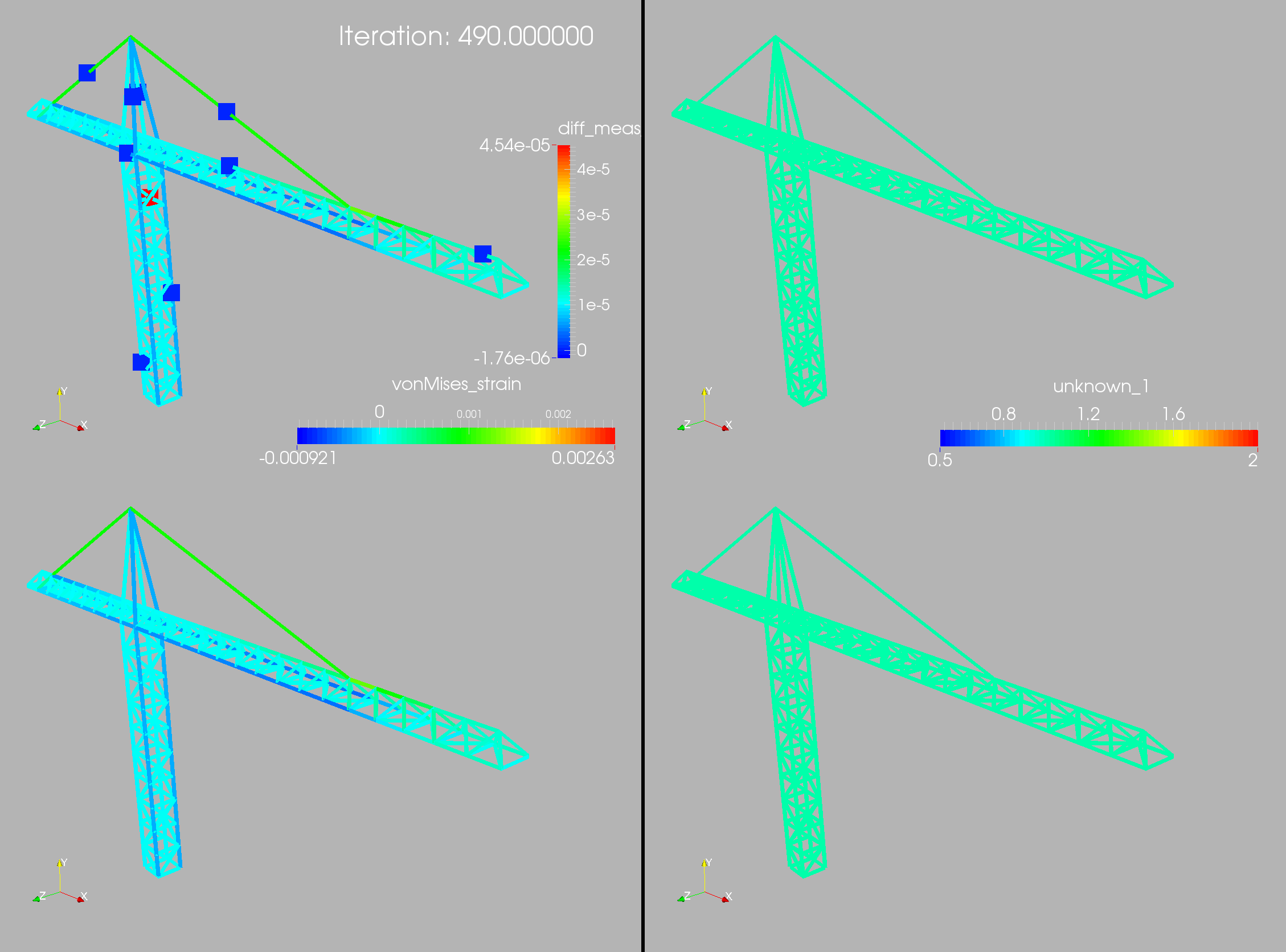
Figure 6.9. Crane: Start: $\alpha=0.5$, Iteration: 490

Figure 6.10. Crane: Start: $\alpha=0.5$, abs(Minimum) and Maximum

Figures 6.11, 6.12 and 6.13 show the results obtained when starting from a uniform value of $\alpha=1.0$ for the case that the lower part of the crane tower has been weakened to $\alpha=0.5$. As before, the top figures show the actual values while the bottom part shows the expected strain and strength distribution in the trusses.

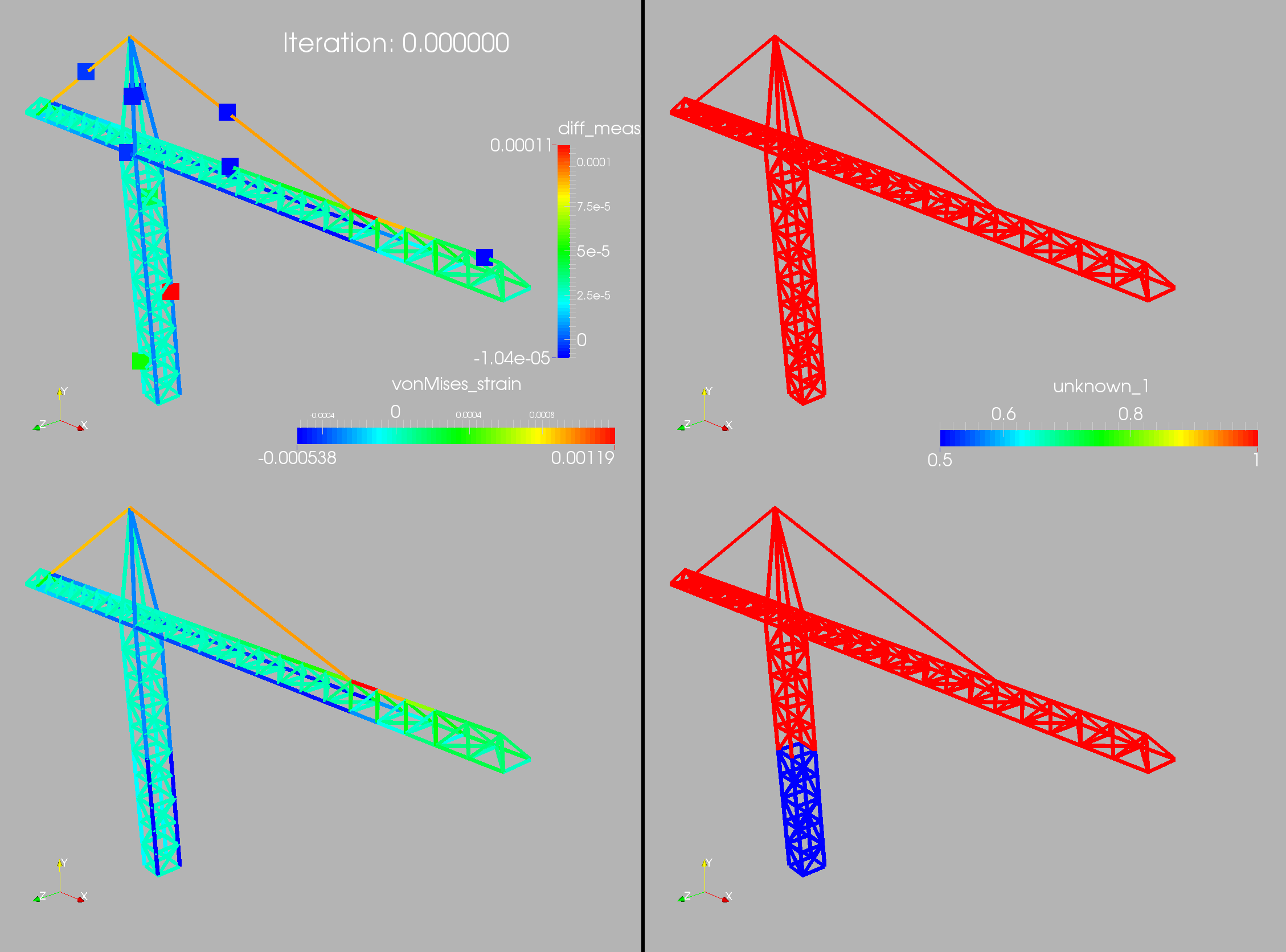
Figure 6.11. Weakened Crane: Start: $\alpha=1.0$, Iteration: 0

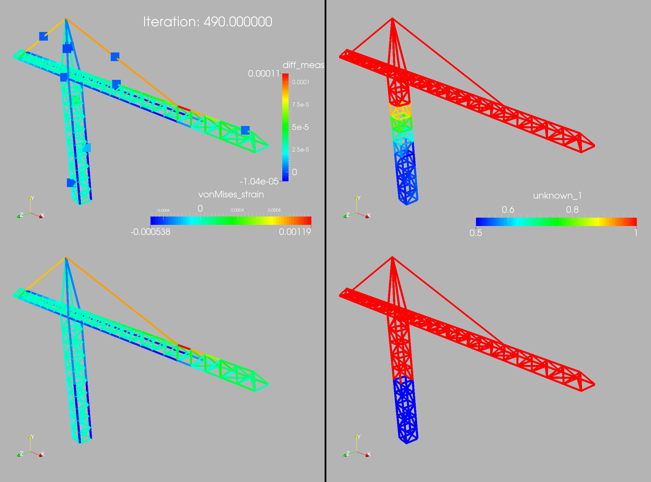
Figure 6.12. Weakened Crane: Start: $\alpha=1.0$, Iteration: 490

Figure 6.13. Weakened Crane: Start: $\alpha=1.0$, abs(Minimum) and Maximum

Displacement Measurements With Multiple Loads

The same ‘weakened bottom’ scenario was also computed for the 10 displacement measurement points shown before, but with 3 load scenarios. The first is the same as before, the second induces a torsion of the mast and the third applies forces between the mast and the end of the arm. Figures 6.14, 6.15 and 6.16 show the results obtained when starting from a uniform value of $\alpha=1.0$. In the figures, the top left shows the computed strength factor, the top right the desired (exact) strength factor, while the bottom shows the displacements (computed and desired overlapped) for the 3 load cases.

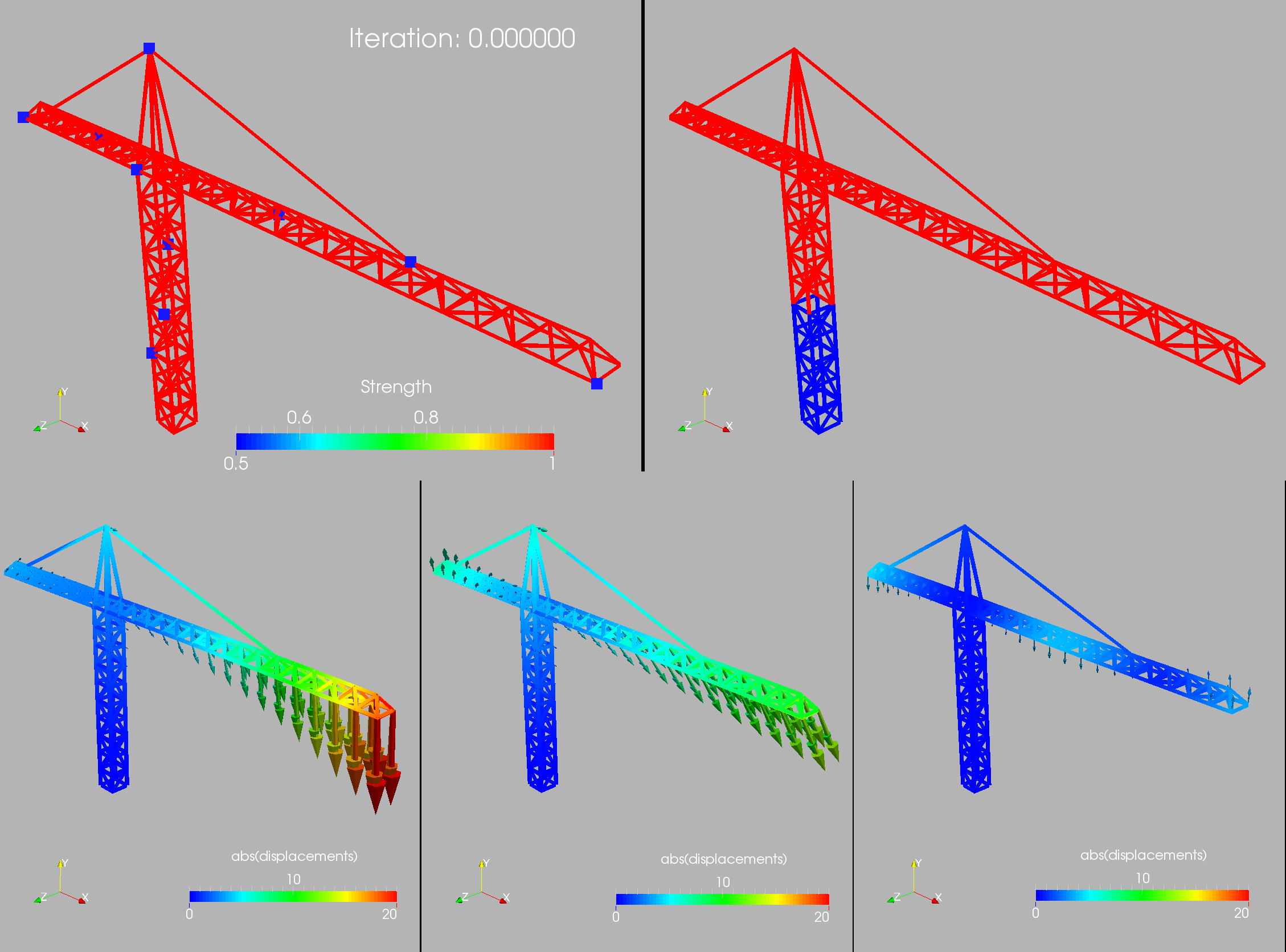
Figure 6.14. Weakened Crane: Start: $\alpha=1.0$, Iteration: 0

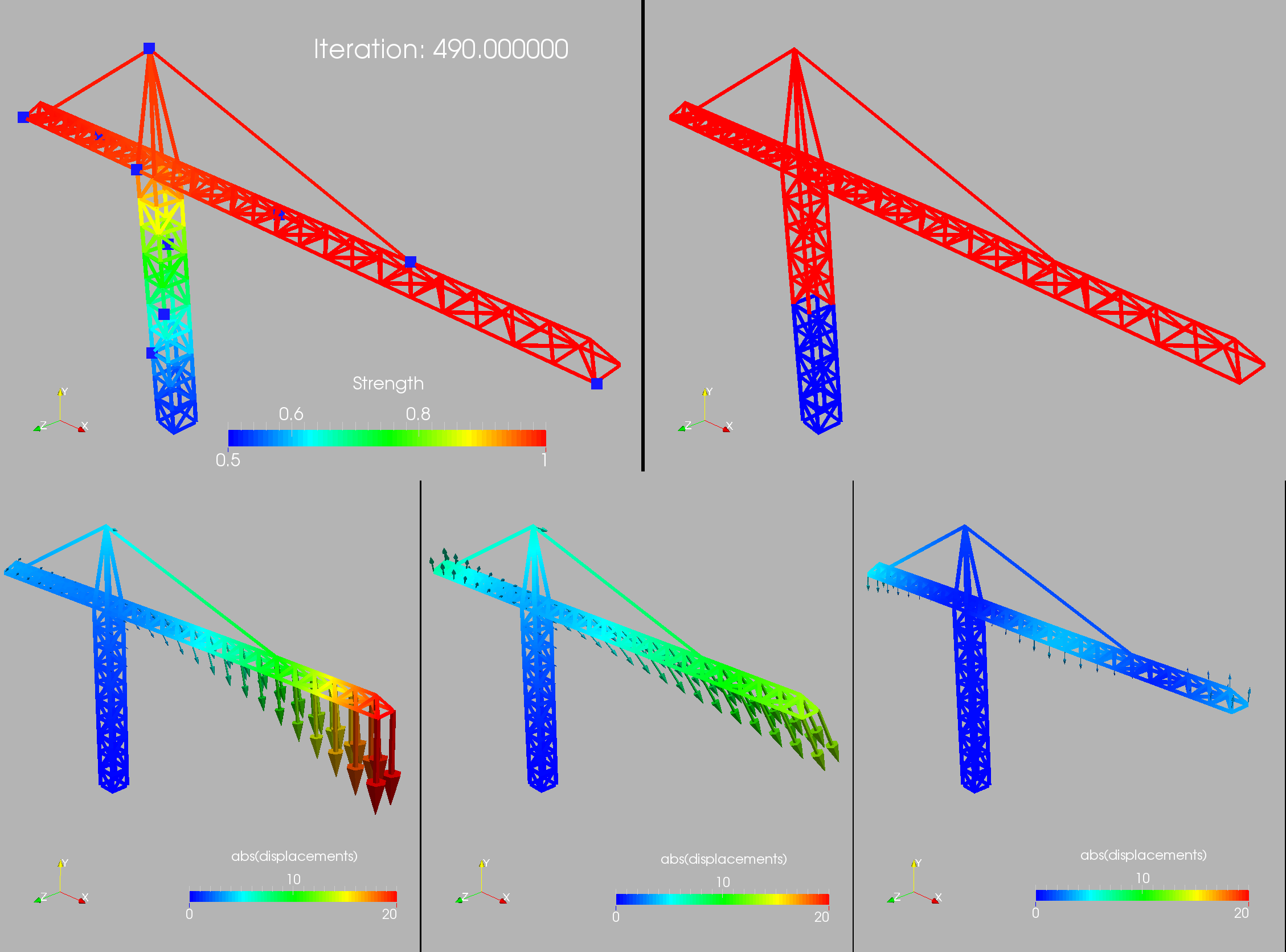
Figure 6.15. Weakened Crane: Start: $\alpha=1.0$, Iteration: 490

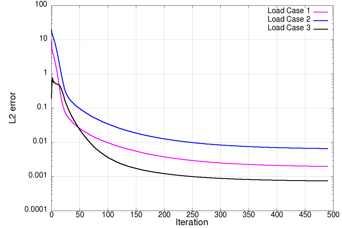
Figure 6.16. Weakened Crane: Convergence History for the Load Cases

6.2. Footbridge

This case considers a typical footbridge and was taken from [13]. The forces and material number of the trusses, whose dimensions (all units in mks) have been compiled in Table 6.1, can be discerned from Figure 6.17. Density, Young’s modulus and Poisson rate were set to $\rho=7,800,E=2\cdot 10^{11},\nu=0.3$ respectively.

Material #	Properties. Dimensions in mm
1	Steel plate. $t=10$
2	Steel beam. Hollow section $300\times 200\times 12$
3	Steel beam. Hollow section $200\times 200\times 10$
4	Steel beam. Hollow section $180\times 180\times 10$
5	Steel beam. Hollow section $180\times 180\times 5$
6	Steel beam. Hollow section $200\times 200\times 10$
7	Steel beam. Hollow section $200\times 100\times 5$

Table 6.1. Materials and dimensions of plates and beams.

The structure was modeled using 136 shell and 329 beam elements. The bridge is under a distributed load of $1$ MPa on the downwards direction, applied to every plate, as well as gravity. Figure 6.18 shows the target case where we have $E=0.1E_{0}$ at one beams in the structure. In 6.18(a), the location of the 8 sensors is shown, along with the target displacements. Starting from a uniform value of $\alpha=1.0$, shown in Figure 6.19, the target case is nearly reproduced in 200 steepest descent iterations, as can be seen in Figure 6.20. The evolution of the objective function is shown in figure 6.21.

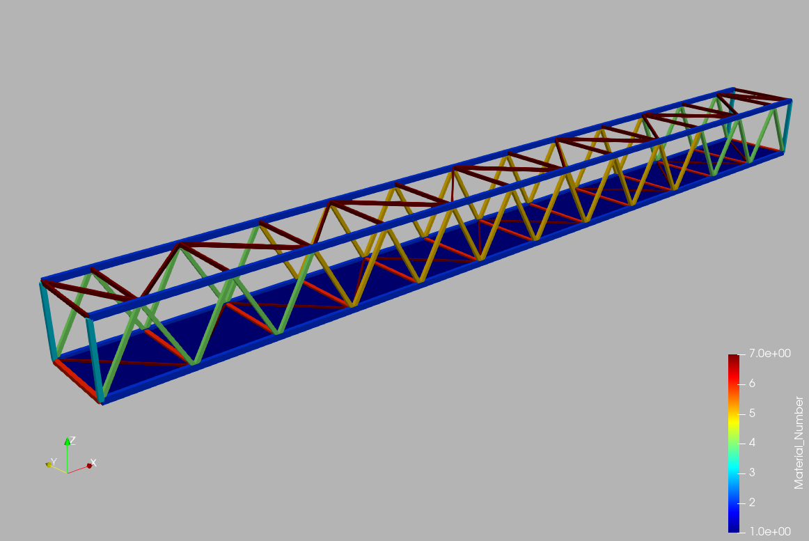
Figure 6.17. Footbridge: materials

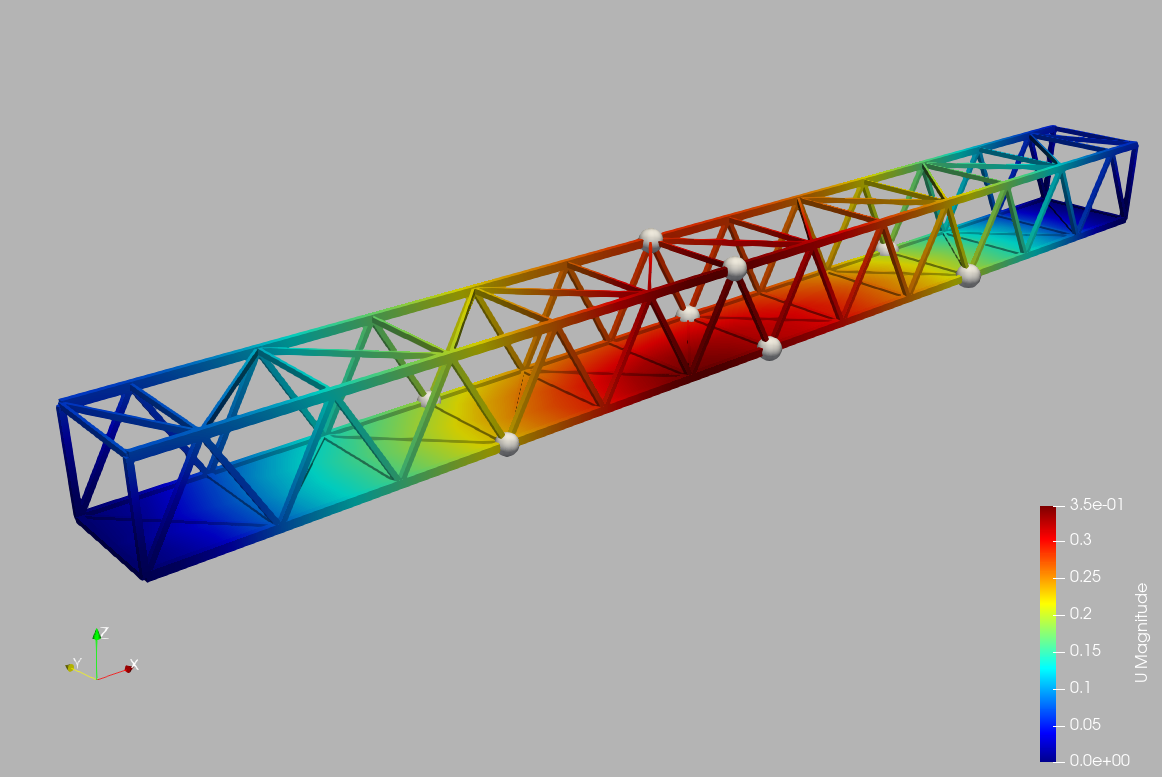
(a) Target displacements and sensor locations

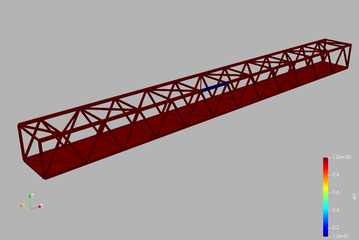
(b) Target strength factor

Figure 6.18. Footbridge: Target conditions

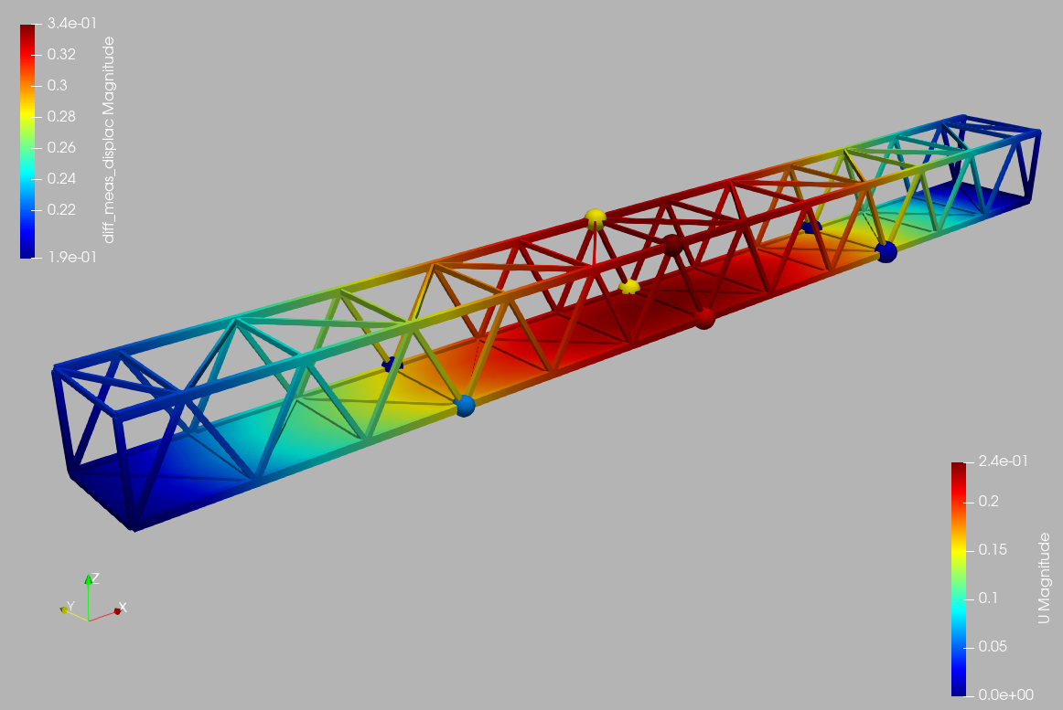
(a) Initial displacements and sensor values

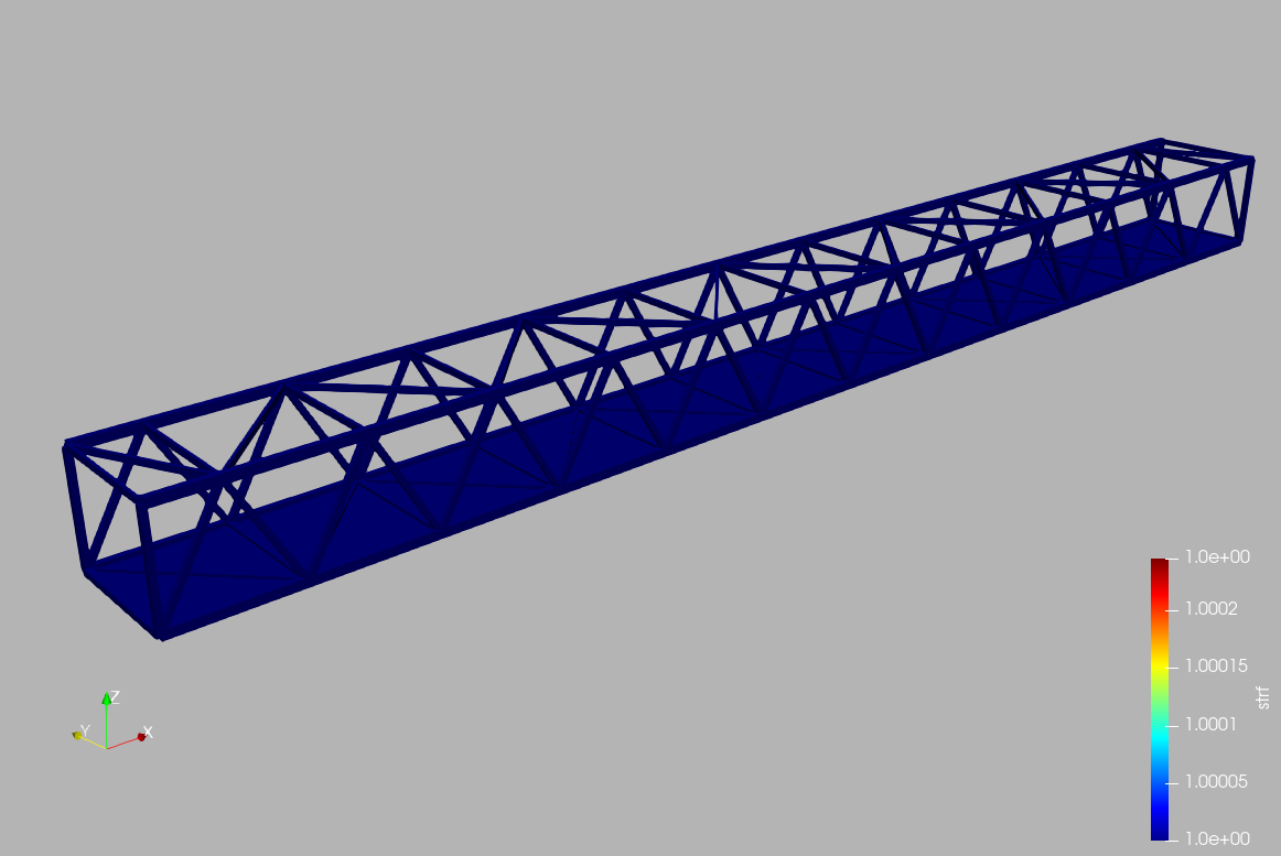
(b) Initial strength factor

Figure 6.19. Footbridge: Initial conditions

(a) Displacements obtained

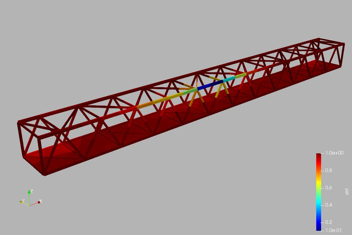
(b) Strength factor obtained

Figure 6.20. Footbridge: Solution obtained

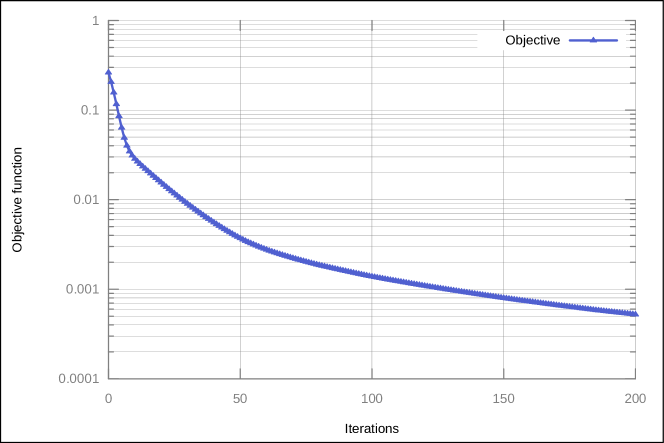
Figure 6.21. Footbridge: Objective function history

6.3. Plate with Hole

The case is shown in Figures 6.22, 6.23 and 6.24 and considers a plate with a hole. The plate dimensions are (all units in mks): $0\leq x\leq 60$, $0\leq y\leq 30$, $0\leq z\leq 0.1$. A hole of diameter $d=10$ is placed in the middle ($x=30,y=15$). Density, Young’s modulus and Poisson rate were set to $\rho=7,800,E=2\cdot 10^{11},\nu=0.3$ respectively. 672 linear, triangular, plain stress elements were used. The left boundary of the plate is assumed clamped (${\bf u}=0$), while a horizontal load of $q_{x}=10^{5}$ was prescribed at the right end. The left part of the figures show the computed strength factor and displacements, while the right part displays the expected values (the strength factor range is $0.1\leq\alpha\leq 1$). The 14 measurement points, together with the differences in displacements between measured and computed values are also shown in the bottom right part.

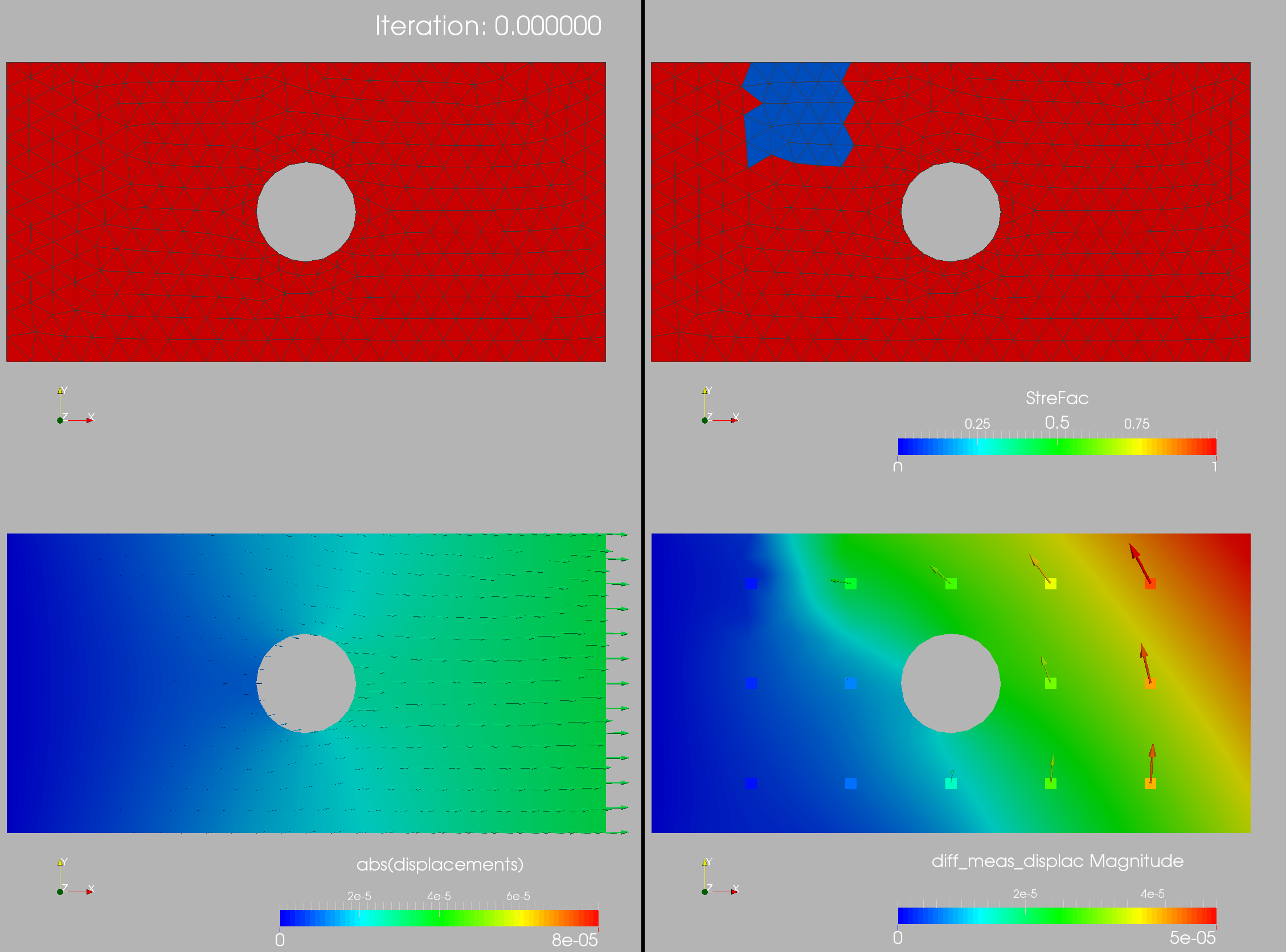
Figure 6.22. Plate With Hole: Start: $\alpha=1.0$, Iteration: 0

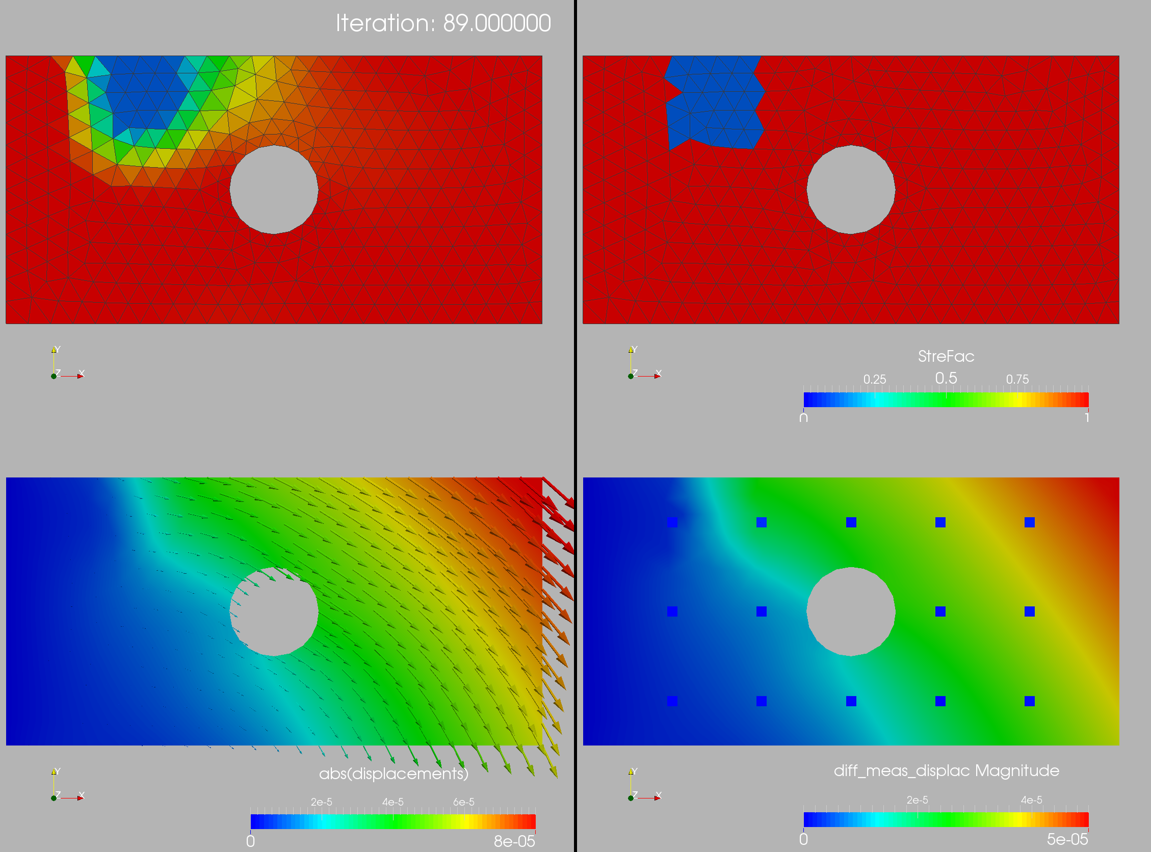
Figure 6.23. Plate With Hole: Start: $\alpha=1.0$, Iteration: 89

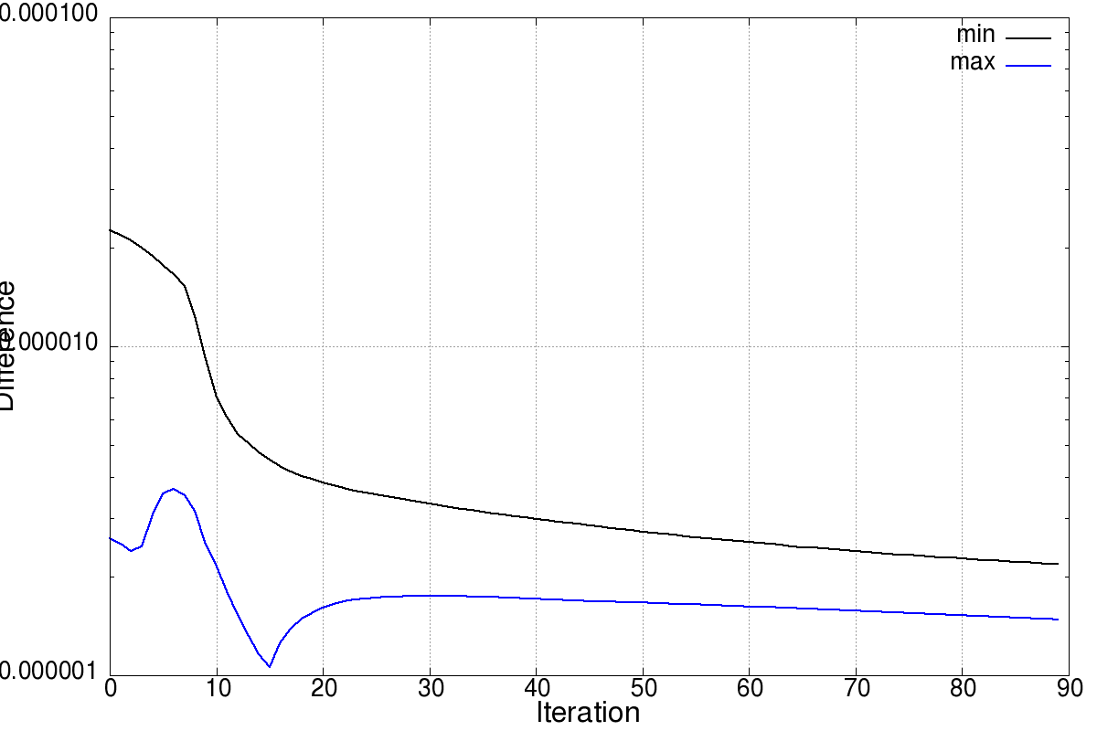
Figure 6.24. Plate With Hole: Start: $\alpha=1.0$, abs(Minimum) and Maximum

6.4. L-Shape

The case, taken from [10] is shown in Figures 6.25, 6.26 and 6.27 and considers an L-shaped block subjected to a vertical force. The plate dimensions are (all units in mks): $0\leq x\leq 0.6$, $0\leq y\leq 1.3$, $0\leq z\leq 0.30$. The upper part extends up to $x=0.45$, and the L-part extends to $y=0.3$. A fillet with radius $r=0.05$ was added to avoid extreme stress concentrations. Density, Young’s modulus and Poisson rate were set to $\rho=7,800,E=2\cdot 10^{11},\nu=0.3$ respectively. 14,622 linear, tetrahedral elements were used. The top boundary of the block is assumed clamped (${\bf u}=0$), while a vertical surface load of $f_{y}=-2\cdot 10^{7}$ was prescribed at the top of the L-shaped region (only the straight section, i.e. not the fillet).

The 10 visible measurement points (the other 10 are at the same $x,y$ positions but on the other $z$-face), together with the target displacements and strength factors are shown in figure 6.25 (the strength factor range again is $0.1\leq\alpha\leq 1$). . This case was particularly challenging because the weakened region does not have a considerable influence on the displacements. Therefore, many possible strength factor distributions can yield similar displacements. The smoothing of the gradient was a key tool for the optimizer to arrive at the proper solution.

Figure 6.26 shows the initial conditions for the optimization loop. The results obtained after 100 steepest descent iterations are displayed in figure 6.27. Note that 5 passes of gradient smoothing were employed. The evolution of the objective function is shown in figure 6.28.

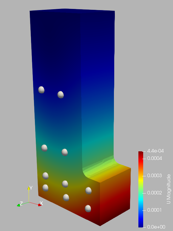
(a) Target displacements and sensor locations

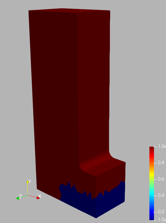
(b) Target strength factor

Figure 6.25. L-Shape: Target conditions

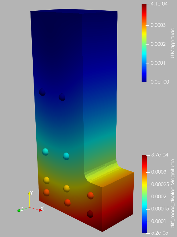
(a) Initial displacements and sensor locations

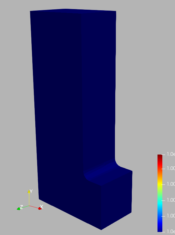
(b) Initial strength factor

Figure 6.26. L-Shape: Initial conditions

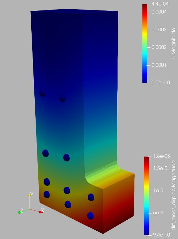
(a) Displacements obtained

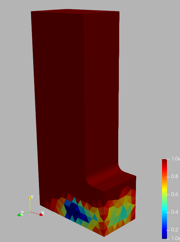
(b) Strength factor obtained

Figure 6.27. L-Shape: Solution obtained

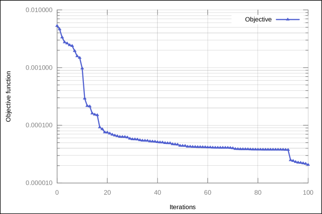
Figure 6.28. L-Shape: Objective function history

7. Conclusions and outlook

An adjoint-based procedure to determine weaknesses, or, more generally the material properties of structures has been presented. Given a series of force and deformation/strain measurements, the material properties are obtained by minimizing the weighted differences between the measured and computed values. It was found that in order to obtain reliable, convergent results the gradient of the cost function has to be smoothed.

Several examples are included that show the viability, accuracy and efficiency of the proposed methodology using both displacement and strain measurements.

We consider this a first step that demonstrates the viability of the adjoint-based methodology for system identification and its use for digital twins [20, 8]. Many questions remain open, of which we just mention two obvious ones:

• What sensor resolution is required to obtain reliable results ?

• Will these techniques work under uncertain measurements ? [2, 3].

Furthermore, the steepest descent procedures may be improved by going to a quasi or full Newton solver. But: will they be faster ?

The answers to these questions are currently under investigation.

8. Acknowledgements

This work is partially supported by NSF grant DMS-2110263 and the AirForce Office of Scientific Research under Award NO: FA9550-22-1-0248.

References

- [1] Nizar Faisal Alkayem, Maosen Cao, Yufeng Zhang, Mahmoud Bayat, and Zhongqing Su. Structural damage detection using finite element model updating with evolutionary algorithms: a survey. Neural Computing and Applications, 30:389–411, 2018.
- [2] Harbir Antil, Sergey Dolgov, and Akwum Onwunta. Ttrisk: Tensor train decomposition algorithm for risk averse optimization. Numerical Linear Algebra with Applications, n/a(n/a):e2481.
- [3] Harbir Antil, Sergey Dolgov, and Akwum Onwunta. State-constrained optimization problems under uncertainty: A tensor train approach. arXiv preprint arXiv:2301.08684, 2023.
- [4] Harbir Antil, Drew P Kouri, Martin-D Lacasse, and Denis Ridzal. Frontiers in PDE-constrained Optimization, volume 163. Springer, 2018.
- [5] Thomas Borrvall and Joakim Petersson. Topology optimization of fluids in stokes flow. International journal for numerical methods in fluids, 41(1):77–107, 2003.
- [6] M. Botz, A. Emiroglu, K. Osterminski, M. Raith, R. Wc̈hner, and C. Grosse. überwachung und modellierung der tragstruktur von windenergieanlagen. Beton- und Stahlbetonbau, 41:342–354, 2020.
- [7] Peter Cawley and Robert Darius Adams. The location of defects in structures from measurements of natural frequencies. The Journal of Strain Analysis for Engineering Design, 14(2):49–57, 1979.
- [8] Francisco Chinesta, Elias Cueto, Emmanuelle Abisset-Chavanne, Jean Louis Duval, and Fouad El Khaldi. Virtual, digital and hybrid twins: a new paradigm in data-based engineering and engineered data. Archives of computational methods in engineering, 27:105–134, 2020.
- [9] Guido Dhondt. Calculix user’s manual version 2.20. Munich, Germany, 2022.
- [10] Daniele Di Lorenzo, Victor Champaney, Claudia Germoso, Elias Cueto, and Francisco Chinesta. Data completion, model correction and enrichment based on sparse identification and data assimilation. Applied Sciences, 12(15):7458, 2022.
- [11] S. Grabke, K.-U. Bletzinger, and R. Wüchner. Development of a finite element-based damage localization technique for concrete by applying coda wave interferometry. Engineering Structures, 269:114585, 2022.
- [12] S. Grabke, F. Clauss, K.-U. Bletzinger, M. A. Ahrens, P. Mark, and R. Wüchner. Damage detection at a reinforced concrete specimen with coda wave interferometry. Materials, 14:5013, 2021.
- [13] Artūras Kilikevičius, Darius Bačinskas, Jaroslaw Selech, Jonas Matijošius, Kristina Kilikevičienė, Darius Vainorius, Dariusz Ulbrich, and Dawid Romek. The influence of different loads on the footbridge dynamic parameters. Symmetry, 12(4):657, 2020.
- [14] Hansang Kim and Hani Melhem. Damage detection of structures by wavelet analysis. Engineering structures, 26(3):347–362, 2004.
- [15] Boyan Stefanov Lazarov and Ole Sigmund. Filters in topology optimization based on helmholtz-type differential equations. International Journal for Numerical Methods in Engineering, 86(6):765–781, 2011.
- [16] Rainald Löhner. Applied computational fluid dynamics techniques: an introduction based on finite element methods. John Wiley & Sons, 2008.
- [17] Rainald Löhner. Feelast user’s manual. Fairfax, Virginia, 2023.
- [18] Rainald Löhner and Harbir Antil. Determination of volumetric material data from boundary measurements: Revisiting calderon’s problem. International Journal of Numerical Methods for Heat & Fluid Flow, 2020.
- [19] NMM Maia, JMM Silva, and RPC Sampaio. Localization of damage using curvature of the frequency-response-functions. In Proceedings of the 15th international modal analysis conference, volume 3089, page 942, 1997.
- [20] Laura Mainini and Karen Willcox. Surrogate modeling approach to support real-time structural assessment and decision making. AIAA Journal, 53(6):1612–1626, 2015.
- [21] SC Mohan, Dipak Kumar Maiti, and Damodar Maity. Structural damage assessment using frf employing particle swarm optimization. Applied Mathematics and Computation, 219(20):10387–10400, 2013.
- [22] Thomas Planès and Eric Larose. A review of ultrasonic coda wave interferometry in concrete. Cement and Concrete Research, 53:248–255, 2013.
- [23] Magdalena Rucka and Krzysztof Wilde. Application of continuous wavelet transform in vibration based damage detection method for beams and plates. Journal of sound and vibration, 297(3-5):536–550, 2006.
- [24] Maher Salloum and David B Robinson. Optimization of flow in additively manufactured porous columns with graded permeability. AIChE Journal, 68(9):e17756, 2022.
- [25] Juan C Simo and Thomas JR Hughes. Computational inelasticity, volume 7. Springer Science & Business Media, 2006.
- [26] Fredi Tröltzsch. Optimal control of partial differential equations: theory, methods, and applications, volume 112. American Mathematical Soc., 2010.
- [27] Olek C Zienkiewicz, Robert Leroy Taylor, and Jian Z Zhu. The finite element method: its basis and fundamentals. Elsevier, 2005.