A link between Kendall’s $\tau$, the length measure and the surface of bivariate copulas, and a consequence to copulas with self-similar support

Abstract

Working with shuffles we establish a close link between Kendall’s $\tau$, the so-called length measure, and the surface area of bivariate copulas and derive some consequences. While it is well-known that Spearman’s $\rho$ of a bivariate copula $A$ is a rescaled version of the volume of the area under the graph of $A$, in this contribution we show that the other famous concordance measure, Kendall’s $\tau$, allows for a simple geometric interpretation as well - it is inextricably linked to the surface area of $A$.

1 Introduction

Spearman’s $\rho$ of a bivariate copula $A$ is a rescaled version of the volume below the graph of $A$ (see [3, 11]) in the sense that

$$\rho(A)=12\int_{[0,1]^{2}}A\,d\lambda_{2}-3$$

holds. Letting $[A]_{t}:=\{(x,y)\in[0,1]^{2}:A(x,y)\geq t\}$ denote the lower $t$-cut of $A$ for every $t\in[0,1]$ and applying Fubini’s theorem directly yields

$$\rho(A)=12\int_{[0,1]}\lambda_{2}([A]_{t})d\lambda(t)-3,$$

which lead the authors of [1] to conjecturing that adequately rescaling the so-called length measure $\ell(A)$ of $A$, defined as the average arc-length of the contour lines of $A$, might result in a (new or already known) concordance measure. The conjecture was falsified in [1], only some but not all properties of a concordance measure are fulfilled, in particular, we do not have continuity with respect to pointwise convergence of copulas in general.

Motivated by the afore-mentioned facts, the objective of this note is two-fold: we first derive the somewhat surprising result that on a subfamily of bivariate copulas - the class $\mathcal{C}_{mcd}$ of all mutually completely dependent copulas (including all classical shuffles) - which is dense in the class $\mathcal{C}$ of all bivariate copulas with respect to uniform convergence, the length measure is, in fact, an affine transformation of Kendall’s $\tau$ and vice versa. As a consequence, the length measure restricted to $\mathcal{C}_{mcd}$ is continuous with respect to pointwise convergence of copulas. We then focus on the surface area of bivariate copulas and derive analogous statements, i.e., that on the class $\mathcal{C}_{mcd}$ the surface area is an affine transformation of Kendall’s $\tau$ (and hence of the length measure) too. For obtaining both main results a simple geometric identity linking the length measure and the surface area with the area of the set $\Omega_{\sqrt{2}}$, given by

$$\Omega^{A_{h}}_{\sqrt{2}}=\left\{(x,y)\in[0,1]^{2}:h(x)\leq y,\,h^{-1}(y)\leq x\right\},$$ (1)

where $h$ denotes the transformation corresponding to the completely dependent copula $A_{h}$, will be key. An application to calculating Kendall’s $\tau$, the length measure and the surface area of completely dependent copulas with self-similar support concludes the paper.

2 Notation and preliminaries

In the sequel we will let $\mathcal{C}$ denote the family of all bivariate copulas. For each copula $C\in\mathcal{C}$ the corresponding doubly stochastic measure will be denoted by $\mu_{C}$, i.e., $\mu_{C}([0,x]\times[0,y])=C(x,y)$ holds for all $x,y\in[0,1]$. Considering the uniform metric $d_{\infty}$ on $\mathcal{C}$ it is well-known that $(\mathcal{C},d_{\infty})$ is a compact metric space and that in $\mathcal{C}^{d}$ pointwise and uniform convergence are equivalent. For more background on copulas and doubly stochastic measures we refer to [3, 11].
For every metric space $(\Omega,d)$ the Borel $\sigma$-field in $\Omega$ will be denoted by $\mathcal{B}(\Omega)$. The Lebesgue measure on the Borel $\sigma$-field $\mathcal{B}([0,1]^{2})$ of $[0,1]^{2}$ will be denoted by $\lambda_{2}$, the univariate version on $\mathcal{B}([0,1])$ by $\lambda$. Given probability spaces $(\Omega,\mathcal{A},\mathbb{P})$ and $(\Omega^{\prime},\mathcal{A}^{\prime},\mathbb{P})^{\prime}$ and a measurable transformation $T:\Omega\rightarrow\Omega^{\prime}$ the push-forward of $\mathbb{P}$ via $T$ will be denoted by $\mathbb{P}^{T}$, i.e., $\mathbb{P}^{T}(F)=\mathbb{P}(T^{-1}(F))$ for all $F\in\mathcal{A}^{\prime}$.
In what follows, Markov kernels will be a handy tool. A mapping $K\colon\mathbb{R}\times\mathcal{B}(\mathbb{R})\to[0,1]$ is called a Markov kernel from $(\mathbb{R},\mathcal{B}(\mathbb{R}))$ to $(\mathbb{R},\mathcal{B}(\mathbb{R}))$ if the mapping $x\mapsto K(x,B)$ is measurable for every fixed $B\in\mathcal{B}(\mathbb{R})$ and the mapping $B\mapsto K(x,B)$ is a probability measure for every fixed $x\in\mathbb{R}$. A Markov kernel $K\colon\mathbb{R}\times\mathcal{B}(\mathbb{R})\to[0,1]$ is called regular conditional distribution of a (real-valued) random variable $Y$ given (another random variable) $X$ if for every $B\in\mathcal{B}(\mathbb{R})$

$$K(X(\omega),B)=\mathbb{E}(\mathds{1}_{B}\circ Y|X)(\omega)$$

holds $\mathbb{P}$-a.s. It is well known that a regular conditional distribution of $Y$ given $X$ exists and is unique $\mathbb{P}^{X}$-almost surely. For every $A\in\mathcal{C}$ (a version of) the corresponding regular conditional distribution (i.e., the regular conditional distribution of $Y$ given $X$ in the case that $(X,Y)\sim A$) will be denoted by $K_{A}(\cdot,\cdot)$ and directly be interpreted as mapping from $K_{A}:\,[0,1]\times\mathcal{B}([0,1])\rightarrow[0,1]$. Note that for every $A\in\mathcal{C}$ and Borel sets $E,F\in\mathcal{B}([0,1])$ we have the following disintegration formulas:

$$\int_{E}K_{A}(x,F)d\lambda(x)=\mu_{A}(E\times F)\quad\text{ and }\quad\int_{[0,1]}K_{A}(x,F)d\lambda(x)=\lambda(F)$$ (2)

For more details and properties of conditional expectations and regular conditional distributions we refer to [8, 10].
A copula $A\in\mathcal{C}$ will be called completely dependent if there exists some $\lambda$-preserving transformation $h:[0,1]\rightarrow[0,1]$ (i.e., a transformation with $\lambda^{h}=\lambda$) such that $K(x,E)=\mathbf{1}_{E}(h(x))$ is a Markov kernel of $A$. The copula induced by $h$ will be denoted by $A_{h}$, the class of all completely dependent copulas by $\mathcal{C}_{cd}$. A completely dependent copula $A_{h}$ is called mutually completely dependent, if the transformation $h$ is bijective. Notice that in this case the transpose $A_{h}^{t}$ of $A_{h}$, defined by $A_{h}^{t}(x,y)=A_{h}(y,x)$, coincides with $A_{h^{-1}}$. The family of all mutually completely dependent copulas will be denoted by $\mathcal{C}_{mcd}$. It is well known (see [3, 11]) that $\mathcal{C}_{mcd}$ is dense in $(\mathcal{C},d_{\infty})$, in fact even the family of all equidistant even shuffles (again see [3, 11]) is dense. For further properties of completely dependent copulas we refer to [13] and the references therein.

Turning towards the length profile introduced and studied in [1], let $\Gamma_{A,t}$ denote the boundary of the lower $t$-cut $[A]_{t}$ in $(0,1)^{2}$ and $H_{1}(\Gamma_{A,t})$ it’s arc-length. Then the length profile of $A$ is defined as the function $L_{A}:[0,1]\rightarrow[0,\infty)$, given by

$$L_{A}(t)=H_{1}(\Gamma_{A,t}).$$ (3)

It is straightforward to show see that

$$\sqrt{2}(1-t)\leq L_{A}(t)\leq 2(1-t)$$

holds for every $t\in(0,1)$. Building upon $L_{A}$ the so-called length measure $\ell(A)$ of $A$ is defined as

$$\ell(A)=\int_{(0,1)}L_{A}(t)d\lambda(t)$$ (4)

and describes the average arc-length of upper $t$-cuts of $A$. It is straightforward to verify that

$$\ell(W)=\frac{1}{\sqrt{2}}\leq\ell(A)\leq 1=\ell(M)$$ (5)

as well as $\ell(A)\in[\frac{1}{\sqrt{2}},1]$ holds (ineq. (5) was also one of the reasons for falsely conjecturing that the length measure might be transformable into a concordance measure).

In [1] it was shown that for mutually completely dependent copulas $A_{h}$ the length profile allows for a simple calculation. In fact, using the co-area formula we have

$$\ell(A_{h})=\int_{(0,1)^{2}}\|\nabla A_{h}(u,v)\|_{2}\,d\lambda_{2}(u,v),$$

where $\nabla A_{h}$ denotes the gradient of $A_{h}$ (whose existence $\lambda_{2}$-almost everywhere is assured by Rademacher’s theorem and Lipschitz continuity, see [5]). The last equation simplifies to the nice identity

$$\ell(A_{h})=1-(2-\sqrt{2})\,\lambda_{2}(\Omega_{\sqrt{2}}),$$ (6)

with

$$\Omega_{\sqrt{2}}^{A_{h}}:=\Omega_{\sqrt{2}} = \left\{(u,v)\in(0,1)^{2}:\|\nabla A_{h}(u,v)\|_{2}=\sqrt{2}\right\}$$ (7)

$$= \left\{(u,v)\in(0,1)^{2}:h(u)\leq v,\,h^{-1}(v)\leq u\right\}$$

Throughout the rest of this note we will only write $\Omega_{\sqrt{2}}$ instead of $\Omega_{\sqrt{2}}^{A_{h}}$ whenever no confusion will arise. Notice that for classical equidistant straight shuffles eq. (6) implies that $\ell(A_{h})$ can be calculated by simply counting squares as Figure 2 illustrates in terms of two simple examples - one shuffle with three, and a second one with nice equidistant stripes.

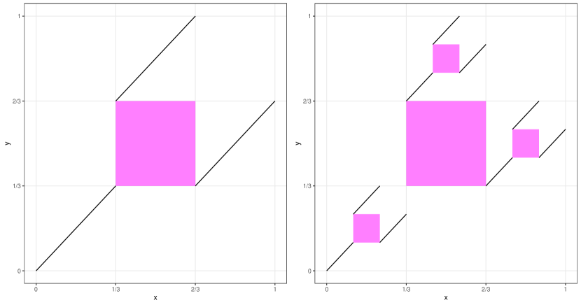
Figure 1: The set $\Omega_{\sqrt{2}}$ (in magenta) for an even shuffles of three strips (left panel) and nine strips (right panel). In this case we have $\lambda_{2}(\Omega_{\sqrt{2}})=\frac{1}{9}$ and $\ell(A_{h})=1-(2-\sqrt{2})\frac{1}{9}$ for the first shuffle and $\lambda_{2}(\Omega_{\sqrt{2}})=\frac{1}{9}+\frac{1}{27}$ as well as $\ell(A_{h})=1-(2-\sqrt{2})\left(\frac{1}{9}+\frac{1}{27}\right)$ for the second one.

3 The interrelations

We now derive a simple formula linking Kendall’s $\tau$ and the length measure for mutually completely dependent copula and start with some preliminary observations. Working with checkerboard copulas, using integration by parts (see [11]) and finally applying an approximation result like [9, Theorem 3.2] yields that for arbitrary bivariate copulas $A,B\in\mathcal{C}$ the following identity holds:

$$\tau(A)=4\int_{[0,1]^{2}}Ad\mu_{A}-1=4\left(\frac{1}{2}-\int_{[0,1]^{2}}K_{A}(x,[0,y])K_{A^{t}}(y,[0,x])d\lambda_{2}(x,y)\right)-1.$$ (8)

For $A_{h}\in\mathcal{C}_{mcd}$ eq. (8) can be derived in the following simple alternative way, which we include for the sake of completeness: Using the fact that for $A_{h}\in\mathcal{C}_{mcd}$ and every $x\in[0,1]$ we have

$$A(x,h(x)) = \int_{[0,x]}K_{A_{h}}(t,[0,h(x)])d\lambda(t)=\int_{[0,x]}K_{A_{h}}(t,[0,h(x)))d\lambda(t)$$

$$= \int_{[0,x]}\mathbf{1}_{[0,h(x))}(h(t))d\lambda(t)=\int_{[0,x]}(1-\mathbf{1}_{[h(x),1]}(h(t))d\lambda(t)$$

$$= x-\int_{[0,1]}\mathbf{1}_{[0,x]}(t)\mathbf{1}_{[h(x),1]}(h(t))d\lambda(t).$$

Using disintegration and change of coordinates directly yields

$$\int_{[0,1]^{2}}Ad\mu_{A} = \int_{[0,1]}A(x,h(x))d\lambda(x)=\frac{1}{2}-\int_{[0,1]}\int_{[0,1]}\mathbf{1}_{[0,x]}(t)\mathbf{1}_{[h(x),1]}(h(t))d\lambda(t)d\lambda(x)$$

and hence proves eq. (8). The latter identity, however, boils down to an affine transformation of $\lambda_{2}(\Omega_{\sqrt{2}})$ by considering

$$\int_{[0,1]^{2}}Ad\mu_{A} = \frac{1}{2}-\int_{[0,1]}\int_{[0,1]}\mathbf{1}_{[0,x]}(h^{-1}\circ h(t))\mathbf{1}_{[h(x),1]}(h(t))d\lambda(t)d\lambda(x)$$

$$= \frac{1}{2}-\int_{[0,1]}\int_{[0,1]}\mathbf{1}_{[0,x]}(h^{-1}(y))\mathbf{1}_{[h(x),1]}(y)d\lambda(y)d\lambda(x)$$

$$= \frac{1}{2}-\lambda_{2}(\Omega_{\sqrt{2}}).$$

Having this, the identity

$$\tau(A_{h})=4\left(\frac{1}{2}-\lambda_{2}(\Omega_{\sqrt{2}})\right)-1=1-4\lambda_{2}(\Omega_{\sqrt{2}}).$$ (9)

follows immediately. Notice that eq. (9) implies that the area of $\Omega_{\sqrt{2}}$ coincides with the quantity inv(h) as studied in [12, Lemma 3.1]. Comparing eq. (6) and eq. (9) shows the existence of an affine transformation $a:[-1,1]\rightarrow[\frac{1}{\sqrt{2}},1]$ such that

$$a\left(\tau(A_{h})\right)=\ell(A_{h})$$

holds for every $A_{h}\in\mathcal{C}_{mcd}$ - in other words, we have proved the subsequent result:

Theorem 3.1.

For every $A_{h}\in\mathcal{C}_{mcd}$ the following identity linking the length measure $\ell$ and Kendall’s $\tau$ holds:

$$\ell(A_{h})=1-\frac{2-\sqrt{2}}{4}(1-\tau(A_{h}))$$ (10)

Theorem 3.1 provides an answer to the question posed in [1], ‘whether there are links between the length of level curves and concordance measures’ - even the conjectured ‘weighting’ mentioned in [1] is not necessary, in the class $\mathcal{C}_{mcd}$ all we need is a fixed affine transformation.

In [1] it was further shown that the length measure interpreted as function $\ell:\mathcal{C}\rightarrow[\frac{\sqrt{2}}{2},1]$ is not continuous w.r.t. $d_{\infty}$. The previous result implies, however, that within the dense subclass $\mathcal{C}_{mcd}$ the length measure is indeed continuous:

Corollary 3.2.

The mapping $\ell:\mathcal{C}_{mcd}\rightarrow[\frac{1}{\sqrt{2}},1]$ is continuous with respect to $d_{\infty}$.

Proof.

Suppose that $A_{h},A_{h_{1}},A_{h_{2}},\ldots$ are mutually completely dependent copulas and that the sequence $(A_{h_{n}})_{n\in\mathbb{N}}$ converges to $A_{h}$ pointwise. Being a concordance measure Kendall’s $\tau$ is continuous with respect to $d_{\infty}$, so we have $\lim_{n\rightarrow\infty}\tau(A_{h_{n}})=\tau(A_{h})$ and eq. (9) directly yields $\lim_{n\rightarrow\infty}\ell(A_{h_{n}})=\ell(A_{h})$. ∎

Corollary 3.3.

For every $z\in[\frac{1}{\sqrt{2}},1]$ there exists some mutually completely dependent copula $A_{h}$ with $\ell(A_{h})=z$. In other words, all values in $[\frac{1}{\sqrt{2}},1]$ are attained by $\ell$.

Proof.

According to [12] for each $(x,y)$ in the region determined by Kendall’ $\tau$ and Spearman’s $\rho$ there exists some mutually completely dependent copula $C_{h}$ fulfilling

$$(\tau(A_{h}),\rho(A_{h}))=(x,y).$$

Having this, the result directly follows via eq. (9). ∎

Moving away from the length measure we now turn to the surface area of copulas, derive analogous statements and start with showing yet another simple formula for elements in $\mathcal{C}_{mcd}$. Considering that copulas are Lipschitz continuous, the surface area $\textrm{surf}(A)$ of an arbitrary copula $A$ is given by

$$\textrm{surf}(A) = \int_{[0,1]^{2}}\sqrt{\left(\frac{\partial A}{\partial x}(x,y)\right)^{2}+\left(\frac{\partial A}{\partial y}(x,y)\right)^{2}+1}\,\,d\lambda_{2}(x,y)$$ (11)

$$= \int_{[0,1]^{2}}\sqrt{K_{A}(x,[0,y])^{2}+K_{A^{t}}(y,[0,x])^{2}+1}\,\,d\lambda_{2}(x,y).$$

Again working with mutually completely dependent copulas yields the following result:

Lemma 3.4.

For every $A_{h}\in\mathcal{C}_{mcd}$ the surface area of $A_{h}$ is given by

$$\textrm{surf}(A_{h})=\sqrt{2}-\left(2\sqrt{2}-1-\sqrt{3}\right)\lambda_{2}(\Omega_{\sqrt{2}}).$$ (12)

Proof.

For the case of a completely dependent copula $A_{h}$ eq. (11) obviously simplifies to

$$\textrm{surf}(A_{h}) = \int_{[0,1]^{2}}\sqrt{\mathbf{1}^{2}_{[0,y]}(h(x))+\mathbf{1}^{2}_{[0,x]}(h^{-1}(y))+1}\,\,d\lambda_{2}(x,y)$$

$$= \int_{[0,1]^{2}}\sqrt{\mathbf{1}_{[0,y]}(h(x))+\mathbf{1}_{[0,x]}(h^{-1}(y))+1}\,\,d\lambda_{2}(x,y).$$

Considering that the latter integrand is a step function only attaining the values $1,\sqrt{2}$ and $\sqrt{3}$, defining

$$\Omega_{0}^{A_{h}}:=\Omega_{0} = \left\{(x,y)\in(0,1)^{2}:h(x)>y,\,h^{-1}(y)>x\right\}$$

as well as ($\Omega_{\sqrt{2}}$ as before)

$$\Omega_{1}^{A_{h}}:=\Omega_{1} = [0,1]^{2}\setminus(\Omega_{\sqrt{2}}\cup\Omega_{0})$$

we therefore have

$$\textrm{surf}(A_{h}) = \lambda_{2}(\Omega_{0})+\sqrt{2}\,\lambda_{2}(\Omega_{1})+\sqrt{3}\,\lambda_{2}(\Omega_{\sqrt{2}}).$$

The latter identity can be further simplified: The measurable bijection $\Psi_{h}:[0,1]^{2}\rightarrow[0,1]^{2}$, defined by $\Psi_{h}(x,y)=(h^{-1}(y),h(x))$ obviously fulfills $\lambda_{2}^{\Psi_{h}}=\lambda_{2}$. Therefore using the fact that

$$\Psi_{h}^{-1}(\Omega_{0}) = \{(x,y)\in[0,1]^{2}:(h^{-1}(y),h(x))\in\Omega_{0}\}$$

$$= \{(x,y)\in[0,1]^{2}:h(x)\leq y,h^{-1}(y)\leq x\}=\Omega_{\sqrt{2}}$$

it follows that $\lambda_{2}(\Omega_{0})=\lambda_{2}(\Omega_{\sqrt{2}})$ holds. This altogether yields

$$\textrm{surf}(A_{h}) = \lambda_{2}(\Omega_{\sqrt{2}})+\sqrt{2}\,\lambda_{2}(\Omega_{1})+\sqrt{3}\,\lambda_{2}(\Omega_{\sqrt{2}})$$

$$= (1+\sqrt{3})\,\lambda_{2}(\Omega_{\sqrt{2}})+\sqrt{2}\left(1-2\lambda_{2}(\Omega_{\sqrt{2}})\right)$$

$$= \sqrt{2}+\underbrace{\left(1+\sqrt{3}-2\sqrt{2}\right)}_{<0}\,\lambda_{2}(\Omega_{\sqrt{2}}),$$

which completes the proof. ∎

Theorem 3.5.

For every $A_{h}\in\mathcal{C}_{mcd}$ the following identity linking the surface area and Kendall’s $\tau$ holds:

$$\textrm{surf}(A_{h})=\sqrt{2}-\frac{2\sqrt{2}-1-\sqrt{3}}{4}(1-\tau(A_{h}))$$ (13)

As in the case of the length measure we have the following two immediate corollaries:

Corollary 3.6.

The mapping $\textrm{surf}:\mathcal{C}_{mcd}\rightarrow[\frac{1+\sqrt{3}}{2},\sqrt{2}]$ is continuous with respect to $d_{\infty}$.

Corollary 3.7.

For every $z\in[\frac{1+\sqrt{3}}{2},\sqrt{2}]$ there exists some mutually completely copula $A_{h}$ with $\textrm{surf}(A_{h})=z$. In other words, all values in $[\frac{1+\sqrt{3}}{2},\sqrt{2}]$ are attained by surf.

Remark 3.8.

The afore-mentioned interrelations lead to the following seemingly new interpretation of the interplay between the two most well-known measures of concordance, Kendall’s $\tau$ and Spearman’s $\rho$, as studied in [3, 4, 12] (and the references therein): Within the dense class $\mathcal{C}_{mcd}$ maximizing/minimizing Kendall’s $\tau$ for a given value of Spearman’s $\rho$ is equivalent to maximizing/minimizing the surface area of copulas for a given value of the volume. Determining the exact $\tau$-$\rho$ region (for which according to [12] considering all shuffles is sufficient) is therefore reminiscent of the famous isoperimetric inequality bounding the surface area of a set by a function of the volume (see [6]).

4 Calculating $\tau,\ell$ and surf for mutually completely dependent copulas with self-similar support

We first recall the notion of so-called transformation matrices and the construction of copulas with fractal/self-similar support, then use these tools to construct mutually completely dependent copulas with self-similar support and finally derive simple expressions for Kendall’s $\tau$ and the length measure of copulas of this type.

Definition 4.1 ([7, 13, 14]).

An $n\times m$- matrix $T=(t_{ij})_{i=1\ldots n,\,j=1\ldots m}$ is called transformation matrix if it fulfills the following four conditions: (i) $\max(n,m)\geq 2$, (ii), all entries are non-negative, (iii) $\sum_{i,j}t_{ij}=1$, and (iv) no row or column has all entries $0$.

In other words, a transformation matrix is a probability distribution $\tau$ on $(\mathcal{I},2^{\mathcal{I}})$ with $\mathcal{I}=I_{1}\times I_{2}$, $I_{1}=\{1,\ldots,n\}$ and $I_{2}=\{1,\ldots,m\}$, such that $\tau(\{i\}\times I_{2})>0$ for every $i\in I_{1}$ and $\tau(I_{1}\times\{j\})>0$ for every $j\in I_{2}$.

Given a transformation matrix $T$ define the vectors $(a_{j})_{j=0}^{m},(b_{i})_{i=0}^{n}$ of cumulative column and row sums by

$$a_{0} = b_{0}=0$$

$$a_{j} = \sum_{j_{0}\leq j}\sum_{i=1}^{n}t_{ij}\hskip 14.22636ptj\in\{1,\ldots,m\}$$ (14)

$$b_{i} = \sum_{i_{0}\leq i}\sum_{j=1}^{m}t_{ij}\hskip 14.22636pti\in\{1,\ldots,n\}.$$

Considering that $T$ is a transformation matrix both $(a_{j})_{j=0}^{m}$ and $(b_{i})_{i=0}^{n}$ are strictly increasing. Consequently $R_{ji}:=[a_{j-1},a_{j}]\times[b_{i-1},b_{i}]$ are compact non-empty rectangles for every $j\in\{1,\ldots,m\}$ and $i\in\{1,\ldots,n\}$. Defining the contraction $w_{ji}:[0,1]^{2}\rightarrow R_{ji}$ by

$$w_{ji}(x,y)=\big{(}a_{j-1}+x(a_{j}-a_{j-1})\,,\,b_{i-1}+x(b_{i}-b_{i-1})\big{)}$$

therefore yields the IFSP $\{[0,1]^{2},(w_{ji})_{j=1\ldots m,i=1\ldots n},(t_{ij})_{j=1\ldots m,i=1\ldots n}\}$. The induced operator $V_{T}$ on $\mathcal{P}_{\mathcal{C}}$, given by

$$V_{T}(\mu):=\sum_{j=1}^{m}\sum_{i=1}^{n}t_{ij}\,\mu^{w_{ji}}$$ (15)

is easily verified to be well-defined (i.e., it maps $\mathcal{P}_{\mathcal{C}}$ into itself, again see [14, 7, 13]) - in the sequel we will therefore also consider $V_{T}$ as a transformation mapping $\mathcal{C}$ into itself. According to [13] for every transformation matrix $T$ there exists a unique copula $A_{T}^{*}$ with $V_{T}(A_{T}^{*})=A_{T}^{*}$ such that

$$\lim_{n\rightarrow\infty}D_{1}(V_{T}^{n}(B),A_{T}^{*})=0$$ (16)

holds for arbitrary $B\in\mathcal{C}$ (i.e., $A_{T}^{*}$ is the unique, globally attractive fixed point of $V_{T}$).

Suppose now that $2\leq N\in\mathbb{N}$ and let $\pi$ be a permutation of $\{1,\ldots,N\}$. Then the matrix $T_{\pi}=(t_{ij})_{i=1\ldots N,\,j=1\ldots N}$, defined by

$$t_{i,j}=\frac{1}{N}\,\mathbf{1}_{\{j\}}(\pi(i)),\quad i,j\in\{1,\ldots,N\}$$

is obviously a transformation matrix. To simplify notation we will simply write $V_{\pi}:=V_{T_{\pi}}$ as well as $A_{T_{\pi}}^{*}=A_{T}^{*}$ in the sequel. Obviously $V_{\pi}$ does not only map $\mathcal{C}$ to $\mathcal{C}$ but also $\mathcal{C}_{mcd}$ to $\mathcal{C}_{mcd}$. Considering that (see [13]) $\mathcal{C}_{cd}$ is closed in $(\mathcal{C},D_{1})$ using eq. (16) it follows immediately that $A_{\pi}^{*}\in\mathcal{C}_{mcd}$, so there exists some $\lambda$-preserving bijection $h_{\pi}^{*}$ with $A_{\pi}^{*}=A_{h^{*}}$. Since the support of $A_{\pi}^{*}$ is self-similar it seems intractable to calculate $\ell(A_{\pi}^{*}),\textrm{surf}(A_{\pi}^{*})$ and $\tau(A_{\pi}^{*})$ for general $\pi$. The results established in the previous section, however, make it possible to derive simple expressions for both quantities.

We start with a simple illustrative example and then prove the general result (in a different manner).

Example 4.2.

Consider $N=3$ and the permutation $\pi=(1,3,2)$. Since, firstly, $A_{\pi}^{*}\in\mathcal{C}_{mcd}$, secondly, $A_{\pi}^{*}$ is globally attractive, and since, thirdly, $\lim_{n\rightarrow\infty}\tau(V_{\pi}^{n}(M))=\tau(A_{\pi}^{*})$ implies $\lim_{n\rightarrow\infty}\lambda_{2}(\Omega_{\sqrt{2}}^{V_{\pi}^{n}(M)})=\lambda_{2}(\Omega_{\sqrt{2}}^{A_{\pi}^{*}})$, it suffices to calculate $\lambda_{2}\left(\Omega_{\sqrt{2}}^{A_{\pi^{*}}}\right)$ which can be done as follows: Obviously we have (see Figure 2 for an illustration of the steps 3-6 in the construction)

$$\lambda_{2}\left(\Omega_{\sqrt{2}}^{V_{\pi}(M)}\right) = \frac{1}{9}$$

$$\lambda_{2}\left(\Omega_{\sqrt{2}}^{V^{2}_{\pi}(M)}\right) = \frac{1}{9}+3\,\frac{1}{9^{2}}=\frac{1}{9}\left(1+\frac{1}{3}\right)$$

$$\lambda_{2}\left(\Omega_{\sqrt{2}}^{V^{3}_{\pi}(M)}\right) = \frac{1}{9}+3\,\frac{1}{9^{2}}+9\frac{1}{27^{2}}=\frac{1}{9}\left(1+\frac{1}{3}+\frac{1}{3^{2}}\right)$$

$$\vdots = \vdots$$

$$\lambda_{2}\left(\Omega_{\sqrt{2}}^{V^{n}_{\pi}(M)}\right) = \frac{1}{9}\left(1+\frac{1}{3}+\ldots+\frac{1}{3^{n-1}}\right)$$

which yields

$$\lambda_{2}\left(\Omega_{\sqrt{2}}^{A_{\pi^{*}}}\right)=\frac{1}{9}\frac{1}{1-\frac{1}{3}}=\frac{1}{6}.$$

Having that, using eqs. (6), (9) and (13) shows

$$\ell(A_{\pi}^{*})=1-(2-\sqrt{2})\frac{1}{6},\quad\tau(A_{\pi}^{*})=1-4\ \frac{1}{6}=\frac{1}{3}$$

as well as

$$\textrm{surf}(A_{\pi}^{*})=\sqrt{2}-\left(2\sqrt{2}-1-\sqrt{3}\right)\frac{1}{6}.$$

Figure 2: Supports of the copulas $V_{\pi}^{n}(M)$ (black line segments) and the corresponding sets $\Omega_{\sqrt{2}}^{V_{\pi}^{n}(M)}$ (magenta squares) for $n\in\{3,4,5,6\}$ and $\pi=(1,3,2)$ as considered in Example 4.2.

Theorem 4.3.

Suppose that $N\geq 2$ and that $\pi$ is a permutation of $\{1,\ldots,N\}$. Then the following identities hold for the copula $A_{\pi}^{*}$ with self-similar support:

$$\tau\left(A_{\pi}^{*}\right) = 1-4\,\frac{N}{N-1}\lambda_{2}\left(\Omega_{\sqrt{2}}^{V_{\pi}(M)}\right)$$

$$= 1-4\,\frac{1}{N(N-1)}\,\#\left\{(i,j)\in\{1,\ldots,N\}^{2}:\pi(i)<j\textrm{ and }\pi^{-1}(j)<i\right\}$$

$$\ell\left(A_{\pi}^{*}\right) = 1-(2-\sqrt{2})\,\frac{N}{N-1}\lambda_{2}\left(\Omega_{\sqrt{2}}^{V_{\pi}(M)}\right)$$

$$= 1-(2-\sqrt{2})\,\frac{1}{N(N-1)}\,\#\left\{(i,j)\in\{1,\ldots,N\}^{2}:\pi(i)<j\textrm{ and }\pi^{-1}(j)<i\right\}$$

$$\textrm{surf}\left(A_{\pi}^{*}\right) = \sqrt{2}-\left(2\sqrt{2}-1-\sqrt{3}\right)\,\frac{N}{N-1}\lambda_{2}\left(\Omega_{\sqrt{2}}^{V_{\pi}(M)}\right)$$ (19)

Proof.

First of all notice that for every $A_{h}\in\mathcal{C}_{mcd}$ we have

$$\lambda_{2}\left(\Omega_{\sqrt{2}}^{V_{\pi}(A_{h})}\right)=\lambda_{2}\left(\Omega_{\sqrt{2}}^{V_{\pi}(M)}\right)+\frac{1}{N}\lambda_{2}\left(\Omega_{\sqrt{2}}^{A_{h}}\right).$$ (20)

Since $A_{\pi}^{*}=A_{h^{*}}$ for some $\lambda$-preserving bijection $h^{*}$ and since $V_{\pi}(A_{\pi}^{*})=A_{\pi}^{*}$ holds, eq. (20) implies

$$\lambda_{2}\left(\Omega_{\sqrt{2}}^{A_{\pi}^{*}}\right)=\lambda_{2}\left(\Omega_{\sqrt{2}}^{V_{\pi}(M)}\right)+\frac{1}{N}\lambda_{2}\left(\Omega_{\sqrt{2}}^{A_{\pi}^{*}}\right),$$

from which we conclude

$$\lambda_{2}\left(\Omega_{\sqrt{2}}^{A_{\pi}^{*}}\right)=\frac{N}{N-1}\lambda_{2}\left(\Omega_{\sqrt{2}}^{V_{\pi}(M)}\right).$$

Having this, the desired identities follow by applying eqs. (6), (9), and (13). ∎

We conclude the paper with the following example.

Example 4.4.

Consider $N=4$ and the permutation $\pi=(3,1,4,2)$. Figure 3 depicts the first four steps in the construction process of the corresponding copula $A_{\pi}^{*}$. Since in this case we have

$$\lambda_{2}\left(\Omega_{\sqrt{2}}^{V_{\pi}(M)}\right)=\frac{3}{16},$$

applying Theorem 4.3 directly yields

$$\tau(A_{\pi}^{*})=0,\quad\ell(A_{\pi}^{*})=\frac{1}{2}+\frac{\sqrt{2}}{4}$$

as well as

$$\textrm{surf}(A_{\pi}^{*})=\frac{\sqrt{2}}{2}+\frac{1}{4}+\frac{\sqrt{3}}{4}.$$

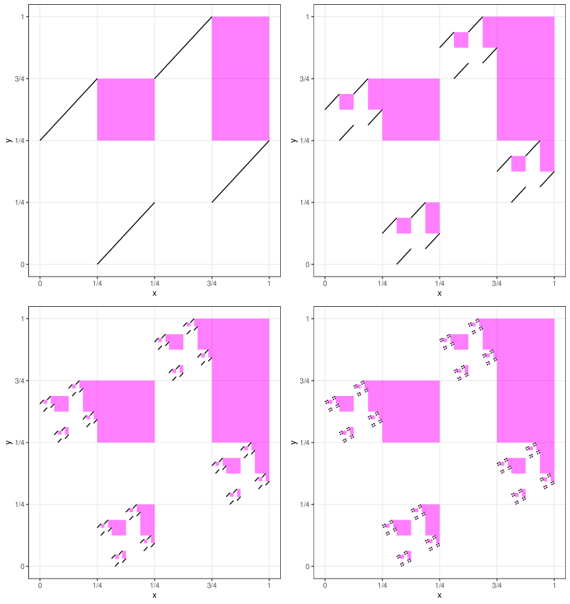
Figure 3: Supports of the copulas $V_{\pi}^{n}(M)$ (black line segments) and the corresponding sets $\Omega_{\sqrt{2}}^{V_{\pi}^{n}(M)}$ (magenta rectangles) for $n\in\{1,2,3,4\}$ and $\pi=(3,1,4,2)$ as considered in Example 4.4.

Acknowledgement
The second author gratefully acknowledge the support of the WISS 2025 project ‘IDA-lab Salzburg’ (20204-WISS/225/197-2019 and 20102-F1901166-KZP).

References

- [1] M. Coblenz, O. Grothe, M. Schreyer, W. Trutschnig: On the Length of Copula Level Curves, Journal of Multivariate Analysis 167, 347-365 (2018).
- [2] H. Daniels: Rank correlation and population models, Journal of the Royal Statistical Society: Series B (Methodological) 12, 171–191 (1950).
- [3] F. Durante, C. Sempi: Principles of copula theory, CRC/Chapman & Hall (2016).
- [4] J. Durbin, A. Stuart: Inversions and rank correlation coefficients, Journal of the Royal Statistical Society: Series B (Methodological) 13, 303-309 (1951).
- [5] L.C. Evans, R.F. Gariepy: Measure theory and fine Properties of Functions, Studies in Advanced Mathematics, CRC Press, Boca Raton, Florida (1992).
- [6] H. Federer: Geometric measure theory, Springer-Verlag (1969).
- [7] G.A. Fredricks, R.B. Nelsen, J.A. Rodríguez-Lallena: Copulas with fratal supports, Insur. Math. Econ. 37, 42-48 (2005).
- [8] O. Kallenberg: Foundations of modern probability, Probability and its Applications (New York), Springer-Verlag, New York, second edition (2002).
- [9] T. Kasper, S. Fuchs, W. Trutschnig: On weak conditional convergence of bivariate Archimedean and Extreme Value copulas, and consequences to nonparametric estimation, Bernoulli 27(4), 2217-2240 (2021).
- [10] A. Klenke: Wahrscheinlichkeitstheorie, Springer Lehrbuch Masterclass Series, Berlin Heidelberg (2008).
- [11] R.B. Nelsen: An introduction to copulas, Springer Science & Business Media, 2006.
- [12] M. Schreyer, R. Paulin, W. Trutschnig: On the exact region determined by Kendall’s tau and Spearman’s rho, Journal of the Royal Statistical Society: Series B (Statistical Methodology) 79(2), 613-633 (2017).
- [13] W. Trutschnig: On a strong metric on the space of copulas and its induced dependence measure, Journal of Mathematical Analysis and Applications 384, 690-705 (2011).
- [14] W. Trutschnig, J. Fernández Sánchez: Idempotent and multivariate copulas with fractal support, Journal of Statistical Planning and Inference 142, 3086-3096 (2012).