Closed-Loop Koopman Operator Approximation

Abstract

This paper proposes a method to identify a Koopman model of a feedback-controlled system given a known controller. The Koopman operator allows a nonlinear system to be rewritten as an infinite-dimensional linear system by viewing it in terms of an infinite set of lifting functions. A finite-dimensional approximation of the Koopman operator can be identified from data by choosing a finite subset of lifting functions and solving a regression problem in the lifted space. Existing methods are designed to identify open-loop systems. However, it is impractical or impossible to run experiments on some systems, such as unstable systems, in an open-loop fashion. The proposed method leverages the linearity of the Koopman operator, along with knowledge of the controller and the structure of the closed-loop system, to simultaneously identify the closed-loop and plant systems. The advantages of the proposed closed-loop Koopman operator approximation method are demonstrated experimentally using a rotary inverted pendulum system. An open-source software implementation of the proposed method is publicly available, along with the experimental dataset generated for this paper.

I Introduction

Using Koopman operator theory [1, 2, 3, 4], a finite-dimensional nonlinear system can be rewritten as an infinite-dimensional linear system. The Koopman operator itself serves to advance the infinite-dimensional system’s state in time, much like the dynamics matrix of a linear system. Practically working with an infinite-dimensional operator is intractable, so the Koopman operator is approximated as a finite-dimensional matrix, often using data-driven methods. While the Koopman operator was originally proposed almost one hundred years ago, recent theoretical results [2, 3, 4] paired with modern computational resources have led to it becoming a popular tool for identifying dynamical systems from data.

In a typical Koopman operator approximation workflow, a set of lifting functions is first chosen. In some situations, these lifting functions are inspired by the dynamics of the system [5, 6], while in others, they are taken from a standard set of basis functions, like polynomials, sinusoids, or radial basis functions [7, 8]. Lifting functions can also be chosen to approximate a given kernel [9, 10, 11]. Time delays are often incorporated into the lifted state as well [12, 7, 13]. Once the chosen lifting functions are applied to the data, linear regression is used to approximate the Koopman matrix, often with some form of regularization [7].

One of the key properties of the Koopman operator is its linearity, which makes it possible to leverage existing linear systems theory when identifying or analyzing Koopman systems. The linear Koopman representation of the nonlinear system also allows linear control design methods to be leveraged [12, 14, 5, 6, 7, 15]. Koopman operator approximation methods are also closely related to classical system identification methods [12, 16], most notably subspace identification methods [17, §3]. This similarity means that well-established system identification techniques can often be adapted to enrich the Koopman workflow.

An area of particular interest is the identification of closed-loop (CL) systems [18, 19, 20, 21]. It is often unsafe or impractical to run an experiment on a plant without a feedback control system [21, §1.1, §17.3]. In some cases, the control loop is simply ignored and the controller’s outputs are treated as exogenous input signals to the plant. However, this simplification, known as the direct approach to closed-loop system identification [21, §13.5], is problematic in some situations. The feedback loop introduces correlations between the plant’s output and its input, leading to biased estimates of the plant’s dynamics [18, 19], [22, §11.1]. In cases where this bias is small, the direct approach may yield acceptable results. In cases where the bias is not small, more sophisticated closed-loop system identification methods must be employed. The indirect approach to closed-loop system identification [21, §13.5], which uses the reference signal as the exogenous input, identifies the closed-loop system as a whole. The indirect approach then uses knowledge of the controller to extract a model of the plant system for use on its own [18, 19], [22, §11.1]. While closed-loop system identification can lead to more complex plant models, in many situations it is the appropriate tool to use to avoid biased estimates of model parameters.

Closed-loop identification is particularly practical when identifying unstable plants. Evaluating the performance of an unstable model is challenging, as prediction errors may diverge even if the identified model is accurate. This is particularly problematic in the Koopman framework, where lifting functions are unknown, and are often chosen based on the prediction error they achieve. By first identifying a model of the closed-loop system, which is assumed to be asymptotically stable, the closed-loop prediction error can be used as a more informative goodness-of-fit metric [18, §4.1]. Closed-loop identification methods also allow the closed-loop system’s model parameters to be regularized, when regularizing the unstable plant’s parameters may incorrectly lead to a stable model.

The key contribution of this paper is a means to identify a Koopman representation of a system using closed-loop data. The proposed method, summarized in Figure 1, is a variation of the indirect approach to system identification, wherein Koopman models of the closed-loop system and the plant system are simultaneously identified given knowledge of the controller. The significance of this work is that a system that cannot be operated in open-loop without a feedback controller can now be identified using Koopman operator theory. Even in situations where open-loop or closed-loop methods would identify the same model, it is shown that the closed-loop system is more convenient to work with, as it naturally provides a bounded prediction error and allows the closed-loop Koopman matrix to be included in a regularizer or additional constraint, such as an asymptotic stability constraint [23]. The advantages of the proposed method are demonstrated on a rotary inverted pendulum system which, due to its instability, would be difficult to identify in an open-loop setting.

Figure 1: Overview of the proposed closed-loop Koopman operator identification method. To simplify the presentation, no feedforward signal is used. (a) First, the controller reference, controller state, and plant state are recorded during a series of experiments. The controller state space matrices are known, and $\mbf{C}^{\mathrm{p}}$ and $\mbf{D}^{\mathrm{p}}$ are fixed. If the controller state is not directly available, it can be computed from its input and output. Only the Koopman matrix of the plant $\mbf{U}^{\mathrm{p}}$ is unknown. (b) The plant state is lifted and augmented with the controller state and reference. (c) The Koopman matrices of the closed-loop (CL) system and the plant system are approximated simultaneously by incorporating the known structure of the closed-loop system as a constraint on the Extended DMD (EDMD) problem.

The remainder of this paper is as follows. Section II outlines the necessary background information on the Koopman operator and its associated approximation techniques. Section III derives the proposed closed-loop Koopman operator approximation method. Section IV analyzes the experimental results of the closed-loop Koopman operator approximation method. Finally, Section V presents the paper’s conclusions and discusses avenues for future research.

II Background

II-A Koopman operator theory

Consider the nonlinear difference equation

$$\mbf{x}_{k+1}=\mbf{f}(\mbf{x}_{k}),$$ (1)

where ${\mbf{x}_{k}\in\mathcal{M}}$ evolves on a manifold ${\mathcal{M}\subseteq\mathbb{R}^{m\times 1}}$. Also consider an infinite number of scalar-valued lifting functions, ${\psi:\mathcal{M}\to\mathbb{R}}$, which span an infinite-dimensional Hilbert space $\mathcal{H}$. The Koopman operator, ${\mathcal{U}:\mathcal{H}\to\mathcal{H}}$, is a linear operator that composes all lifting functions ${\psi\in\mathcal{H}}$ with $\mbf{f}(\cdot)$, thereby advancing them in time by one step. That is [24, §3.2],

$$(\mathcal{U}\psi)(\cdot)=(\psi\circ\mbf{f})(\cdot).$$ (2)

Evaluating (2) at $\mbf{x}_{k}$ reveals that the dynamics of (1) can be rewritten linearly in terms of $\psi$ as

$$\psi(\mbf{x}_{k+1})=(\mathcal{U}\psi)(\mbf{x}_{k}).$$ (3)

A finite-dimensional approximation of (3) is

$$\bm{\psi}(\mbf{x}_{k+1})=\mbf{U}\bm{\psi}(\mbf{x}_{k})+\bm{\epsilon}_{k},$$ (4)

where ${\bm{\psi}:\mathcal{M}\to\mathbb{R}^{p\times 1}}$ is the vector-valued lifting function, ${\mbf{U}\in\mathbb{R}^{p\times p}}$ is the Koopman matrix, and $\bm{\epsilon}_{k}$ is the residual error.

II-B Koopman operator theory with inputs

The definition of the Koopman operator can be modified to accommodate nonlinear difference equations with exogenous inputs. Consider the difference equation

$$\mbf{x}_{k+1}=\mbf{f}(\mbf{x}_{k},\mbf{u}_{k}),$$ (5)

where the state is ${\mbf{x}_{k}\in\mathcal{M}\subseteq\mathbb{R}^{m\times 1}}$ and the input is ${\mbf{u}_{k}\in\mathcal{N}\subseteq\mathbb{R}^{n\times 1}}$. The lifting functions are now ${\psi:\mathcal{M}\times\mathcal{N}\to\mathbb{R}}$ and the Koopman operator ${\mathcal{U}:\mathcal{H}\to\mathcal{H}}$ now satisfies

$$(\mathcal{U}\psi)(\mbf{x}_{k},\mbf{u}_{k})=\psi(\mbf{f}(\mbf{x}_{k},\mbf{u}_{k}),\star),$$ (6)

where ${\star=\mbf{u}_{k}}$ if the input has state-dependent dynamics, or ${\star=\mbf{0}}$ if the input has no dynamics [24, §6.5]. Let the vector-valued lifting function ${\bm{\psi}:\mathcal{M}\times\mathcal{N}\to\mathbb{R}^{p\times 1}}$ be partitioned as

$$\bm{\psi}(\mbf{x}_{k},\mbf{u}_{k})=\begin{bmatrix}\bm{\vartheta}(\mbf{x}_{k})\\ \bm{\upsilon}(\mbf{x}_{k},\mbf{u}_{k})\end{bmatrix},$$ (7)

where the state-dependent lifting functions are ${\bm{\vartheta}:\mathcal{M}\to\mathbb{R}^{p_{\vartheta}\times 1}}$, the input-dependent lifting functions are ${\bm{\upsilon}:\mathcal{M}\times\mathcal{N}\to\mathbb{R}^{p_{\upsilon}\times 1}}$, and the lifting function dimensions satisfy ${p_{\vartheta}+p_{\upsilon}=p}$. With an exogenous input, substituting the state and input into (6) results in [24, §6.5.1]

$$\bm{\vartheta}(\mbf{x}_{k+1})\\ =\mbf{U}\bm{\psi}(\mbf{x}_{k},\mbf{u}_{k})+\bm{\epsilon}_{k},$$ (8)

where ${\mbf{U}=\begin{bmatrix}\mbf{A}&\mbf{B}\end{bmatrix}}$. Expanding (8) yields the familiar linear state-space form,

$$\bm{\vartheta}(\mbf{x}_{k+1})=\mbf{A}\bm{\vartheta}(\mbf{x}_{k})+\mbf{B}\bm{\upsilon}(\mbf{x}_{k},\mbf{u}_{k})+\bm{\epsilon}_{k}.$$ (9)

When designing lifting functions, the first $m$ lifted states are often chosen to be the state of the original difference equation, $\mbf{x}_{k}$. Specifically, [24, §3.3.1]

$$\bm{\vartheta}(\mbf{x}_{k})=\begin{bmatrix}\mbf{x}_{k}\\ \vartheta_{m}(\mbf{x}_{k})\\ \vartheta_{m+1}(\mbf{x}_{k})\\ \vdots\\ \vartheta_{p_{\vartheta}-1}(\mbf{x}_{k})\end{bmatrix}.$$ (10)

This choice of lifting functions makes it easier to recover the original state from the lifted state. Another common design decision is to leave the input unlifted when identifying a Koopman model for control. That is [12],

$$\bm{\upsilon}(\mbf{x}_{k},\mbf{u}_{k})=\mbf{u}_{k}.$$ (11)

However, recent work has also shown that bilinear input-dependent lifting functions are a better alternative for control affine systems [25].

An output equation,

$$\bm{\zeta}_{k}=\mbf{C}\bm{\vartheta}_{k}+\mbf{D}\bm{\upsilon}_{k},$$ (12)

where $\bm{\zeta}_{k}\in\mathbb{R}^{p_{\zeta}\times 1}$, can also be considered to incorporate the Koopman operator into a true linear system with input, output, and state. While $\mbf{D}=\mbf{0}$ in all cases, $\mbf{C}$ can be chosen to recover the original states, or any other desired output. If the original state is not directly included in the lifted state, $\mbf{C}$ can instead be determined using least-squares [12, §3.2.1]. The Koopman system is therefore

$$\bm{\mathcal{G}}\stackrel{{\scriptstyle\min}}{{\sim}}\left[\begin{array}[]{c|c}\mbf{A}&\mbf{B}\\ \hline\cr\mbf{C}&\mbf{D}\end{array}\right],$$ (13)

where $\stackrel{{\scriptstyle\min}}{{\sim}}$ denotes a minimal state space realization [26, §3.2.1].

II-C Approximation of the Koopman operator from data

To approximate the Koopman matrix from a dataset ${\mathcal{D}={\{\mbf{x}_{k},\mbf{u}_{k}\}}_{k=0}^{q}}$, consider the lifted snapshot matrices

$$\bm{\Psi} =\begin{bmatrix}\bm{\psi}_{0}&\bm{\psi}_{1}&\cdots&\bm{\psi}_{q-1}\end{bmatrix}\in\mathbb{R}^{p\times q},$$ (14)

$$\bm{\Theta}_{+} =\begin{bmatrix}\bm{\vartheta}_{1}&\bm{\vartheta}_{2}&\cdots&\bm{\vartheta}_{q}\end{bmatrix}\in\mathbb{R}^{p_{\vartheta}\times q},$$ (15)

where ${\bm{\psi}_{k}=\bm{\psi}(\mbf{x}_{k},\mbf{u}_{k})}$ and ${\bm{\vartheta}_{k}=\bm{\vartheta}(\mbf{x}_{k})}$. The Koopman matrix that minimizes

$$J(\mbf{U})=\frac{1}{q}\|\bm{\Theta}_{+}-\mbf{U}\bm{\Psi}\|_{\mathsf{F}}^{2}$$ (16)

is [24, §1.2.1]

$$\mbf{U}=\bm{\Theta}_{+}\bm{\Psi}^{\dagger},$$ (17)

where ${(\cdot)}^{\dagger}$ denotes the Moore-Penrose pseudoinverse.

When the dataset contains many snapshots, the pseudoinverse required in (17) is numerically ill-conditioned. Extended Dynamic Mode Decomposition (EDMD) [27] can alleviate this problem when dataset contains many fewer states than snapshots (i.e., when $p\ll q$) [24, §10.3]. The EDMD approximation of the Koopman matrix is

$$\mbf{U}=\bm{\Theta}_{+}\left(\bm{\Psi}^{\mathsf{T}}\bm{\Psi}^{{\mathsf{T}}^{\dagger}}\right)\bm{\Psi}^{\dagger}=\left(\bm{\Theta}_{+}\bm{\Psi}^{\mathsf{T}}\right){\left(\bm{\Psi}\bm{\Psi}^{\mathsf{T}}\right)}^{\dagger}=\mbf{G}\mbf{H}^{\dagger},$$ (18)

where

$$\mbf{G}=\frac{1}{q}\bm{\Theta}_{+}\bm{\Psi}^{\mathsf{T}}\in\mathbb{R}^{p_{\vartheta}\times p},\quad\mbf{H}=\frac{1}{q}\bm{\Psi}\bm{\Psi}^{\mathsf{T}}\in\mathbb{R}^{p\times p}.$$ (19)

Often, Tikhonov regularization is also included to improve the numerical conditioning of $\mbf{U}$ by penalizing its squared Frobenius norm [28]. The cost function then becomes

$$J(\mbf{U})=\frac{1}{q}\|\bm{\Theta}_{+}-\mbf{U}\bm{\Psi}\|_{\mathsf{F}}^{2}+\frac{\alpha}{q}\|\mbf{U}\|_{\mathsf{F}}^{2},$$ (20)

where $\alpha$ is the regularization coefficient. The incorporation of Tikhonov regularization into EDMD is discussed in Section III.

III Closed-loop Koopman operator approximation

In this section, the proposed closed-loop Koopman operator approximation method is outlined in detail. First, the Koopman representation of the closed-loop system is derived in terms of the known state-space matrices of the controller and the unknown Koopman matrix of the plant. Then, a method for simultaneously identifying the closed-loop system and plant system is described.

III-A Formulation of the closed-loop Koopman system

Consider the Koopman system modelling the plant,

$$\bm{\vartheta}_{k+1}^{\mathrm{p}} =\mbf{A}^{\!\mathrm{p}}\bm{\vartheta}_{k}^{\mathrm{p}}+\mbf{B}^{\mathrm{p}}\bm{\upsilon}_{k}^{\mathrm{p}},$$ (21)

$$\bm{\zeta}_{k}^{\mathrm{p}} =\mbf{C}^{\mathrm{p}}\bm{\vartheta}_{k}^{\mathrm{p}}+\mbf{D}^{\mathrm{p}}\bm{\upsilon}_{k}^{\mathrm{p}},$$ (22)

along with the linear system modelling the known controller,

$$\mbf{x}_{k+1}^{\mathrm{c}} =\mbf{A}^{\!\mathrm{c}}\mbf{x}_{k}^{\mathrm{c}}+\mbf{B}^{\mathrm{c}}\mbf{u}_{k}^{\mathrm{c}},$$ (23)

$$\mbf{y}_{k}^{\mathrm{c}} =\mbf{C}^{\mathrm{c}}\mbf{x}_{k}^{\mathrm{c}}+\mbf{D}^{\mathrm{c}}\mbf{u}_{k}^{\mathrm{c}}.$$ (24)

Let

$$\bm{\upsilon}_{k}^{\mathrm{p}}=\mbf{y}_{k}^{\mathrm{c}}+\mbf{f}_{k},$$ (25)

which yields the series interconnection of the controller and the plant with a feedforward signal $\mbf{f}_{k}$. This feedforward signal is entirely exogenous, and could be generated by a nonlinear inverse model of the plant. The new Koopman system’s input includes the controller input and feedforward input, resulting in

$$\bm{\upsilon}_{k}^{\mathrm{s}}=\begin{bmatrix}\mbf{u}_{k}^{\mathrm{c}}\\ \mbf{f}_{k}\end{bmatrix},$$ (26)

while its output is simply the plant output, ${\bm{\zeta}_{k}=\bm{\zeta}_{k}^{\mathrm{p}}}$. The new system’s state includes the controller state and plant state, resulting in

$$\bm{\vartheta}_{k}=\begin{bmatrix}\mbf{x}_{k}^{\mathrm{c}}\\ \bm{\vartheta}_{k}^{\mathrm{p}}\end{bmatrix}.$$ (27)

The cascaded plant and controller systems are depicted in Figure 2.

Figure 2: Series interconnection of the controller and plant.

The state space representation of the plant becomes

$$\bm{\vartheta}_{k+1}^{\mathrm{p}} =\mbf{A}^{\!\mathrm{p}}\bm{\vartheta}_{k}^{\mathrm{p}}+\mbf{B}^{\mathrm{p}}\left(\mbf{C}^{\mathrm{c}}\mbf{x}_{k}^{\mathrm{c}}+\mbf{D}^{\mathrm{c}}\mbf{u}_{k}^{\mathrm{c}}+\mbf{f}_{k}\right)$$ (28)

$$=\begin{bmatrix}\mbf{B}^{\mathrm{p}}\mbf{C}^{\mathrm{c}}&\mbf{A}^{\!\mathrm{p}}\end{bmatrix}\begin{bmatrix}\mbf{x}_{k}^{\mathrm{c}}\\ \bm{\vartheta}_{k}^{\mathrm{p}}\end{bmatrix}+\begin{bmatrix}\mbf{B}^{\mathrm{p}}\mbf{D}^{\mathrm{c}}&\mbf{B}^{\mathrm{p}}\end{bmatrix}\begin{bmatrix}\mbf{u}_{k}^{\mathrm{c}}\\ \mbf{f}_{k}\end{bmatrix},$$ (29)

$$\bm{\zeta}_{k}^{\mathrm{p}} =\mbf{C}^{\mathrm{p}}\bm{\vartheta}_{k}^{\mathrm{p}}+\mbf{D}^{\mathrm{p}}\left(\mbf{C}^{\mathrm{c}}\mbf{x}_{k}^{\mathrm{c}}+\mbf{D}^{\mathrm{c}}\mbf{u}_{k}^{\mathrm{c}}+\mbf{f}_{k}\right)$$ (30)

$$=\begin{bmatrix}\mbf{D}^{\mathrm{p}}\mbf{C}^{\mathrm{c}}&\mbf{C}^{\mathrm{p}}\end{bmatrix}\begin{bmatrix}\mbf{x}_{k}^{\mathrm{c}}\\ \bm{\vartheta}_{k}^{\mathrm{p}}\end{bmatrix}+\begin{bmatrix}\mbf{D}^{\mathrm{p}}\mbf{D}^{\mathrm{c}}&\mbf{D}^{\mathrm{p}}\end{bmatrix}\begin{bmatrix}\mbf{u}_{k}^{\mathrm{c}}\\ \mbf{f}_{k}\end{bmatrix}.$$ (31)

The state space representation of the series-interconnected system is therefore

$$\begin{bmatrix}\mbf{x}_{k+1}^{\mathrm{c}}\\ \bm{\vartheta}_{k+1}^{\mathrm{p}}\end{bmatrix} =\begin{bmatrix}\mbf{A}^{\!\mathrm{c}}&\mbf{0}\\ \mbf{B}^{\mathrm{p}}\mbf{C}^{\mathrm{c}}&\mbf{A}^{\!\mathrm{p}}\end{bmatrix}\begin{bmatrix}\mbf{x}_{k}^{\mathrm{c}}\\ \bm{\vartheta}_{k}^{\mathrm{p}}\end{bmatrix}+\begin{bmatrix}\mbf{B}^{\mathrm{c}}&\mbf{0}\\ \mbf{B}^{\mathrm{p}}\mbf{D}^{\mathrm{c}}&\mbf{B}^{\mathrm{p}}\end{bmatrix}\begin{bmatrix}\mbf{u}_{k}^{\mathrm{c}}\\ \mbf{f}_{k}\end{bmatrix},$$ (32)

$$\bm{\zeta}_{k}^{\mathrm{p}} =\begin{bmatrix}\mbf{D}^{\mathrm{p}}\mbf{C}^{\mathrm{c}}&\mbf{C}^{\mathrm{p}}\end{bmatrix}\begin{bmatrix}\mbf{x}_{k}^{\mathrm{c}}\\ \bm{\vartheta}_{k}^{\mathrm{p}}\end{bmatrix}+\begin{bmatrix}\mbf{D}^{\mathrm{p}}\mbf{D}^{\mathrm{c}}&\mbf{D}^{\mathrm{p}}\end{bmatrix}\begin{bmatrix}\mbf{u}_{k}^{\mathrm{c}}\\ \mbf{f}_{k}\end{bmatrix},$$ (33)

or equivalently,

$$\bm{\vartheta}_{k+1} =\begin{bmatrix}\mbf{A}^{\!\mathrm{c}}&\mbf{0}\\ \mbf{B}^{\mathrm{p}}\mbf{C}^{\mathrm{c}}&\mbf{A}^{\!\mathrm{p}}\end{bmatrix}\bm{\vartheta}_{k}+\begin{bmatrix}\mbf{B}^{\mathrm{c}}&\mbf{0}\\ \mbf{B}^{\mathrm{p}}\mbf{D}^{\mathrm{c}}&\mbf{B}^{\mathrm{p}}\end{bmatrix}\bm{\upsilon}_{k}^{\mathrm{s}},$$ (34)

$$\bm{\zeta}_{k} =\begin{bmatrix}\mbf{D}^{\mathrm{p}}\mbf{C}^{\mathrm{c}}&\mbf{C}^{\mathrm{p}}\end{bmatrix}\bm{\vartheta}_{k}+\begin{bmatrix}\mbf{D}^{\mathrm{p}}\mbf{D}^{\mathrm{c}}&\mbf{D}^{\mathrm{p}}\end{bmatrix}\bm{\upsilon}_{k}^{\mathrm{s}}.$$ (35)

Next, consider the negative feedback interconnection,

$$\mbf{u}_{k}^{\mathrm{c}}=\mbf{r}_{k}-\bm{\zeta}_{k},$$ (36)

where $\mbf{r}_{k}$ is an exogenous reference signal. The input of this new feedback-interconnected system is defined to be

$$\bm{\upsilon}_{k}=\begin{bmatrix}\mbf{r}_{k}\\ \mbf{f}_{k}\end{bmatrix},$$ (37)

as depicted in Figure 3. Substituting (36) into (26) yields

$$\bm{\upsilon}_{k}^{\mathrm{s}} =\begin{bmatrix}\mbf{r}_{k}-\bm{\zeta}_{k}\\ \mbf{f}_{k}\end{bmatrix}$$ (38)

$$=\bm{\upsilon}_{k}-\begin{bmatrix}\bm{\zeta}_{k}\\ \mbf{0}\end{bmatrix}.$$ (39)

Figure 3: Feedback interconnection of the controller and plant.

Substituting (39) into (35) results in a new output equation,

$$\bm{\zeta}_{k}={\left(\mbf{1}+\mbf{D}^{\mathrm{p}}\mbf{D}^{\mathrm{c}}\right)}^{-1}\begin{bmatrix}\mbf{D}^{\mathrm{p}}\mbf{C}^{\mathrm{c}}&\mbf{C}^{\mathrm{p}}\end{bmatrix}\bm{\vartheta}_{k}\\ +{\left(\mbf{1}+\mbf{D}^{\mathrm{p}}\mbf{D}^{\mathrm{c}}\right)}^{-1}\begin{bmatrix}\mbf{D}^{\mathrm{p}}\mbf{D}^{\mathrm{c}}&\mbf{D}^{\mathrm{p}}\end{bmatrix}\bm{\upsilon}_{k},$$ (40)

where the feedback interconnection is well-posed if and only if ${\mbf{1}+\mbf{D}^{\mathrm{p}}\mbf{D}^{\mathrm{c}}}$ is invertible [29, §4.9.1]. Let ${\mbf{Q}=\mbf{1}+\mbf{D}^{\mathrm{p}}\mbf{D}^{\mathrm{c}}}$. Substituting (40) into (39) yields

$$\bm{\upsilon}_{k}^{\mathrm{s}}=\begin{bmatrix}-{\mbf{Q}}^{-1}\mbf{D}^{\mathrm{p}}\mbf{C}^{\mathrm{c}}&-{\mbf{Q}}^{-1}\mbf{C}^{\mathrm{p}}\\ \mbf{0}&\mbf{0}\end{bmatrix}\bm{\vartheta}_{k}\\ +\begin{bmatrix}\mbf{1}-{\mbf{Q}}^{-1}\mbf{D}^{\mathrm{p}}\mbf{D}^{\mathrm{c}}&-{\mbf{Q}}^{-1}\mbf{D}^{\mathrm{p}}\\ \mbf{0}&\mbf{1}\end{bmatrix}\bm{\upsilon}_{k}.$$ (41)

Substituting (41) back into (34) and rearranging results in a new state equation,

$$\bm{\vartheta}_{k+1}=\begin{bmatrix}\mbf{A}^{\!\mathrm{c}}-\mbf{B}^{\mathrm{c}}{\mbf{Q}}^{-1}\mbf{D}^{\mathrm{p}}\mbf{C}^{\mathrm{c}}&-\mbf{B}^{\mathrm{c}}{\mbf{Q}}^{-1}\mbf{C}^{\mathrm{p}}\\ \mbf{B}^{\mathrm{p}}\mbf{C}^{\mathrm{c}}-\mbf{B}^{\mathrm{p}}\mbf{D}^{\mathrm{c}}{\mbf{Q}}^{-1}\mbf{D}^{\mathrm{p}}\mbf{C}^{\mathrm{c}}&\mbf{A}^{\!\mathrm{p}}-\mbf{B}^{\mathrm{p}}\mbf{D}^{\mathrm{c}}{\mbf{Q}}^{-1}\mbf{C}^{\mathrm{p}}\\ \end{bmatrix}\bm{\vartheta}_{k}\\ +\begin{bmatrix}\mbf{B}^{\mathrm{c}}-\mbf{B}^{\mathrm{c}}{\mbf{Q}}^{-1}\mbf{D}^{\mathrm{p}}\mbf{D}^{\mathrm{c}}&-\mbf{B}^{\mathrm{c}}{\mbf{Q}}^{-1}\mbf{D}^{\mathrm{p}}\\ \mbf{B}^{\mathrm{p}}\mbf{D}^{\mathrm{c}}-\mbf{B}^{\mathrm{p}}\mbf{D}^{\mathrm{c}}{\mbf{Q}}^{-1}\mbf{D}^{\mathrm{p}}\mbf{D}^{\mathrm{c}}&\mbf{B}^{\mathrm{p}}-\mbf{B}^{\mathrm{p}}\mbf{D}^{\mathrm{c}}{\mbf{Q}}^{-1}\mbf{D}^{\mathrm{p}}\end{bmatrix}\bm{\upsilon}_{k},$$ (42)

and the output equation being

$$\bm{\zeta}_{k}=\begin{bmatrix}{\mbf{Q}}^{-1}\mbf{D}^{\mathrm{p}}\mbf{C}^{\mathrm{c}}&{\mbf{Q}}^{-1}\mbf{C}^{\mathrm{p}}\end{bmatrix}\bm{\vartheta}_{k}+\begin{bmatrix}{\mbf{Q}}^{-1}\mbf{D}^{\mathrm{p}}\mbf{D}^{\mathrm{c}}&{\mbf{Q}}^{-1}\mbf{D}^{\mathrm{p}}\end{bmatrix}\bm{\upsilon}_{k}.$$ (43)

In the Koopman system, only $\mbf{A}^{\!\mathrm{p}}$ and $\mbf{B}^{\mathrm{p}}$ are determined from experimental data. The remaining state-space matrices are chosen to be

$$\mbf{C}^{\mathrm{p}} =\begin{bmatrix}\mbf{1}_{m\times m}&\mbf{0}_{m\times(p_{\vartheta}-m)}\end{bmatrix},$$ (44)

$$\mbf{D}^{\mathrm{p}} =\mbf{0},$$ (45)

such that $\mbf{C}^{\mathrm{p}}$ recovers the controlled states of the nonlinear system being modelled, which are the first $m$ states in $\bm{\vartheta}_{k}^{\mathrm{p}}$. Substituting in (45) implies that ${\mbf{Q}=\mbf{1}}$. Thus, the simplified state-space representation of the closed-loop system is

$$\bm{\vartheta}_{k+1} =\underbrace{\begin{bmatrix}\mbf{A}^{\!\mathrm{c}}&-\mbf{B}^{\mathrm{c}}\mbf{C}^{\mathrm{p}}\\ \mbf{B}^{\mathrm{p}}\mbf{C}^{\mathrm{c}}&\mbf{A}^{\!\mathrm{p}}-\mbf{B}^{\mathrm{p}}\mbf{D}^{\mathrm{c}}\mbf{C}^{\mathrm{p}}\\ \end{bmatrix}}_{\mbf{A}^{\!\mathrm{f}}}\bm{\vartheta}_{k}+\underbrace{\begin{bmatrix}\mbf{B}^{\mathrm{c}}&\mbf{0}\\ \mbf{B}^{\mathrm{p}}\mbf{D}^{\mathrm{c}}&\mbf{B}^{\mathrm{p}}\end{bmatrix}}_{\mbf{B}^{\mathrm{f}}}\bm{\upsilon}_{k},$$ (46)

$$\bm{\zeta}_{k} =\underbrace{\begin{bmatrix}\mbf{0}&\mbf{C}^{\mathrm{p}}\end{bmatrix}}_{\mbf{C}^{\mathrm{f}}}\bm{\vartheta}_{k}+\underbrace{\mbf{0}}_{\mbf{D}^{\mathrm{f}}}\,\bm{\upsilon}_{k},$$ (47)

which is always a well-posed feedback interconnection, since ${\mbf{Q}=\mbf{1}+\mbf{D}^{\mathrm{p}}\mbf{D}^{\mathrm{c}}=\mbf{1}}$ is invertible.

III-B Identification of the closed-loop and plant systems

Consider the closed-loop lifted dataset ${\mathcal{D}={\left\{\bm{\vartheta}_{k},\bm{\upsilon}_{k}\right\}}_{k=0}^{q}}$, where the matrix approximation of the Koopman operator is

$$\mbf{U}^{\mathrm{f}} =\begin{bmatrix}\mbf{U}_{11}^{\mathrm{f}}&\mbf{U}_{12}^{\mathrm{f}}&\mbf{U}_{13}^{\mathrm{f}}&\mbf{U}_{14}^{\mathrm{f}}\\ \mbf{U}_{21}^{\mathrm{f}}&\mbf{U}_{22}^{\mathrm{f}}&\mbf{U}_{23}^{\mathrm{f}}&\mbf{U}_{24}^{\mathrm{f}}\end{bmatrix}.$$ (48)

$$=\begin{bmatrix}\mbf{A}^{\!\mathrm{c}}&-\mbf{B}^{\mathrm{c}}\mbf{C}^{\mathrm{p}}&\mbf{B}^{\mathrm{c}}&\mbf{0}\\ \mbf{B}^{\mathrm{p}}\mbf{C}^{\mathrm{c}}&\mbf{A}^{\!\mathrm{p}}-\mbf{B}^{\mathrm{p}}\mbf{D}^{\mathrm{c}}\mbf{C}^{\mathrm{p}}&\mbf{B}^{\mathrm{p}}\mbf{D}^{\mathrm{c}}&\mbf{B}^{\mathrm{p}}\end{bmatrix}$$ (49)

Comparing (48) and (49) reveals that the matrices, $\mbf{B}^{\mathrm{p}}$, $\mbf{U}_{21}^{\mathrm{f}}$, $\mbf{U}_{23}^{\mathrm{f}}$, and $\mbf{U}_{24}^{\mathrm{f}}$ are related via the expression

$$\mbf{B}^{\mathrm{p}}{\begin{bmatrix}\mbf{C}^{\mathrm{c}}&\mbf{D}^{\mathrm{c}}&\mbf{1}\vphantom{\mbf{U}_{24}^{\mathrm{f}}}\end{bmatrix}}=\begin{bmatrix}\mbf{U}_{21}^{\mathrm{f}}&\mbf{U}_{23}^{\mathrm{f}}&\mbf{U}_{24}^{\mathrm{f}}\end{bmatrix}.$$ (50)

Thus, one way to compute $\mbf{U}^{\mathrm{p}}=\begin{bmatrix}\mbf{A}^{\!\mathrm{p}}&\mbf{B}^{\mathrm{p}}\end{bmatrix}$ is to first compute $\mbf{U}^{\mathrm{f}}$ using EDMD and then recover the plant’s state space matrices using

$$\mbf{B}^{\mathrm{p}} =\begin{bmatrix}\mbf{U}_{21}^{\mathrm{f}}&\mbf{U}_{23}^{\mathrm{f}}&\mbf{U}_{24}^{\mathrm{f}}\end{bmatrix}{\begin{bmatrix}\mbf{C}^{\mathrm{c}}&\mbf{D}^{\mathrm{c}}&\mbf{1}\vphantom{\mbf{U}_{24}^{\mathrm{f}}}\end{bmatrix}}^{\dagger},$$ (51)

$$\mbf{A}^{\!\mathrm{p}} =\mbf{U}_{22}^{\mathrm{f}}+\mbf{B}^{\mathrm{p}}\mbf{D}^{\mathrm{c}}\mbf{C}^{\mathrm{p}}.$$ (52)

While this approach is simple, it is not guaranteed to preserve the required relationships between $\mbf{U}^{\mathrm{f}}$, $\mbf{A}^{\!\mathrm{p}}$, and $\mbf{B}^{\mathrm{c}}$ found in (48) and (49). As a result, identifying the closed-loop system, extracting the plant model with (51) and (52), and then closing the loop again with the same controller using (49) can result in an entirely different closed-loop system. This pitfall is explored further in the Appendix.

To preserve the structure of the closed-loop system, (50) and (52) can be treated as constraints when identifying the Koopman matrix of the closed-loop system. Including Tikhonov regularization, the resulting EDMD optimization problem is

$$\min\; J(\mbf{U}^{\mathrm{f}},\mbf{U}^{\mathrm{p}};\alpha)=\frac{1}{q}\big{\|}\bm{\Theta}_{+}-\mbf{U}^{\mathrm{f}}\bm{\Psi}\big{\|}_{\mathsf{F}}^{2}+\frac{\alpha}{q}\big{\|}\mbf{U}^{\mathrm{f}}\big{\|}_{\mathsf{F}}^{2}$$ (53)

$$\mathrm{s.t.}\; \begin{bmatrix}\mbf{U}_{21}^{\mathrm{f}}&\mbf{U}_{23}^{\mathrm{f}}&\mbf{U}_{24}^{\mathrm{f}}\end{bmatrix}=\mbf{B}^{\mathrm{p}}\begin{bmatrix}\mbf{C}^{\mathrm{c}}&\mbf{D}^{\mathrm{c}}&\mbf{1}\end{bmatrix},$$ (54)

$$\mbf{U}_{22}^{\mathrm{f}}=\mbf{A}^{\!\mathrm{p}}-\mbf{B}^{\mathrm{p}}\mbf{D}^{\mathrm{c}}\mbf{C}^{\mathrm{p}}.$$ (55)

To efficiently solve the optimization problem posed in (53)–(55), its cost function is reformulated as a semidefinite program in a manner similar to [30, 23]. The cost function in (53) can be rewritten as

$$J(\mbf{U}^{\mathrm{f}};\alpha)=\frac{1}{q}{\mathrm{tr}}{\left(\bm{\Theta}_{+}\bm{\Theta}_{+}^{\mathsf{T}}-{\mathrm{He}\!\left\{\mbf{U}^{\mathrm{f}}\bm{\Psi}\bm{\Theta}_{+}^{\mathsf{T}}\right\}}+\mbf{U}^{\mathrm{f}}\bm{\Psi}\bm{\Psi}^{\mathsf{T}}\mbf{U}^{\mathrm{f}^{\mathsf{T}}}\right)}\\ +\frac{\alpha}{q}{\mathrm{tr}}{\left(\mbf{U}^{\mathrm{f}}\mbf{U}^{\mathrm{f}^{\mathsf{T}}}\right)},$$ (56)

where ${\mathrm{He}\!\left\{\cdot\right\}}=(\cdot)+{(\cdot)}^{\mathsf{T}}$. Substituting in (19) yields

$$J(\mbf{U}^{\mathrm{f}};\alpha)={\mathrm{tr}}{\left(\mbf{F}-{\mathrm{He}\!\left\{\mbf{U}^{\mathrm{f}}\mbf{G}^{\mathsf{T}}\right\}}+\mbf{U}^{\mathrm{f}}\mbf{H}_{\alpha}\mbf{U}^{\mathrm{f}^{\mathsf{T}}}\right)},$$ (57)

where $\mbf{F}=\frac{1}{q}\bm{\Theta}_{+}\bm{\Theta}_{+}^{\mathsf{T}}$ and $\mbf{H}_{\alpha}=\mbf{H}+\frac{\alpha}{q}\mbf{1}$. Introducing a slack variable [31, §2.15.1] results in the equivalent unconstrained optimization problem,

$$\min\; J(\mbf{U}^{\mathrm{f}},\mbf{W};\alpha)={\mathrm{tr}}{\left(\mbf{W}\right)}$$ (58)

$$\mathrm{s.t.}\; \mbf{W}>0,$$ (59)

$$\mbf{F}-{\mathrm{He}\!\left\{\mbf{U}^{\mathrm{f}}\mbf{G}^{\mathsf{T}}\right\}}+\mbf{U}^{\mathrm{f}}\mbf{H}_{\alpha}\mbf{U}^{\mathrm{f}^{\mathsf{T}}}<\mbf{W}.$$ (60)

Next, the Schur complement is used to break up the quadratic term in (60) [31, §2.3.1]. Equation (19) shows that ${\mbf{H}=\mbf{H}^{\mathsf{T}}>0}$ if the columns of $\bm{\Psi}$ are linearly independent. Assuming that $\mbf{H}_{\alpha}$ is positive definite, consider its Cholesky factorization, $\mbf{H}_{\alpha}=\mbf{R}_{\alpha}\mbf{R}_{\alpha}^{\mathsf{T}}$. Substituting in the Cholesky factorization and applying the Schur complement yields the semidefinite program,

$$\min\; J(\mbf{U}^{\mathrm{f}},\mbf{W};\alpha)={\mathrm{tr}}\left(\mbf{W}\right)$$ (61)

$$\mathrm{s.t.}\; \mbf{W}>0,$$ (62)

$$\begin{bmatrix}-\mbf{W}+\mbf{F}-{\mathrm{He}\!\left\{\mbf{U}^{\mathrm{f}}\mbf{G}^{\mathsf{T}}\right\}}&\mbf{U}^{\mathrm{f}}\mbf{R}_{\alpha}\\ \mbf{R}_{\alpha}^{\mathsf{T}}\mbf{U}^{\mathrm{f}^{\mathsf{T}}}&-\mbf{1}\end{bmatrix}<0.$$ (63)

Including the structural constraints on the closed-loop system from (50) and (52) results in

$$\min\; J(\mbf{U}^{\mathrm{f}},\mbf{U}^{\mathrm{p}},\mbf{W};\alpha)={\mathrm{tr}}\left(\mbf{W}\right)$$ (64)

$$\mathrm{s.t.}\; \mbf{W}>0,$$ (65)

$$\begin{bmatrix}-\mbf{W}+\mbf{F}-{\mathrm{He}\!\left\{\mbf{U}^{\mathrm{f}}\mbf{G}^{\mathsf{T}}\right\}}&\mbf{U}^{\mathrm{f}}\mbf{R}_{\alpha}\\ \mbf{R}_{\alpha}^{\mathsf{T}}\mbf{U}^{\mathrm{f}^{\mathsf{T}}}&-\mbf{1}\end{bmatrix}<0,$$ (66)

$$\begin{bmatrix}\mbf{U}_{21}^{\mathrm{f}}&\mbf{U}_{23}^{\mathrm{f}}&\mbf{U}_{24}^{\mathrm{f}}\end{bmatrix}=\mbf{B}^{\mathrm{p}}\begin{bmatrix}\mbf{C}^{\mathrm{c}}&\mbf{D}^{\mathrm{c}}&\mbf{1}\end{bmatrix},$$ (67)

$$\mbf{U}_{22}^{\mathrm{f}}=\mbf{A}^{\!\mathrm{p}}-\mbf{B}^{\mathrm{p}}\mbf{D}^{\mathrm{c}}\mbf{C}^{\mathrm{p}},$$ (68)

which provides a means to simultaneously identify a Koopman model of the closed-loop system and the plant system. While this method applies Tikhonov regularization to the closed-loop system’s Koopman matrix, any regularizer or constraint, such as those in [30, 23], can be applied to either the closed-loop system or the plant system, since both Koopman matrices are optimization variables.

III-C Discussion of bias in EDMD

Even when identifying a plant operating in open-loop, EDMD is known to identify biased Koopman operators when sensor noise is significant [32, §2.2]. However, since the plant’s input is exogenous in an open-loop setting, any noise in the input signal is uncorrelated with the measurement noise. In fact, the input signal is often known exactly because it is chosen by the user.

In contrast, consider a scenario where measurements are gathered from a system operating in closed-loop with a controller. Feedback action propagates noise from the plant’s measured output throughout the system. If the presence of the controller is ignored and its control signal to the plant is treated as exogenous, correlations between the plant input and measurement noise result in increased bias [18, 19], [22, §11.1]. Furthermore, the input signal is no longer known exactly, as it is corrupted by noise that is correlated with the state’s measurement noise.

Identifying the Koopman system using a closed-loop procedure sidesteps this issue by using the exogenous reference and feedforward signals as inputs. If these signals are noisy, the noise is uncorrelated with the state’s measurement noise. However, these inputs are typically known exactly. Using a closed-loop approach therefore reduces bias compared to treating the feedback controller’s output as an exogenous plant input. The remaining bias, which is due solely to measurement noise, is inherent to EDMD. In practice, this bias is sometimes too small to justify the use of more complex identification techniques [22, §11.1]. Variants of DMD like forward-backward DMD [32, §2.4] and total least-squares DMD [32, §2.5] can also be used to compensate for this bias.

IV Experimental example

The benefits of the proposed closed-loop Koopman operator approximation method, referred to in this section as closed-loop EDMD (CL EDMD), are demonstrated on a dataset collected from the Quanser QUBE-Servo [33], a rotary inverted pendulum system. Pictured in Figure 4, this system has an unstable equilibrium point when the pendulum is upright.

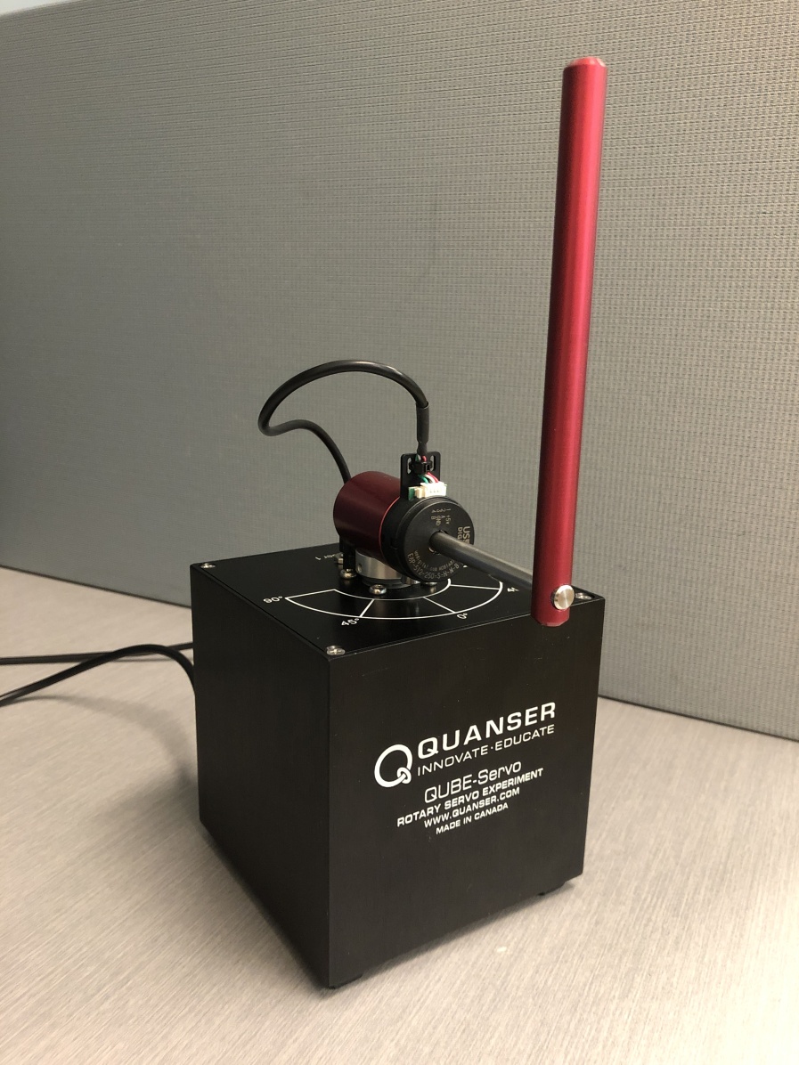
Figure 4: The Quanser QUBE-Servo system used to demonstrate the proposed closed-loop Koopman operator approximation method.

IV-A Experimental setup

The QUBE-Servo has one DC motor with a maximum input voltage of $10\text{\,}\mathrm{V}$, as well as two incremental encoders with $\mathrm{2}\mathrm{0}\mathrm{4}\mathrm{8}$ counts per revolution. The system is controlled by two parallel proportional-derivative controllers that track references for the motor angle $x_{1}^{\mathrm{p}}(t)$ and the pendulum angle $x_{2}^{\mathrm{p}}(t)$. The reference signals are denoted $r_{1}(t)$ and $r_{2}(t)$, while the feedforward is denoted $f(t)$. All angles are presented in radians, while the plant inputs are presented in Volts.

The controller’s transfer matrix from tracking error ${\mbf{e}(t)=\mbf{r}(t)-\mbf{x}^{\mathrm{p}}(t)}$ to output $\upsilon^{\mathrm{p}}(t)$ is

$$\mbf{K}(s)=\begin{bmatrix}K_{1}^{\mathrm{p}}+K_{1}^{\mathrm{d}}\frac{as}{s+a}&K_{2}^{\mathrm{p}}+K_{2}^{\mathrm{d}}\frac{as}{s+a}\end{bmatrix},$$ (69)

where $K_{1}^{\mathrm{p}}=6$ and $K_{2}^{\mathrm{p}}=30$ are the proportional gains, $K_{1}^{\mathrm{d}}=1.8$ and $K_{2}^{\mathrm{d}}=2.5$ are the derivative gains, and $a=$50\text{\,}\mathrm{Hz}$$ is the derivative filter cutoff frequency. The controller is discretized using the zero-order hold with a sampling frequency of $500\text{\,}\mathrm{Hz}$.

Samples of the exogenous test inputs are pictured in Figure 5. The motor angle reference signal is an integrated pseudorandom binary sequence, while the pendulum angle reference and feedforward signals are pseudorandom binary sequences [21, §13.3]. The pseudorandom binary sequences are smoothed using a low-pass filter with a cutoff frequency of $200\text{\,}\mathrm{Hz}$. The signal amplitudes excite the rotary inverted pendulum as much as possible without causing the pendulum to fall from its upright position.

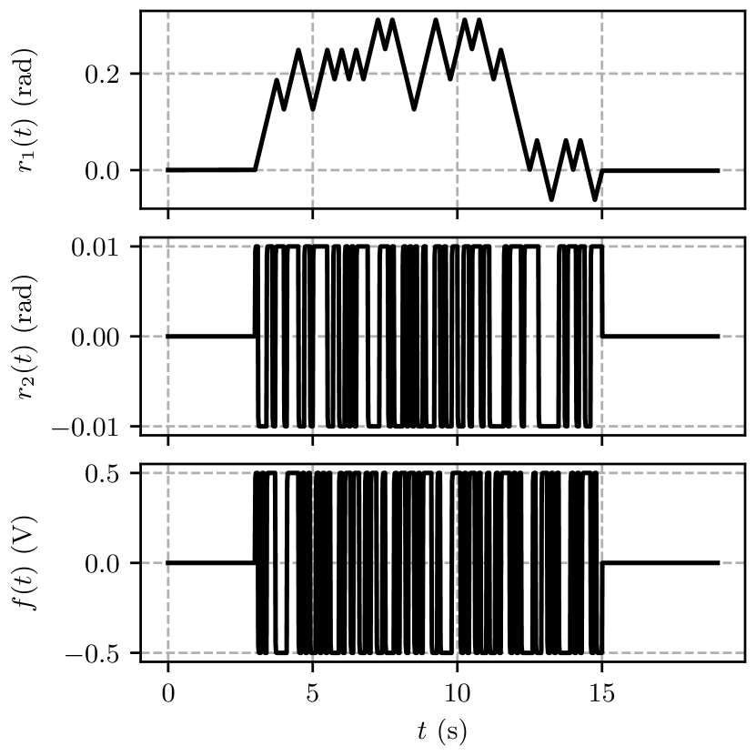
Figure 5: Sample of the exogenous test inputs used to identify a Koopman model of the Quanser QUBE-Servo.

The dataset presented here consists of $30$ training episodes and $20$ test episodes. Each episode is $20\text{\,}\mathrm{s}$, or $10\,000$ samples, long. The motor angle, pendulum angle, motor voltage, reference motor angle, reference pendulum angle, and feedforward voltage are recorded at every timestep. The controller’s state is computed at each timestep using the recorded tracking error. The first $1\text{\,}\mathrm{s}$ of each dataset is discarded to remove the transients associated with manually raising the pendulum to the upright position.

The Koopman lifting functions chosen for the rotary inverted pendulum are second order monomials followed by $10$ time delays. As required by the proposed method, the inputs and controller states are not lifted. Further performance improvement can be achieved by including more time delays, with diminishing returns after $20$.

The software required to fully reproduce the results of this paper, including the QUBE-Servo dataset, is available at https://github.com/decargroup/closed_loop_koopman. This code extends pykoop [34], the authors’ open source Koopman operator approximation library for Python. The software used to gather the QUBE-Servo dataset, implemented in C, is available at https://github.com/decargroup/quanser_qube.

IV-B Comparison of regularization methods and scoring metrics

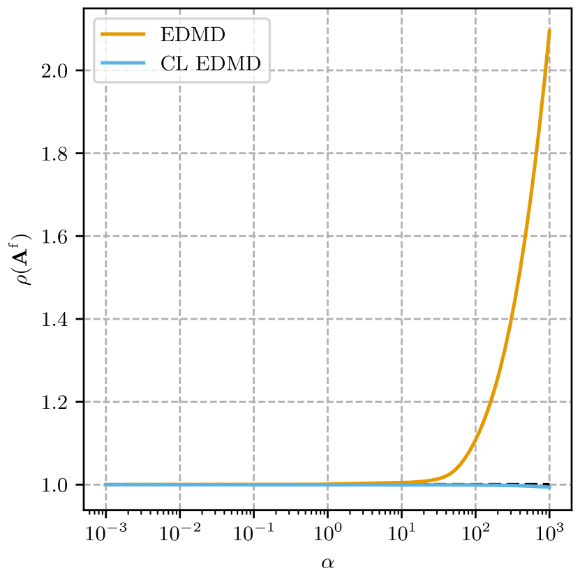
(a) Relationship between the regularization coefficient $\alpha$ and the spectral radii of the closed-loop systems identified with EDMD and closed-loop EDMD. As $\alpha$ increases, the closed-loop system identified with EDMD becomes unstable, while the closed-loop system identified with the proposed method remains asymptotically stable.

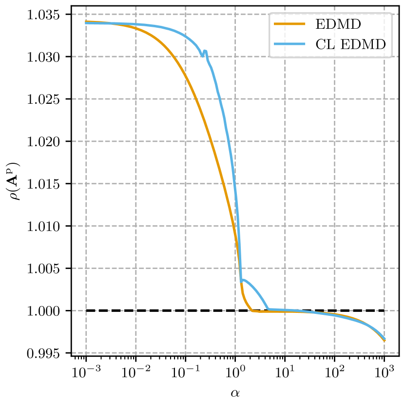
(b) Relationship between the regularization coefficient $\alpha$ and the spectral radii of the plant systems identified with EDMD and closed-loop EDMD. As $\alpha$ increases, both plant systems are incorrectly stabilized by the regularization.

Figure 6: Relationships between the regularization coefficients and the spectral radii of the closed-loop and plant systems.

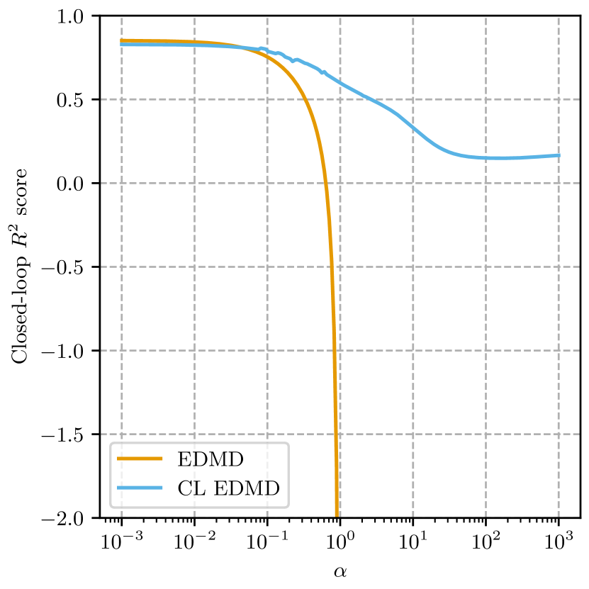
(a) Relationship between the regularization coefficient $\alpha$ and the test set $R^{2}$ scores of the closed-loop systems identified with EDMD and closed-loop EDMD. As $\alpha$ increases, both scores decrease. However, the system identified with EDMD becomes unstable around $\alpha=1$, and its prediction score diverges.

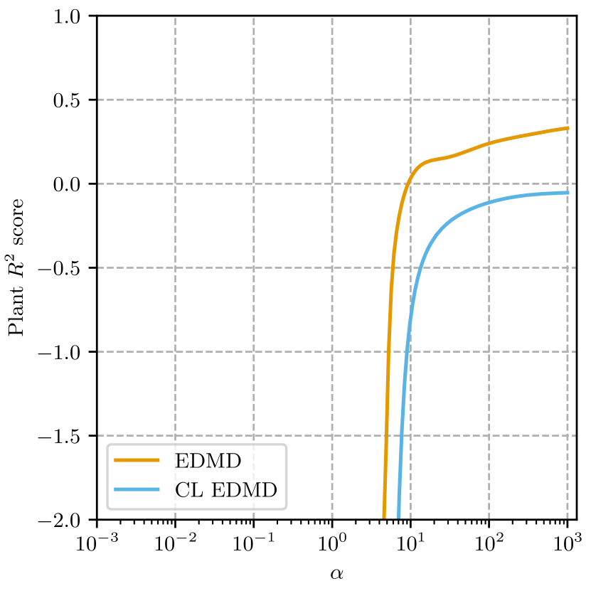
(b) Relationship between the regularization coefficient $\alpha$ and the test set $R^{2}$ scores of the plant systems identified with EDMD and closed-loop EDMD. The plant prediction scores are only finite for large regularization coefficients, indicating that is not a good metric for tuning the regularizer.

Figure 7: Relationships between the regularization coefficients and the test set $R^{2}$ scores of the closed-loop and plant systems.

Since the QUBE-Servo dataset does not contain significant sensor noise, Extended DMD does not identify a noticeably biased Koopman model. In fact, with no regularization, both EDMD and the proposed closed-loop method identify the same Koopman system. However, in many situations, regularization is a necessary component of the Koopman identification process. Choosing an appropriate regularization coefficient typically requires a hyperparameter optimization procedure. As such, the advantages of the proposed method are examined through the lens of hyperparameter optimization.

The proposed closed-loop Koopman operator approximation method is first compared to EDMD by varying the regularization coefficient $\alpha$ of each identification method. Specifically, $\mathrm{1}\mathrm{8}\mathrm{0}$ values of $\alpha$ are evaluated, spaced logarithmically between $10^{-3}$ and $10^{3}$. Recall that EDMD with Tikhonov regularization penalizes the squared Frobenius norm of the plant system, $\|\mbf{U}^{\mathrm{p}}\|_{\mathsf{F}}^{2}$, while the proposed closed-loop method penalizes the squared Frobenius norm of the closed-loop system, $\|\mbf{U}^{\mathrm{f}}\|_{\mathsf{F}}^{2}$. For the sake of comparison with the closed-loop approach, the open-loop plant models identified by EDMD are wrapped with the known controller. Since the proposed approach simultaneously identifies the closed-loop and plant systems, the plant system identified using the proposed method can be compared directly to the plant model identified using EDMD.

As a first point of comparison between EDMD and the proposed closed-loop method, consider the spectral radii of the closed-loop and plant systems as a function of their regularization coefficients. Given prior knowledge of the inverted pendulum system, both in open-loop and closed-loop contexts, a desirable Koopman model should have asymptotically stable closed-loop dynamics when controlled using an appropriate controller, but unstable open-loop dynamics. Figure 6(a) shows that regularizing using the Koopman matrix of the closed-loop system always results in an asymptotically stable closed-loop system. However, regularizing using the plant’s Koopman matrix results in an unstable closed-loop system for high enough regularization coefficients. According to Figure 6(b), the spectral radii of the plant systems identified with both methods share a similar trend. For low regularization coefficients, the systems are correctly identified as unstable, while for very high regularization coefficients, the plant systems are incorrectly stabilized. Both plots in Figure 6 indicate that a low regularization coefficient is appropriate for this system.

As a second point of comparison between the EDMD and the proposed method, consider the three-fold cross-validation score associated with each regularization coefficient. A good cross-validation score should reach its maximum at an appropriate hyperparameter value for the system. Given the spectral radius results in Figure 6, a good scoring metric for the QUBE-Servo system should have its peak at a low regularization coefficient. The scoring metric of choice for this system is the $R^{2}$ score, also called the coefficient of determination [35]. The $R^{2}$ score of a predicted state trajectory $\hat{x}_{k}$ relative to the true state trajectory $x_{k}$ is

$$R^{2}(x_{k},\hat{x}_{k})=1-\frac{\sum_{k=1}^{q}{(x_{k}-\hat{x}_{k})}^{2}}{\sum_{k=1}^{q}{(x_{k}-\bar{x})}^{2}},$$ (70)

where $\bar{x}=\frac{1}{q}\sum_{k=1}^{q}x_{k}$ is the mean value of $x_{k}$. For multidimensional predicted trajectories, the $R^{2}$ score of each state is averaged to obtain a single score. Perfect predictions receive an $R^{2}$ score of $1$, while predictions that only capture the mean of the data receive an $R^{2}$ score of $0$. Worse predictions can receive arbitrarily negative scores.

As before, Figure 7(a) shows the closed-loop $R^{2}$ scores of models identified with both EDMD and the proposed method, where the plant model identified with EDMD is wrapped with the known controller. For any regularization coefficient, the $R^{2}$ score achieved by the proposed method remains bounded and positive. Thus, the closed-loop regularizer has the expected effect of driving the predicted trajectory towards the mean as the regularization coefficient grows. However, for a large enough regularization coefficient, EDMD identifies an unstable closed loop system and its $R^{2}$ score diverges. The best closed-loop $R^{2}$ scores for both methods are attained with a very small regularization, which also leads to the expected stability properties. The use of the plant’s open-loop predictions to score the models does not share this behaviour. Since the plant system is inherently unstable, its predictions are highly sensitive to small variations in parameters and initial conditions. Thus, even the predictions of an accurate model can yield unbounded prediction errors. As shown in Figure 7(b), the only way to achieve a finite plant $R^{2}$ score is to select an extremely large regularization coefficient. For EDMD, this results in an unstable closed-loop system and an asymptotically stable plant, which does not reflect the underlying dynamics of the inverted pendulum system. While the proposed closed-loop methods produces an asymptotically stable closed-loop system for all regularizers, the open-loop plant it identifies still becomes asymptotically stable for a large enough regularization coefficient.

Figures 6 and 7 demonstrate two key conclusions. First, the closed-loop prediction error should be used for assessing the accuracy of identified models, as the best closed-loop scores correspond to Koopman models with the expected stability properties. Second, regularizing the closed-loop Koopman matrix is preferable to regularizing only the plant’s Koopman matrix, as it ensures the closed-loop system will remain asymptotically stable for high regularization coefficients. Note that closed-loop scoring can be leveraged without the proposed method, simply by identifying the plant using EDMD and wrapping the resulting model with the known controller. However, this approach is susceptible to bias when significant sensor noise is present. Also, only the proposed closed-loop approach has access to the closed-loop Koopman matrix for regularization. Thus, if the controller is already known, it is preferable to use the proposed closed-loop approach from the beginning, rather than leveraging controller knowledge only at the end of the identification procedure.

IV-C Comparison of optimized regularization coefficients

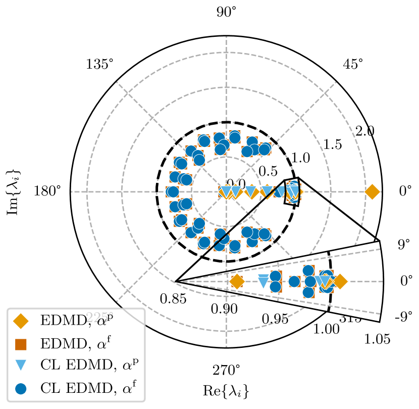
(a) Eigenvalues of the closed-loop systems identified with EDMD and closed-loop EDMD. Unlike EDMD, CL EDMD correctly identifies a stable closed-loop system for both regularization coefficients.

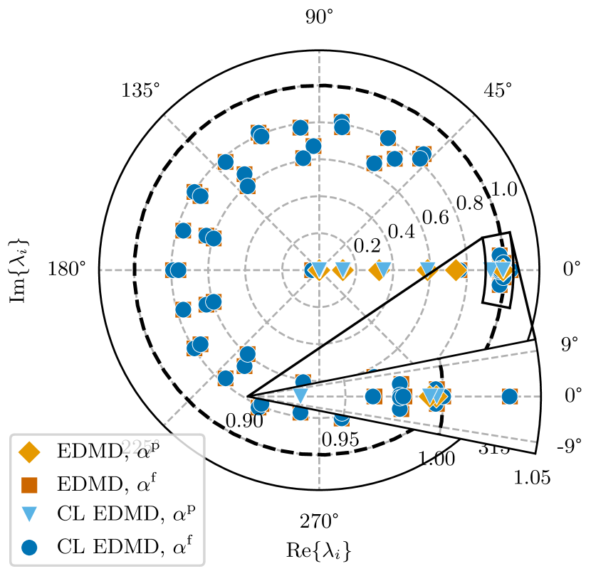
(b) Eigenvalues of the plant systems identified with EDMD and closed-loop EDMD. For small regularization coefficients, both EDMD and CL EDMD correctly identify unstable plant systems.

Figure 8: Eigenvalues of the closed-loop and plant systems.

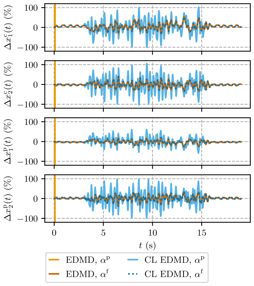
(a) Prediction errors of the closed-loop systems identified with EDMD and closed-loop EDMD. Unlike CL EDMD, EDMD incorrectly identifies an unstable closed-loop system when using a large regularization coefficient.

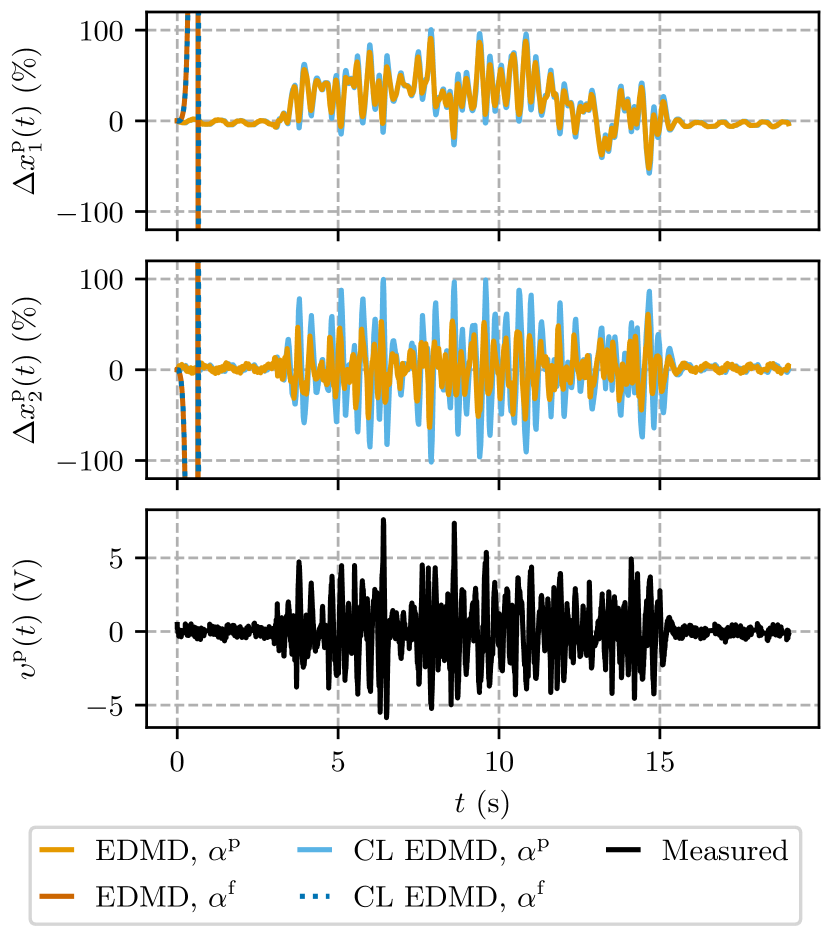
(b) Prediction errors and controller output of the plant systems identified with EDMD and closed-loop EDMD. Despite the diverging prediction errors, both methods correctly identify unstable plants for small regularization coefficients.

Figure 9: Prediction errors of the closed-loop and plant systems.

Informed by the results of Section IV-B, four approaches to identifying a Koopman model of the QUBE-Servo are compared via their eigenvalues and prediction errors. First is the naive open-loop approach, where EDMD is used to identify the plant’s Koopman matrix, and the regularization coefficient is selected according to the plant’s $R^{2}$ score. In this case, the optimal regularization coefficient is $\alpha^{\mathrm{p}}=10^{3}$. Second is another open-loop approach, where EDMD is used to identify the plant’s Koopman matrix, but the plant is then wrapped with the known controller and the regularization coefficient is selected according to the closed-loop system’s $R^{2}$ score. In this case, the optimal regularization coefficient is $\alpha^{\mathrm{f}}=10^{-3}$. Third is a closed-loop approach, where the closed-loop and plant’s Koopman matrices are simultaneously identified, but the plant’s $R^{2}$ score is used to select the regularization coefficient. In this case, the optimal regularization coefficient is $\alpha^{\mathrm{p}}=10^{3}$. Last is the proposed closed-loop approach, where the closed-loop and plant’s Koopman matrices are simultaneously identified, and the closed-loop $R^{2}$ score is used to select the regularization coefficient. In this case, the optimal regularization coefficient is $\alpha^{\mathrm{f}}=10^{-3}$.

Consider the closed-loop and plant eigenvalues in Figure 8. The naive approach, which uses the plant for regularization and scoring, identifies an unstable closed-loop system with two eigenvalues clearly outside the unit circle. Due to the large regularization coefficient, the plant system it identifies is asymptotically stable, which is also inconsistent with the underlying dynamics of the system. The third approach, which uses the closed-loop system for regularization but the plant for scoring, correctly identifies an asymptotically stable closed-loop system, but incorrectly identifies an asymptotically stable plant. The remaining two approaches, which use the closed-loop $R^{2}$ score to select the regularization coefficient, identify essentially the same eigenvalues. Both methods correctly identify asymptotically stable closed-loop systems and unstable plant systems. Since measurements from the QUBE-Servo system are relatively noiseless, it is expected that the two methods should agree. However, as is well-documented in the system identification literature, the closed-loop method could reduce the bias in the identified model in the presence of significant measurement noise [18, 19], [22, §11.1].

Looking at the closed-loop and plant prediction errors of each of these approaches in Figures 9(a) and 9(b) respectively tells the same story as the eigenvalues. Both EDMD and the proposed closed-loop method identify the same Koopman systems at low regularization coefficients. For large regularization coefficients, EDMD incorrectly identifies an unstable closed-loop system and an asymptotically stable plant. However, the proposed method identifies an asymptotically stable closed-loop system, regardless of the regularization coefficient. The $R^{2}$ scores and normalized root-mean-squared errors (NRMSE) of each model on the test set are summarized in Table I. To compute the NRMSE, the root-mean-squared error of each state is normalized by the peak amplitude of the true value of that state. The normalized values for each state are then averaged to obtain a single number summarizing the error of the trajectory prediction.

TABLE I: $R^{2}$ score and NRMSE over $20$ test episodes.

Reg.	Score	$R^{2}$ avg.	$R^{2}$ std.	NRMSE avg.	NRMSE std.
Plant	Plant	$-\infty$	—	$\infty$	—
Plant	CL	$0.845$	$0.020$	$10.9\text{\,}\mathrm{\char 37\relax}$	$1.0\text{\,}\mathrm{\char 37\relax}$
CL	Plant	$0.124$	$0.030$	$26.2\text{\,}\mathrm{\char 37\relax}$	$2.1\text{\,}\mathrm{\char 37\relax}$
CL	CL	$0.840$	$0.018$	$11.1\text{\,}\mathrm{\char 37\relax}$	$0.9\text{\,}\mathrm{\char 37\relax}$

Table I shows that the most important factor for attaining a high prediction score is the use of the closed-loop prediction error for scoring. For the QUBE-Servo system, the choice to use the closed-loop or plant Koopman matrix for regularization is not critical, as long as a sufficiently small regularization coefficient is chosen. However, it must be noted that identifying the open-loop plant directly with EDMD and wrapping the model with the known controller for scoring requires knowledge of the controller and measurements of the controller output, which may not be available. If knowledge of the controller is already assumed, then using the proposed closed-loop method is preferable, as it avoids the possibility of bias in the models. Furthermore, in the proposed closed-loop Koopman operator approximation approach both $\mbf{U}^{\mathrm{f}}$ and $\mbf{U}^{\mathrm{p}}$ are available as optimization variables. This additional flexibility allows additional knowledge of the closed-loop system and plant to be incorporated into the optimization problem. For example, the closed-loop system could be constrained to be asymptotically stable [23]. Alternatively, known properties of the closed-loop system or plant could be incorporated by constraining the poles to a particular region [36]. The advantages and disadvantages of each approach are summarized in Table II.

TABLE II: Comparison of Koopman ID methods

Reg.	Score	Bounded score?	CL reg.?	Avoids bias?
Plant	Plant	✗	✗	✗
Plant	CL	✓	✗	✗
CL	Plant	✗	✓	✓
CL	CL	✓	✓	✓

V Conclusion

When identifying closed-loop systems, it is often not possible to neglect the effects of the control loop. This holds true for Koopman operator approximation as well as linear system identification. In this paper, a closed-loop Koopman operator identification method is presented, where the closed-loop system and plant system are identified simultaneously using knowledge of the controller. The advantages of this method is demonstrated experimentally using an unstable rotary inverted pendulum system. In particular, the proposed closed-loop method identifies Koopman models that align with the prior knowledge that the closed-loop system is asymptotically stable, while the plant is unstable. The closed-loop method also naturally allows the closed-loop prediction error to be used as a goodness-of-fit metric, which is crucial for selecting lifting functions and an appropriate regularization coefficient. Finally, the proposed closed-loop Koopman operator approximation method allows both the closed-loop and plant Koopman matrices to be used in regularizers or constraints. Using Extended DMD, only the plant’s Koopman matrix can be used in a regularizer, leading to potentially unstable closed-loop systems for large regularization coefficients. The additional flexibility provided by the proposed closed-loop Koopman operator approximation method will be explored in future work, as the ability to incorporate known information about the closed-loop system or plant into the regression problem could prove useful in identifying more accurate or useful Koopman models. Extensions to address the use of nonlinear controllers, or to address the situation where the controller is also unknown could also prove valuable in broadening the applicability of the proposed method.

[Recovery of the plant using least-squares]

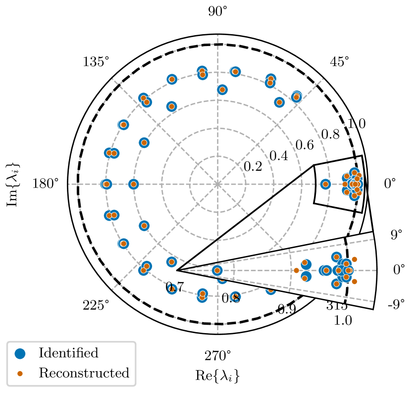
(a) Closed-loop eigenvalues identified with the least-squares version of CL EDMD, before and after the plant is extracted and the controller is re-connected. When the closed-loop system is reconstructed from the plant, the eigenvalues move, and some of them leave the unit circle, making the closed-loop system unstable.

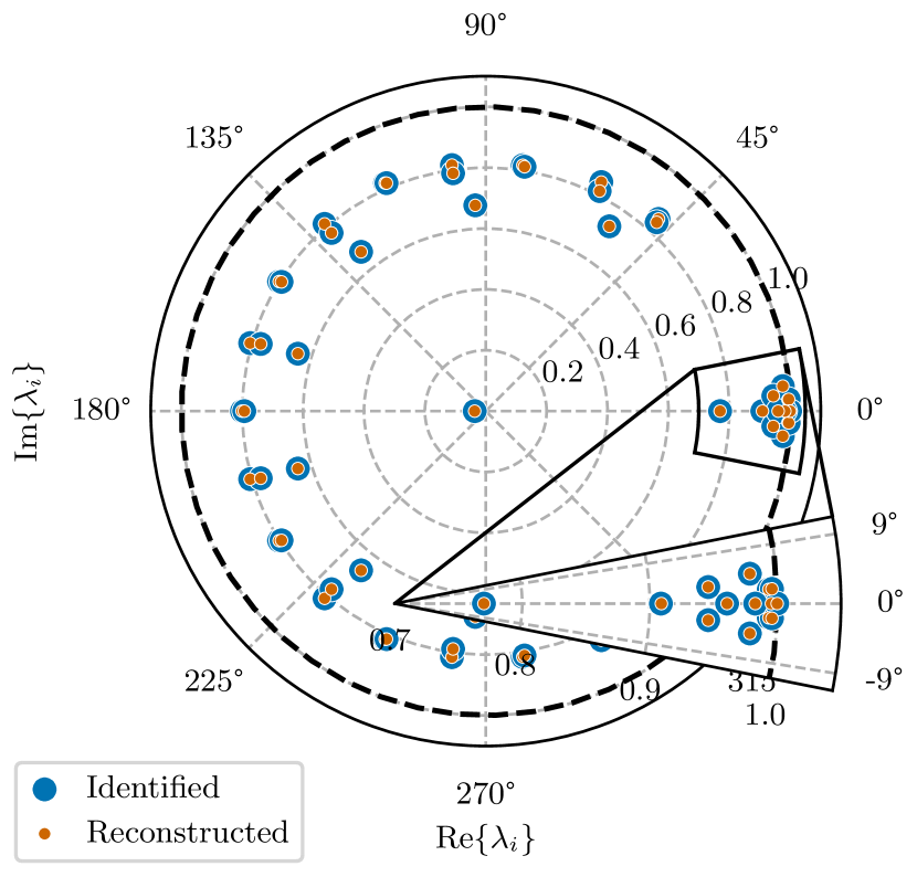
(b) Closed-loop eigenvalues identified with the constrained version of CL EDMD, before and after the plant is extracted and the controller is re-connected. When the closed-loop system is reconstructed from the plant, the eigenvalues do not change, indicating that the constrained regression procedure respects the structure of the closed-loop system.

Figure 10: Closed-loop eigenvalues identified with the least-squares and constrained versions of CL EDMD.

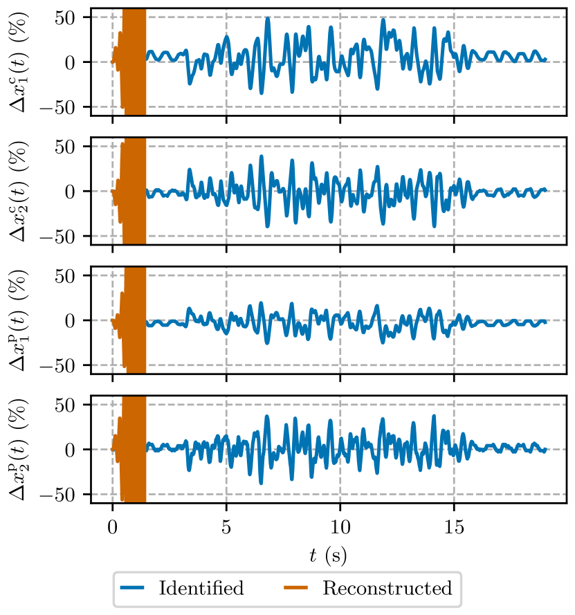
(a) Closed-loop prediction errors of models identified with the least-squares version of CL EDMD, before and after the plant is extracted and the controller is re-connected. Reconstructing the closed-loop system destabilizes it, as indicated by the diverging predictions of the reconstructed model.

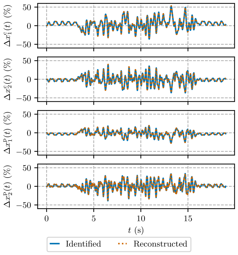
(b) Closed-loop prediction errors of models identified with the constrained version of CL EDMD, before and after the plant is extracted and the controller is re-connected. Reconstructing the closed-loop system does not change its predictions, indicating that the constrained regression procedure respects its structure.

Figure 11: Closed-loop prediction errors of models identified with the least-squares and constrained versions of CL EDMD.

Using least-squares to extract a plant model from an identified closed-loop system seems to provide a simpler alternative to the constraint-based formulation in (53)–(55). However, using (51) and (52) to obtain a Koopman model of the plant does not respect the feedback structure of the system. In fact, extracting the plant from the closed-loop system and re-wrapping it with the same controller does not result in the same system. Figure 10(a) shows how the closed-loop eigenvalues change when the plant is extracted and re-wrapped with a controller. In this case, the procedure actually destabilizes the system. When using the constraint-based approach, as shown in Figure 10(b), extracting the plant and closing the loop again with the same controller does not move the eigenvalues. Figure 11 shows the prediction errors of each system before and after removing and re-adding the controller. As expected, the predicted trajectories of the destabilized system diverge quickly. The ability to extract the plant from the closed-loop system while respecting the feedback structure of the system is particularly important for control design tasks, where, presumably, the plant is being identified with the end goal of designing an improved controller.

References

- [1] B.. Koopman “Hamiltonian systems and transformations in Hilbert space” In Proc. Nat. Acad. Sci. 17.5, 1931, pp. 315–318 DOI: 10.1073/pnas.17.5.315
- [2] Igor Mezić “Spectrum of the Koopman Operator, Spectral Expansions in Functional Spaces, and State-Space Geometry” In J. Nonlinear Sci. 30.5, 2019, pp. 2091–2145 DOI: 10.1007/s00332-019-09598-5
- [3] Marko Budišić, Ryan Mohr and Igor Mezić “Applied Koopmanism” In Chaos 22.4, 2012 DOI: 10.1063/1.4772195
- [4] “The Koopman Operator in Systems and Control” Cham, Switzerland: Springer, 2020 DOI: 10.1007/978-3-030-35713-9
- [5] Ian Abraham and Todd D. Murphey “Active Learning of Dynamics for Data-Driven Control Using Koopman Operators” In IEEE Trans. Robot. 35.5, 2019, pp. 1071–1083 DOI: 10.1109/tro.2019.2923880
- [6] Giorgos Mamakoukas, Maria Castano, Xiaobo Tan and Todd Murphey “Local Koopman Operators for Data-Driven Control of Robotic Systems” In Proc. Robot.: Sci. Syst. XV, 2019 DOI: 10.15607/RSS.2019.XV.054
- [7] Daniel Bruder, Brent Gillespie, C. Remy and Ram Vasudevan “Modeling and Control of Soft Robots Using the Koopman Operator and Model Predictive Control” In Proc. Robot.: Sci. Syst. XV, 2019 DOI: 10.15607/rss.2019.xv.060
- [8] Ian Abraham, Gerardo Torre and Todd Murphey “Model-Based Control Using Koopman Operators” In Proc. Robot.: Sci. Syst. XIII, 2017 DOI: 10.15607/rss.2017.xiii.052
- [9] Zi Cong Guo, Vassili Korotkine, James R. Forbes and Timothy D. Barfoot “Koopman Linearization for Data-Driven Batch State Estimation of Control-Affine Systems” In IEEE Robotics and Automation Letters 7.2, 2022, pp. 866–873 DOI: 10.1109/LRA.2021.3133587
- [10] Anthony M. DeGennaro and Nathan M. Urban “Scalable Extended Dynamic Mode Decomposition Using Random Kernel Approximation” In SIAM J. Sci. Comput. 41.3 Society for Industrial & Applied Mathematics (SIAM), 2019, pp. A1482–A1499
- [11] Ali Rahimi and Benjamin Recht “Random Features for Large-Scale Kernel Machines” In Proc. 20th Int. Conf. Neural Inf. Process. Syst., NeurIPS’07 Vancouver, Canada: Curran Associates Inc., 2007, pp. 1177–1184
- [12] Milan Korda and Igor Mezić “Linear predictors for nonlinear dynamical systems: Koopman operator meets model predictive control” In Automatica 93, 2018, pp. 149–160 DOI: 10.1016/j.automatica.2018.03.046
- [13] Shaowu Pan and Karthik Duraisamy “On the structure of time-delay embedding in linear models of non-linear dynamical systems” In Chaos 30.7 AIP Publishing, 2020 DOI: 10.1063/5.0010886
- [14] Samuel E. Otto and Clarence W. Rowley “Koopman Operators for Estimation and Control of Dynamical Systems” In Annu. Rev. Control, Robot., Auton. Syst. 4.1, 2021, pp. 59–87 DOI: 10.1146/annurev-control-071020-010108
- [15] Daisuke Uchida, Atsushi Yamashita and Hajime Asama “Data-Driven Koopman Controller Synthesis Based on the Extended Norm Characterization” In IEEE Contr. Syst. Lett. 5.5, 2021, pp. 1795–1800 DOI: 10.1109/lcsys.2020.3042827
- [16] Lennart Ljung, Tianshi Chen and Biqiang Mu “A shift in paradigm for system identification” In Int. J. Control 93.2 Informa UK Ltd., 2019, pp. 173–180
- [17] Steven L. Brunton, Marko Budišić, Eurika Kaiser and J. Kutz “Modern Koopman Theory for Dynamical Systems” In SIAM Review 64.2 Society for Industrial & Applied Mathematics (SIAM), 2022, pp. 229–340 DOI: 10.1137/21m1401243
- [18] Urban Forssell and Lennart Ljung “Closed-loop identification revisited” In Automatica 35.7 Elsevier BV, 1999, pp. 1215–1241 DOI: 10.1016/s0005-1098(99)00022-9
- [19] Paul Van Hof “Closed-loop issues in system identification” In Annual Reviews in Control 22 Elsevier BV, 1998, pp. 173–186 DOI: 10.1016/s1367-5788(98)00016-9
- [20] P. Van Overschee and B. De Moor “Closed loop subspace system identification” In Proc. 36th IEEE Conf. Decis. Control, 1997
- [21] Lennart Ljung “System Identification: Theory for the User” Prentice Hall, 1999
- [22] Tohru Katayama “Subspace Methods for System Identification” Springer, 2005 DOI: 10.1007/1-84628-158-x
- [23] Steven Dahdah and James R. Forbes “System norm regularization methods for Koopman operator approximation” In Proc. R. Soc. A 478.2265 The Royal Society, 2022 DOI: 10.1098/rspa.2022.0162
- [24] Nathan J. Kutz, Steven L. Brunton, Bingni W. Brunton and Joshua L. Proctor “Dynamic Mode Decomposition: Data-Driven Modeling of Complex Systems” Philadelphia, PA: SIAM, 2016 DOI: 10.1137/1.9781611974508
- [25] Daniel Bruder, Xun Fu and Ram Vasudevan “Advantages of Bilinear Koopman Realizations for the Modeling and Control of Systems With Unknown Dynamics” In IEEE Trans. Robot. Autom. 6.3, 2021, pp. 4369–4376 DOI: 10.1109/lra.2021.3068117
- [26] Michael Green and David J.. Limebeer “Linear Robust Control” London, England: Prentice Hall, 1994
- [27] Matthew O. Williams, Ioannis G. Kevrekidis and Clarence W. Rowley “A Data–Driven Approximation of the Koopman Operator: Extending Dynamic Mode Decomposition” In J. Nonlinear Sci. 25.6, 2015, pp. 1307–1346 DOI: 10.1007/s00332-015-9258-5
- [28] A.. Tikhonov, A. Goncharsky, V.. Stepanov and A.. Yagola “Numerical Methods for the Solution of Ill-Posed Problems” Dordrecht, Netherlands: Springer, 1995 DOI: 10.1007/978-94-015-8480-7
- [29] Sigurd Skogestad and Ian Postlethwaite “Multivariable Feedback Control: Analysis and Design” John Wiley & Sons, 2006
- [30] Steven Dahdah and James Richard Forbes “Linear Matrix Inequality Approaches to Koopman Operator Approximation” In arXiv:2102.03613v2 [eess.SY], 2021
- [31] Ryan James Caverly and James Richard Forbes “LMI Properties and Applications in Systems, Stability, and Control Theory” In arXiv:1903.08599v3 [cs.SY], 2019
- [32] Scott T.. Dawson, Maziar S. Hemati, Matthew O. Williams and Clarence W. Rowley “Characterizing and correcting for the effect of sensor noise in the dynamic mode decomposition” In Exp. Fluids 57.3 Springer, 2016
- [33] Quanser “QUBE-Servo 2”, 2023 URL: https://www.quanser.com/products/qube-servo-2/
- [34] Steven Dahdah and James Richard Forbes “decargroup/pykoop” Zenodo, 2023 DOI: 10.5281/zenodo.7464660
- [35] Sewall Wright “Correlation and causation” In J. Agricultural Res. 20, 1921, pp. 557–585
- [36] M. Chilali, P. Gahinet and P. Apkarian “Robust pole placement in LMI regions” In IEEE Trans. Autom. Control 44.12 Institute of ElectricalElectronics Engineers (IEEE), 1999, pp. 2257–2270