2023 043 16 March

Material budget weights

ALICE Collaboration ALICE Collaboration

The knowledge of the material budget with a high precision is fundamental for measurements of direct photon production using the photon conversion method due to its direct impact on the total systematic uncertainty. Moreover, it influences many aspects of the charged-particle reconstruction performance. In this article, two procedures to determine data-driven corrections to the material-budget description in ALICE simulation software are developed. One is based on the precise knowledge of the gas composition in the Time Projection Chamber. The other is based on the robustness of the ratio between the produced number of photons and charged particles, to a large extent due to the approximate isospin symmetry in the number of produced neutral and charged pions. Both methods are applied to ALICE data allowing for a reduction of the overall material budget systematic uncertainty from 4.5% down to 2.5%. Using these methods, a locally correct material budget is also achieved. The two proposed methods are generic and can be applied to any experiment in a similar fashion.

1 Introduction

The ALICE experiment is a dedicated heavy-ion experiment at the CERN LHC [1, 2, 3]. In ALICE, photons are measured using either the calorimeters (PHOS [4, 5], EMCal [6, 7, 8]), or the Photon Conversion Method (PCM) [9, 2], i.e. via the reconstruction of e⁺e^- pairs from photon conversions in the detector material. The material budget is, expressed in % of radiation lengths, $X/X_{\mathrm{0}}=$ (11.4 $\pm$ 0.5)% [9, 2]. This value is an average over the pseudorapidity range $|\eta|<0.9$ and it is integrated in the radial direction ($R$) up to 180 cm, where $R$ is calculated in the transverse $xy$-plane to the beam axis ($z$). This uncertainty in the material budget translates into a systematic uncertainty of photon spectrum measurements. For example, direct-photon production was measured in Pb–Pb collisions at a center of mass energy per nucleon pair of $\sqrt{s_{\mathrm{NN}}}$ $=$ 2.76 TeV in three centrality classes by ALICE [10]. The measurement was done by a combination of the independent PCM and PHOS measurements. A low transverse momentum ($p_{\rm T}$) excess with respect to perturbative Quantum Chromodynamics (pQCD) prompt-photon predictions is observed, which can be attributed to thermal photon emission from the quark–gluon plasma (QGP). The current uncertainties do not allow for discrimination among the proposed theoretical models [11, 12, 13, 14, 15, 16, 17, 18, 19]. For the events in the 0–20% centrality interval, the low $p_{\rm T}$ excess is of the order of 10–15%, and the total uncertainty is approximately 6% at low $p_{\rm T}$ with the largest contribution being the 4.5% of the material budget. Therefore, reducing the uncertainty of the material budget is essential for improving the significance of the direct-photon measurements and, thereby, allowing for a larger discrimination power among the different theoretical models.

The estimated systematic uncertainty related to the material budget of $\pm 4.5$% [9, 2] is an average over the $R$ range given above. Initially, the systematic uncertainty was estimated by comparing the reconstructed number of $\gamma$ conversions ($N_{\rm{\gamma}}$) normalized to the number of charged particles ($N_{\rm{\gamma}}/N_{\rm{\tiny ch}}$) between real data (RD) and Monte Carlo (MC) simulations. Two event generators (PYTHIA 6 [20] and PHOJET 1.12 [21]), two secondary vertex finder algorithms with different optimization criteria, and two momentum ranges were considered. Local differences of up to 20% were observed in some parts of the detector. The development of new procedures to reduce the systematic uncertainty and to achieve a more accurate local description of the material budget in the simulation is therefore mandatory.

This article establishes two data-driven correction methods for a precise determination of the material budget of a given detector using reconstructed photon conversions. The methods are based either on the existence of a well-known piece of material (e.g. the TPC gas in the ALICE case) or on the robustness of the ratio $N_{\rm{\gamma}}/N_{\rm{\tiny ch}}$ above a low $p_{\rm T}$ threshold which is largely due to the approximate isospin symmetry in pion production. The two methods are developed for the ALICE experiment but can, in principle, be employed in any other experiment.

This article is organized as follows. The ALICE experimental setup and event sample used in this article and the photon reconstruction are described in Sec. 2, and Sec. 3, respectively. The proposed correction procedures are introduced in Sec. 4. The results are presented in Sec. 5 followed by the conclusions in Sec. 6.

2 Detector description and data sample

A comprehensive description of the ALICE experiment during the LHC Runs 1 and 2 and its performance can be found in Refs. [1, 2]. The relevant detectors for this analysis are the Inner Tracking System (ITS) [22], the Time Projection Chamber (TPC) [23] and the V0 detectors[24] which are operated inside a magnetic field up to 0.5 T directed parallel to the beam axis. The ITS consists of six cylindrical layers of high resolution silicon tracking detectors. The two innermost layers located at a radial distance of 3.9 cm and 7.6 cm are silicon pixel detectors (SPD); the two intermediate layers are silicon drift detectors (SDD) positioned at 15.0 cm and at 23.9 cm; and the two outermost layers are silicon strip detectors (SSD) at 38.0 cm and 43.0 cm. It measures the position of the primary collision vertex, the impact parameter of the tracks, and improves considerably the track $p_{\rm T}$ resolution at high $p_{\rm T}$. The SDD and SSD layers provide the amplitude of the charged signal that is used for particle identification through the measurement of the specific energy loss ($\textrm{d}E/\textrm{d}x$). The TPC is a large ($\sim$ 85 m³) cylindrical drift detector filled during 2017 with a Ne/CO₂/N₂ (90/10/5) gas mixture. It covers a pseudorapidity acceptance of $|\eta|<0.9$ over the full azimuthal range, with a maximum of 159 reconstructed space points along the path of the track. In addition to the space points for the track reconstruction, the TPC provides particle identification via the measurement of the $\textrm{d}E/\textrm{d}x$. The V0 detector, which is made of two arrays of 32 plastic scintillators located at $2.8<\eta<5.1$ (V0A) and $-3.7<\eta<-1.7$ (V0C), is used for triggering on the collisions [24].

The analyses presented here use the low intensity part (up to few hundred Hz interaction rate) of the data recorded in 2017 during the LHC pp run at $\sqrt{s}$ = 5.02 TeV. A total of about 4 $\times$ 10⁷ pp collisions recorded with a minimum-bias (MB) trigger are used. The MB trigger was defined by signals in both V0 detectors in coincidence with a bunch crossing to minimize the contribution from diffractive interactions. Contamination from beam-induced background events, produced outside the interaction region, is removed using the timing information of the V0 detectors and taking into account the correlation between tracklets and clusters in the SPD detector [2]. The events used for the analysis are required to have a primary vertex in the fiducial region $|z|<10$ cm along the beam-line direction. The primary vertex is reconstructed either using global tracks (with ITS and TPC information) or using SPD tracklets. The contamination from in-bunch pile-up events is removed offline by excluding events with multiple vertices reconstructed in the SPD [25].

In general, MC simulations use a geometrical model of the ALICE detectors, an event generator as input, and a particle transport software, GEANT3[26] in the ALICE case.

3 Photon reconstruction

Photons are reconstructed by measuring the e⁺e^- pairs produced in photon conversions in the detector material. Charged tracks are reconstructed in the ALICE central barrel with the ITS [22] and the TPC [23], working together or independently. Two secondary-vertex algorithms with different optimization criteria are used in this analysis to search for oppositely-charged track pairs originating from a common (secondary) vertex, referred to as V⁰ [2]. The V⁰ sample consists mainly of ${\rm K}^{0}_{\rm{S}}$, $\Lambda$, $\overline{\Lambda}$ decays and $\gamma$ conversions. Selection criteria based on track quality, particle identification and the topology of a photon conversion are applied. The complete list of selection criteria is summarized in Table 1. Electrons, positrons, and photons are required to be within $|\eta|<$ 0.8. In order to ensure good track quality, a minimum track transverse momentum of 50 MeV/$c$ and a fraction of TPC clusters over findable clusters (the number of geometrically possible clusters which can be assigned to a track) above 0.6 were required. The conversion point of the photon candidates should be inside the $\eta$ acceptance and the conversion radius should be inside 0 $<R<$ 180 cm and within the limits given by the so called ‘line cut’ (see Table 1) to ensure that the photons come from the primary vertex. Electron identification and pion rejection are performed by using the specific energy loss $\textrm{d}E/\textrm{d}x$ in the TPC. The selection and rejection criteria are based on the number of standard deviations ($n\sigma_{e}$ and $n\sigma_{\pi}$ ) around the electron and pion hypothesis, where $\sigma$ is the standard deviation of the energy loss measurement. The remaining contamination from $\Lambda$, $\overline{\Lambda}$, and ${\rm K}^{0}_{\rm{S}}$ is further reduced using a two-dimensional selection in the ($\alpha$, $q_{\rm T}$) distribution, known as the Armenteros-Podolanski plot [27]; $\alpha$ is the longitudinal momentum asymmetry of positive and negative daughter tracks, defined as $\alpha=(p_{\mathrm{L}}^{+}-p_{\mathrm{L}}^{-})/(p_{\mathrm{L}}^{+}+p_{\mathrm{L}}^{-})$, and $q_{\rm T}$ is the transverse momentum of the decay particles with respect to the V⁰ momentum.

Table 1: Selection criteria applied to the V⁰ sample to select photons among the different particles.

Track reconstruction
e± track $p_{\rm T}$	$p_{\rm T}>0.05$ GeV/$c$
e± track $\eta$	$|\eta|<0.8$
$N_{\mbox{\tiny clusters}}/N_{\mbox{\tiny findable clusters}}$	$>60\%$
conversion radius	$0\,<\,R\,<\,180$ cm
line cut	$R>|Z|\times ZR_{\mbox{\tiny Slope}}-Z_{0}$
	with $ZR_{\mbox{\tiny Slope}}=\tan{(2\times\arctan(\exp(-\eta_{\mbox{\tiny cut}})))}$
	where $Z_{0}~{}=~{}$7 cm, $\eta_{\mbox{\tiny cut}}~{}=~{}$0.8
Track identification
$n\sigma_{\mathrm{e}}$ TPC	$-3<n\sigma_{\mathrm{e}}<5$
$n\sigma_{\pi}$ TPC	$n\sigma_{\pi}>2$ for $0.25<p<3.5$ GeV/$c$
	$n\sigma_{\pi}>0.5$ for $p>3.5$ GeV/$c$
Conversion $\gamma$ topology
$q_{\mbox{\tiny T}}$	$q_{\mbox{\tiny T}}<0.05\sqrt{1-(\alpha/0.95)^{2}}$ GeV/$c$
photon fit quality	$\chi^{2}_{\mbox{\tiny max}}=20$
$\psi_{\rm pair}$	$|\psi_{\rm pair}|<0.1\,(1-\chi^{2}/\chi^{2}_{\mbox{\tiny max}})$

Conversion electrons have a preferred emission orientation that can be described by the angle $\psi_{\mbox{\tiny pair}}$ between the plane that is perpendicular to the magnetic field (x-y plane) and the plane defined by the opening angle of the pair. A selection on $\psi_{\mbox{\tiny pair}}$ together with a cut on the photon $\chi^{2}$ of the Kalman filter fit [28] further suppresses the contamination from non-photonic V⁰ candidates. Monte Carlo simulations show that a photon purity above 99% is achieved at all transverse momenta except in the vicinity of $p_{\rm T}$ $\sim$ 0.3 GeV/$c$ where it decreases to 98%. Figure 1 shows the probability that a reconstructed electron carries a certain fraction of the photon energy ($x={{p_{\rm e}}/{p_{\gamma}}}$) for photon candidates below and above a momentum of 0.4 GeV/$c$. The RD as well as reconstructed distributions from a MC simulation based on PYTHIA 8 with the Monash 2013 tune [29, 30] as input event generator are shown. Converted photons with $p$ $>$ 0.4 GeV/$c$ can be reconstructed with electron fractional energies from 0 to 1, while at lower $p$ only largely symmetric conversions are detected. Differences between the data and MC distributions are largely due to different photon momentum distributions that are not yet equalized at this stage (see Eq. (14)). A high purity in the photon sample can be inferred from the similarity of the red points (MC) and blue curves that represent only MC verified photons (Fig. 1).

Figure 2 displays the radial distribution of photon conversion vertices. The experimental data as well as reconstructed distributions from a MC simulation based on PYTHIA 8 with the Monash 2013 tune [29, 30] as input event generator are shown. The radial distribution of reconstructed conversion vertices clearly reveals the different detector structures corresponding to the ITS and TPC. The experimental distribution is compared to the one obtained from MC simulations that accounts for the time-dependent variations of the detector conditions. The main goal is to select the primary photon sample, i.e. photons coming from electromagnetic decays of neutral mesons or direct photons. Additionally, there are three types of background contributions shown in the figure that need special treatment. i) Primary e⁺e^- pairs from $\pi^{0}$ (or $\eta$) Dalitz decays wrongly detected as conversion photons, mainly localized at radii smaller than 5 cm, can be suppressed by a minimum cut of 5 cm in the analysis. ii) Random combinatorial background, which is subtracted both in RD and MC based on the MC. iii) a 5–10% contribution of secondary photons [31] from weak decays of ${\rm K}^{0}_{\rm{S}}$ (e.g. ${\rm K}^{0}_{\rm{S}}$ $\rightarrow$$\pi^{0}$ $\pi^{0}$) and $\Lambda$ ($\overline{\Lambda}$) (e.g. $\Lambda$ $\rightarrow$n$\pi^{0}$) hadrons, and interactions in the detector material. The contribution from weak decays is estimated in the data by using a particle decay simulation called “cocktail simulation” [32] based on parametrizations of measured particle spectra, and in MC using the full MC information (labelled ‘True’ in Fig. 2 ). The contribution from interactions in the detector material is taken from MC, for both MC and real data (RD). The total secondary contribution is then subtracted from the photon sample in the data and in the MC simulated sample for each radial interval.

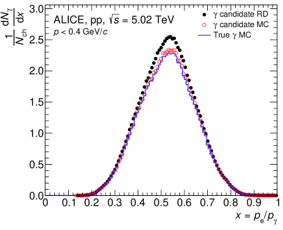
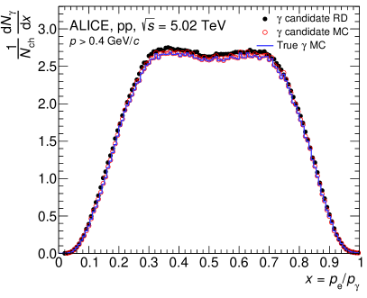
Figure 1: Distribution of the electron fractional energy ($x$) for photon candidates with $p<0.4$ GeV/$c$ (left) and with $p>0.4$ GeV/$c$ (right) reconstructed in real data (black points), in Monte Carlo simulations (red points), and for verified photons in MC simulations (blue lines) where PYTHIA8 is used as input event generator.

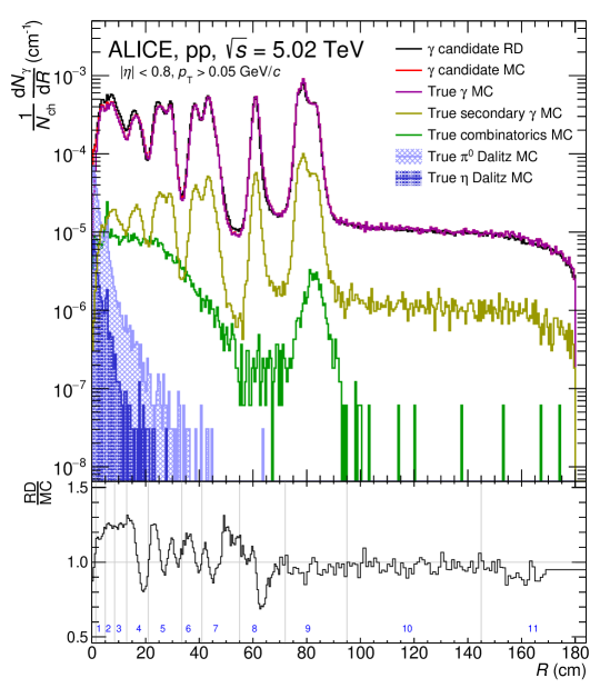
Figure 2: (Top) Radial distributions of reconstructed photon vertices in experimental data and in MC simulations are shown as black and red lines, respectively. Using the full MC information contributions from true photons (purple line), secondary photons (olive line), and combinatorial pairs (green line) are identified. The e⁺e^- pairs from $\pi^{0}$ (or $\eta$) Dalitz decays, wrongly identified as photon conversions, are depicted as blue shaded areas. (Bottom) Ratio of the radial distribution of reconstructed photon vertices in RD (black line) and MC (red line). Vertical lines in grey and blue numbers indicate the twelve radial intervals and their respective indices used in the analysis.

4 Calibration methods

The RD to MC comparison of the number of reconstructed photons as a function of the conversion point radius shown in Fig. 2 reveals local differences of up to 20% in the number of reconstructed photons. This provides evidence that the implementation of the material budget in the geometrical model of ALICE is not accurate enough in some parts of the detector, which may impact the precision of various analyses in ALICE.

Two data-driven calibration methods (the $\omega_{i}$ and ${\Omega}_{i}$ calibration weights, Sec. 4.1, Sec. 4.2 ) were developed in order to mitigate the differences by correcting the detector material description in MC simulations, and thus, reducing the systematic uncertainty. The complete radial range is subdivided in twelve intervals as shown in Fig. 2. The resulting calibration weights are then used to scale the photon reconstruction efficiency as follows:

$$\epsilon_{\gamma}^{\mathrm{MC,corr}}(p_{\mathrm{T}})=\frac{\sum\nolimits_{i}W_{i}\times\mathrm{d}N_{\gamma,i}^{\mathrm{rec,MC}}/\mathrm{d}p_{\mathrm{T}}}{\mathrm{d}N_{\gamma}^{\mathrm{prod}}/\mathrm{d}p_{\mathrm{T}}},$$ (1)

where $W_{\mathrm{i}}$ are the correction factors in each radial interval $i$ ($W_{i}\equiv\omega_{i}$ or $W_{i}\equiv{\Omega_{i}}$), d$N_{{\gamma,i}}^{\rm{\tiny rec,MC}}$/d$p_{\rm T}$ is the number of primary photons reconstructed in the Monte Carlo simulated data at a given $p_{\rm T}$ and radial interval $i$ (see Fig. 2) in the pseudorapidity range $|\eta|<0.8$, and d$N_{\rm{\gamma}}^{\rm{\tiny prod}}$/d$p_{\rm T}$ is the total number of photons produced at a given $p_{\rm T}$ as given by the input event generator used in the MC within the same pseudorapidity interval.

Another approach for applying the calibration weights is to scale the density of the detector materials used in the geometrical model of the detector by the correction factors $W_{\mathrm{i}}$, and produce new MC simulations. While the method given by Eq. 1 is only valid for analyses involving photons, the scaling of the density is valid for all analyses. The only disadvantage is the need of creating new simulation samples, with the corresponding CPU needs.

4.1 TPC-gas based calibration weights: $\omega_{i}$

The material-budget correction via $\omega_{i}$ calibration weights exploits the fact that a well-known and homogeneous part of the detector material can be used as a reference to calibrate the material budget of the rest of the detector known with less precision. The TPC gas volume [23] in the fiducial range used for photon reconstruction, $95<R<145$ cm, is perfectly suited for this purpose. The TPC gas material budget depends on the exact chemical composition, temperature and pressure of the gas. During data taking, variations in the TPC gas composition and pressure are monitored with a gas chromatograph and a pressure gauge, respectively, and applied accordingly in the MC simulations via access to the conditions and calibrations database with a granularity of few hours. The temperature gradients inside the TPC are controlled to a root-mean-square (rms) deviation of less than $0.05\,^{\rm o}$C [23] in order to control the drift properties. With the TPC gas monitoring system [23] the TPC gas density is known to the per mil level. The TPC-gas based calibration weights ($\omega_{i}$ ) are then given by

$$\omega_{i}=\frac{{N_{\mathrm{\gamma},i}^{\mbox{\tiny rec,RD}}}/{N_{\gamma,\mathrm{gas}}^{\mbox{\tiny rec,RD}}}}{{N_{\mathrm{\gamma},i}^{\prime\,\mbox{\tiny rec,MC}}}/{N_{\gamma,\mathrm{gas}}^{\prime\,\mbox{\tiny rec,MC}}}},$$ (2)

where $N_{{\gamma,i}}^{\rm{\tiny rec,X}}$ is the number of reconstructed primary photons in a given radial interval $i$ (denoted by ‘gas’ for the reference one) expressed as

$$N_{\mathrm{\gamma},i}^{\mbox{\tiny rec,X}}=\int^{\infty}_{p_{\mathrm{{T,\mathrm{min}}}}}\tilde{P}_{i}^{\mbox{\tiny X}}(p_{\mathrm{T}})\times\tilde{\epsilon}_{i}^{\mbox{\tiny X}}(p_{\mathrm{T}})\frac{dN_{\mathrm{\gamma}}^{\mathrm{\mbox{\tiny prod,X}}}}{dp_{\mathrm{T}}}dp_{\mathrm{T}}\equiv P_{i}^{\mbox{\tiny X}}\times\epsilon_{\mathrm{\gamma},i}^{\mbox{\tiny X}}\times N_{\gamma}^{\mbox{\tiny prod,X}},$$ (3)

where X refers both to RD and to MC, $p_{\mbox{\tiny T,min}}=0.05$ GeV/$c$, $N_{\gamma}^{\mbox{\tiny prod}}$ is the number of produced primary photons either in RD or in MC. The photon conversion probability, and the photon reconstruction efficiency in a given radial interval $i$ are denoted by $P_{i}$ and $\epsilon_{\gamma,i}$, respectively. The reweighted $N_{\gamma,i}^{\prime\,\mbox{\tiny rec}}$ is defined later in Eq. (13). The photon reconstruction efficiency is calculated using MC simulations. The RD and MC labels are also used in the efficiency to emphasize possible differences of the RD efficiency compared to the values obtained in the MC simulations. The ratio between two radial intervals suppresses the impact of different numbers of produced photons, or the overall reconstruction efficiency, between data and Monte Carlo simulations.

4.2 Pion-isospin-symmetry based calibration weights: ${\Omega}_{i}$

The material budget correction via the ${\Omega}_{i}$ calibration weights exploits the robustness of the ratio of the number of reconstructed photons to the number of reconstructed charged particles ($N_{\mathrm{\gamma}}^{\mathrm{\tiny rec}}/N_{\mathrm{\tiny ch}}^{\mathrm{\tiny rec}}$) above a certain low $p_{\rm T}$ threshold. The reason for the robustness is the approximate isospin symmetry [33] in the number of produced charged and neutral pions, and that charged pions and photons from $\pi^{0}$ decays are the dominant contributions to the number of charged particles (90% of charged particles are charged pions) [34, 35] and the total number of photons [32], respectively. ’Approximate’ is used to point out that electromagnetic decays of the $\eta$, $\omega$ and $\eta^{\prime}$ mesons are cases that violate the pion isospin symmetry. By employing PYTHIA 8 and PHOJET [21] event generators it was checked that the ratio is constant at the per mil level even if the charged-particle multiplicity or the photon multiplicity differ by 10–20% depending on the collision energy and event generator. In summary, the ratio of the number of reconstructed primary photons in a given radial interval ($N_{{\gamma,i}}^{\rm{\tiny rec}}$) divided by the number of reconstructed primary charged particles ($N_{\mathrm{ch}}$) in RD over the same quantity in MC (${\Omega}_{i}$) is sensitive to the correctness of the detector material implementation; thus, the ${\Omega}_{i}$ can be used as calibration weights.

The pion-isospin-symmetry based calibration weights (${\Omega}_{i}$) are then defined as

$${\Omega}_{i}=\frac{{N_{\gamma,i}^{\mbox{\tiny rec,RD}}}/{N_{\mbox{\tiny ch}}^{\mbox{\tiny rec,RD}}}}{{N_{\gamma,i}^{\prime,\mbox{\tiny rec,MC}}}/{N_{\mbox{\tiny ch}}^{\mbox{\tiny rec,MC}}}},$$ (4)

where ($N_{\rm{\tiny{ch}}}^{\rm{\tiny rec,X}}$) is the number of reconstructed primary tracks with a transverse momentum $p_{\rm T}$ $>$ 0.15 GeV/$c$ in the pseudorapidity range $|\eta|<0.8$, X refers to RD or to MC, and $N_{\gamma,i}^{\mbox{\tiny rec}}$ is the number of reconstructed primary photons in the radial interval $i$ with transverse momentum above a minimum value of 0.05 GeV/$c$ (see Eq. (3)). The reweighted $N_{\gamma,i}^{\prime\,\mbox{\tiny rec}}$ is defined later in Eq. (13). Charged tracks are selected with selections on the number of space points used for tracking and on the quality of the track fit, as well as on the distance of closest approach to the reconstructed vertex [35]. The contribution of secondary charged particles is subtracted in the case of data using the measurement performed in ALICE in the same data set [35], and in MC using the full MC information. The normalization to $N_{\mathrm{ch}}$ minimizes the impact of the model dependence of a given inclusive photon production yield $N^{\mathrm{prod}}_{\gamma}$ in an event generator relative to RD.

4.3 Comparison of the two calibration methods

The comparison of the two calibration factors described in Sec. 4.1 and Sec. 4.2 carries very valuable information. In order to gain insights into potential differences between the two sets of correction factors, it is useful to write them in terms of the conversion probability $P_{i}$ in a given radial interval.

Taking into account Eq. (3), the $\omega_{i}$ calculation given by Eq. (2) transforms into

$$\omega_{i}=\frac{{P_{i}^{\mbox{\tiny RD}}\times\epsilon_{\gamma,i}^{\mbox{\tiny RD}}}}{{P_{i}^{\mbox{\tiny MC}}\times\epsilon_{\gamma,i}^{\mbox{\tiny MC}}}}\times\frac{{P_{\mbox{\tiny gas}}^{\mbox{\tiny MC}}\times\epsilon_{\gamma,\mbox{\tiny gas}}^{\mbox{\tiny MC}}}}{{P_{\mbox{\tiny gas}}^{\mbox{\tiny RD}}\times\epsilon_{\gamma,\mbox{\tiny gas}}^{\mbox{\tiny RD}}}}.$$ (5)

Under the assumption that the gas is a well-known material, the conversion probabilities in MC and RD agree for the reference radial interval, i.e.

$$P_{\mbox{\tiny gas}}^{\mbox{\tiny RD}}=P_{\mbox{\tiny gas}}^{\mbox{\tiny MC}}.$$ (6)

Then, the $\omega_{i}$ calculation given by Eq. (5) reduces to

$$\omega_{i}=\frac{P_{i}^{\mbox{\tiny RD}}\times\epsilon_{\gamma,i}^{\mbox{\tiny RD}}\times\epsilon_{\gamma,\mbox{\tiny gas}}^{\mbox{\tiny MC}}}{{P_{i}^{\mbox{\tiny MC}}\times\epsilon_{\gamma,i}^{\mbox{\tiny MC}}}\times\epsilon_{\gamma,\mbox{\tiny gas}}^{\mbox{\tiny RD}}},$$ (7)

For the pion-isospin-symmetry based calibration method, ${\Omega}_{i}$, the number of reconstructed primary charged particles ($N_{\rm{\tiny{ch}}}$) in the same $|\eta|$ range is also needed:

$$N_{\mbox{\tiny ch}}^{\mbox{\tiny rec,X}}=N_{\mbox{\tiny ch}}^{\mbox{\tiny prod,X}}\times\epsilon_{\mbox{\tiny track}}^{\mbox{\tiny X}},$$ (8)

where X refers to RD or MC.

Using Eq. (4) and Eq. (8) the $\Omega_{i}$ are given by

$${\Omega}_{i}=\frac{P_{i}^{\mbox{\tiny RD}}\times\epsilon_{\gamma,i}^{\mbox{\tiny RD}}\times\epsilon_{\mbox{\tiny track}}^{\mbox{\tiny MC}}\times N_{\gamma}^{\mathrm{prod,RD}}/N_{\mathrm{ch}}^{\mathrm{prod,RD}}}{{P_{i}^{\mbox{\tiny MC}}}\times{\epsilon_{\gamma,i}^{{\mbox{\tiny MC}}}}\times\epsilon_{\mbox{\tiny track}}^{\mbox{\tiny RD}}\times N_{\gamma}^{\mathrm{prod,MC}}/N_{\mathrm{ch}}^{\mathrm{prod,MC}}}.$$ (9)

By employing the same MC simulations with PYTHIA 8 and PHOJET as event generators it was verified that the quantity $N_{\rm{\gamma}}^{\rm{\tiny prod}}$/$N_{\rm{\tiny{ch}}}^{\rm{\tiny prod}}$ is constant within approximately 1.5% when varying $p_{\mathrm{T,min}}$ between 0.15 GeV/$c$ and 0.25 GeV/$c$. The $p_{\mathrm{T,min}}$ value reduces the diffractive contribution that is different among the two event generators. In this work, the value for the ratio $N_{\rm{\gamma}}^{\rm{\tiny prod}}$/$N_{\rm{\tiny{ch}}}^{\rm{\tiny prod}}$ obtained from PYTHIA is assumed for RD and differences between PYTHIA and PHOJET are taken as part of the systematic uncertainties. With this assumption for the quantity $N_{\rm{\gamma}}^{\rm{\tiny prod}}$/$N_{\rm{\tiny{ch}}}^{\rm{\tiny prod}}$, the calibration weights ${\Omega}_{i}$ reduce to

$${\Omega}_{i}=\frac{P_{i}^{\mbox{\tiny RD}}\times\epsilon_{\gamma,i}^{\mbox{\tiny RD}}\times\epsilon_{\mbox{\tiny track}}^{\mbox{\tiny MC}}}{{P_{i}^{\mbox{\tiny MC}}}\times{\epsilon_{\gamma,i}^{{\mbox{\tiny MC}}}}\times\epsilon_{\mbox{\tiny track}}^{\mbox{\tiny RD}}}.$$ (10)

In case a constant ($p_{\rm T}$ and $R$-independent) factor between the V⁰ reconstruction efficiencies in RD and MC would exist ($\epsilon^{\mbox{\tiny RD}}_{\gamma,i}/\epsilon^{\mbox{\tiny MC}}_{\gamma,i}$) it would drop out for the $\omega_{i}$ weights (see Eq. (5)). According to Eq. (10) this is not the case for ${\Omega}_{i}$ weights.

Using Eq. (5) or Eq. (7) and Eq. (10), the ratio ${\Omega}_{i}$/$\omega_{i}$ is given by

$$\frac{{\Omega}_{i}}{\omega_{i}}=\frac{P_{\mbox{\tiny gas}}^{\mbox{\tiny RD}}\times\epsilon_{\gamma,\mbox{\tiny gas}}^{\mbox{\tiny RD}}\times\epsilon_{\mbox{\tiny track}}^{\mbox{\tiny MC}}}{P_{\mbox{\tiny gas}}^{\mbox{\tiny MC}}\times\epsilon_{\gamma,\mbox{\tiny gas}}^{\mbox{\tiny MC}}\times\epsilon_{\mbox{\tiny track}}^{\mbox{\tiny RD}}},$$ (11)

or

$$\frac{{\Omega}_{i}}{\omega_{i}}=\frac{\epsilon_{\gamma,\mbox{\tiny gas}}^{\mbox{\tiny RD}}\times\epsilon_{\mbox{\tiny track}}^{\mbox{\tiny MC}}}{\epsilon_{\gamma,\mbox{\tiny gas}}^{\mbox{\tiny MC}}\times\epsilon_{\mbox{\tiny track}}^{\mbox{\tiny RD}}}.$$ (12)

By calculating the ${\Omega}_{i}$/$\omega_{i}$ ratio one can cross-check if the ratio $\epsilon_{\gamma,\mbox{\tiny gas}}/\epsilon_{\mbox{\tiny track}}$, i.e. the reconstruction efficiency in the reference radial interval ‘gas’ over the charged particle reconstruction efficiency, is reproduced in MC. In case ${\Omega}_{i}$/$\omega_{i}$ $\neq$  1, the $\omega_{i}$ calibration weights cannot be used directly as correction factors.

5 Determination of $\omega_{i}$ and ${\Omega}_{i}$

All quantities that are needed to compute the $\omega_{i}$ and ${\Omega}_{i}$ correction factors are introduced in Sec. 4. The calculation of the $\omega_{i}$ and ${\Omega}_{i}$ weights follows an iterative procedure because, as the photon reconstruction efficiency is different for the various radial intervals, the differences between the reconstructed number of photons in RD and in MC can also result from a deviation of the shape of the MC photon $p_{\rm T}$ spectrum from RD. In order to take this effect into account, the shape of the MC simulated photon transverse momentum spectrum is adjusted to the measured shape in RD by applying weights ($\Theta(p_{\mbox{\tiny T}})$) to the MC simulated data as

$$\mathrm{d}N{{}^{\prime\,}}_{\gamma}^{\mbox{\tiny rec,MC}}/\mathrm{d}p_{\mbox{\tiny T}}=\mathrm{d}N_{\gamma}^{\mbox{\tiny rec,MC}}/\mathrm{d}p_{\mbox{\tiny T}}\times\Theta(p_{\mbox{\tiny T}}),$$ (13)

where $\Theta(p_{\mbox{\tiny T}})$ is defined as

$$\Theta(p_{\mbox{\tiny T}})=\frac{N_{\gamma}^{\mbox{\tiny rec,MC}}}{N_{\gamma}^{\mbox{\tiny rec,RD}}}\times\frac{\mathrm{d}N_{\gamma}^{\mbox{\tiny rec,RD}}/\mathrm{d}p_{\mbox{\tiny T}}}{\mathrm{d}N_{\gamma}^{\mbox{\tiny rec,MC}}/\mathrm{d}p_{\mbox{\tiny T}}}.$$ (14)

The total number of photons is preserved as only the shape of the spectrum is modified,

$$N{{}^{\prime\,}}_{\gamma}^{\mbox{\tiny rec,MC}}=N_{\gamma}^{\mbox{\tiny rec,MC}}.$$ (15)

The first step is to align the shape of the reconstructed transverse momentum distributions of the MC to the data (Eq. (13)) using the $\Theta(p_{\mbox{\tiny T}})$ factors given in Eq. (14). This step is performed twice to achieve good agreement. A set of $\omega_{i}$ and ${\Omega}_{i}$ is then obtained using Eq. (2) and Eq. (4), respectively. Applying the ${\Omega}_{i}$ calibration weights results in a modification of the reconstructed transverse momentum distribution. Therefore, a second iteration of the complete procedure is performed, i.e. a new set of $\Theta$($p_{\rm T}$) and ${\Omega}_{i}$ is computed. Applying this new set of ${\Omega}_{i}$ does not introduce any further change in the transverse momentum distribution, i.e. the procedure of evaluating $\omega_{i}$ and ${\Omega}_{i}$ weights converged.

Four combinations of input event generators and V⁰ finders are tested and used for the evaluation of the systematic uncertainties. PYTHIA 8 with the Monash 2013 tune [29, 30] and PHOJET 1.12 [21], available within the DPMJET 3.0 [36] package, are used. The default combination is using PYTHIA 8 as event generator, since the Monash tune is the result of an optimization for the LHC data. For PHOJET larger differences as compared with PYTHIA 8 are observed in the simulated charged-particle multiplicity distributions compared to experimental data. Both event generators show differences in the transverse momentum spectrum with respect to experimental data. These differences are considered as part of the systematic uncertainties of the resulting material budget weights. The two V⁰ finders are called “on-the-fly” and “offline”. The “on-the-fly” V⁰ finder searches for V⁰ candidates during the tracking procedure, when the complete detector information, down to reconstructed clusters is available. The “offline” V⁰ finder searches for V⁰ candidates based on reconstructed tracks, which includes their full momentum vector and uncertainty covariance matrix, but no cluster level information. Each method results in a somewhat different performance in terms of reconstruction efficiency at different radii. The “on-the-fly” V⁰ finder is the default choice for the calculation of the $\Omega_{i}$ and $\omega_{i}$ calibration weights, mostly because of its significantly larger efficiency, and because the photon momenta are calculated at the conversion point. By varying the V⁰ finder, uncertainties on the reconstruction efficiency and its $p_{\rm T}$ and $R$ dependence, track selection criteria, and the secondary-vertex algorithm in itself are included. By varying the event generator, uncertainties on the robustness of $N_{\rm{\gamma}}/N_{\rm{\tiny ch}}$ are included. An additional variation of $p_{\mathrm{T,min}}$ from 0.05 GeV/$c$ up to 0.2 GeV/$c$ does not yield a sizeable difference in either of the methods.

The systematic uncertainties of the weights ${\Omega}_{i}$ are calculated according to

$$\sigma_{V^{0}\,\mathrm{finder}}=|{W}_{i}^{\text{PYTHIA,on-the-fly}}-{W}_{i}^{\text{PYTHIA,offline}}|,$$ (16)

$$\sigma_{\mathrm{generator}}=|{W}_{i}^{\text{PYTHIA,on-the-fly}}-{W}_{i}^{\text{PHOJET,on-the-fly}}|,$$ (17)

$$\sigma_{\rm sys}^{2}({W}_{i})=\sigma_{V^{0}\,\mathrm{finder}}^{2}({W}_{i})+\sigma_{\mathrm{generator}}^{2}({W}_{i}),$$ (18)

where $W_{i}\equiv\omega_{i}$ or $W_{i}\equiv{\Omega}_{i}$. Table 2 shows details for two selected radial intervals.

Table 2: Sources of the relative systematic uncertainties (%) of $\Omega_{i}$ and $\omega_{i}$ for two radial intervals. The V⁰ finder category includes uncertainties on the reconstruction efficiency and its $p_{\rm T}$ and $R$ dependence, track selection criteria, as well as two V⁰ finder methods. The generator category includes uncertainties on the robustness of $N_{\rm{\gamma}}/N_{\rm{\tiny ch}}$. The total systematic uncertainty is given in the last row.

	$\Omega_{i}$		$\omega_{i}$
	5 cm $<R<$ 8.5 cm	95 cm $<R<$ 145 cm	8.5 cm $<R<$ 13 cm	72 cm $<R<$ 95 cm
V0 finder	2.74 %	2.9%	2.2%	1.83%
Generator	0.16%	2.9%	3.2 %	0.62 %
$p_{\rm T,min}$	Negligible	Negligible	Negligible	Negligible
$\sigma_{\rm sys}$	2.74%	4.1%	3.8%	1.93%

The radially averaged weight $\langle{\Omega}\rangle$ is given by

$$\langle{\Omega}\rangle=\sum_{i}\frac{N_{\gamma}^{\rm i}}{N_{\gamma}^{\rm total}}\times{\Omega}_{i},$$ (19)

and, assuming that the statistical uncertainties are negligible and the systematic uncertainties are correlated among the different radial intervals, its uncertainty $\sigma({\Omega})$ is given by

$$\sigma({\Omega})=\sum_{i}\frac{N_{\gamma}^{\rm i}}{N_{\gamma}^{\rm total}}\times\sigma({\Omega}_{i}).$$ (20)

The final set of $\omega_{i}$ and ${\Omega}_{i}$ calibration weights is presented in Fig. 3. The calibration weights range from a minimum value of $0.926\pm 0.034$ to a maximum of $1.240\pm 0.034$, corresponding to the TPC inner containment vessel (interval 8) and the silicon pixels plus thermal shield (interval 2), respectively. The two sets of calibration weights, ${\Omega}_{i}$ and $\omega_{i}$, are very similar to each other, differing by only about  2.5%. On the other hand, one observes that for $R<$ 55 cm the uncertainties of ${\Omega}_{i}$ are smaller than for $\omega_{i}$, while they are larger for $R>$ 55 cm. The reason is that in the case of $\omega_{i}$ the uncertainties in the gas add to the corresponding ones in the given interval for $R<$ 55 cm because the mean momentum of the reconstructed photons in radial intervals ”gas” and ”i” are different, while, as the radial interval comes closer to the one in the gas ($R>$ 55 cm), part of the uncertainties cancels out. According to Eq. (12), a difference in the ratio can be attributed to small differences in the reconstruction efficiency ratio ($\epsilon_{\gamma,\mathrm{gas}}/\epsilon_{\mathrm{track}}$) in RD with respect to the one obtained in the MC simulations, or even differences in the reference calibration material ($P_{\mathrm{gas}}$, see Eq. (11)). As a small difference of 2.5% is observed, the $\omega_{i}$ correction factors cannot be taken directly as material budget correction (see Sec. 4.3 and Eq. (12)). Consequently, the values of ${\Omega}_{i}$ as shown in Fig. 3 and given in Table 3 are taken as the best correction factors.

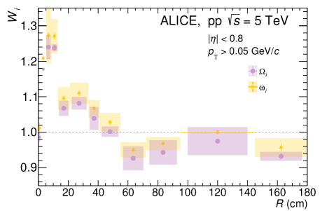
Figure 3: Distribution of the weights ${\Omega}_{i}$ and $\omega_{i}$ as a function of the radial position of the conversion point. Statistical uncertainties are given by the vertical bars, and systematic uncertainties are depicted by shaded areas, except for the first two intervals where only statistical uncertainties are quoted. Notice the zero $\omega_{i}$ systematic uncertainty in the calibration intervals (95 cm$<R<$ 145 cm), thus an horizontal line is drawn displaying the radial interval. The width in spatial direction of the uncertainty box for the $\Omega_{i}$ was shrunk for better visibility.

Table 3: Correction factors ${\Omega}_{i}$ for each radial interval used in this analysis, as well as the average value. Statistical, systematic, and total uncertainties are also given, except for the first two intervals where only statistical uncertainties are quoted.

$R$ interval	$R$ range (cm)	${\Omega}_{i}$	$\sigma_{\rm stat}$ %	$\sigma_{\rm sys}$ %	$\sigma_{\rm total}$ %
0	0–1.5	0.9859	1.2	-	-
1	1.5–5	1.177	0.42	-	-
2	5–8.5	1.240	0.36	2.7	2.8
3	8.5–13	1.238	0.42	0.77	0.9
4	13–21	1.067	0.34	2.0	2.1
5	21–33.5	1.081	0.25	1.7	1.7
6	33.5–41	1.039	0.35	3.1	3.1
7	41–55	1.001	0.30	1.5	1.5
8	55–72	0.926	0.35	3.7	3.7
9	72–95	0.943	0.19	3.7	3.7
10	95–145	0.975	0.62	4.1	4.1
11	145–180	0.932	0.89	1.4	1.6
average	5–180	1.04	0.312%	2.5%	2.5%

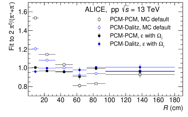
Figure 4: Zero-order polynomial fits to the ratio of neutral to charged pion transverse momentum distributions above 1 GeV/$c$ when the two photons (PCM-PCM, $\pi^{0}\rightarrow\gamma\gamma$) or one photon (PCM-Dalitz, $\pi^{0}\rightarrow e^{+}e^{-}\gamma$) are selected within the given radial interval. The open symbols are obtained with efficiency corrections using the default MC , while the full symbols are obtained when the $\Omega_{i}$ calibration factors are used to weight the efficiency (see Eq. 1).

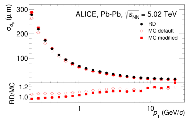
Figure 5: Top: Impact-parameter resolution of reconstructed charged particles requiring a hit in the first ITS pixel layer as a function of $p_{\rm T}$ in RD, default MC, and modified MC with the correction factors as given in Table 3. Bottom: Ratio of impact-parameter resolution to the one in the default MC (open circles) and modified MC (squares).

In order to further verify the correctness of the ${\Omega}_{i}$ values, $\pi^{0}$ measurements [9, 37, 38, 39] are carried out selecting photons in a given radial interval at a time, before and after applying the correction factors. The transverse momentum spectra of $\pi^{0}$ should not depend on the radial interval where the photons are reconstructed. $\pi^{0}$ transverse momentum spectra measured with two (or one) decay photons within one radial interval were analysed and compared to the spectra of charged pions [40], by fitting their ratios with a constant (see Fig. 4). The dispersion (rms) of the fit results is large when using the default MC. The fit results show clearly the same pattern as the calibration weights for the PCM-Dalitz analysis while for the PCM-PCM analysis the expected quadratic effect is observed. When using the ${\Omega}_{i}$, the rms reduces by almost a factor 10 when both photons are reconstructed with the PCM method, or by a factor $\sim$ 4 when only one PCM photon is used in the reconstruction, i.e., reconstructing either the Dalitz decay or reconstructing the second photon with a calorimeter. Furthermore, the ratio of the $\pi^{0}$ measurement in the complete radial range to the charged-pion measurement is in good agreement with the PYTHIA 8 expectations within one standard deviation.

Another observation corroborating the need for material budget correction factors is that the impact-parameter resolution of charged particles, i.e., the resolution of the reconstructed distance of closest approach of a track to the primary vertex, in RD is underestimated by the default MC. The small difference between data and MC of the particle composition plays a negligible effect, as most of the charged particles are charged pions. Fig. 5 shows the impact-parameter resolution of reconstructed charged particles with a hit in the first ITS pixel layer as a function of $p_{\rm T}$ for RD and for the default MC. The difference between RD and MC is usually corrected with an ad-hoc smearing of the track parameters in the MC. On the other hand, a modified MC simulation where the correction factors as given in Table 3 are used to scale the density of the detector materials reproduces the measured resolution for $p_{\rm T}$ $<$ 1 GeV/$c$, where the multiple scattering contribution is largest. This result confirms also that the assumption of attributing the correction factors to the material budget and not to the efficiency is correct. This demonstrates the importance of the material budget correction well beyond the reconstruction of photons with the conversion method.

6 Conclusions

Two data-driven calibration methods of the detector material description in ALICE, one based on the precise knowledge of the ALICE TPC gas and the other based on the approximate pion isospin symmetry and named $\omega_{i}$ and $\Omega_{i}$, were developed. A reduction of the systematic uncertainty of almost a factor of two is achieved in the material budget up to a radius $R=$ 180 cm corresponding approximately to the radial center of the TPC. Moreover, the differences between the description of the material distribution used for MC and the reality in the individual $R$ intervals are mitigated. This addresses the largest source of systematic uncertainty in analyses using photon conversions. It also reduces an important, and sometimes dominant, source of systematic uncertainty in analyses based on charged-particle tracking, in particular when secondary vertices are used. The upgraded ALICE experiment for Run 3 [41] will continue to use these two calibration methods. Moreover, to assist the $\omega_{i}$ method, two calibrated tungsten wires were inserted in the inner and the outer barrels of ITS2 [42]. These two methods are general in nature and could be applied to any experiment in a similar fashion.

Appendix A The ALICE Collaboration

S. Acharya  ¹²⁵, D. Adamová  ⁸⁶, A. Adler⁶⁹, G. Aglieri Rinella  ³², M. Agnello  ²⁹, N. Agrawal  ⁵⁰, Z. Ahammed  ¹³², S. Ahmad  ¹⁵, S.U. Ahn  ⁷⁰, I. Ahuja  ³⁷, A. Akindinov  ¹⁴⁰, M. Al-Turany  ⁹⁷, D. Aleksandrov  ¹⁴⁰, B. Alessandro  ⁵⁵, H.M. Alfanda  ⁶, R. Alfaro Molina  ⁶⁶, B. Ali  ¹⁵, A. Alici  ²⁵, N. Alizadehvandchali  ¹¹⁴, A. Alkin  ³², J. Alme  ²⁰, G. Alocco  ⁵¹, T. Alt  ⁶³, I. Altsybeev  ¹⁴⁰, M.N. Anaam  ⁶, C. Andrei  ⁴⁵, A. Andronic  ¹³⁵, V. Anguelov⁹⁴, F. Antinori  ⁵³, P. Antonioli  ⁵⁰, N. Apadula  ⁷⁴, L. Aphecetche  ¹⁰³, H. Appelshäuser  ⁶³, C. Arata  ⁷³, S. Arcelli  ²⁵, M. Aresti  ⁵¹, R. Arnaldi  ⁵⁵, J.G.M.C.A. Arneiro  ¹¹⁰, I.C. Arsene  ¹⁹, M. Arslandok  ¹³⁷, A. Augustinus  ³², R. Averbeck  ⁹⁷, M.D. Azmi  ¹⁵, A. Badalà  ⁵², J. Bae  ¹⁰⁴, Y.W. Baek  ⁴⁰, X. Bai  ¹¹⁸, R. Bailhache  ⁶³, Y. Bailung  ⁴⁷, A. Balbino  ²⁹, A. Baldisseri  ¹²⁸, B. Balis  ², D. Banerjee  ⁴, Z. Banoo  ⁹¹, R. Barbera  ²⁶, F. Barile  ³¹, L. Barioglio  ⁹⁵, M. Barlou⁷⁸, G.G. Barnaföldi  ¹³⁶, L.S. Barnby  ⁸⁵, V. Barret  ¹²⁵, L. Barreto  ¹¹⁰, C. Bartels  ¹¹⁷, K. Barth  ³², E. Bartsch  ⁶³, N. Bastid  ¹²⁵, S. Basu  ⁷⁵, G. Batigne  ¹⁰³, D. Battistini  ⁹⁵, B. Batyunya  ¹⁴¹, D. Bauri⁴⁶, J.L. Bazo Alba  ¹⁰¹, I.G. Bearden  ⁸³, C. Beattie  ¹³⁷, P. Becht  ⁹⁷, D. Behera  ⁴⁷, I. Belikov  ¹²⁷, A.D.C. Bell Hechavarria  ¹³⁵, F. Bellini  ²⁵, R. Bellwied  ¹¹⁴, S. Belokurova  ¹⁴⁰, G. Bencedi  ¹³⁶, S. Beole  ²⁴, A. Bercuci  ⁴⁵, Y. Berdnikov  ¹⁴⁰, A. Berdnikova  ⁹⁴, L. Bergmann  ⁹⁴, M.G. Besoiu  ⁶², L. Betev  ³², P.P. Bhaduri  ¹³², A. Bhasin  ⁹¹, M.A. Bhat  ⁴, B. Bhattacharjee  ⁴¹, L. Bianchi  ²⁴, N. Bianchi  ⁴⁸, J. Bielčík  ³⁵, J. Bielčíková  ⁸⁶, J. Biernat  ¹⁰⁷, A.P. Bigot  ¹²⁷, A. Bilandzic  ⁹⁵, G. Biro  ¹³⁶, S. Biswas  ⁴, N. Bize  ¹⁰³, J.T. Blair  ¹⁰⁸, D. Blau  ¹⁴⁰, M.B. Blidaru  ⁹⁷, N. Bluhme³⁸, C. Blume  ⁶³, G. Boca  ^21,54, F. Bock  ⁸⁷, T. Bodova  ²⁰, A. Bogdanov¹⁴⁰, S. Boi  ²², J. Bok  ⁵⁷, L. Boldizsár  ¹³⁶, M. Bombara  ³⁷, P.M. Bond  ³², G. Bonomi  ^131,54, H. Borel  ¹²⁸, A. Borissov  ¹⁴⁰, H. Bossi  ¹³⁷, E. Botta  ²⁴, Y.E.M. Bouziani  ⁶³, L. Bratrud  ⁶³, P. Braun-Munzinger  ⁹⁷, M. Bregant  ¹¹⁰, M. Broz  ³⁵, G.E. Bruno  ^96,31, M.D. Buckland  ²³, D. Budnikov¹⁴⁰, H. Buesching  ⁶³, S. Bufalino  ²⁹, P. Buhler  ¹⁰², Z. Buthelezi  ^67,121, A. Bylinkin  ²⁰, S.A. Bysiak¹⁰⁷, M. Cai  ⁶, H. Caines  ¹³⁷, A. Caliva  ²⁸, E. Calvo Villar  ¹⁰¹, J.M.M. Camacho  ¹⁰⁹, P. Camerini  ²³, F.D.M. Canedo  ¹¹⁰, M. Carabas  ¹²⁴, A.A. Carballo  ³², A.G.B. Carcamo  ⁹⁴, F. Carnesecchi  ³², R. Caron  ¹²⁶, L.A.D. Carvalho  ¹¹⁰, J. Castillo Castellanos  ¹²⁸, F. Catalano  ^32,24, C. Ceballos Sanchez  ¹⁴¹, I. Chakaberia  ⁷⁴, P. Chakraborty  ⁴⁶, S. Chandra  ¹³², S. Chapeland  ³², M. Chartier  ¹¹⁷, S. Chattopadhyay  ¹³², S. Chattopadhyay  ⁹⁹, T.G. Chavez  ⁴⁴, T. Cheng  ^97,6, C. Cheshkov  ¹²⁶, B. Cheynis  ¹²⁶, V. Chibante Barroso  ³², D.D. Chinellato  ¹¹¹, E.S. Chizzali  ⁹⁵, J. Cho  ⁵⁷, S. Cho  ⁵⁷, P. Chochula  ³², P. Christakoglou  ⁸⁴, C.H. Christensen  ⁸³, P. Christiansen  ⁷⁵, T. Chujo  ¹²³, M. Ciacco  ²⁹, C. Cicalo  ⁵¹, F. Cindolo  ⁵⁰, M.R. Ciupek⁹⁷, G. Clai^II,50, F. Colamaria  ⁴⁹, J.S. Colburn¹⁰⁰, D. Colella  ^96,31, M. Colocci  ²⁵, G. Conesa Balbastre  ⁷³, Z. Conesa del Valle  ⁷², G. Contin  ²³, J.G. Contreras  ³⁵, M.L. Coquet  ¹²⁸, T.M. Cormier^I,87, P. Cortese  ^130,55, M.R. Cosentino  ¹¹², F. Costa  ³², S. Costanza  ^21,54, C. Cot  ⁷², J. Crkovská  ⁹⁴, P. Crochet  ¹²⁵, R. Cruz-Torres  ⁷⁴, P. Cui  ⁶, A. Dainese  ⁵³, M.C. Danisch  ⁹⁴, A. Danu  ⁶², P. Das  ⁸⁰, P. Das  ⁴, S. Das  ⁴, A.R. Dash  ¹³⁵, S. Dash  ⁴⁶, A. De Caro  ²⁸, G. de Cataldo  ⁴⁹, J. de Cuveland³⁸, A. De Falco  ²², D. De Gruttola  ²⁸, N. De Marco  ⁵⁵, C. De Martin  ²³, S. De Pasquale  ²⁸, R. Deb¹³¹, S. Deb  ⁴⁷, K.R. Deja¹³³, R. Del Grande  ⁹⁵, L. Dello Stritto  ²⁸, W. Deng  ⁶, P. Dhankher  ¹⁸, D. Di Bari  ³¹, A. Di Mauro  ³², B. Diab  ¹²⁸, R.A. Diaz  ^141,7, T. Dietel  ¹¹³, Y. Ding  ⁶, R. Divià  ³², D.U. Dixit  ¹⁸, Ø. Djuvsland²⁰, U. Dmitrieva  ¹⁴⁰, A. Dobrin  ⁶², B. Dönigus  ⁶³, J.M. Dubinski¹³³, A. Dubla  ⁹⁷, S. Dudi  ⁹⁰, P. Dupieux  ¹²⁵, M. Durkac¹⁰⁶, N. Dzalaiova¹², T.M. Eder  ¹³⁵, R.J. Ehlers  ⁷⁴, F. Eisenhut  ⁶³, D. Elia  ⁴⁹, B. Erazmus  ¹⁰³, F. Ercolessi  ²⁵, F. Erhardt  ⁸⁹, M.R. Ersdal²⁰, B. Espagnon  ⁷², G. Eulisse  ³², D. Evans  ¹⁰⁰, S. Evdokimov  ¹⁴⁰, L. Fabbietti  ⁹⁵, M. Faggin  ²⁷, J. Faivre  ⁷³, F. Fan  ⁶, W. Fan  ⁷⁴, A. Fantoni  ⁴⁸, M. Fasel  ⁸⁷, P. Fecchio²⁹, A. Feliciello  ⁵⁵, G. Feofilov  ¹⁴⁰, A. Fernández Téllez  ⁴⁴, L. Ferrandi  ¹¹⁰, M.B. Ferrer  ³², A. Ferrero  ¹²⁸, C. Ferrero  ⁵⁵, A. Ferretti  ²⁴, V.J.G. Feuillard  ⁹⁴, V. Filova³⁵, D. Finogeev  ¹⁴⁰, F.M. Fionda  ⁵¹, F. Flor  ¹¹⁴, A.N. Flores  ¹⁰⁸, S. Foertsch  ⁶⁷, I. Fokin  ⁹⁴, S. Fokin  ¹⁴⁰, E. Fragiacomo  ⁵⁶, E. Frajna  ¹³⁶, U. Fuchs  ³², N. Funicello  ²⁸, C. Furget  ⁷³, A. Furs  ¹⁴⁰, T. Fusayasu  ⁹⁸, J.J. Gaardhøje  ⁸³, M. Gagliardi  ²⁴, A.M. Gago  ¹⁰¹, C.D. Galvan  ¹⁰⁹, D.R. Gangadharan  ¹¹⁴, P. Ganoti  ⁷⁸, C. Garabatos  ⁹⁷, J.R.A. Garcia  ⁴⁴, E. Garcia-Solis  ⁹, C. Gargiulo  ³², A. Garibli⁸¹, K. Garner¹³⁵, P. Gasik  ⁹⁷, A. Gautam  ¹¹⁶, M.B. Gay Ducati  ⁶⁵, M. Germain  ¹⁰³, A. Ghimouz¹²³, C. Ghosh¹³², M. Giacalone  ^50,25, P. Giubellino  ^97,55, P. Giubilato  ²⁷, A.M.C. Glaenzer  ¹²⁸, P. Glässel  ⁹⁴, E. Glimos¹²⁰, D.J.Q. Goh⁷⁶, V. Gonzalez  ¹³⁴, S. Gorbunov³⁸, M. Gorgon  ², K. Goswami  ⁴⁷, S. Gotovac³³, V. Grabski  ⁶⁶, L.K. Graczykowski  ¹³³, E. Grecka  ⁸⁶, A. Grelli  ⁵⁸, C. Grigoras  ³², V. Grigoriev  ¹⁴⁰, S. Grigoryan  ^141,1, F. Grosa  ³², J.F. Grosse-Oetringhaus  ³², R. Grosso  ⁹⁷, D. Grund  ³⁵, G.G. Guardiano  ¹¹¹, R. Guernane  ⁷³, M. Guilbaud  ¹⁰³, K. Gulbrandsen  ⁸³, T. Gundem  ⁶³, T. Gunji  ¹²², W. Guo  ⁶, A. Gupta  ⁹¹, R. Gupta  ⁹¹, R. Gupta  ⁴⁷, S.P. Guzman  ⁴⁴, K. Gwizdziel  ¹³³, L. Gyulai  ¹³⁶, M.K. Habib⁹⁷, C. Hadjidakis  ⁷², F.U. Haider  ⁹¹, H. Hamagaki  ⁷⁶, A. Hamdi  ⁷⁴, M. Hamid⁶, Y. Han  ¹³⁸, B.G. Hanley  ¹³⁴, R. Hannigan  ¹⁰⁸, J. Hansen  ⁷⁵, M.R. Haque  ¹³³, J.W. Harris  ¹³⁷, A. Harton  ⁹, H. Hassan  ⁸⁷, D. Hatzifotiadou  ⁵⁰, P. Hauer  ⁴², L.B. Havener  ¹³⁷, S.T. Heckel  ⁹⁵, E. Hellbär  ⁹⁷, H. Helstrup  ³⁴, M. Hemmer  ⁶³, T. Herman  ³⁵, G. Herrera Corral  ⁸, F. Herrmann¹³⁵, S. Herrmann  ¹²⁶, K.F. Hetland  ³⁴, B. Heybeck  ⁶³, H. Hillemanns  ³², B. Hippolyte  ¹²⁷, F.W. Hoffmann  ⁶⁹, B. Hofman  ⁵⁸, B. Hohlweger  ⁸⁴, G.H. Hong  ¹³⁸, M. Horst  ⁹⁵, A. Horzyk  ², Y. Hou  ⁶, P. Hristov  ³², C. Hughes  ¹²⁰, P. Huhn⁶³, L.M. Huhta  ¹¹⁵, T.J. Humanic  ⁸⁸, L.A. Husova  ¹³⁵, A. Hutson  ¹¹⁴, R. Ilkaev¹⁴⁰, H. Ilyas  ¹³, M. Inaba  ¹²³, G.M. Innocenti  ³², M. Ippolitov  ¹⁴⁰, A. Isakov  ⁸⁶, T. Isidori  ¹¹⁶, M.S. Islam  ⁹⁹, M. Ivanov  ⁹⁷, M. Ivanov¹², V. Ivanov  ¹⁴⁰, K.E. Iversen  ⁷⁵, M. Jablonski  ², B. Jacak⁷⁴, N. Jacazio  ²⁵, P.M. Jacobs  ⁷⁴, S. Jadlovska¹⁰⁶, J. Jadlovsky¹⁰⁶, S. Jaelani  ⁸², C. Jahnke¹¹¹, M.J. Jakubowska  ¹³³, M.A. Janik  ¹³³, T. Janson⁶⁹, M. Jercic⁸⁹, S. Ji  ¹⁶, S. Jia  ¹⁰, A.A.P. Jimenez  ⁶⁴, F. Jonas  ⁸⁷, J.M. Jowett   ^32,97, J. Jung  ⁶³, M. Jung  ⁶³, A. Junique  ³², A. Jusko  ¹⁰⁰, M.J. Kabus  ^32,133, J. Kaewjai¹⁰⁵, P. Kalinak  ⁵⁹, A.S. Kalteyer  ⁹⁷, A. Kalweit  ³², V. Kaplin  ¹⁴⁰, A. Karasu Uysal  ⁷¹, D. Karatovic  ⁸⁹, O. Karavichev  ¹⁴⁰, T. Karavicheva  ¹⁴⁰, P. Karczmarczyk  ¹³³, E. Karpechev  ¹⁴⁰, U. Kebschull  ⁶⁹, R. Keidel  ¹³⁹, D.L.D. Keijdener⁵⁸, M. Keil  ³², B. Ketzer  ⁴², S.S. Khade  ⁴⁷, A.M. Khan  ⁶, S. Khan  ¹⁵, A. Khanzadeev  ¹⁴⁰, Y. Kharlov  ¹⁴⁰, A. Khatun  ¹¹⁶, A. Khuntia  ¹⁰⁷, M.B. Kidson¹¹³, B. Kileng  ³⁴, B. Kim  ¹⁰⁴, C. Kim  ¹⁶, D.J. Kim  ¹¹⁵, E.J. Kim  ⁶⁸, J. Kim  ¹³⁸, J.S. Kim  ⁴⁰, J. Kim  ⁵⁷, J. Kim  ⁶⁸, M. Kim  ¹⁸, S. Kim  ¹⁷, T. Kim  ¹³⁸, K. Kimura  ⁹², S. Kirsch  ⁶³, I. Kisel  ³⁸, S. Kiselev  ¹⁴⁰, A. Kisiel  ¹³³, J.P. Kitowski  ², J.L. Klay  ⁵, J. Klein  ³², S. Klein  ⁷⁴, C. Klein-Bösing  ¹³⁵, M. Kleiner  ⁶³, T. Klemenz  ⁹⁵, A. Kluge  ³², A.G. Knospe  ¹¹⁴, C. Kobdaj  ¹⁰⁵, T. Kollegger⁹⁷, A. Kondratyev  ¹⁴¹, N. Kondratyeva  ¹⁴⁰, E. Kondratyuk  ¹⁴⁰, J. Konig  ⁶³, S.A. Konigstorfer  ⁹⁵, P.J. Konopka  ³², G. Kornakov  ¹³³, S.D. Koryciak  ², A. Kotliarov  ⁸⁶, V. Kovalenko  ¹⁴⁰, M. Kowalski  ¹⁰⁷, V. Kozhuharov  ³⁶, I. Králik  ⁵⁹, A. Kravčáková  ³⁷, L. Krcal  ^32,38, M. Krivda  ^100,59, F. Krizek  ⁸⁶, K. Krizkova Gajdosova  ³², M. Kroesen  ⁹⁴, M. Krüger  ⁶³, D.M. Krupova  ³⁵, E. Kryshen  ¹⁴⁰, V. Kučera  ⁵⁷, C. Kuhn  ¹²⁷, P.G. Kuijer  ⁸⁴, T. Kumaoka¹²³, D. Kumar¹³², L. Kumar  ⁹⁰, N. Kumar⁹⁰, S. Kumar  ³¹, S. Kundu  ³², P. Kurashvili  ⁷⁹, A. Kurepin  ¹⁴⁰, A.B. Kurepin  ¹⁴⁰, A. Kuryakin  ¹⁴⁰, S. Kushpil  ⁸⁶, J. Kvapil  ¹⁰⁰, M.J. Kweon  ⁵⁷, Y. Kwon  ¹³⁸, S.L. La Pointe  ³⁸, P. La Rocca  ²⁶, A. Lakrathok¹⁰⁵, M. Lamanna  ³², R. Langoy  ¹¹⁹, P. Larionov  ³², E. Laudi  ³², L. Lautner  ^32,95, R. Lavicka  ¹⁰², R. Lea  ^131,54, L. Leardini⁹⁴, H. Lee  ¹⁰⁴, I. Legrand  ⁴⁵, G. Legras  ¹³⁵, J. Lehrbach  ³⁸, T.M. Lelek², R.C. Lemmon  ⁸⁵, I. León Monzón  ¹⁰⁹, M.M. Lesch  ⁹⁵, E.D. Lesser  ¹⁸, P. Lévai  ¹³⁶, X. Li¹⁰, X.L. Li⁶, J. Lien  ¹¹⁹, R. Lietava  ¹⁰⁰, I. Likmeta  ¹¹⁴, B. Lim  ²⁴, S.H. Lim  ¹⁶, V. Lindenstruth  ³⁸, A. Lindner⁴⁵, C. Lippmann  ⁹⁷, A. Liu  ¹⁸, D.H. Liu  ⁶, J. Liu  ¹¹⁷, G.S.S. Liveraro  ¹¹¹, I.M. Lofnes  ²⁰, C. Loizides  ⁸⁷, S. Lokos  ¹⁰⁷, J. Lomker  ⁵⁸, P. Loncar  ³³, J.A. Lopez  ⁹⁴, X. Lopez  ¹²⁵, E. López Torres  ⁷, P. Lu  ^97,118, J.R. Luhder  ¹³⁵, M. Lunardon  ²⁷, G. Luparello  ⁵⁶, Y.G. Ma  ³⁹, M. Mager  ³², A. Maire  ¹²⁷, M.V. Makariev  ³⁶, M. Malaev  ¹⁴⁰, G. Malfattore  ²⁵, N.M. Malik  ⁹¹, Q.W. Malik¹⁹, S.K. Malik  ⁹¹, L. Malinina  ^V,141, D. Mallick  ⁸⁰, N. Mallick  ⁴⁷, G. Mandaglio  ^30,52, S.K. Mandal  ⁷⁹, V. Manko  ¹⁴⁰, F. Manso  ¹²⁵, V. Manzari  ⁴⁹, Y. Mao  ⁶, R.W. Marcjan  ², G.V. Margagliotti  ²³, A. Margotti  ⁵⁰, A. Marín  ⁹⁷, C. Markert  ¹⁰⁸, P. Martinengo  ³², M.I. Martínez  ⁴⁴, G. Martínez García  ¹⁰³, M.P.P. Martins  ¹¹⁰, S. Masciocchi  ⁹⁷, M. Masera  ²⁴, A. Masoni  ⁵¹, L. Massacrier  ⁷², A. Mastroserio  ^129,49, O. Matonoha  ⁷⁵, S. Mattiazzo  ²⁷, P.F.T. Matuoka¹¹⁰, A. Matyja  ¹⁰⁷, C. Mayer  ¹⁰⁷, A.L. Mazuecos  ³², F. Mazzaschi  ²⁴, M. Mazzilli  ³², J.E. Mdhluli  ¹²¹, A.F. Mechler⁶³, Y. Melikyan  ^43,140, A. Menchaca-Rocha  ⁶⁶, E. Meninno  ^102,28, A.S. Menon  ¹¹⁴, M. Meres  ¹², S. Mhlanga^113,67, Y. Miake¹²³, L. Micheletti  ³², L.C. Migliorin¹²⁶, D.L. Mihaylov  ⁹⁵, K. Mikhaylov  ^141,140, A.N. Mishra  ¹³⁶, D. Miśkowiec  ⁹⁷, A. Modak  ⁴, A.P. Mohanty  ⁵⁸, B. Mohanty  ⁸⁰, M. Mohisin Khan  ^III,15, M.A. Molander  ⁴³, Z. Moravcova  ⁸³, C. Mordasini  ⁹⁵, D.A. Moreira De Godoy  ¹³⁵, I. Morozov  ¹⁴⁰, A. Morsch  ³², T. Mrnjavac  ³², V. Muccifora  ⁴⁸, S. Muhuri  ¹³², J.D. Mulligan  ⁷⁴, A. Mulliri²², M.G. Munhoz  ¹¹⁰, R.H. Munzer  ⁶³, H. Murakami  ¹²², S. Murray  ¹¹³, L. Musa  ³², J. Musinsky  ⁵⁹, J.W. Myrcha  ¹³³, B. Naik  ¹²¹, A.I. Nambrath  ¹⁸, B.K. Nandi⁴⁶, R. Nania  ⁵⁰, E. Nappi  ⁴⁹, A.F. Nassirpour  ^17,75, A. Nath  ⁹⁴, C. Nattrass  ¹²⁰, M.N. Naydenov  ³⁶, A. Neagu¹⁹, A. Negru¹²⁴, L. Nellen  ⁶⁴, G. Neskovic  ³⁸, B.S. Nielsen  ⁸³, E.G. Nielsen  ⁸³, S. Nikolaev  ¹⁴⁰, S. Nikulin  ¹⁴⁰, V. Nikulin  ¹⁴⁰, F. Noferini  ⁵⁰, S. Noh  ¹¹, P. Nomokonov  ¹⁴¹, J. Norman  ¹¹⁷, N. Novitzky  ¹²³, P. Nowakowski  ¹³³, A. Nyanin  ¹⁴⁰, J. Nystrand  ²⁰, M. Ogino  ⁷⁶, A. Ohlson  ⁷⁵, V.A. Okorokov  ¹⁴⁰, J. Oleniacz  ¹³³, A.C. Oliveira Da Silva  ¹²⁰, M.H. Oliver  ¹³⁷, A. Onnerstad  ¹¹⁵, C. Oppedisano  ⁵⁵, A. Ortiz Velasquez  ⁶⁴, J. Otwinowski  ¹⁰⁷, M. Oya⁹², K. Oyama  ⁷⁶, Y. Pachmayer  ⁹⁴, S. Padhan  ⁴⁶, D. Pagano  ^131,54, G. Paić  ⁶⁴, A. Palasciano  ⁴⁹, S. Panebianco  ¹²⁸, H. Park  ¹²³, H. Park  ¹⁰⁴, J. Park  ⁵⁷, J.E. Parkkila  ³², R.N. Patra⁹¹, B. Paul  ²², H. Pei  ⁶, T. Peitzmann  ⁵⁸, X. Peng  ⁶, M. Pennisi  ²⁴, D. Peresunko  ¹⁴⁰, G.M. Perez  ⁷, S. Perrin  ¹²⁸, Y. Pestov¹⁴⁰, V. Petrov  ¹⁴⁰, M. Petrovici  ⁴⁵, R.P. Pezzi  ^103,65, S. Piano  ⁵⁶, M. Pikna  ¹², P. Pillot  ¹⁰³, O. Pinazza  ^50,32, L. Pinsky¹¹⁴, C. Pinto  ⁹⁵, S. Pisano  ⁴⁸, M. Płoskoń  ⁷⁴, M. Planinic⁸⁹, F. Pliquett⁶³, M.G. Poghosyan  ⁸⁷, B. Polichtchouk  ¹⁴⁰, S. Politano  ²⁹, N. Poljak  ⁸⁹, A. Pop  ⁴⁵, S. Porteboeuf-Houssais  ¹²⁵, V. Pozdniakov  ¹⁴¹, I.Y. Pozos  ⁴⁴, K.K. Pradhan  ⁴⁷, S.K. Prasad  ⁴, S. Prasad  ⁴⁷, R. Preghenella  ⁵⁰, F. Prino  ⁵⁵, C.A. Pruneau  ¹³⁴, I. Pshenichnov  ¹⁴⁰, M. Puccio  ³², S. Pucillo  ²⁴, Z. Pugelova¹⁰⁶, S. Qiu  ⁸⁴, L. Quaglia  ²⁴, R.E. Quishpe¹¹⁴, S. Ragoni  ¹⁴, A. Rakotozafindrabe  ¹²⁸, L. Ramello  ^130,55, F. Rami  ¹²⁷, S.A.R. Ramirez  ⁴⁴, T.A. Rancien⁷³, M. Rasa  ²⁶, S.S. Räsänen  ⁴³, R. Rath  ⁵⁰, M.P. Rauch  ²⁰, I. Ravasenga  ⁸⁴, K.F. Read  ^87,120, C. Reckziegel  ¹¹², A.R. Redelbach  ³⁸, K. Redlich  ^IV,79, C.A. Reetz  ⁹⁷, A. Rehman²⁰, F. Reidt  ³², H.A. Reme-Ness  ³⁴, Z. Rescakova³⁷, K. Reygers  ⁹⁴, A. Riabov  ¹⁴⁰, V. Riabov  ¹⁴⁰, R. Ricci  ²⁸, M. Richter¹⁹, A.A. Riedel  ⁹⁵, W. Riegler  ³², C. Ristea  ⁶², M.V. Rodriguez  ³², M. Rodríguez Cahuantzi  ⁴⁴, K. Røed  ¹⁹, R. Rogalev  ¹⁴⁰, E. Rogochaya  ¹⁴¹, T.S. Rogoschinski  ⁶³, D. Rohr  ³², D. Röhrich  ²⁰, P.F. Rojas⁴⁴, S. Rojas Torres  ³⁵, P.S. Rokita  ¹³³, G. Romanenko  ¹⁴¹, F. Ronchetti  ⁴⁸, A. Rosano  ^30,52, E.D. Rosas⁶⁴, K. Roslon  ¹³³, A. Rossi  ⁵³, A. Roy  ⁴⁷, S. Roy⁴⁶, N. Rubini  ²⁵, O.V. Rueda  ¹¹⁴, D. Ruggiano  ¹³³, R. Rui  ²³, P.G. Russek  ², R. Russo  ⁸⁴, A. Rustamov  ⁸¹, E. Ryabinkin  ¹⁴⁰, Y. Ryabov  ¹⁴⁰, A. Rybicki  ¹⁰⁷, H. Rytkonen  ¹¹⁵, J. Ryu  ¹⁶, W. Rzesa  ¹³³, O.A.M. Saarimaki  ⁴³, R. Sadek  ¹⁰³, S. Sadhu  ³¹, S. Sadovsky  ¹⁴⁰, J. Saetre  ²⁰, K. Šafařík  ³⁵, P. Saha⁴¹, S.K. Saha  ⁴, S. Saha  ⁸⁰, B. Sahoo  ⁴⁶, B. Sahoo  ⁴⁷, R. Sahoo  ⁴⁷, S. Sahoo⁶⁰, D. Sahu  ⁴⁷, P.K. Sahu  ⁶⁰, J. Saini  ¹³², K. Sajdakova³⁷, S. Sakai  ¹²³, M.P. Salvan  ⁹⁷, S. Sambyal  ⁹¹, I. Sanna  ^32,95, T.B. Saramela¹¹⁰, D. Sarkar  ¹³⁴, N. Sarkar¹³², P. Sarma⁴¹, V. Sarritzu  ²², V.M. Sarti  ⁹⁵, M.H.P. Sas  ¹³⁷, J. Schambach  ⁸⁷, H.S. Scheid  ⁶³, C. Schiaua  ⁴⁵, R. Schicker  ⁹⁴, A. Schmah⁹⁴, C. Schmidt  ⁹⁷, H.R. Schmidt⁹³, M.O. Schmidt  ³², M. Schmidt⁹³, N.V. Schmidt  ⁸⁷, A.R. Schmier  ¹²⁰, R. Schotter  ¹²⁷, A. Schröter  ³⁸, J. Schukraft  ³², K. Schwarz⁹⁷, K. Schweda  ⁹⁷, G. Scioli  ²⁵, E. Scomparin  ⁵⁵, J.E. Seger  ¹⁴, Y. Sekiguchi¹²², D. Sekihata  ¹²², I. Selyuzhenkov  ⁹⁷, S. Senyukov  ¹²⁷, J.J. Seo  ⁵⁷, D. Serebryakov  ¹⁴⁰, L. Šerkšnytė  ⁹⁵, A. Sevcenco  ⁶², T.J. Shaba  ⁶⁷, A. Shabetai  ¹⁰³, R. Shahoyan³², A. Shangaraev  ¹⁴⁰, A. Sharma⁹⁰, B. Sharma  ⁹¹, D. Sharma  ⁴⁶, H. Sharma  ^53,107, M. Sharma  ⁹¹, S. Sharma  ⁷⁶, S. Sharma  ⁹¹, U. Sharma  ⁹¹, A. Shatat  ⁷², O. Sheibani¹¹⁴, K. Shigaki  ⁹², M. Shimomura⁷⁷, J. Shin¹¹, S. Shirinkin  ¹⁴⁰, Q. Shou  ³⁹, Y. Sibiriak  ¹⁴⁰, S. Siddhanta  ⁵¹, T. Siemiarczuk  ⁷⁹, T.F. Silva  ¹¹⁰, D. Silvermyr  ⁷⁵, T. Simantathammakul¹⁰⁵, R. Simeonov  ³⁶, B. Singh⁹¹, B. Singh  ⁹⁵, K. Singh  ⁴⁷, R. Singh  ⁸⁰, R. Singh  ⁹¹, R. Singh  ⁴⁷, S. Singh  ¹⁵, V.K. Singh  ¹³², V. Singhal  ¹³², T. Sinha  ⁹⁹, B. Sitar  ¹², M. Sitta  ^130,55, T.B. Skaali¹⁹, G. Skorodumovs  ⁹⁴, M. Slupecki  ⁴³, N. Smirnov  ¹³⁷, R.J.M. Snellings  ⁵⁸, E.H. Solheim  ¹⁹, J. Song  ¹¹⁴, A. Songmoolnak¹⁰⁵, C. Sonnabend  ^32,97, F. Soramel  ²⁷, A.B. Soto-hernandez⁸⁸, R. Spijkers  ⁸⁴, I. Sputowska  ¹⁰⁷, J. Staa  ⁷⁵, J. Stachel  ⁹⁴, I. Stan  ⁶², P.J. Steffanic  ¹²⁰, S.F. Stiefelmaier  ⁹⁴, D. Stocco  ¹⁰³, I. Storehaug  ¹⁹, P. Stratmann  ¹³⁵, S. Strazzi  ²⁵, C.P. Stylianidis⁸⁴, A.A.P. Suaide  ¹¹⁰, C. Suire  ⁷², M. Sukhanov  ¹⁴⁰, M. Suljic  ³², R. Sultanov  ¹⁴⁰, V. Sumberia  ⁹¹, S. Sumowidagdo  ⁸², S. Swain⁶⁰, I. Szarka  ¹², M. Szymkowski¹³³, S.F. Taghavi  ⁹⁵, G. Taillepied  ⁹⁷, J. Takahashi  ¹¹¹, G.J. Tambave  ⁸⁰, S. Tang  ⁶, Z. Tang  ¹¹⁸, J.D. Tapia Takaki  ¹¹⁶, N. Tapus¹²⁴, M.G. Tarzila⁴⁵, G.F. Tassielli  ³¹, A. Tauro  ³², G. Tejeda Muñoz  ⁴⁴, A. Telesca  ³², L. Terlizzi  ²⁴, C. Terrevoli  ¹¹⁴, S. Thakur  ⁴, D. Thomas  ¹⁰⁸, A. Tikhonov  ¹⁴⁰, A.R. Timmins  ¹¹⁴, M. Tkacik¹⁰⁶, T. Tkacik  ¹⁰⁶, A. Toia  ⁶³, R. Tokumoto⁹², N. Topilskaya  ¹⁴⁰, M. Toppi  ⁴⁸, T. Tork  ⁷², A.G. Torres Ramos  ³¹, A. Trifiró  ^30,52, A.S. Triolo  ^32,30,52, S. Tripathy  ⁵⁰, T. Tripathy  ⁴⁶, S. Trogolo  ³², V. Trubnikov  ³, W.H. Trzaska  ¹¹⁵, T.P. Trzcinski  ¹³³, A. Tumkin¹⁴⁰, R. Turrisi  ⁵³, T.S. Tveter  ¹⁹, K. Ullaland  ²⁰, B. Ulukutlu  ⁹⁵, A. Uras  ¹²⁶, M. Urioni  ^54,131, G.L. Usai  ²², M. Vala³⁷, N. Valle  ²¹, L.V.R. van Doremalen⁵⁸, M. van Leeuwen  ⁸⁴, C.A. van Veen  ⁹⁴, R.J.G. van Weelden  ⁸⁴, P. Vande Vyvre  ³², D. Varga  ¹³⁶, Z. Varga  ¹³⁶, M. Vasileiou  ⁷⁸, A. Vasiliev  ¹⁴⁰, O. Vázquez Doce  ⁴⁸, V. Vechernin  ¹⁴⁰, E. Vercellin  ²⁴, S. Vergara Limón⁴⁴, L. Vermunt  ⁹⁷, R. Vértesi  ¹³⁶, M. Verweij  ⁵⁸, L. Vickovic³³, Z. Vilakazi¹²¹, O. Villalobos Baillie  ¹⁰⁰, A. Villani  ²³, G. Vino  ⁴⁹, A. Vinogradov  ¹⁴⁰, T. Virgili  ²⁸, M.M.O. Virta  ¹¹⁵, V. Vislavicius⁷⁵, A. Vodopyanov  ¹⁴¹, B. Volkel  ³², M.A. Völkl  ⁹⁴, K. Voloshin¹⁴⁰, S.A. Voloshin  ¹³⁴, G. Volpe  ³¹, B. von Haller  ³², I. Vorobyev  ⁹⁵, N. Vozniuk  ¹⁴⁰, J. Vrláková  ³⁷, J. Wan³⁹, C. Wang  ³⁹, D. Wang³⁹, Y. Wang  ³⁹, A. Wegrzynek  ³², F.T. Weiglhofer³⁸, S.C. Wenzel  ³², J.P. Wessels  ¹³⁵, S.L. Weyhmiller  ¹³⁷, J. Wiechula  ⁶³, J. Wikne  ¹⁹, G. Wilk  ⁷⁹, J. Wilkinson  ⁹⁷, G.A. Willems  ¹³⁵, B. Windelband⁹⁴, M. Winn  ¹²⁸, J.R. Wright  ¹⁰⁸, W. Wu³⁹, Y. Wu  ¹¹⁸, R. Xu  ⁶, A. Yadav  ⁴², A.K. Yadav  ¹³², S. Yalcin  ⁷¹, Y. Yamaguchi⁹², S. Yang²⁰, S. Yano  ⁹², Z. Yin  ⁶, I.-K. Yoo  ¹⁶, J.H. Yoon  ⁵⁷, H. Yu¹¹, S. Yuan²⁰, A. Yuncu  ⁹⁴, V. Zaccolo  ²³, C. Zampolli  ³², F. Zanone  ⁹⁴, N. Zardoshti  ³², A. Zarochentsev  ¹⁴⁰, P. Závada  ⁶¹, N. Zaviyalov¹⁴⁰, M. Zhalov  ¹⁴⁰, B. Zhang  ⁶, L. Zhang  ³⁹, S. Zhang  ³⁹, X. Zhang  ⁶, Y. Zhang¹¹⁸, Z. Zhang  ⁶, M. Zhao  ¹⁰, V. Zherebchevskii  ¹⁴⁰, Y. Zhi¹⁰, D. Zhou  ⁶, Y. Zhou  ⁸³, J. Zhu  ^97,6, Y. Zhu⁶, S.C. Zugravel  ⁵⁵, N. Zurlo  ^131,54

Affiliation Notes

^I Deceased
^II Also at: Italian National Agency for New Technologies, Energy and Sustainable Economic Development (ENEA), Bologna, Italy
^III Also at: Department of Applied Physics, Aligarh Muslim University, Aligarh, India
^IV Also at: Institute of Theoretical Physics, University of Wroclaw, Poland
^V Also at: An institution covered by a cooperation agreement with CERN

Collaboration Institutes

¹ A.I. Alikhanyan National Science Laboratory (Yerevan Physics Institute) Foundation, Yerevan, Armenia
² AGH University of Science and Technology, Cracow, Poland
³ Bogolyubov Institute for Theoretical Physics, National Academy of Sciences of Ukraine, Kiev, Ukraine
⁴ Bose Institute, Department of Physics and Centre for Astroparticle Physics and Space Science (CAPSS), Kolkata, India
⁵ California Polytechnic State University, San Luis Obispo, California, United States
⁶ Central China Normal University, Wuhan, China
⁷ Centro de Aplicaciones Tecnológicas y Desarrollo Nuclear (CEADEN), Havana, Cuba
⁸ Centro de Investigación y de Estudios Avanzados (CINVESTAV), Mexico City and Mérida, Mexico
⁹ Chicago State University, Chicago, Illinois, United States
¹⁰ China Institute of Atomic Energy, Beijing, China
¹¹ Chungbuk National University, Cheongju, Republic of Korea
¹² Comenius University Bratislava, Faculty of Mathematics, Physics and Informatics, Bratislava, Slovak Republic
¹³ COMSATS University Islamabad, Islamabad, Pakistan
¹⁴ Creighton University, Omaha, Nebraska, United States
¹⁵ Department of Physics, Aligarh Muslim University, Aligarh, India
¹⁶ Department of Physics, Pusan National University, Pusan, Republic of Korea
¹⁷ Department of Physics, Sejong University, Seoul, Republic of Korea
¹⁸ Department of Physics, University of California, Berkeley, California, United States
¹⁹ Department of Physics, University of Oslo, Oslo, Norway
²⁰ Department of Physics and Technology, University of Bergen, Bergen, Norway
²¹ Dipartimento di Fisica, Università di Pavia, Pavia, Italy
²² Dipartimento di Fisica dell’Università and Sezione INFN, Cagliari, Italy
²³ Dipartimento di Fisica dell’Università and Sezione INFN, Trieste, Italy
²⁴ Dipartimento di Fisica dell’Università and Sezione INFN, Turin, Italy
²⁵ Dipartimento di Fisica e Astronomia dell’Università and Sezione INFN, Bologna, Italy
²⁶ Dipartimento di Fisica e Astronomia dell’Università and Sezione INFN, Catania, Italy
²⁷ Dipartimento di Fisica e Astronomia dell’Università and Sezione INFN, Padova, Italy
²⁸ Dipartimento di Fisica ‘E.R. Caianiello’ dell’Università and Gruppo Collegato INFN, Salerno, Italy
²⁹ Dipartimento DISAT del Politecnico and Sezione INFN, Turin, Italy
³⁰ Dipartimento di Scienze MIFT, Università di Messina, Messina, Italy
³¹ Dipartimento Interateneo di Fisica ‘M. Merlin’ and Sezione INFN, Bari, Italy
³² European Organization for Nuclear Research (CERN), Geneva, Switzerland
³³ Faculty of Electrical Engineering, Mechanical Engineering and Naval Architecture, University of Split, Split, Croatia
³⁴ Faculty of Engineering and Science, Western Norway University of Applied Sciences, Bergen, Norway
³⁵ Faculty of Nuclear Sciences and Physical Engineering, Czech Technical University in Prague, Prague, Czech Republic
³⁶ Faculty of Physics, Sofia University, Sofia, Bulgaria
³⁷ Faculty of Science, P.J. Šafárik University, Košice, Slovak Republic
³⁸ Frankfurt Institute for Advanced Studies, Johann Wolfgang Goethe-Universität Frankfurt, Frankfurt, Germany
³⁹ Fudan University, Shanghai, China
⁴⁰ Gangneung-Wonju National University, Gangneung, Republic of Korea
⁴¹ Gauhati University, Department of Physics, Guwahati, India
⁴² Helmholtz-Institut für Strahlen- und Kernphysik, Rheinische Friedrich-Wilhelms-Universität Bonn, Bonn, Germany
⁴³ Helsinki Institute of Physics (HIP), Helsinki, Finland
⁴⁴ High Energy Physics Group, Universidad Autónoma de Puebla, Puebla, Mexico
⁴⁵ Horia Hulubei National Institute of Physics and Nuclear Engineering, Bucharest, Romania
⁴⁶ Indian Institute of Technology Bombay (IIT), Mumbai, India
⁴⁷ Indian Institute of Technology Indore, Indore, India
⁴⁸ INFN, Laboratori Nazionali di Frascati, Frascati, Italy
⁴⁹ INFN, Sezione di Bari, Bari, Italy
⁵⁰ INFN, Sezione di Bologna, Bologna, Italy
⁵¹ INFN, Sezione di Cagliari, Cagliari, Italy
⁵² INFN, Sezione di Catania, Catania, Italy
⁵³ INFN, Sezione di Padova, Padova, Italy
⁵⁴ INFN, Sezione di Pavia, Pavia, Italy
⁵⁵ INFN, Sezione di Torino, Turin, Italy
⁵⁶ INFN, Sezione di Trieste, Trieste, Italy
⁵⁷ Inha University, Incheon, Republic of Korea
⁵⁸ Institute for Gravitational and Subatomic Physics (GRASP), Utrecht University/Nikhef, Utrecht, Netherlands
⁵⁹ Institute of Experimental Physics, Slovak Academy of Sciences, Košice, Slovak Republic
⁶⁰ Institute of Physics, Homi Bhabha National Institute, Bhubaneswar, India
⁶¹ Institute of Physics of the Czech Academy of Sciences, Prague, Czech Republic
⁶² Institute of Space Science (ISS), Bucharest, Romania
⁶³ Institut für Kernphysik, Johann Wolfgang Goethe-Universität Frankfurt, Frankfurt, Germany
⁶⁴ Instituto de Ciencias Nucleares, Universidad Nacional Autónoma de México, Mexico City, Mexico
⁶⁵ Instituto de Física, Universidade Federal do Rio Grande do Sul (UFRGS), Porto Alegre, Brazil
⁶⁶ Instituto de Física, Universidad Nacional Autónoma de México, Mexico City, Mexico
⁶⁷ iThemba LABS, National Research Foundation, Somerset West, South Africa
⁶⁸ Jeonbuk National University, Jeonju, Republic of Korea
⁶⁹ Johann-Wolfgang-Goethe Universität Frankfurt Institut für Informatik, Fachbereich Informatik und Mathematik, Frankfurt, Germany
⁷⁰ Korea Institute of Science and Technology Information, Daejeon, Republic of Korea
⁷¹ KTO Karatay University, Konya, Turkey
⁷² Laboratoire de Physique des 2 Infinis, Irène Joliot-Curie, Orsay, France
⁷³ Laboratoire de Physique Subatomique et de Cosmologie, Université Grenoble-Alpes, CNRS-IN2P3, Grenoble, France
⁷⁴ Lawrence Berkeley National Laboratory, Berkeley, California, United States
⁷⁵ Lund University Department of Physics, Division of Particle Physics, Lund, Sweden
⁷⁶ Nagasaki Institute of Applied Science, Nagasaki, Japan
⁷⁷ Nara Women’s University (NWU), Nara, Japan
⁷⁸ National and Kapodistrian University of Athens, School of Science, Department of Physics , Athens, Greece
⁷⁹ National Centre for Nuclear Research, Warsaw, Poland
⁸⁰ National Institute of Science Education and Research, Homi Bhabha National Institute, Jatni, India
⁸¹ National Nuclear Research Center, Baku, Azerbaijan
⁸² National Research and Innovation Agency - BRIN, Jakarta, Indonesia
⁸³ Niels Bohr Institute, University of Copenhagen, Copenhagen, Denmark
⁸⁴ Nikhef, National institute for subatomic physics, Amsterdam, Netherlands
⁸⁵ Nuclear Physics Group, STFC Daresbury Laboratory, Daresbury, United Kingdom
⁸⁶ Nuclear Physics Institute of the Czech Academy of Sciences, Husinec-Řež, Czech Republic
⁸⁷ Oak Ridge National Laboratory, Oak Ridge, Tennessee, United States
⁸⁸ Ohio State University, Columbus, Ohio, United States
⁸⁹ Physics department, Faculty of science, University of Zagreb, Zagreb, Croatia
⁹⁰ Physics Department, Panjab University, Chandigarh, India
⁹¹ Physics Department, University of Jammu, Jammu, India
⁹² Physics Program and International Institute for Sustainability with Knotted Chiral Meta Matter (SKCM2), Hiroshima University, Hiroshima, Japan
⁹³ Physikalisches Institut, Eberhard-Karls-Universität Tübingen, Tübingen, Germany
⁹⁴ Physikalisches Institut, Ruprecht-Karls-Universität Heidelberg, Heidelberg, Germany
⁹⁵ Physik Department, Technische Universität München, Munich, Germany
⁹⁶ Politecnico di Bari and Sezione INFN, Bari, Italy
⁹⁷ Research Division and ExtreMe Matter Institute EMMI, GSI Helmholtzzentrum für Schwerionenforschung GmbH, Darmstadt, Germany
⁹⁸ Saga University, Saga, Japan
⁹⁹ Saha Institute of Nuclear Physics, Homi Bhabha National Institute, Kolkata, India
¹⁰⁰ School of Physics and Astronomy, University of Birmingham, Birmingham, United Kingdom
¹⁰¹ Sección Física, Departamento de Ciencias, Pontificia Universidad Católica del Perú, Lima, Peru
¹⁰² Stefan Meyer Institut für Subatomare Physik (SMI), Vienna, Austria
¹⁰³ SUBATECH, IMT Atlantique, Nantes Université, CNRS-IN2P3, Nantes, France
¹⁰⁴ Sungkyunkwan University, Suwon City, Republic of Korea
¹⁰⁵ Suranaree University of Technology, Nakhon Ratchasima, Thailand
¹⁰⁶ Technical University of Košice, Košice, Slovak Republic
¹⁰⁷ The Henryk Niewodniczanski Institute of Nuclear Physics, Polish Academy of Sciences, Cracow, Poland
¹⁰⁸ The University of Texas at Austin, Austin, Texas, United States
¹⁰⁹ Universidad Autónoma de Sinaloa, Culiacán, Mexico
¹¹⁰ Universidade de São Paulo (USP), São Paulo, Brazil
¹¹¹ Universidade Estadual de Campinas (UNICAMP), Campinas, Brazil
¹¹² Universidade Federal do ABC, Santo Andre, Brazil
¹¹³ University of Cape Town, Cape Town, South Africa
¹¹⁴ University of Houston, Houston, Texas, United States
¹¹⁵ University of Jyväskylä, Jyväskylä, Finland
¹¹⁶ University of Kansas, Lawrence, Kansas, United States
¹¹⁷ University of Liverpool, Liverpool, United Kingdom
¹¹⁸ University of Science and Technology of China, Hefei, China
¹¹⁹ University of South-Eastern Norway, Kongsberg, Norway
¹²⁰ University of Tennessee, Knoxville, Tennessee, United States
¹²¹ University of the Witwatersrand, Johannesburg, South Africa
¹²² University of Tokyo, Tokyo, Japan
¹²³ University of Tsukuba, Tsukuba, Japan
¹²⁴ University Politehnica of Bucharest, Bucharest, Romania
¹²⁵ Université Clermont Auvergne, CNRS/IN2P3, LPC, Clermont-Ferrand, France
¹²⁶ Université de Lyon, CNRS/IN2P3, Institut de Physique des 2 Infinis de Lyon, Lyon, France
¹²⁷ Université de Strasbourg, CNRS, IPHC UMR 7178, F-67000 Strasbourg, France, Strasbourg, France
¹²⁸ Université Paris-Saclay Centre d’Etudes de Saclay (CEA), IRFU, Départment de Physique Nucléaire (DPhN), Saclay, France
¹²⁹ Università degli Studi di Foggia, Foggia, Italy
¹³⁰ Università del Piemonte Orientale, Vercelli, Italy
¹³¹ Università di Brescia, Brescia, Italy
¹³² Variable Energy Cyclotron Centre, Homi Bhabha National Institute, Kolkata, India
¹³³ Warsaw University of Technology, Warsaw, Poland
¹³⁴ Wayne State University, Detroit, Michigan, United States
¹³⁵ Westfälische Wilhelms-Universität Münster, Institut für Kernphysik, Münster, Germany
¹³⁶ Wigner Research Centre for Physics, Budapest, Hungary
¹³⁷ Yale University, New Haven, Connecticut, United States
¹³⁸ Yonsei University, Seoul, Republic of Korea
¹³⁹ Zentrum für Technologie und Transfer (ZTT), Worms, Germany
¹⁴⁰ Affiliated with an institute covered by a cooperation agreement with CERN
¹⁴¹ Affiliated with an international laboratory covered by a cooperation agreement with CERN.

References

- [1] ALICE Collaboration, K. Aamodt et al., “The ALICE experiment at the CERN LHC”, JINST 3 (2008) S08002.
- [2] ALICE Collaboration, B. Abelev et al., “Performance of the ALICE Experiment at the CERN LHC”, Int. J. Mod. Phys. A29 (2014) 1430044, arXiv:1402.4476 [nucl-ex].
- [3] ALICE Collaboration, “The ALICE experiment – A journey through QCD”, arXiv:2211.04384 [nucl-ex].
- [4] ALICE Collaboration, G. Dellacasa et al., “ALICE technical design report of the photon spectrometer (PHOS)”, Tech. Rep. CERN-LHCC-99-004, 1999. https://cds.cern.ch/record/381432.
- [5] ALICE Collaboration, S. Acharya et al., “Calibration of the photon spectrometer PHOS of the ALICE experiment”, JINST 14 (2019) P05025, arXiv:1902.06145 [physics.ins-det].
- [6] ALICE Collaboration, P. Cortese et al., “ALICE Electromagnetic Calorimeter Technical Design Report”, Tech. Rep. CERN-LHCC-2008-014, ALICE-TDR-14, 2008. https://cds.cern.ch/record/1121574.
- [7] J. Allen et al., “ALICE DCal: An Addendum to the EMCal Technical Design Report Di-Jet and Hadron-Jet correlation measurements in ALICE”, Tech. Rep. CERN-LHCC-2010-011, ALICE-TDR-14-add-1, 2010. https://cds.cern.ch/record/1272952.
- [8] ALICE Collaboration, “Performance of the ALICE Electromagnetic Calorimeter”, JINST 18 (2023) P08007, arXiv:2209.04216 [physics.ins-det].
- [9] ALICE Collaboration, B. Abelev et al., “Neutral pion and meson production in proton-proton collisions at TeV and TeV”, Phys. Lett. B 717 (2012) 162–172, arXiv:1205.5724 [hep-ex].
- [10] ALICE Collaboration, J. Adam et al., “Direct photon production in Pb-Pb collisions at 2.76 TeV”, Phys. Lett. B 754 (2016) 235–248, arXiv:1509.07324 [nucl-ex].
- [11] H. van Hees, M. He, and R. Rapp, “Pseudo-critical enhancement of thermal photons in relativistic heavy-ion collisions?”, Nucl. Phys. A933 (2015) 256–271, arXiv:1404.2846 [nucl-th].
- [12] J.-F. Paquet, C. Shen, G. S. Denicol, M. Luzum, B. Schenke, S. Jeon, and C. Gale, “Production of photons in relativistic heavy-ion collisions”, Phys. Rev. C93 (2016) 044906, arXiv:1509.06738 [hep-ph].
- [13] R. Chatterjee, H. Holopainen, T. Renk, and K. J. Eskola, “Collision centrality and dependence of the emission of thermal photons from fluctuating initial state in ideal hydrodynamic calculation”, Phys. Rev. C85 (2012) 064910, arXiv:1204.2249 [nucl-th].
- [14] R. Chatterjee, L. Bhattacharya, and D. K. Srivastava, “Electromagnetic probes”, Lect. Notes Phys. 785 (2010) 219–264, arXiv:0901.3610 [nucl-th].
- [15] O. Linnyk, V. Konchakovski, T. Steinert, W. Cassing, and E. L. Bratkovskaya, “Hadronic and partonic sources of direct photons in relativistic heavy-ion collisions”, Phys. Rev. C92 (2015) 054914, arXiv:1504.05699 [nucl-th].
- [16] M. He, R. J. Fries, and R. Rapp, “Ideal Hydrodynamics for Bulk and Multistrange Hadrons in =200 AGeV Au-Au Collisions”, Phys. Rev. C85 (2012) 044911, arXiv:1112.5894 [nucl-th].
- [17] N. P. M. Holt, P. M. Hohler, and R. Rapp, “Thermal photon emission from the system”, Nucl. Phys. A945 (2016) 1–20, arXiv:1506.09205 [hep-ph].
- [18] M. Heffernan, P. Hohler, and R. Rapp, “Universal Parametrization of Thermal Photon Rates in Hadronic Matter”, Phys. Rev. C91 (2015) 027902, arXiv:1411.7012 [hep-ph].
- [19] S. Turbide, R. Rapp, and C. Gale, “Hadronic production of thermal photons”, Phys. Rev. C69 (2004) 014903, arXiv:hep-ph/0308085 [hep-ph].
- [20] T. Sjostrand, S. Mrenna, and P. Z. Skands, “PYTHIA 6.4 Physics and Manual”, JHEP 05 (2006) 026, arXiv:hep-ph/0603175.
- [21] R. Engel, J. Ranft, and S. Roesler, “Hard diffraction in hadron hadron interactions and in photoproduction”, Phys. Rev. D 52 (1995) 1459–1468, arXiv:hep-ph/9502319.
- [22] ALICE Collaboration, K. Aamodt et al., “Alignment of the ALICE Inner Tracking System with cosmic-ray tracks”, JINST 5 (2010) P03003, arXiv:1001.0502 [physics.ins-det].
- [23] J. Alme et al., “The ALICE TPC, a large 3-dimensional tracking device with fast readout for ultra-high multiplicity events”, Nucl. Instrum. Meth. A622 (2010) 316–367, arXiv:1001.1950 [physics.ins-det].
- [24] ALICE Collaboration, E. Abbas et al., “Performance of the ALICE VZERO system”, JINST 8 (2013) P10016, arXiv:1306.3130 [nucl-ex].
- [25] ALICE Collaboration, J. Adam et al., “Charged-particle multiplicities in proton–proton collisions at to 8 TeV”, Eur. Phys. J. C 77 (2017) 33, arXiv:1509.07541 [nucl-ex].
- [26] R. Brun, F. Bruyant, M. Maire, A. C. McPherson, and P. Zanarini, “GEANT3”, 9, 1987. CERN-DD-EE-84-1.
- [27] J. Podolanski and R. Armenteros, “III. Analysis of V-events”, Philosophical Magazine 45 (1954) 13–30.
- [28] I. Kisel, I. Kulakov, and M. Zyzak, “Standalone first level event selection package for the CBM experiment”, IEEE Transactions on Nuclear Science 60 (Oct, 2013) 3703–3708.
- [29] T. Sjöstrand, S. Ask, J. R. Christiansen, R. Corke, N. Desai, P. Ilten, S. Mrenna, S. Prestel, C. O. Rasmussen, and P. Z. Skands, “An introduction to PYTHIA 8.2”, Comput. Phys. Commun. 191 (2015) 159–177, arXiv:1410.3012 [hep-ph].
- [30] P. Skands, S. Carrazza, and J. Rojo, “Tuning PYTHIA 8.1: the Monash 2013 Tune”, Eur. Phys. J. C 74 (2014) 3024, arXiv:1404.5630 [hep-ph].
- [31] ALICE Collaboration, “The ALICE definition of primary particles”,. https://cds.cern.ch/record/2270008. ALICE-PUBLIC-2017-005.
- [32] ALICE Collaboration, S. Acharya et al., “Direct photon production at low transverse momentum in proton-proton collisions at and 8 TeV”, Phys. Rev. C99 (2019) 024912, arXiv:1803.09857 [nucl-ex].
- [33] H. Fritzsch, Elementary particles: Building blocks of matter. 2005.
- [34] ALICE Collaboration, S. Acharya et al., “Production of charged pions, kaons, and (anti-)protons in Pb-Pb and inelastic collisions at = 5.02 TeV”, Phys. Rev. C 101 (2020) 044907, arXiv:1910.07678 [nucl-ex].
- [35] ALICE Collaboration, S. Acharya et al., “Transverse momentum spectra and nuclear modification factors of charged particles in pp, p-Pb and Pb-Pb collisions at the LHC”, JHEP 11 (2018) 013, arXiv:1802.09145 [nucl-ex].
- [36] S. Roesler, R. Engel, and J. Ranft, “The Monte Carlo event generator DPMJET-III”, in International Conference on Advanced Monte Carlo for Radiation Physics, Particle Transport Simulation and Applications (MC 2000). 12, 2000. arXiv:hep-ph/0012252.
- [37] ALICE Collaboration, S. Acharya et al., “ and meson production in proton-proton collisions at TeV”, Eur. Phys. J. C 78 (2018) 263, arXiv:1708.08745 [hep-ex].
- [38] ALICE Collaboration, S. Acharya et al., “Neutral pion and meson production in p-Pb collisions at TeV”, Eur. Phys. J. C 78 (2018) 624, arXiv:1801.07051 [nucl-ex].
- [39] ALICE Collaboration, S. Acharya et al., “Neutral pion and meson production at mid-rapidity in Pb-Pb collisions at = 2.76 TeV”, Phys. Rev. C 98 (2018) 044901, arXiv:1803.05490 [nucl-ex].
- [40] ALICE Collaboration, S. Acharya et al., “Production of light-flavor hadrons in pp collisions at ”, Eur. Phys. J. C 81 (2021) 256, arXiv:2005.11120 [nucl-ex].
- [41] ALICE Collaboration, “ALICE upgrades during the LHC Long Shutdown 2”, arXiv:2302.01238 [physics.ins-det].
- [42] ALICE Collaboration, B. Abelev et al., “Technical Design Report for the Upgrade of the ALICE Inner Tracking System”, J. Phys. G 41 (2014) 087002.