Abstract

As documented by textbooks, the teaching of electromagnetic induction in university and high school courses is primarily based on what Feynman labeled as the “flux rule”, downgrading it from the status of physical law. However, Maxwell derived a “general law of electromagnetic induction” in which the vector potential plays a fundamental role. A modern reformulation of Maxwell’s law can be easily obtained by defining the induced electromotive force as $\oint_{l}(\vec{E}+\vec{v}_{c}\times\vec{B})\cdot\vec{dl}$, where $\vec{v}_{c}$ is the velocity of the positive charges which, by convention, are the current carriers. Maxwell did not possess a model for the electric current. Therefore, in his law, he took $\vec{v}_{c}$ to be the velocity of the circuit element containing the charges. This paper aims to show that the modern reformulation of Maxwell’s law governs electromagnetic induction, and that the “flux rule”is not a physical law but only a calculation shortcut that does not always yield the correct predictions. The paper also tries to understand why Maxwell’s law has been ignored, and how the “flux rule” has taken root. Finally, a section is dedicated to teaching this modern reformulation of Maxwell’s law in high schools and elementary physics courses.

1 Introduction

Electromagnetic induction was discovered by Michael Faraday in 1831, about ten years after Christian Ørsted showed that electric currents create magnetic effects. Faraday induced currents in a closed conducting loop either by switching on and off the current in a nearby circuit (volta-electric-induction), or by moving the conducting loop towards or away from a magnet (magneto-electric-induction) [1]. In textbooks or classrooms, these experiments are usually the starting point for a discussion about electromagnetic induction.

Many physicists tackled the problem experimentally and theoretically in the years following Faraday’s discovery. On the experimental side, it was not so easy to add novel knowledge to what Faraday had already discovered. An exception was the rule found by Emil Lenz in 1834: the induced current opposes the phenomenon that generated it [2].

We must wait for Maxwell’s Treatise in 1873 to find a general law of electromagnetic induction, derived within a field description and by treating the currents with a Lagrangian formalism [3, pp. 207-211]. The amazing feature of this law is that it was obtained without knowing what an electric current is, apart from recognizing that it is a “kinetic process”.

Realizing that an electric current arises from moving charges, we can reformulate Maxwell’s general law as an integral around a closed curve $l$:

$$\mathcal{E}=\oint_{l}\left(-\frac{\partial\vec{A}}{\partial t}+\vec{v}_{c}\times\vec{B}\right)\cdot\vec{dl},$$ (1)

where $\vec{B}$ is the external magnetic field to which the circuit is exposed, $\vec{A}$ is the corresponding vector potential, and $\vec{v}_{c}$ is the velocity of the positive charges that, by convention, are the current carriers. Maxwell did not possess a model for the electric current. Therefore, in his law, he took $\vec{v}_{c}$ to be the velocity of the circuit element containing the charges.

Maxwell’s law fell rapidly into oblivion; meanwhile, the “flux rule” took root. The “flux rule” states that the induced electromotive force (emf) $\mathcal{E}$ is given by:

$$\mathcal{E}=-\frac{d}{dt}\int_{S}\vec{B}\cdot\hat{n}\,dS=-\frac{d\Phi}{dt},$$ (2)

where $\Phi$ is the magnetic flux, and $\hat{n}$ is the unit vector normal to the integration surface element $dS$. There is no constraint on $S$, except that it is bounded by the conducting circuit. Maxwell enunciated this rule about fifty pages before the formulation of the general law and, regrettably, did not comment on the relationship between the two [3, p. 167]. This fact may have contributed to the oblivion of Maxwell’s law (section 6).

Thereby nowadays, with few exceptions, textbooks for university and high school students consider the “flux rule”to be the law of electromagnetic induction, even though, starting with Feynman’s Lectures, this view has been challenged [4].

The present paper aims to prove that the modern formulation of Maxwell’s general law (Eq.1) explains all known experiments on electromagnetic induction. Furthermore, it examines why the “flux rule” has superseded Maxwell’s law. It is organized as follows. Section 2 shows how Maxwell derived his law. Section 3 recalls how Maxwell’s law can be reformulated within Maxwell-Lorentz-Einstein electromagnetism to include our modern knowledge of the nature of electric currents. Section 4 deals with the localization of the induced emf. Section 5 shows why the “flux rule” is not a physical law but a calculation shortcut. Section 6 tries to understand how and why Maxwell’s general law has been neglected and how the “flux rule”has taken root. Finally, in the last section, we discuss the issue of how to introduce the vector potential and the modern reformulation of Maxwell’s general law in elementary physics courses.

2 Maxwell and the electromagnetic induction

In this section, we shall discuss Maxwell’s approach to electromagnetic induction which he developed in the second volume of his Treatise. Unless otherwise stated, the symbols used to denote physical quantities are the modern ones. In the introductory and descriptive part dedicated to electromagnetic induction [3, pp. 163-167], Maxwell enunciated the “flux rule”, without formally writing the corresponding equation [3, p. 167]. Maxwell did not possess a microscopic model of the electric current: the corpuscular and discrete nature of the electric charge was determined in the late nineteenth century, after the discovery of the electron by Joseph John Thomson (1897). Hence, Maxwell only observed that “The electric current cannot be conceived except as a kinetic phenomenon” and, consequently, that “all that we assume here is that the electric current involves motion of some kind” [3, pp. 196-197].

The simple idea that current is a kinetic phenomenon, allowed Maxwell to treat electric circuits with the Lagrangian formalism and to use a mechanical analogy. Considering a system of two filiform (meaning “threadlike,” or one-dimensional) circuits, he wrote that the kinetic energy of the system, due to the current flowing through them – i.e. its electrokinetic energy – is given by [3, p. 207]:

$$T=\frac{1}{2}L_{1}{\dot{y_{1}}}^{2}+\frac{1}{2}L_{2}{\dot{y_{2}}}^{2}+M_{12}\dot{y_{1}}\dot{y_{2}},$$ (3)

where $\dot{y_{1}}$ and $\dot{y_{2}}$ are the currents in the circuits. In $L_{1},L_{2}$ and $M_{12}$ we recognize, as Maxwell did, the self-inductances of the two circuits and their mutual inductance. Then, the electrokinetic momentum of, for instance, circuit $\sharp 2$ is given by:

$$p_{2}=\frac{dT}{d\dot{y_{2}}}=L_{2}\dot{y_{2}}+M_{12}\dot{y_{1}}.$$ (4)

Maxwell then first considered the situation where there is only a single conducting filiform loop of resistance $R$ that, at the instant $t=0$, is connected to the poles of a battery (whose emf is $\mathcal{E}$) and wrote:

$$\mathcal{E}=R\dot{y}+\frac{dp}{dt},$$ (5)

which, in modern notation, reads (as we teach our students):

$$\mathcal{E}=Ri+L\frac{di}{dt},$$ (6)

where $-Ldi/dt$ is the self-induced emf in the circuit.

Maxwell’s commented [3, pp. 208-209]:

The impressed electromotive force $\mathcal{E}$ is therefore the sum of two parts. The first, $R\dot{y}$, is required to maintain the current $\dot{y}$ against the resistance $R$. The second part is required to increase the electromagnetic momentum $p$. This is the electromotive force which must be supplied from sources independent of magneto - electric induction. The electromotive - force arising from magneto - electric induction alone is evidently $-{dp}/{dt}$, or, the rate of decrease of the electrokinetic momentum of the circuit [original italics].

Since $p=\oint\vec{A}\cdot\vec{dl}$ [3, p. 215], we finally get:

$$\mathcal{E}=-\frac{dp}{dt}=-\frac{d}{dt}\oint_{l}\vec{A}\cdot\vec{dl},$$ (7)

where $\mathcal{E}$ has the dimensions of an electric potential, as it should.

Eq. (7) is also valid in the case of two or more circuits, as it can be verified. In a section entitled Exploration of the field by means of the secondary circuit [3, p. 212], Maxwell treated in detail the case of two circuits. Maxwell begun by recalling that, on the basis of Eq. (4), the electrokinetic momentum of the secondary circuit consists of two parts. The interaction part is given by:

$$p_{2}=Mi_{1};\qquad M_{12}=M_{21}=M.$$ (8)

Maxwell considered only the effect of the circuit $\sharp 1$ on circuit $\sharp 2$ and ignored the self-induction of circuit $\sharp 2$. Under the assumptions that the primary circuit (circuit $\sharp 1$) is fixed, and its current $i_{1}$ is constant, the electrokinetic momentum of the secondary circuit depends only – through the mutual inductance $M$ – on its form and position. Hence [3, p. 216]:

$$p_{2}=\oint_{l_{2}}\vec{A}_{1}\cdot\vec{dl_{2}}=\oint_{S_{2}}\vec{B}_{1}\cdot\hat{n}\,dS_{2},$$ (9)

where $\vec{A}_{1}$ and $\vec{B}_{1}$ are the vector potential and the magnetic field created by the first circuit. Now, if the secondary circuit is at rest, by combining Eq. (7) and (9), we get the “flux rule” (2).

But Maxwell did not make this step. Instead, Eq. (7) is the starting point to obtain the General Equations of the Electromotive Force [3, p. 220]. For this, Maxwell considered the secondary circuit to be in motion with a velocity that can depend on each circuit element, which means that the circuit may change form. The emf induced in the secondary circuit is given by:

$$\mathcal{E}_{2}=-\frac{dp_{2}}{dt}=-\frac{d}{dt}\oint_{l_{2}}\vec{A}_{1}(\vec{r},t)\cdot\vec{d{l_{2}}}.$$ (10)

We have introduced the subscripts for clarity: Maxwell did not use them. Maxwell outlined only the main passages of the ensuing calculation; a recent, detailed derivation can be found in [5]. It turns out that (in modern notation):

$$\mathcal{E}_{2}=-\frac{dp_{2}}{dt}=\oint_{l_{2}}\left[(\vec{v}_{2}\times\vec{B}_{1})-\frac{\partial\vec{A}_{1}}{\partial t}-\nabla\varphi\right]\cdot\vec{dl_{2}},$$ (11)

where $\vec{v}_{2}$ is the velocity of the circuit element $dl_{2}$ and $\varphi$ is the electric potential at the same circuit element. We have left $\varphi$ without subscript because its values at the points of circuit $\sharp 2$ depend both on circuit $\sharp 1$ - through the current induced in circuit $\sharp 2$ - and on the circuit $\sharp 2$ through its electric resistance.

In this calculation, the magnetic field $\vec{B}_{1}$ comes into play through the relationship $\vec{B}_{1}=\nabla\times\vec{A}_{1}$. The vector:

$$\left[(\vec{v}_{2}\times\vec{B}_{1})-\frac{\partial\vec{A}_{1}}{\partial t}-\nabla\varphi\right],$$ (12)

“represents the electromotive force per unit length acting on the element $dl_{2}$ of the circuit” [3, p. 222]. Maxwell rewrote Eq. (11) in a form that we translate as:

$$\mathcal{E}_{2}=\oint\vec{E}_{eff}\cdot\vec{dl_{2}},$$ (13)

where what we have denoted by $\vec{E}_{eff}$ was represented by Maxwell with the same symbol $\aleph$ [8] used for defining the vector “electric intensity” [7, p. 72].This denotation is inappropriate because the “electric intensity” (electric field) must be a solution of Maxwell’s equations, while $\vec{E}_{eff}$ is what will later be called the Lorentz force on a unit positive charge. The following comments show that Maxwell implicitly agreed with our interpretation, despite the use of the symbol $\aleph$ (in the following quotations we have added $\vec{E}_{eff}$ next to each symbol for clarity):

The vector $\aleph$ ($\vec{E}_{eff}$) is the electromotive force at the moving element $dl_{2}$.

[…]

The electromotive force at a point has already been defined in §68. It is also called the resultant electrical force, being the force which would be experienced by a unit of positive electricity placed at that point.

[…]

The electromotive force at a point, or on a particle, must be carefully distinguished from the electromotive force along an arc of a curve, the latter quantity being the line-integral of the former. See §69 [3, pp. 222-223]).

These specifications confirm that Maxwell indeed considered the vector of Eq. (12) as the force exerted by the electromagnetic field on a unit positive charge: it is an extension of the electrostatic force. Likely for this reason, Maxwell denoted the two forces inappropriately with the same symbol.

Going into details, Maxwell stated that:

• The first term $\vec{v}_{2}\times\vec{B}_{1}$ is due to “the motion of the particle through the magnetic field” [3, p. 223]. In this passage, the motion of the “particle” is identified with the motion of the “moving circuit’s element”. Therefore, in Eq. (12), the velocity $\vec{v}_{2}$ is attributed to a unit of positive charge. It would have required a microscopic model for the electric current to note that the velocity of a charge is the sum of the velocity of the circuit element that contains the charge and of the drift velocity of the charge (see section 3).

• The second term $-\partial\vec{A}_{1}/\partial t$ “depends on the time variation of the magnetic field. This may be due either to the time-variation of the electric current in the primary circuit, or to motion of the primary circuit” [3, p. 223].

• The third term $\nabla\varphi$ is introduced “for the sake of giving generality to the expression for $\vec{E}_{eff}$. It disappears from the integral when extended round the closed circuit. The quantity $\varphi$ is therefore indeterminate as far as regards the problem now before us, in which the total electromotive force round the circuit is to be determined. We shall find, however, that when we know all the circumstances of the problem, we can assign a definite value to $\varphi$, and that it represents, according to a certain definition, the electric potential at the point ($x,y,z$)” [3, p. 222].

According to Maxwell, the induced electromotive force is given by the integral over the complete circuit of the force exerted by the electromagnetic field on a unit positive charge.

Maxwell’s long derivation of the law of electromagnetic induction is very complicated. This feature has probably led Maxwell’s contemporaries to overlook it and ignore the physical novelties it contained. Furthermore, the choice of using the Lagrange formalism – dictated by Maxwell’s ignorance of what an electric current is – likely rendered the derivation too abstract for the tastes of his contemporaries. In the following years, and until today, textbook writers, with the exception of Bouasse [6], ignored Maxwell’s general law (see section 6 and [9]).

The following section will straightforwardly re-derive Maxwell’s law by correctly defining the induced electromotive force and casting it in Maxwell-Lorentz-Einstein electromagnetism.

3 Electromagnetic induction within Maxwell - Lorentz - Einstein Electromagnetism

In an axiomatic presentation of Maxwell-Lorentz-Einstein (MLE) Electromagnetism, one usually begins with Maxwell’s equations in vacuum (in the vectorial form given to them by Oliver Heaviside [10].) If we define the charge density $\rho$ and the current density $\vec{J}$, the electric and the magnetic fields $\vec{E}$ and $\vec{B}$, together with the two constants $\varepsilon_{0}$ and $\mu_{0}$ remain still without physical dimensions and physical meaning. The assumption of the Lorentz force:

$$\vec{F}=q(\vec{E}+\vec{v}\times\vec{B}),$$ (14)

allows to establish the physical dimensions of the two fields $\vec{E}$ and $\vec{B}$, together with those of the two constants $\varepsilon_{0}$ and $\mu_{0}$.

Following [11], we shall define the induced electromotive force as:

$$\mathcal{E}=\oint_{l}(\vec{E}+\vec{v}_{c}\times\vec{B})\cdot\vec{dl},$$ (15)

where $\vec{v}_{c}$ is the velocity of the positive charges which are, by convention, the current’s carriers, and $\vec{E},\vec{B}$ are solutions of Maxwell’s equations. This integral yields, numerically, the work done by the Lorentz force on a unit positive point charge along the considered closed path. Of course, the definition (15) is an assumption whose validity rests on the experimental corroboration of all predictions derived from it. Since

$$\vec{E}=-\nabla\varphi-{{\partial\vec{A}}\over{\partial t}},$$ (16)

with $\varphi$ the scalar potential and $\vec{A}$ the vector potential, we have:

$$\mathcal{E}=\oint_{l}\left[\left(-\nabla\varphi-\frac{\partial\vec{A}}{\partial t}\right)+(\vec{v}_{c}\times\vec{B})\right]\cdot\vec{dl}=\oint_{l}\left[\left(-\frac{\partial\vec{A}}{\partial t}\right)+(\vec{v}_{c}\times\vec{B})\right]\cdot\vec{dl}.$$ (17)

Equations (15, 17) are the same as Maxwell’s with the fundamental specification that the velocity $\vec{v}_{c}$ is the velocity of the positive charges and not the velocity of the circuit element containing them. They are valid for any integration line.

We attribute an electromotive force [12] also to batteries or sources of alternate current. A general definition of what an electromotive force is, was given, for instance, by Slater and Frank in their concise textbook, Electromagnetism:

By definition, the emf around a circuit equals the total work done, both by electric and magnetic forces and by any other sort of forces, such as those concerned in chemical processes, per unit charge, in carrying a charge around the circuit [13, p. 79].

Equations (15, 17) are local laws [14]: they relate the line integral quantity $\mathcal{E}$ at the instant $t$ to other physical quantities defined at each point of the integration line at the same instant $t$. In the case of a rigid filiform circuit, equations (15, 17) are Lorentz-invariant [11] and Appendix A). A proper description of the relative inertial motion of a magnet and a rigid conducting loop has been considered by Einstein as one of the reasons for the development of special relativity [15]. The proof of Lorentz invariance already given in [11] concerns the relative motion of a magnet and a circuit. It is easy to extend the proof to the general case in which the source of the magnetic field is not specified (Appendix A).

Equation (17) implies that there are two independent contributions to the induced emf: the time variation of the vector potential and the effect of the magnetic field on moving charges. If every element of the circuit is at rest, $\vec{v}_{c}=\vec{v}_{d}$, where $\vec{v}_{d}$ is the drift velocity of the (positive) charges. Then, equation (17) assumes the form:

$$\mathcal{E}=-\oint_{l}\frac{\partial\vec{A}}{\partial t}\cdot\vec{d}l+\oint_{l}(\vec{v}_{d}\times\vec{B})\cdot\vec{dl}.$$ (18)

This equation shows that, in general, the drift velocity contributes to the induced emf. In filiform circuits, the second line integral is null because, in every line element, $\vec{v}_{d}$ is parallel to $\vec{dl}$. In extended conductors, the drift velocity plays a fundamental role. As shown in [11], the case of Corbino’s disc is particularly interesting since the application of Eq. (18) explains the magnetoresistance effect without the need of microscopic models.

4 Where is the induced electromotive force localized?

As a consequence of the widespread adoption of the “flux rule”, the issue of the spatial localization of the induced emf is usually ignored. Indeed, as we will show below, the “flux rule”cannot say where the induced emf is localized. Hence, for the users of the “flux rule”, the question is meaningless. However, we shall show that this question indeed has physical meaning by considering the illustrative example of a bar moving along a U-shaped conducting frame and immersed in a uniform and constant magnetic field (fig. 1).

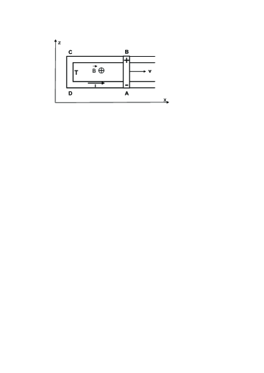
Figure 1: A bar AB of length $a$ moves with constant velocity $\vec{v}$ along the U-shaped frame T in a uniform and constant magnetic field $\vec{B}$, produced by a source at rest in the laboratory and directed along the positive direction of the $y$ axis. The arrow in the low part of the frame indicates the direction of flow of the current $I$.

This thought experiment goes back to Maxwell [3, pp. 218-219]. Conceptually, it can be considered as a version of Faraday’s disc [11] in which the rotation of the disc is substituted by the inertial motion of part of the circuit, thus allowing the use of two inertial reference frames. In the following discussion, it is conventionally assumed that the mobile charges are positive. Because in the laboratory reference frame the vector potential is constant, the induced emf is due only to the line integral $\oint_{l}(\vec{v}_{c}\times\vec{B})\cdot\vec{dl}$ of Eq. (17), and the only portion of the circuit in which it is non-zero is the AB segment. Therefore, the induced emf is given by $\mathcal{E}=-B_{y}va$ (the circulation along the contour is counted as positive when clockwise in fig. 1). The emf is localized in the bar: the bar acts as a battery, with the positive pole at point $B$. The current flows from $A$ to $B$, i.e., from the point at lower potential to that at higher potential, like in a battery. However, for a pair of points on the immobile frame T, the current flows from the point at higher potential to that at lower potential. The concept of localization of the induced emf therefore has physical meaning because it allows the prediction – testable by experiment – of how the potential difference between two points is related to the current flow. If we drop this concept, we decrease the predictive and explanatory power of the theory.

The “flux rule”predicts the correct induced emf. The flux of the magnetic field through the area ABCD is $\Phi=B_{y}avt$, if at $t=0$ the bar AB coincides with the arm DC of the frame. Then:

$$\mathcal{E}=-\frac{d\Phi}{dt}=-B_{y}av,$$ (19)

where the minus sign indicates that the induced current circulates counterclockwise, as indicated in fig. 1. The “flux rule” cannot say where the emf is localized; it can only guess that it might be localized in the bar AB because it is moving (on the grounds that it is the bar’s motion that produces the variation of the magnetic field’s flux and, hence, the induced emf).

However, applying the same argument in the (primed) reference frame of the bar AB, it will be said that the emf is localized in the opposite vertical arm CD of the frame because it is seeing moving away from the bar along the negative direction of the common $x\equiv x^{\prime}$ axis. This statement is false, because, in the reference frame of the bar AB also, the emf is localized in the bar. In fact, at every point of the bar’s reference frame, there is an electric field – due to the fields’ transformation equations (see Appendix A) – given by:

$$E_{z}^{\prime}=\Gamma vB_{y}.$$ (20)

Therefore, an emf $\mathcal{E}^{\prime}=\Gamma vB_{y}a=\Gamma\mathcal{E}$ is induced in the bar. In the arm CD, the effect of the electric field $E_{z}^{\prime}$ on the charges is exactly balanced by the magnetic component of the Lorentz force, and due to the motion ($-v$) of the arm CD in the field $B^{\prime}_{y}=\Gamma B_{y}$. The relation $\mathcal{E}^{\prime}=\Gamma\mathcal{E}$, thus obtained, is a particular case of the more general one treated in Appendix A.

Electric field	Symbol	Value	Direction
Induced	$E_{i}$	$vB$	$\uparrow$
Effective	$E_{e}$	$vBa/l$	$\uparrow$
Electrostatic	$E_{es}$	$vB(1-a/l)$	$\downarrow$

Table 1: Electric fields in the bar. The arrow indicate the direction of the field along the $z$ axis.

If the entire circuit is homogeneous (the frame and the bar are of the same material and have the same section), the physics of the circuit is as follows (see Table 1). At every point of the circuit (bar included), there is a current density given by:

$$J=\frac{E_{e}}{\rho}=\frac{1}{\rho}\frac{vBa}{l},$$ (21)

where $E_{e}$ is an “effective electric field”, $\rho$ the resistivity of the material, and $l$ the length of the entire circuit (frame + bar). In the bar, the effective electric field $vBa/l$ is the sum of two opposing fields: the induced electric field $\vec{E}_{i}=vB\hat{z}$ and an electrostatic field $E_{es}=E_{i}-E_{e}$ directed along the negative direction of the $z$ axis. The origin of this field can be explained as follows. Let us consider the bar moving without touching the frame. The induced electric field $E_{i}=vB$, pushes the positive charges towards the point $B$: this point becomes positively charged, and point $A$ negatively charged. Therefore, an electrostatic field $E_{es}$ directed from $B$ to $A$ is established: this field nullifies the induced electric field in a stationary condition.If the bar slides while touching the frame, a current flows in the circuit: while the induced electric field maintains its original value, the value of the electrostatic field $E_{es}$ diminishes and is such that $E_{es}=E_{i}-E_{e}$ in stationary regime. Finally, it can be easily verified that the field defined as $\vec{E}_{c}=\vec{E}_{e}$ in the frame and as $\vec{E}_{c}=\vec{E}_{es}$ in the moving bar is conservative. This result allows calculating the potential difference between two arbitrary points of the circuit, which is given by the line integral of the conservative electric field between the two points. Naturally, the calculation leads to Ohm’s law, as implied by the starting equation (21), which is Ohm’s law in local form.

The bar we have discussed acts precisely like a battery. The circuital laws are, therefore, similar. We know that complicated chemical reactions take place in a battery. However, its circuital behavior can be described with a model which involves similar $E_{i}$, $E_{e}$, and $E_{es}$. The induced electric field of the bar corresponds to the electromotive field of the battery; the electrostatic field is present in both cases, and in both cases, the effective electric field inside the battery is given by the difference between the previous two.

One must supply mechanical power to keep the bar AB in motion with a constant velocity. If the bars motion is frictionless,this power is equal to the electrical power dissipated in the circuit. Indeed, the electrical power supplied by the electromotive force is given by:

$$W(\mathcal{E})=\mathcal{E}I=\frac{\mathcal{E}^{2}}{R}=\frac{(vBa)^{2}}{R},$$ (22)

where $R$ is the resistance of the circuit. This power is dissipated as heat. For energy conservation, the power supplied by the electromotive force must come from the mechanical work done by the force keeping the bar in motion. If a current $I$ flows in the bar along the positive direction of the $z$ axis, the magnetic field $B$ exerts a force on the bar given by $-IBa\hat{x}$: it tends to slow down the bar. An equal and opposite force must be supplied to the bar to keep it in motion. Its magnitude is given by:

$$F=IBa=\left(\frac{vBa}{R}\right)Ba.$$ (23)

The mechanical power necessary for maintaining the bar in motion is:

$$W(F)=Fv=\frac{(vBa)^{2}}{R}=\frac{\mathcal{E}^{2}}{R}=W(\mathcal{E}).$$ (24)

The fact that the magnetic field $B$ appears in the expression of the electrical power supplied by the induced emf contrasts the fact that, in a vacuum, the magnetic force does not produce work on a moving charge. Here, the magnetic field plays only the role of a mediator between the mechanical force and the electrical power (through the term $\vec{v}_{c}\times\vec{B}$) without yielding any amount of energy.

Let us note that the system described here is quasi-stationary because the length of the frame entering the circuit increases with time.

5 Why the “flux rule” is not a physical law

In this section, we shall compare the general law of electromagnetic induction (17), derived within MLE Electromagnetism, with the “flux rule”(2). Note that the expression of the induced emf (17) contains the vector potential $\vec{A}$, as in Maxwell’s formula (11).

We shall consider a closed conducting filiform loop immersed in a magnetic field and in motion. This loop is not assumed to be rigid, so that it can deform. As is usual, the induced emf can also be written in terms of the magnetic field. Starting from Eq. (15), we write, in the reference frame of the laboratory:

$$\mathcal{E}=\oint_{l}{\vec{E}\,\cdot\,\vec{dl}}+\oint_{l}(\vec{v}_{c}\times\vec{B})\cdot\vec{dl} = \int_{S}\nabla\times\vec{E}\,\cdot\,\hat{n}\,dS+\oint_{l}(\vec{v}_{c}\times\vec{B})\cdot\vec{dl}$$

$$= -\int_{S}\frac{\partial\vec{B}}{\partial t}\,\cdot\,\hat{n}\,dS+\oint_{l}(\vec{v}_{c}\times\vec{B})\cdot\vec{dl},$$

where $S$ is any arbitrary surface that has the closed wire $l$ as contour. We then use the identity, valid for every vector field with null divergence (see, for instance, [16, pp. 10 - 11]:

$$\int_{S}\frac{\partial\vec{B}}{\partial t}\cdot\hat{n}\,dS=\frac{d}{dt}\int_{S}\vec{B}\cdot\hat{n}\,dS+\oint_{l}(\vec{v}_{l}\times\vec{B})\cdot\vec{dl},$$ (26)

where $\vec{v}_{l}$, the velocity of the wire element $dl$, can be different for each wire element. Then, Eq. (5) becomes:

$${\mathcal{E}}=-\frac{d\Phi}{dt}-\oint_{l}(\vec{v}_{l}\times\vec{B})\cdot\vec{dl}+\oint_{l}(\vec{v}_{c}\times\vec{B})\cdot\vec{dl}.$$ (27)

In the case of a rigid, filiform wire moving with velocity $V$ along the positive direction of the common $x^{\prime}\equiv x$ axis, this equation takes the form:

$${\mathcal{E}}=-\frac{d\Phi}{dt}-\oint_{l}(\vec{V}\times\vec{B})\cdot\vec{dl}+\oint_{l}(\vec{v}_{c}\times\vec{B})\cdot\vec{dl}.$$ (28)

This equation is not the “flux rule”. To get it, we must abandon special relativity and try using Galilean relativity. Since $V\ll c$ and $v_{d}\ll c$, we can write: $\vec{v}_{c}=\vec{V}+\vec{v}_{d}$ ($c=\infty)$. Then, we get:

$$\mathcal{E}=-\frac{d\Phi}{dt}+\oint_{l}(\vec{v}_{d}\times\vec{B})\cdot\vec{d}l=-\frac{d\Phi}{dt},$$ (29)

i.e. the “flux rule” (the line integral is null because, for every wire element, the drift velocity of the charges $\vec{v}_{d}$ is parallel to $\vec{dl}$).

In the reference frame of the circuit, we have:

$$\mathcal{E}^{\prime}=-\int_{S^{\prime}}\frac{\partial\vec{B}^{\prime}}{\partial t^{\prime}}\,\cdot\,\hat{n}^{\prime}\,dS^{\prime}+\oint_{l^{\prime}}(\vec{v}^{\prime}_{d}\times\vec{B}^{\prime})\cdot\vec{dl^{\prime}}=-\frac{d}{dt^{\prime}}\int_{S^{\prime}}\vec{B}^{\prime}\cdot\hat{n}^{\prime}dS^{\prime}=-\frac{d\Phi^{\prime}}{dt^{\prime}}.$$ (30)

The “flux rule” – for filiform and rigid circuits – is valid in both reference frames if one uses the Galilean transformation of velocities, namely Galilean relativity ($c=\infty$). Notice that using the Galilean velocity composition is a sufficient condition for the “flux rule”being Galileo-invariant. It is also necessary because, without the Galilean approximation, the “flux rule”cannot even be established: we would have to stop at equation (28). Finally, notice that the “flux rule”is Galileo-invariant at first sight. In the Galilean limit ($c=\infty$) of the relativistic transformations of electric and magnetic fields, $\vec{B}^{\prime}=\vec{B}$. On the other hand, areas and time intervals have the same value in two inertial reference frames. It follows that $d\Phi/dt=d\Phi^{\prime}/dt^{\prime}$, i.e., that the “flux rule”is Galileo invariant and the induced emf has the same value in every inertial frame. How can a Galileo-invariant equation be accepted in a relativistic theory as MLE electromagnetism? These considerations constitute a first argument against the ”flux rule” being a physical law.

Second, let us note that the integral in Eq. (29) is null only if the circuit is filiform. If not, the extension of the material makes $\vec{v}_{d}$ non parallel to the circuit element $\vec{dl}$, and the ”flux rule” is not obeyed. In fact:

$$\mathcal{E}=-\frac{d\Phi}{dt}+\oint_{l}(\vec{v}_{d}\times\vec{B})\cdot\vec{dl}.$$ (31)

Differently from equation (29), the integral is not null owing to the extension of the material.

Third, we would like to emphasize that the general law (17) is a local one. However, the “flux rule” does not satisfy the locality condition. It relates the emf induced in a conducting filiform circuit at time $t$ to the time variation – at the exact same instant $t$ – of the flux of the magnetic field through an arbitrary surface that has the circuit as a contour. Consequently, the “flux rule” cannot be causally interpreted, because what happens at the surface at time $t$ cannot influence what happens in the circuit at the same instant $t$, unless physical interactions can propagate with infinite speed. Moreover, since one can arbitrarily choose the integration surface, we should have endless causes of the same effect: the variation of the flux of the magnetic field through any arbitrary surface, however large, which has the wire as its contour would then be the cause of the induced emf, thus violating, again, the locality condition. As shown above in the case of the moving bar, the “flux rule”, though predicting the correct value of the induced emf, cannot say anything about the physical processes involved or about their causal nature. It is just a mathematical relation between two physical quantities, devoid of physical insight. It can be used, with great care, as a calculation shortcut only when guided by the predictions of the general law.

Moreover, the “flux rule” does not always yield the correct prediction. Indeed, in 1914, André Blondel showed that there could be a flux variation without any induced emf, thus falsifying the “flux rule”[17].

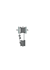
Figure 2: Sketch of Blondel’s experiment testing the “flux rule”. $M_{1}$ and $M_{2}$ are the circular plates of an electromagnet: the magnetic field between the two plates is equal to $0.08$ T and is ‘reasonable uniform’. R is a resistance, and G is a D’Ansorval galvanometer. A and B are two wooden cylinders. The two “r” represent the intersection of a conducting ring attached to cylinder A with the plane of the figure. The two arrows indicate sliding electric contacts. A conducting coil wound around cylinder A, placed within the electromagnet, is unrolled and transferred to cylinder B, where the magnetic field is null.

Blondel used a solenoid wound around a wooden cylinder A placed between the circular armature plates of an electromagnet (Fig. 2). He attached one end of the solenoid to another parallel wooden cylinder B outside the electromagnet (where the magnetic field is null). He then unrolled the solenoid as he transferred the coils from cylinder A to cylinder B, while maintaining the unrolling wire tangent to the two cylinders [17], [18]. According to the “flux rule”, during the transfer of the coil from cylinder A to cylinder B, an emf should be induced in the unrolling solenoid, according to the equation:

$$|\mathcal{E}|=\left|-\Phi_{\rm single\,coil}\frac{dN}{dt}\right|,$$ (32)

where $\Phi_{\rm single\,coil}$ is the magnetic flux through one coil and $N$ the number of coils on cylinder $A$. Since the radius of a coil was $0.1$ m, $B=0.08$ T and $|dN/dt|=6.66$, the emf predicted by (32) is $0.017$ V, well above the detection capability of the D’Ansorval’s galvanometer Blondel used to monitor the current in the circuit. Contrary to what is predicted by the ”flux rule”, the galvanometer showed no deviation [17, 18]. Of course, the general law (17) predicts that in Blondel’s experiment, there is no induced emf. Indeed, the first line integral is null because the vector potential does not depend on time. If, during the unrolling of the solenoid, the unrolling wire is kept tangent to the two cylinders, the second integral is also null because the term $\vec{v}_{c}\times\vec{B}$ has a null component along the wire.

Blondel’s experiment has been rapidly forgotten [20].

6 Why did Maxwell’s general law fall into oblivion?

We have already stressed that the abstract and complicated derivation of Maxwell’s general law may have been an obstacle to its acceptance for his contemporaries (section 2). The elimination of the vector potential by Hertz and Heaviside from Maxwell’s Electromagnetism has very likely contributed to the oblivion of Maxwell’s general law [18]. In particular, one aspect might have had a lasting conceptual impact. Heaviside doubted that the vector potential could have physical meaning: “…[Maxwell] makes use of an auxiliary function, the vector potential of the electric current, and this rather complicates the matter, especially as regards the physical meaning of the process. It is always desirable when possible to keep as near as one can to first principles” [23, p. 46]. Hertz compared the vector potential to a scaffolding that can be removed after the building has been completed. Hertz too was doubtful about the physical meaning of the vector potential: “…one would expect to find in these [fundamental] equations relations between the physical magnitudes which are actually observed, and not between magnitudes which serve for calculations only” [24].

However, other factors may have contributed, and in particular the role played by textbooks. In his The Structure of Scientific Revolutions, Thomas Kuhn has stressed the primary role played by textbooks in transmitting the acquired knowledge to new generations [25]. To verify the role played by textbooks in the oblivion of Maxwell’s general law, we have analyzed eleven university textbooks – considered representative due to their authors or their popularity. Here is a concise overview; one can find the detailed analysis in [9].

In all these textbooks, the treatment of induction begins with the presentation of a series of Faraday’s experiments, distinguishing between those involving the relative motion of a magnet and a circuit (magneto-electric induction, in Faraday’s language) and those in which the induced current is due to the current variation in another circuit (volta-electric induction). The theoretical description of these phenomena varies greatly, ranging from the elementary treatment by Riecke [26], to the more sophisticated ones involving the relativistic nature of Electromagnetism [27, 28].

Except for Feynman’s Lectures [4], Zangwill’s [16], and Griffiths’ [19]] texts, all these textbooks refer to the “flux rule” as the “law of electromagnetic induction”. These texts adhere, knowingly or not, to the introductory part of Maxwell’s discussion of electromagnetic induction and ignore his general law.

Indeed, a typical theoretical treatment (see for instance [28, p. 233]) is based on the definition of the induced emf as:

$$\mathcal{E}_{C}=\oint_{l}\vec{E}\cdot\vec{dl}.$$ (33)

This definition stems from the electrostatic law $\vec{F}=q\vec{E}$, and it leads to the correct result only if applied in the reference frame of a rigid filiform circuit. It cannot be used when the circuit moves.

By using Stokes’ theorem and Maxwell’s equation:

$$\nabla\times\vec{E}=-\frac{\partial\vec{B}}{\partial t},$$ (34)

it is found that:

$$\mathcal{E}_{C}=\oint_{l}\vec{E}\cdot\vec{dl}=\int_{S}\nabla\times\vec{E}\cdot\hat{n}\,dS=-\int_{S}\frac{\partial\vec{B}}{\partial t}\cdot\hat{n}\,dS=-\frac{d}{dt}\int_{S}\vec{B}\cdot\hat{n}\,dS,$$ (35)

namely, the “flux rule”. Notice that the last equality is valid only if the filiform and rigid circuit is at rest.

Another type of approach consists in stating the “flux rule” as a law inferred from experiments – as Maxwell did as a first step – and exploring how it effectively deals with many experimental situations. Within this approach, starting from the “flux rule”, the differential Maxwell’s equation of the curl of the electric field is derived [13, p. 80]; [30, pp. 158-159]; [31, pp. 158-159].

Modern textbooks widely use the vector potential to calculate the effects of currents or magnets. Nevertheless, they do not use the vector potential to treat electromagnetic induction: see, for instance, [16, pp. 462-463]. This choice implicitly does not make any distinction between equations that obey the locality condition and those that don’t. The general law of electromagnetic induction belongs to the former; the “flux rule” to the latter.

7 Teaching issues

Teaching the modern formulation of Maxwell’s general law in advanced courses poses no problems. However, it may be more difficult in high schools or elementary physics courses [32]. Here, we suggest a way of introducing Maxwell’s general law and the vector potential by using Faraday’s well-known experiment, commonly reproduced in didactic laboratories: the relative motion of a magnet and a rigid, filiform coil (see Appendix A). [33] describes a laboratory session in which, starting from the autonomous experimenting by students, the general law of electromagnetic induction is obtained through a collective discussion that is guided, when necessary, by the instructor.

The starting point for the theoretical description of the (thought) experiment should be the definition of the induced emf given by Eq. (15). Instructors should adapt the formalism to their teaching contexts, while keeping two cornerstones: the necessity of describing the phenomenon in the two reference frames and that of a local description in the coil’s reference frame.

Eq. (17) is written step by step by asserting that a physical law must have the same form in every inertial frame. Our proposal derives the expression of the electric field entering the definition (15), thus obtaining the modern formulation of Maxwell’s general law. It must be stressed that Eq. (17) will not be derived but only reasonably guessed.

In the reference frame of the magnet, the magnetic field is constant, and there is no electric field.Therefore, the induced emf can be due only to a term $\vec{V}\times\vec{B}$, as suggested by the magnetic component of the Lorentz force ($\vec{V}$ is the velocity of the coil with respect to the magnet):

$$\mathcal{E}=\oint_{l}(\vec{V}\times\vec{B})\cdot\vec{dl}.$$ (36)

In the reference frame of the coil, the induced current must be due to an electric field $\vec{E}^{\prime}$ such that:

$$\mathcal{E}^{\prime}=\oint_{l^{\prime}}\vec{E}^{\prime}\cdot\vec{dl^{\prime}}=-\frac{d}{dt^{\prime}}\int_{S^{\prime}}\vec{B}^{\prime}\cdot\hat{n}^{\prime}dS^{\prime}.$$ (37)

Following Maxwell [3, pp. 27-28] ), we write this equation in terms of a vector defined at each point of the coil: this will ensure the locality of the phenomenon. Let us denote this vector $\vec{A}^{\prime}$ and call it “vector potential”:

$$\mathcal{E}^{\prime}=\oint_{l^{\prime}}\vec{E}^{\prime}\cdot\vec{dl^{\prime}}=-\frac{d}{dt^{\prime}}\int_{S^{\prime}}\vec{B}^{\prime}\cdot\hat{n}^{\prime}dS^{\prime}=-\frac{d}{dt^{\prime}}\oint_{l^{\prime}}\vec{A}^{\prime}\cdot\vec{dl^{\prime}}.$$ (38)

Naturally, this is Maxwell’s Eq. (7). Because the integration line does not depend on time, the above equation assumes the form:

$$\mathcal{E}^{\prime}=\oint_{l^{\prime}}\vec{E}^{\prime}\cdot\vec{dl^{\prime}}=\oint_{l^{\prime}}\left(-\frac{\partial\vec{A}^{\prime}}{\partial t^{\prime}}\cdot\vec{dl^{\prime}}\right).$$ (39)

Because a physical law must be valid in every inertial frame, we conclude that the law of electromagnetic induction should be written as a combination of Eq. (36) and (39), i.e. as:

$$\mathcal{E}^{\prime}=\oint_{l^{\prime}}\left[-\frac{\partial\vec{A}^{\prime}}{\partial t^{\prime}}+(\vec{V}\times\vec{B}^{\prime})\right]\cdot\vec{dl^{\prime}}.$$ (40)

This equation is valid in both reference frames: the second term of the integral operates in the magnet’s reference frame; the other in the coil’s frame. At this point, one should recall that Eq. (40) is valid also if, instead of a moving magnet, we have a primary circuit in which a variable current flows: see Appendix A and the discussion of Purcell and Morin’s textbook in [9].

From this point on, instructors can refine the proposal according to their teaching contexts, having in mind the complete treatment of section 3. One could introduce the distinction between the velocity of the coil and that of the charges contained in it. As for the expression between the two square brackets of Eq. (40), the instructor could generalize it by adding the term $-\nabla\varphi$.

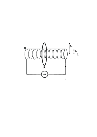
Figure 3: Induction between a ring $R$ and a solenoid $S$ through which flows a low frequency alternating current $I$. See also [18, 29]

.

By considering the apparatus of fig. 3, one can derive the expression of the vector potential in an exemplar case. A low frequency alternating current $I$ flows in a long solenoid S of radius $a_{S}$, thus creating a time-varying magnetic field. In the case of an ideal solenoid (constituted by an infinite array of circular coils), the magnetic field outside the solenoid is null, whereas $\vec{B}=\mu_{0}nI\hat{z}$ inside the solenoid, with $n$ the number of turns per unit length of the solenoid, and $\hat{z}$ the unit vector along the solenoid’s symmetry axis.

According to the law (40), the emf induced in the filiform ring is given by:

$$\mathcal{E}=-\oint_{R}\frac{\partial\vec{A}}{\partial t}\cdot\vec{dl}=-\frac{d}{dt}\oint_{R}\vec{A}\cdot\vec{dl}=-2\pi a_{R}\frac{dA}{dt},$$ (41)

where $a_{R}$ is the radius of the ring. The induced emf can also be written as:

$$\mathcal{E}=-\frac{d}{dt}\int_{\mathcal{S}}\vec{B}\cdot\hat{n}\,d\mathcal{S}=-\mu_{0}n\pi a_{S}^{2}\frac{dI}{dt},$$ (42)

where ${\mathcal{S}}$ is an arbitrary surface that has the ring as contour. By equating the last members of the two equations above, we get:

$$A=\mu_{0}\frac{na_{S}^{2}}{2a_{R}}I,$$ (43)

where the constant of integration is taken to be to zero to obtain a vector field that vanishes far from the source. The vector potential has the same absolute value at every point of the ring and the induced emf is distributed homogeneously along the ring: the ring acts as a source of current. Taking two points $M$ and $N$ on the ring, we have the electric potential difference:

$$\varphi_{M}-\varphi_{N}=\mathcal{E}\frac{\Delta\alpha}{2\pi}-i\Delta R=\mathcal{E}\frac{\Delta\alpha}{2\pi}-\frac{\mathcal{E}}{R}\left(R\frac{\Delta\alpha}{2\pi}\right)=0,$$ (44)

where $i$ is the induced current, $\Delta R$ the resistance of the $MN$ arc and $\Delta\alpha$ its angle. The filiform ring is an equipotential line.

Eq. (43) shows that the sources of the vector potential are the currents – namely charges in motion – as it is for the magnetic field. Eq. (39) shows that the vector potential (i.e., the charges in motion) contributes to the value of the electric field through its partial derivative with respect to time. On the other hand, Eq. (38) establishes a relation between the vector potential and the magnetic field, at the same instant, in different regions of space: a line and an arbitrary surface that has the line as a contour. The arbitrariness of the choice of the integration surface suggests a strong spatial relationship between the vector potential and the magnetic field: instructors know that $\vec{B}=\nabla\times\vec{A}$ and, depending on the teaching context, can communicate to the students the explicit form of this equation or its essential feature (dependence of the magnetic field on the spatial partial derivatives of the vector potential components). In other words, the vector potential depends both on the spatial coordinates and on time. The dependence on the coordinates relates the vector potential to the magnetic field; the dependence on time, relates the vector potential to the electric field.

To wind it all up, the instructor should discuss again the issue of the transition from the conceptual framework of the action at a distance to a field description of electromagnetic phenomena. In addition to the path going from the existence of a charge to the explanation of the force between two charges (charge $\rightarrow$ fields $\rightarrow$ force on another charge), there is another one according to which charges create potentials that give rise to fields and, in turn, to a force exerted on other charges (charge $\rightarrow$ potentials $\rightarrow$ fields $\rightarrow$ force on another charge). Here, we have an example of how physicists use mathematics to build increasingly abstract theories, but which are, sometimes – as in the case of the potentials – more apt at dealing with the intrinsic Lorentz invariance of Maxwell’s electromagnetism.

8 Conclusions

The rooting and the persistence of the “flux rule”appear to be an example of the collective processes studied by Ludwik Fleck in his Genesis and Development of a Scientific Fact, first published in German in 1935 [34, p. 27]]:

Once a structurally complete and closed system of opinions consisting of many details and relations has been formed, it offers enduring resistance to anything that contradicts it.

[…]

What we are faced with here is not so much simple passivity or mistrust of new ideas as an active approach which can be divided into several stages. (1) A contradiction to the system appears unthinkable. (2) What does not fit into the system remains unseen; (3) alternatively, if it is noticed, either it is kept secret, or (4) laborious efforts are made to explain an exception in terms that do not contradict the system. (5) Despite the legitimate claims of contradictory views, one tends to see, describe, or even illustrate those circumstances which corroborate current views and thereby give them substance.

In our opinion, this description fits to a large extent the case of the “flux rule”. Textbooks played a fundamental role in this process. Understanding this role and bringing to the surface its main traits would require a study encompassing physics, epistemology, and social behaviors. It goes beyond the aims of this paper and our competence. We can only underline some aspects of the issue. Generally, a rooted theoretical description of some phenomena is shaken when a new experimental result contrasts the accepted view. In the case of the “flux rule”, Blondel’s experiment should have put it under fire. However, this did not happen. Thomas Kuhn has described the resistance of an acquired view against experimental results that undermine it. Generally, the change of an acquired view is provoked by a series of new experimental results and/or by a radical change in a broader theoretical contest. Einstein’s relativistic electromagnetism should have played this role. Nevertheless, it did not. Indeed, textbooks sometimes touch on this issue but do not wholly develop its consequences to the point of asking: what invariancy is satisfied by the “flux rule”? Moreover, if it emerges that the “flux rule”is Galileo-invariant, how can it be tolerated in a wholly relativistic theory? Another critical issue is constituted by the historical falsehoods encountered in many texts. These falsehoods are possible because textbook writers do not check their statements with historical records but adhere to some anonymous historical tradition. This habit amounts to dismissing the cultural role of historical studies. Historical falsehoods can also distort physics. This issue should also be explored from a sociological point of view. Finally, it seems clear that the lack of an epistemological commitment favors the tradition’s persistence.

Acknowledgements. I want to thank Biagio Buonaura for the many helpful discussions on this subject. The comments and suggestions of the two anonymous Referees have also contributed to giving the paper its final form.

Appendix A Lorentz invariance of the general law of electromagnetic induction

Let us consider a magnetic field source at rest in the laboratory reference frame. A filiform, rigid circuit moves with velocity $V$ along the positive direction of the common $x\equiv x^{\prime}$ axis. In the circuit’s reference frame, the general law (17) assumes the form:

$${\mathcal{E}^{\prime}}=\oint{\vec{E}^{\prime}\cdot\vec{dl^{\prime}}}+\oint(\vec{v}^{\prime}_{d}\times\vec{B}^{\prime})\cdot\vec{dl^{\prime}},$$ (45)

where $\vec{v}_{d}^{\prime}$ is the drift velocity of the charges. The second integral is null because the drift velocity is parallel to $\vec{dl^{\prime}}$ in every circuit element, so that we are left with the first line integral. Taking into account the field’s transformation:

$$E^{\prime}_{x} = E_{x}$$

$$E^{\prime}_{y} = \Gamma[E_{y}+(\vec{V}\times\vec{B})_{y}]$$

$$E^{\prime}_{z} = \Gamma[E_{z}+(\vec{V}\times\vec{B})_{z}],$$

where $\Gamma=1/\sqrt{1-V^{2}/c^{2}}$, and the coordinates transformations:

$$dx^{\prime} = \Gamma dx$$

$$dy^{\prime} = dy$$

$$dz^{\prime} = dz,$$

we get:

$$\mathcal{E}^{\prime} = \Gamma\oint E_{x}dx+\Gamma\oint[E_{y}+(\vec{V}\times\vec{B})_{y}]dy+\Gamma\oint[E_{z}+(\vec{V}\times\vec{B})_{z}]dz$$

$$= \Gamma\oint[\vec{E}+(\vec{V}\times\vec{B})\cdot\vec{dl}].$$

In the laboratory reference frame, we have:

$$\mathcal{E}=\oint(\vec{E}+\vec{V}\times\vec{B})\cdot\vec{dl}.$$ (47)

Hence:

$$\mathcal{E}^{\prime}=\Gamma\mathcal{E}.$$ (48)

We have thus shown that the phenomenon of electromagnetic induction, involving electric and magnetic fields, must be treated relativistically, as claimed by Einstein [15]. Provided that the relative velocity is such that $V\ll c$, we can assume $\Gamma\simeq 1$, and the predicted value of $\Gamma$ differs from $1$ by an experimentally not detectable amount.

References

- [1] M. Faraday, Experimental Researches in Electricity vol. I, pp. 1-16 (Taylor, London, 1839).
- [2] E . Lenz, “Über die Bestimmung der Richtung der durch elektrodynamische Vertheilung erregten galvanischen Ströme,” Ann. Phys. Chem. 31 483-494 (1834).
- [3] J. C. Maxwell, A Treatise on Electricity and Magnetism vol. II sec. ed. (Clarendon Press, Oxford, 1881).
- [4] R. Feynman, R. Leighton and M. Sands, The Feynman lectures on Physics vol. II pp. 17.1-17.3 (Addison - Wesley, Reading, 1963).
- [5] A. D. Yaghjian, “Maxwell’s derivation of the Lorentz force from Faraday’s law,” Progress In Electromagnetics Research M, 93, 35-42 (2020).
- [6] H. Bouasse, Cours de Magnétisme et d’Électricité - Première Partie - Étude du Champ Magnétique (Delagrave, Paris, 1914), online here.
- [7] J. C. Maxwell, A Treatise on Electricity and Magnetism vol. I 2nd. ed. (Clarendon Press, Oxford, 1881).
- [8] Indeed, this symbol replaces, for technical reasons, the symbol used by Maxwell in [7, p. 72].
- [9] See the script in supplementary material at Supplementary material.
- [10] B. J. Hunt, “Oliver Heaviside: A first-rate oddity”, Phys. Today 65 48-54 (2012).
- [11] G. Giuliani, “A general law for electromagnetic induction,” EPL 81 60002 (2008).
- [12] The name “electromotive force” is misleading, because, as we know, the electromotive force is not a force: it has the dimensions of an electric potential, and it is measured in volts. Since a more suitable name has not been invented, we shall keep on using the same name. It is worth noting that, today’s use of some historical names appears to have no justification. For instance, we find that the magnetic field , recovering a nineteenth century’s denotation, is called “magnetic induction vector”; and the field , whose sources are the current densities , is called “magnetic field”. Then one has to stress that what appears in the expression of the Lorentz force is the magnetic induction vector and not the magnetic field. Let us also mention the conceptual confusion created by the habit of recalling the contributions of different researchers in the name of a formula, a habit that often badly distorts history. For instance, as for the “flux rule”, we have encountered the denomination “Faraday - Neumann - Lenz law”, or variants at will. The presence of Lenz is justified by the sign (-) that appears in the formula, but Faraday and Neumann have nothing to do with the “flux rule”.
- [13] J. C. Slater and N. H. Frank, Electromagnetism (McGraw - Hill, New York, 1947).
- [14] As it is well known, an equation is local if it relates physical quantities at the same point at the same instant, or if it relates physical quantities in two distinct points at two successive instants , provided that the distance between the two points satisfies the equation: . This locality condition is necessary but not sufficient for interpreting an equation causally. For instance, let us consider the law . As the momentum varies over time, we are inclined to interpret this equation by saying that the force ‘causes’ the momentum variation. However, there are situations where the change in momentum ‘causes’ a force. Consider, for example, a completely absorbing surface hit perpendicularly by a monochromatic beam of light directed along the negative direction of the axis. In this case, if is the number of photons absorbed per unit time, the surface momentum obeys: , and we can say that the variation of the photons’ momentum has produced a radiative force on the surface . A similar situation is found in the kinetic theory of gases: the pressure (force per unit area) on the walls is due to the exchange of momentum with the particles.
- [15] A. Einstein, “Zur Electrodynamik bewegter Körper,” Ann. Phys. 17 891 - 921 (1905), English. trans. in The collected papers of Albert Einstein vol 2 (Princeton, NJ: Princeton University Press) 140 - 171 p. 140.
- [16] A. Zangwill, Modern Electrodynamics (Cambridge University Press, Cambridge, 2013).
- [17] A. Blondel, “Sur l’énoncé le plus general des lois de l’induction,” Compt. Rend. Ac. Sc. 159 674 - 679 (1914).
- [18] G. Giuliani, “Vector potential, electromagnetic induction and ‘physical meaning’,” Eur. J. Phys. 31 871 - 880 (2010).
- [19] D. J. Griffiths, Introduction to Electrodynamics 4th ed. (Pearson, Boston, 2013).
-
[20]
The above discussion reminds us of another question.