The role of thermal fluctuations in the motion of a free body

Abstract

The motion of a rigid body is described in Classical Mechanics with the venerable Euler’s equations which are based on the assumption that the relative distances among the constituent particles are fixed in time. Real bodies, however, cannot satisfy this property, as a consequence of thermal fluctuations. We generalize Euler’s equations for a free body in order to describe dissipative and thermal fluctuation effects in a thermodynamically consistent way. The origin of these effects is internal, i.e. not due to an external thermal bath. The stochastic differential equations governing the orientation and central moments of the body are derived from first principles through the theory of coarse-graining. Within this theory, Euler’s equations emerge as the reversible part of the dynamics. For the irreversible part, we identify two distinct dissipative mechanisms; one associated with diffusion of the orientation, whose origin lies in the difference between the spin velocity and the angular velocity, and one associated with the damping of dilations, i.e. inelasticity. We show that a deformable body with zero angular momentum will explore uniformly, through thermal fluctuations, all possible orientations. When the body spins, the equations describe the evolution towards the alignment of the body’s major principal axis with the angular momentum vector. In this alignment process, the body increases its temperature. We demonstrate that the origin of the alignment process is not inelasticity but rather orientational diffusion. The theory also predicts the equilibrium shape of a spinning body.

I Introduction

Understanding how a body moves in space is a central problem in Classical Mechanics, with strong implications in astrophysics ranging from the dynamics of interstellar dust Lazarian (2007), to asteroid dynamics Efroimsky and Lazarian (2000); Efroimsky (2001); Warner et al. (2009); Breiter et al. (2012); Frouard and Efroimsky (2018) and the motion of the Earth Souchay et al. (2003); Chen and Shen (2010), among others. At the scale of the laboratory, the field of levitodynamics aims to control levitated nano- and micro-objects in vacuum Gonzalez-Ballestero et al. (2021). These systems provide exquisite sensors for torques, forces, and accelerations Prat-Camps et al. (2017); Ricci et al. (2019), as well as help unravel fundamental questions in quantum physics Millen and Stickler (2020), and the stochastic thermodynamics of small systems Gieseler et al. (2014). Given the small size of the bodies involved, understanding the interplay of dissipation and thermal fluctuations is a crucial issue, treated phenomenologically so far van der Laan et al. (2020).

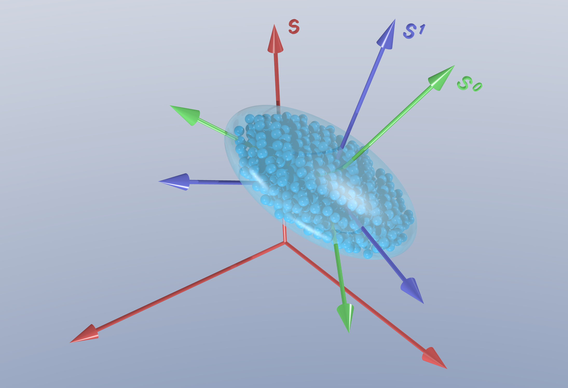
Figure 1: A body made of moving bonded atoms (little blue spheres) is coarse-grained with the gyration tensor, represented here with a translucent ellipsoid. Also shown are the inertial lab frame ${\cal S}$ (red), the principal axis non-inertial frame ${\cal S}^{0}$ (green), and the zero angular momentum non-inertial frame ${\cal S}^{1}$ (blue).

The starting point for describing the motion of a rigid body in Classical Mechanics are Euler’s equations. A rigid body is an idealization for a system of classical particles that assumes the relative distances among them are constant in time Goldstein (1983); V. I. Arnold (1989). Under this assumption, there are reference systems in which all the particles are at rest. Euler obtained the equations from the relationship between two orthogonal reference systems in motion, the observation that the inertia tensor diagonalizes in the principal axis reference system, and the conservation laws, in particular that of angular momentum Descamps (2008); Gautschi (2008).

In reality the particles in a solid object (sketched in Fig. 1) at finite temperature are moving and oscillating very rapidly around their equilibrium positions and have no fixed relative distances. The dynamics of the particles is governed classically by Hamilton’s equations. To our knowledge, the conceptual gap between Hamilton’s equations for the particles of a body and Euler’s equations for a rigid body has not yet been closed. We aim at deriving the equations for a rigid body directly from Hamilton’s equations of the evolving interacting particles that constitute the body, without recourse to the rigid body idealization. This is not only a pleasant intellectual achievement, but also sheds light on the behaviour of realistic systems where the rigid body idealization is not accurate. As an example, we identify a dissipative mechanism not considered so far, that of orientational diffusion, which turns out to be the one actually responsible for the alignment of rotating bodies. Also, as thermal fluctuations are important in molecular systems, and on many occasions molecules or portions of molecules Goujon et al. (2020) are treated as rigid entities, a clarification of the interplay between rigidity and thermal fluctuations is important in these systems. In fact, the modelling of a body made of atoms in terms of constraints (like constant distances between atoms) is subtle and problematic Fixman (1974, 1978); van Kampen (1981); Español et al. (2011).

A number of works have treated orientation and shape variables for deformable bodies in Classical Mechanics Guichardet (1984); Shapere and Wilczek (1989); Littlejohn and Reinsch (1997). They coordinate transform the $n$-body problem into two distinct sets that capture the overall orientation and the shape. In this approach, the freedom in choosing the body frame leads to gauge invariance, and to an interesting mathematical structure Shapere and Wilczek (1989). The theory allows one to understand how a closed path in shape space leads to an overall rotation, explaining how a falling cat can maneuver its internal degrees of freedom to land on its feet, or how a torque-free trampolinist can perform turns in the air. The fact a deformable body may rotate in the absence of angular momentum has been observed recently in very small molecular systems Katz and Efrati (2019), and has also provided examples of a classical time crystal Peng et al. (2021). However, these microscopic theories do not obtain closed equations for the “macroscopic shape” as captured by, for example, the principal moments of the body.

A different approach is given from the point of view of rational continuum mechanics in the so called theory of pseudo-rigid bodies Cohen and Muncaster (1988),O’Reilly and Thoma (2003). In this theory, a body is characterized as a zero dimensional directed continuum consistent with non-linear elasticity theory. In that respect such a theory is a coarse version of a continuum theory. Being formulated at an abstract level, the statistical mechanics underpinning of the theory of pseudo-rigid bodies is lacking. Dissipation is also lacking in this approach.

There are recent attempts to introduce stochasticity and dissipation in rigid body dynamics, from the point of view of geometric mechanics Castro and Arnaudon (2017); Arnaudon et al. (2018). In this mathematically oriented approach, a stochastic dynamics for the angular momentum vector is proposed. Physically, this means the solid body is interacting with a bath of particles, otherwise, the angular momentum would be conserved. In fact, the literature on so-called Brownian rotors, that is, rigid bodies immersed in a fluid and experiencing thermal fluctuations arising from collisions with fluid molecules, is extensive Galkin and Rusakov (2008); Walter et al. (2010); Shrestha et al. (2015); Martinetz et al. (2018), dating back to the relaxation model of Debye. The thermal fluctuations considered in the present paper are, however, of a very different nature from those of Brownian rotors. They do not arise from an external bath, but from eliminated degrees of freedom of the body in favor of the coarse-grained (CG) variables. The dissipation is “internal”, the body is isolated, and angular momentum and total energy are conserved in our work.

The way we proceed in order to derive the equations of motion for a quasi-rigid body is based on non-equilibrium statistical mechanics Green (1952); Zwanzig (1961); Grabert (1982). This is a theory of coarse graining that provides the tools for the reduction of all the information about rapidly varying atomic variables to a few variables governing the behaviour of the system as a whole. Typically, the selected coarse-grained (CG) variables are assumed to be slow on the atomic time scale, thus allowing for a description of their evolution as an overall slow motion with superimposed small rapid fluctuations modelled as white noise. The theory of coarse-graining provides the Fokker-Planck Equation (FPE) for the evolution of the non-equilibrium probability distribution of the CG variables, and its associated stochastic differential equation (SDE). The drift and diffusion terms of the FPE and SDE are given in terms of conditional expectations over the microscopic degrees of freedom and are, therefore, fully expressed in microscopic terms. Thermal fluctuations are naturally described in this approach and, concomitant with them, the CG description fully describes dissipation which is in agreement with the Second Law. In the limit of small fluctuations, valid for macroscopic bodies, the approach leads to deterministic equations.

In this work, we coarse-grain a free body by using the eigenvalues and eigenvectors of the gyration tensor as the coarse variables, from which the stochastic differential equations governing the dynamics of the orientation and central moments of a free body are derived. These equations generalize Euler’s equations for a free solid body by taking into account deformation, dissipation, and thermal fluctuations. The original Euler’s equations turn out to be just the reversible part of the whole dynamics. Therefore, to our knowledge, this constitutes the first derivation of Euler’s equations from Hamilton’s equations. We make explicit two crucial but questionable assumptions in Euler’s treatment. First, we distinguish between the spin velocity, related to the angular momentum, and the angular velocity, related to the rotation of the principal axis frame. These two quantities are assumed to coincide in a rigid body, but they are different in a real body. This difference is at the heart of orientational dissipation in the system. Second, we describe an additional source of dissipation due to the unavoidable deformation (non-constant principal moments) of a real body that can be identified with viscoelasticity.

The SDE obtained in this work predicts the rotating body will follow a Brownian motion that directs the orientation towards the maximum entropy state, in accordance with the Second Law. In this state, the body’s principal axis with the largest moment aligns with the conserved angular momentum vector, an effect known as precession relaxation Frouard and Efroimsky (2018) and also as nutation damping Sharma et al. (2005). This effect is predicted from equilibrium thermodynamics (see §26 of Ref. Landau and Lifshitz (1980)) but the present theory describes the evolution towards the maximum entropy equilibrium state. The need to include dissipation in the dynamics of rotating bodies arises very explicitly in the description of rotating astronomical objects like interstellar dust, asteroids, and satellites. The vast majority of asteroids, for example, are in pure rotation Lamy and Burns (1972); Warner et al. (2009); Breiter et al. (2012). Previous approaches describing the alignment process and estimating the corresponding relaxation times are based on the idea that inelastic relaxation arises from alternating elastic stresses generated inside a wobbling body by the transversal and centripetal acceleration of its parts. The alternate stresses deform the body, and inelastic effects cause energy dissipation Prendergast (1958); Efroimsky et al. (2002); Sharma et al. (2005); Sharma (2017); Kwiecinski (2020). At the coarser level of description selected in the present work, based on the gyration tensor, the alignment of a free body towards pure rotation is captured through orientational diffusion, while dilational friction – that would represent viscoelasticity at this level of description– is seen to play no role in the mechanism of precession relaxation.

The paper is structured as follows. In Sec. II we review the Classical Mechanics for the motion of a free body from the point of view of Hamiltonian dynamics. This allows us to set the notation and pinpoint subtle issues appearing in the rigid body idealization, as elaborated in Sec. III where we also announce the generalization of Euler’s equations including dissipation. In Sec. V we summarize the theory of coarse-graining used in the present work. Section  VI discusses the CG variables used at the present level of description. Sections VII-X present the different building blocks entering into the SDE governing the motion of a free solid body. We are able to formulate all the terms in such a way that they are either analytically known, can be computed explicitly by MD simulations, or eventually fitted from observations of real systems. The final form of the SDE is given in Sec. XI, with a summary of the approximations in Sec. XII. The physical interpretation of the different terms is presented in Sec. XIII, and discussion and conclusions are presented in Sec. XIV. The calculations involved in the evaluation of the different building blocks, along with some instrumental mathematical results, are presented as Supplemental Material SM.

II Review of Hamiltonian dynamics for a body made of bonded particles

In order to set the notation, in this section we review the Classical Mechanics for a system of particles interacting with an interparticle potential but otherwise free from external forces.

Let $z=\{r,p\}=\{{\bf r}_{i},{\bf p}_{i},i=1,\cdots,N\}$ be the set of microscopic degrees of freedom for a body with $N$ particles, where ${\bf r}_{i}$ is the position of particle $i$ and ${\bf p}_{i}$ its momentum. We will refer to $z$ as the microstate and $r$ as the configuration. The set of all $z$ constitutes the phase space. The degrees of freedom $z$ are defined with respect to an inertial reference frame ${\cal S}$ in which Hamilton’s equations are valid. We assume the Hamiltonian of the system to be of the usual form

$$\hat{H}(z) =\sum_{i}^{N}\frac{{\bf p}_{i}^{2}}{2m_{i}}+\hat{\Phi}(r)$$ (1)

with the potential of interaction $\hat{\Phi}(r)=\hat{\Phi}({\bf r}_{1},\cdots,{\bf r}_{N})$. In this work, circumflexed symbols denote functions in phase space. The Hamiltonian is a dynamic invariant, as are the linear and angular momenta of the system. When the total linear momentum is zero, the center of mass position is also a dynamic invariant.

We introduce the first geometrical moments of the distribution of particles, which are the total mass ${\rm M}$, the center of mass position $\hat{\bf R}$, and the tensor of inertia $\hat{\bf I}$ of the body. These phase functions depend on the position of the particles but not on their momenta. They are given by

$${\rm M} \equiv\sum^{N}_{i}m_{i}$$

$$\hat{\bf R} \equiv\frac{1}{M}\sum^{N}_{i}m_{i}{\bf r}_{i}$$

$$\hat{\bf I} \equiv\sum^{N}_{i}m_{i}[{\bf r}_{i}-\hat{\bf R}]_{\times}^{T}\!\cdot\![{\bf r}_{i}-\hat{\bf R}]_{\times}$$ (2)

where the superscript $T$ denotes the matrix transpose. The cross product matrix $[{\bf A}]_{\times}$ is defined as the antisymmetric matrix constructed from an arbitrary vector ${\bf A}=({\bf A}^{x},{\bf A}^{y},{\bf A}^{z})$ as

$$[{\bf A}]_{\times} =\left(\begin{array}[]{ccc}0&-{\bf A}^{z}&{\bf A}^{y}\\ {\bf A}^{z}&0&-{\bf A}^{x}\\ -{\bf A}^{y}&{\bf A}^{x}&0\end{array}\right)$$ (6)

or in component form $[{\bf A}]_{\times}^{\alpha\beta}=\sum_{\gamma}\epsilon^{\alpha\gamma\beta}{\bf A}^{\gamma}$, where $\epsilon^{\alpha\gamma\beta}$ is the Levi-Civita symbol. Expression (2) for the inertia tensor is identical to the usual definition given by

$$\hat{\bf I} =\sum_{i}m_{i}\left[\left({\bf r}_{i}-\hat{\bf R}\right)^{2}\mathbb{1}-\left({\bf r}_{i}-\hat{\bf R}\right)\left({\bf r}_{i}-\hat{\bf R}\right)^{T}\right]$$ (7)

where $\mathbb{1}$ is the identity matrix. However, form (2) is more convenient in explicit calculations. It also shows manifestly that the inertia tensor is symmetric and positive definite.

The linear momentum $\hat{\bf P}$ and spin $\hat{\bf S}$ of the system are

$$\hat{\bf P} \equiv\sum_{i}{\bf p}_{i}$$

$$\hat{\bf S} \equiv\sum_{i}\left({\bf r}_{i}-\hat{\bf R}\right)\times{\bf p}_{i}$$ (8)

The spin is the angular momentum of the body with respect to the center of mass of the body. It is convenient to define the linear velocity $\hat{\bf V}$ and spin velocity $\hat{\boldsymbol{\Omega}}$ of the body as

$$\hat{\bf V} \equiv{\rm M}^{-1}\hat{\bf P}$$

$$\hat{\boldsymbol{\Omega}} \equiv\hat{\bf I}^{-1}\!\cdot\!\hat{\bf S}$$ (9)

We refer to $\hat{\boldsymbol{\Omega}}$ as the spin velocity and not as the angular velocity because the latter name is reserved for the angular velocity $\hat{\boldsymbol{\omega}}$ of the principal axis frame with respect to the lab frame, as defined below. These two phase functions are different in general.

Throughout this work and in the Supplementary Material, vectors, matrices or tensors are rendered in bold font ${\bf A}$, with diagonal matrices additionally rendered with voided fonts $\mathbb{A}$. Indices representing Cartesian components of these quantities appear in Greek font either as subscripts or superscripts, while those representing particle number appear as subscripts in Roman font. Unless stated otherwise or shown explicitly, repeated indices are assumed to be summed over, that is the Einstein convention is employed, unless the indices are underlined, in which case no summation is implied.

II.1 The orientation and principal moments

Because the inertia tensor is a symmetric positive definite matrix it can be diagonalized. The principal axis system ${\cal S}^{0}$ is defined as the reference system with origin at the center of mass in which the inertia tensor diagonalizes. Let the basis vectors of the inertial laboratory reference system ${\cal S}$ and the non-inertial principal axis reference system ${\cal S}^{0}$ be denoted by $\hat{\bf e}_{\alpha}$, and $\hat{\bf e}^{0}_{\alpha}$, respectively, with $\alpha=1,2,3$. The components of the rotation matrix of ${\cal S}^{0}$ with respect to ${\cal S}$ are defined as

$$\hat{\boldsymbol{\cal R}}_{\alpha\beta} ={\bf e}^{T}_{\beta}\!\cdot\!\hat{\bf e}^{0}_{\alpha}$$ (10)

In ${\cal S}^{0}$ the inertia tensor takes the form

$$\hat{\boldsymbol{\cal R}}\!\cdot\!\hat{\bf I}\!\cdot\!{\hat{\boldsymbol{\cal R}}}^{T} =\hat{\mathbb{I}}$$ (11)

where $\hat{\mathbb{I}}$ is a diagonal matrix whose elements are the principal moments $\hat{I}_{1},\hat{I}_{2},\hat{I}_{3}$. Note that $\hat{\bf e}^{0}_{\alpha}$ are the normalized eigenvectors of the inertia tensor.

The rotation matrix can be expressed in terms of the exponential matrix

$$\hat{\boldsymbol{\cal R}}=e^{-[\hat{\boldsymbol{\Lambda}}]_{\times}}$$ (12)

Properties of the rotation matrix are summarized in Sec. J of the Supplemental Material. The parameters $\hat{\boldsymbol{\Lambda}}$ in (12) are sometimes referred to as the Euler vector, or attitude parameter Díaz (2019), and the resulting representation as exponential coordinates Gallego and Yezzi (2015). We will usually refer to $\hat{\boldsymbol{\Lambda}}$ as the orientation. The conventional minus sign in the definition of $\hat{\boldsymbol{\Lambda}}$ in (12) leads to more natural expressions relating the orientation and the angular velocity later on. The orientation $\hat{\boldsymbol{\Lambda}}$ allows one to introduce the angle/axis representation of rotations Díaz (2019). By writing the orientation as $\hat{\boldsymbol{\Lambda}}=\hat{\Lambda}\hat{\bf n}$, where the modulus $\hat{\Lambda}=|\hat{\boldsymbol{\Lambda}}|$ is an angle and $\hat{\bf n}$ is a unit vector, Rodrigues’ formula expresses the rotation matrix in the angle/axis representation as

$$\hat{\boldsymbol{\cal R}} =\mathbb{1}-\sin{\hat{\Lambda}}[\hat{\bf n}]_{\times}+\left(1-\cos{\hat{\Lambda}}\right)[\hat{\bf n}]_{\times}[\hat{\bf n}]_{\times}$$ (13)

The orientation $\hat{\boldsymbol{\Lambda}}$ is invariant under the action of the particular rotation

$$\hat{\boldsymbol{\cal R}}\!\cdot\!\hat{\boldsymbol{\Lambda}}=\hat{\boldsymbol{\Lambda}}$$ (14)

as is easily seen from Eq. (13). This allows one to interpret $\hat{\boldsymbol{\Lambda}}$ as defining a rotation axis around which a rotation of the lab frame leads to the principal axis of the body. We choose the convention that a rotation matrix is given by the anticlockwise rotation of an angle $0\leq\Lambda\leq\pi$ around the unit vector ${\bf n}$.

Due to the trigonometric functions, the relationship between rotation matrices and attitude parameters is not one-to-one. According to (13), the two orientations $\boldsymbol{\Lambda}^{\prime}=(\Lambda+\pi){\bf n}$ and $\boldsymbol{\Lambda}^{\prime\prime}=(\Lambda-\pi){\bf n}$ give the same rotation matrix. This means that for every point $\boldsymbol{\Lambda}$ within a sphere of radius $\pi$ we have a unique rotation, whereas points outside this sphere correspond to rotations that are already represented by a point within the sphere. Note also that the two antipodal points $\pm\pi{\bf n}$ on the surface of the sphere also give the same rotation. With antipodal points identified, any point $\boldsymbol{\Lambda}$ in the sphere of radius $\pi$ gives a unique rotation, and any rotation is represented by one point in this sphere.

From (11), the inertia tensor can be expressed uniquely in terms of the orientation $\hat{\boldsymbol{\Lambda}}$ and the principal moment matrix $\hat{\mathbb{I}}$ as

$$\hat{\bf I} =e^{[\hat{\boldsymbol{\Lambda}}]_{\times}}\!\cdot\!\hat{\mathbb{I}}\!\cdot\!e^{-[\hat{\boldsymbol{\Lambda}}]_{\times}}$$ (15)

This expression relates the six independent elements of the symmetric inertia tensor $\hat{\bf I}$, with the three numbers $\hat{\boldsymbol{\Lambda}}$ giving the orientation of the body and the three principal moments. Both $\hat{\boldsymbol{\Lambda}}$ and $\hat{\mathbb{I}}$ are constructed from the inertia tensor, and they are phase functions depending on the microscopic configuration through the positions of the particles of the body, that is,

$$\hat{\boldsymbol{\Lambda}} =\hat{\boldsymbol{\Lambda}}(\{{\bf r}_{i}\})$$

$$\hat{\mathbb{I}} =\hat{\mathbb{I}}(\{{\bf r}_{i}\})$$ (16)

Observe that the inertia tensor in (15) is denoted with a circumflexed symbol because it is a phase function. We may express (15) in the form

$$\hat{\bf I} ={\bf I}(\hat{\boldsymbol{\Lambda}},\hat{\mathbb{I}})$$ (17)

where the matrix valued function (with no circumflex symbol) is

$${\bf I}(\boldsymbol{\Lambda},\mathbb{I})=e^{[\boldsymbol{\Lambda}]_{\times}}\!\cdot\!\mathbb{I}\!\cdot\!e^{-[\boldsymbol{\Lambda}]_{\times}}$$ (18)

II.2 The angular velocity

The coordinates ${\bf r}_{0i}$ of a particle in ${\cal S}^{0}$ and the coordinates ${\bf r}_{i}$ of the same particle in ${\cal S}$ are related by

$${\bf r}_{0i} =\hat{\boldsymbol{\cal R}}\!\cdot\!({\bf r}_{i}-\hat{\bf R})$$ (19)

The relationship between the particle velocity ${\bf v}_{i}$ in the lab frame ${\cal S}$ and the velocity ${\bf v}_{0i}$ in the principal axis frame ${\cal S}^{0}$ follows from (19) through differentiation

$${\bf v}_{0i} \equiv\frac{d{\bf r}_{0i}}{dt}=\hat{\boldsymbol{\cal R}}\!\cdot\!\left({\bf v}_{i}-\hat{\bf V}-[\hat{\boldsymbol{\omega}}]_{\times}\!\cdot\!({\bf r}_{i}-\hat{\bf R})\right)$$ (20)

where the antisymmetric angular velocity matrix is defined from the rotation matrix as

$$[\hat{\boldsymbol{\omega}}]_{\times} \equiv-{\hat{\boldsymbol{\cal R}}}^{T}\!\cdot\!\frac{d{\hat{\boldsymbol{\cal R}}}}{dt}=\frac{d{\hat{\boldsymbol{\cal R}}}^{T}}{dt}\!\cdot\!{\hat{\boldsymbol{\cal R}}}$$ (21)

where the axial vector $\hat{\boldsymbol{\omega}}$ is the angular velocity of ${\cal S}^{0}$ as viewed from ${\cal S}$. For future reference, we introduce the following matrix

$$[\hat{\boldsymbol{\omega}}_{0}]_{\times} \equiv{\hat{\boldsymbol{\cal R}}}\!\cdot\!\frac{d{\hat{\boldsymbol{\cal R}}}^{T}}{dt}=-\frac{d{\hat{\boldsymbol{\cal R}}}}{dt}\!\cdot\!{\hat{\boldsymbol{\cal R}}}^{T}$$ (22)

that satisfies

$$[\hat{\boldsymbol{\omega}}_{0}]_{\times} =\hat{\boldsymbol{\cal R}}\!\cdot\![\hat{\boldsymbol{\omega}}]_{\times}\!\cdot\!\hat{\boldsymbol{\cal R}}^{T}$$ (23)

which shows the angular velocity vectors are related through

$$\hat{\boldsymbol{\omega}}_{0} =\hat{\boldsymbol{\cal R}}\!\cdot\!\hat{\boldsymbol{\omega}}=e^{-[{\hat{\boldsymbol{\Lambda}}}]_{\times}}\!\cdot\!\hat{\boldsymbol{\omega}}$$ (24)

As this is the way a vector transforms under a rotation, we may interpret $\hat{\boldsymbol{\omega}}_{0}$ as the angular velocity referred to the principal axis frame, that is the angular velocity of $\cal S$ as viewed from ${\cal S}^{0}$.

The angular velocity vector is closely related to the time derivative of the orientation $\frac{d\hat{\boldsymbol{\Lambda}}}{dt}$. As we show in Sec. K.3 of the Supplemental Material, the explicit connection is given by

$$\hat{\boldsymbol{\omega}} ={\bf B}^{-1}(\hat{\boldsymbol{\Lambda}})\!\cdot\!\frac{d{\hat{\boldsymbol{\Lambda}}}}{dt}$$ (25)

$$\frac{d{\hat{\boldsymbol{\Lambda}}}}{dt} ={\bf B}(\hat{\boldsymbol{\Lambda}})\!\cdot\!\hat{\boldsymbol{\omega}}$$ (26)

where the matrices are

$${\bf B}(\boldsymbol{\Lambda}) =\mathbb{1}+{p}[{\bf n}]_{\times}+{q}[{\bf n}]_{\times}[{\bf n}]_{\times}$$

$${\bf B}^{-1}({\boldsymbol{\Lambda}}) =\mathbb{1}+{a}[{\bf n}]_{\times}+{b}[{\bf n}]_{\times}[{\bf n}]_{\times}$$ (27)

where $a,b,p,q$ are the following functions of the modulus of the orientation ${\Lambda}=|{\boldsymbol{\Lambda}}|$

$${a} =\left(\frac{1-\cos{{\Lambda}}}{{\Lambda}}\right), {b}=\left(1-\frac{\sin{\Lambda}}{{\Lambda}}\right)$$

$${p} =-\frac{{\Lambda}}{2}, {q}=1-\frac{{\Lambda}}{2}\frac{\sin{\Lambda}}{(1-\cos{\Lambda})}$$ (28)

The matrix ${\bf B}(\boldsymbol{\Lambda})$ is referred to as Attitude Kinematic Operator in Ref. Díaz (2019). In Sec. L of the Supplemental Material, we show that the list of three numbers $\hat{\boldsymbol{\Lambda}}$ is not a vector as it does not transform as such.

III Euler’s equations for a rigid body

When the particles of the body remain strongly bonded, the body may be considered as quasi-rigid. In this case, we may derive Euler’s equation for a rigid body in a way that unveils the two assumptions implicitly taken when deriving them.

Let ${\cal S}^{1}$ be a non-inertial reference system with origin at the center of mass of the body in which the angular momentum of the body vanishes. As we show below, ${\cal S}^{1}$ can always be found and it is, in principle, different from the principal axis system ${\cal S}^{0}$, as shown schematically in Fig. 1. Using equations analogous to (19) and (20), along with (2), the angular momentum $\hat{\bf S}_{1}$ of the body with respect to ${\cal S}^{1}$ is given in terms of the angular momentum $\hat{\bf S}$ in ${\cal S}$ as

$$\hat{\bf S}_{1}\equiv\sum_{i}m_{i}{\bf r}_{1i}\times{\bf v}_{1i}=\hat{\boldsymbol{\cal R}}_{1}\!\cdot\!\left[\hat{\bf S}-\hat{\bf I}\!\cdot\!{\hat{\boldsymbol{\omega}}}_{1}\right]$$ (29)

where ${\bf r}_{1i},{\bf v}_{1i}$ are the position and velocity of particle $i$ in ${\cal S}^{1}$, and $\hat{\boldsymbol{\cal R}}_{1}$ is the rotation matrix that brings $\cal S$ to ${\cal S}^{1}$. If we choose $\hat{\boldsymbol{\omega}}_{1}=\hat{\boldsymbol{\Omega}}$, then from (9) we have that the angular momentum in ${\cal S}^{1}$ vanishes, $\hat{\bf S}_{1}=0$. Therefore, the spin velocity $\hat{\boldsymbol{\Omega}}$ introduced in (9) is the angular velocity $\hat{\boldsymbol{\omega}}_{1}$ (with respect to the lab frame) of the reference system ${\cal S}^{1}$ in which the angular momentum of the body vanishes. Note that we can always find a rotation matrix $\hat{\boldsymbol{\cal R}}_{1}$ for which the corresponding angular velocity $\hat{\boldsymbol{\omega}}_{1}$ is prescribed to be $\hat{\boldsymbol{\Omega}}$ which is given in terms of $\hat{\bf S},\hat{\bf I}$ through (9). In fact, from definition (21) we have

$$\frac{d\hat{\boldsymbol{\cal R}}_{1}^{T}}{dt}(t) =[\hat{\boldsymbol{\Omega}}(t)]_{\times}\!\cdot\!\hat{\boldsymbol{\cal R}}_{1}^{{T}}(t)$$ (30)

which can be integrated with the help of the time-ordered exponential to give

$$\hat{\boldsymbol{\cal R}}_{1}^{{T}}(t) =\exp_{+}\left\{\int_{0}^{t}[\hat{\boldsymbol{\Omega}}(t^{\prime})]_{\times}dt^{\prime}\right\}\hat{\boldsymbol{\cal R}}_{1}^{{T}}(0)$$ (31)

where we assume that at the initial time $\hat{\boldsymbol{\cal R}}_{1}^{T}(0)$ is known. Equation (31) gives the rotation matrix from ${\cal S}$ to ${\cal S}^{1}$, given the spin velocity $\hat{\boldsymbol{\Omega}}(t)$.

From the general transformation rule (29) for angular momentum we also have the connection between the angular momentum in frames ${\cal S}^{0}$ and ${\cal S}$, that is

$$\hat{\bf S}=\hat{\bf I}\!\cdot\!\hat{\boldsymbol{\omega}}+\hat{\boldsymbol{\cal R}}^{T}\!\cdot\!\hat{\bf S}_{0}$$ (32)

where the angular momentum in the principal axis system is

$$\hat{\bf S}_{0} \equiv\sum_{i}m_{i}{\bf r}_{0i}\times{\bf v}_{0i}$$ (33)

where ${\bf r}_{0i},{\bf v}_{0i}$ are the position and velocity of particle $i$ in ${\cal S}^{0}$. Therefore, from (9) and (32) we have the following relationship between the spin velocity $\hat{\boldsymbol{\Omega}}$ and the angular velocity $\hat{\boldsymbol{\omega}}$

$$\hat{\boldsymbol{\Omega}}=\hat{\boldsymbol{\omega}}+\hat{\bf I}^{-1}\!\cdot\!\hat{\boldsymbol{\cal R}}^{T}\!\cdot\!\hat{\bf S}_{0}$$ (34)

Because the angular momentum in the principal axis frame does not vanish in general, i.e. $\hat{\bf S}_{0}\neq 0$, (34) shows the principal axis frame ${\cal S}^{0}$ and the zero angular momentum frame ${\cal S}^{1}$ rotate with different angular velocities $\hat{\boldsymbol{\omega}},\hat{\boldsymbol{\Omega}}$ with respect to the lab frame ${\cal S}$, respectively. As we will see, the difference between these two reference frames and the corresponding “angular velocities” $\hat{\boldsymbol{\omega}},\hat{\boldsymbol{\Omega}}$ is one source of dissipation.

It proves convenient to introduce the spin velocity relative to the principal axis frame $\hat{\boldsymbol{\Omega}}_{0}$ by analogy to (9)

$$\hat{\boldsymbol{\Omega}}_{0} \equiv\hat{\mathbb{I}}^{-1}\!\cdot\!\hat{\bf S}_{0}$$ (35)

with the inertia tensor and the angular momentum referred to the principal axis frame. Using (35) and (15), (34) may be written as

$$\hat{\boldsymbol{\Omega}} =\hat{\boldsymbol{\omega}}+\hat{\boldsymbol{\cal R}}^{T}\!\cdot\!\hat{\boldsymbol{\Omega}}_{0}$$ (36)

It is also convenient to introduce the spin velocity rotated to the principal axis frame

$$\hat{\boldsymbol{\Omega}}_{p} \equiv\hat{\boldsymbol{\cal R}}\!\cdot\!\hat{\boldsymbol{\Omega}}$$ (37)

which, by using (24) and (36) implies

$$\hat{\boldsymbol{\Omega}}_{p} =\hat{\boldsymbol{\omega}}_{0}+\hat{\boldsymbol{\Omega}}_{0}$$ (38)

In turn, (37) renders (32) into the form

$$\hat{\bf S}=\hat{\boldsymbol{\cal R}}^{T}\!\cdot\!\hat{\mathbb{I}}\!\cdot\!\hat{\boldsymbol{\Omega}}_{p}$$ (39)

This equation forms the basis of Euler’s equations for rigid body dynamics. The usual derivation of Euler’s equation is just a statement of angular momentum conservation. By taking the time derivative of (39), and noting $\hat{\bf S}$ is conserved we obtain

$$0 =\left[\hat{\boldsymbol{\omega}}_{0}\right]_{\times}\!\cdot\!\hat{\mathbb{I}}\!\cdot\!\hat{\boldsymbol{\Omega}}_{p}+\frac{d\hat{\mathbb{I}}}{dt}\!\cdot\!\hat{\boldsymbol{\Omega}}_{p}+\hat{\mathbb{I}}\!\cdot\!\frac{d\hat{\boldsymbol{\Omega}}_{p}}{dt}$$ (40)

Equation (40) is not yet Euler’s equation. It looks like a differential equation for $\hat{\boldsymbol{\Omega}}_{p}$ but it is, in fact, just a relationship between three different phase functions: $\hat{\boldsymbol{\Omega}}_{p},\hat{\boldsymbol{\omega}}_{0}$, and $\hat{\mathbb{I}}$. It is, therefore, not a closed differential equation and is of limited value unless a closure is proposed. The rigid body idealization is such a closure, and involves two assumptions.

The first assumption ${\cal H}1$ is that the principal moment matrix $\hat{\mathbb{I}}$, which is a phase function depending on the configuration of the body, can be approximated by a constant matrix $\overline{\mathbb{I}}$, no longer dependent on the configuration,

$${\cal H}1\Rightarrow\quad\hat{\mathbb{I}}(z)\simeq\overline{\mathbb{I}}$$ (41)

The second assumption ${\cal H}2$ is that the angular momentum $\hat{\bf S}_{0}$ with respect to the principal axis reference system ${\cal S}^{0}$ is zero, $\hat{\bf S}_{0}=0$. The usual argument is that for a rigid body “particles do not move in the principal axis system” and therefore, $\hat{\bf S}_{0}=0$ and $\hat{\boldsymbol{\Omega}}_{0}=0$. This implies, through (34), that

$${\cal H}2\Rightarrow\quad\hat{\boldsymbol{\Omega}}=\hat{\boldsymbol{\omega}}$$ (42)

and that the two reference systems ${\cal S}^{0}$ and ${\cal S}^{1}$ coincide, up to a time independent rotation matrix. With these two assumptions, (40) becomes

$$\overline{\mathbb{I}}\!\cdot\!\frac{d\hat{\boldsymbol{\omega}}_{0}}{dt} =-\left[\hat{\boldsymbol{\omega}}_{0}\right]_{\times}\!\cdot\!\overline{\mathbb{I}}\!\cdot\!\hat{\boldsymbol{\omega}}_{0}$$ (43)

which are precisely the equations obtained by Euler for the description of the free rigid body. This vector equation is now a closed differential equation for $\hat{\boldsymbol{\omega}}_{0}$ that can be solved with appropriate initial conditions. Once we know $\hat{\boldsymbol{\omega}}_{0}$, we may use (22) as a differential equation for the rotation matrix which in turn can be integrated in a way similar to (31), thus fully solving the problem of the motion of a rigid body.

An alternative path to Euler’s equations formulates a differential equation not for the angular velocity, but for the orientation itself, bypassing the need for an additional integration (see the discussion on pg. 548 of Gregory (2006) about the “deficiency” of Euler’s equations). Under assumption (42), the kinematic condition (26) takes the form

$$\frac{d\boldsymbol{\Lambda}}{dt} ={\bf B}(\boldsymbol{\Lambda})\!\cdot\!\boldsymbol{\Omega}$$ (44)

Use of (9), (15), and assumption ${\cal H}1$ (41), allows us to write (44) as a closed differential equation for the orientation

$$\frac{d\boldsymbol{\Lambda}}{dt} ={\bf B}(\boldsymbol{\Lambda})\!\cdot\!e^{[{\boldsymbol{\Lambda}}]_{\times}}\!\cdot\!\overline{\mathbb{I}}^{-1}\!\cdot\!e^{-[{\boldsymbol{\Lambda}}]_{\times}}\!\cdot\!{\bf S}$$ (45)

which is entirely equivalent to Euler’s equation of motion for a rigid body, but whose solution gives directly the orientation as a function of time.

IV Dissipative Euler’s equations

While, intuitively, assumption ${\cal H}1$ seems reasonable for a solid object, it is difficult to reconcile ${\cal H}2$ with the obvious fact that particles actually move in the principal axis system due to thermal fluctuations. The rigid body limit is expected when the stiffness of the interactions connecting the atoms increases. But this results in high frequency, small amplitude motions, for which it is not obvious the angular momentum in the principal axis frame vanishes.

The main objective of the present work is to go beyond assumptions ${\cal H}1,{\cal H}2$ in order to formulate from first principles the dynamics of a quasi-rigid body in free motion. Advancing some results, for a realistic body large enough for the thermal fluctuations to be neglected, the orientation dynamics (44) contains an additional dissipative mechanism

$$\frac{d\boldsymbol{\Lambda}}{dt} ={\bf B}({\boldsymbol{\Lambda}})\!\cdot\!\left[\boldsymbol{\Omega}-\boldsymbol{\cal D}\!\cdot\!(\boldsymbol{\Omega}\times{\bf S})\right]$$ (46)

where $\boldsymbol{\cal D}$ is an orientational diffusion tensor, whose explicit form in terms of orientation and principal moments is given in (186) and (187). As we will discuss, this dissipative term governs the dynamics of the process by which a spinning body will align its major principal axis with the angular momentum vector. Observe that (46) and (25) imply the angular velocity $\boldsymbol{\omega}$ is

$$\boldsymbol{\omega}=\boldsymbol{\Omega}-\boldsymbol{\cal D}\!\cdot\!(\boldsymbol{\Omega}\times{\bf S})$$ (47)

which is not equal to the spin velocity $\boldsymbol{\Omega}$, the difference being determined by the dissipative term. By multiplying both sides of this equation with $e^{-[\boldsymbol{\Lambda}]_{\times}}$, and using definitions (24), (37), (186), we get the corresponding equation in the principal axis frame

$$\boldsymbol{\omega}_{0} =\boldsymbol{\Omega}_{p}-\boldsymbol{\cal D}_{0}\!\cdot\!(\boldsymbol{\Omega}_{p}\times{\bf S}_{p})$$ (48)

By using (48) in (40) we obtain the generalization of Euler’s equations in the presence of dissipation

$$\mathbb{I}\!\cdot\!\frac{d}{dt}\boldsymbol{\Omega}_{p} =-\left[\boldsymbol{\Omega}_{p}\right]_{\times}\!\cdot\!\mathbb{I}\!\cdot\!\boldsymbol{\Omega}_{p}-\frac{d\mathbb{I}}{dt}\!\cdot\!\boldsymbol{\Omega}_{p}$$

$$\quad+\left[\boldsymbol{\cal D}_{0}\!\cdot\!\left[\boldsymbol{\Omega}_{p}\right]_{\times}\!\cdot\!\mathbb{I}\!\cdot\!\boldsymbol{\Omega}_{p}\right]_{\times}\!\cdot\!\mathbb{I}\!\cdot\!\boldsymbol{\Omega}_{p}$$ (49)

The first term on the right hand side is the usual (reversible) Euler equation (43). The second term takes into account the time evolution of the principal moments of inertia, and appears whenever assumption ${\cal H}1$ does not hold. In order to have a closed equation, in this work we will also provide the explicit “viscoelastic” dynamics of the principal moments. Finally, the third term is the dissipative contribution that emerges from the dissipative term in (46), which is due to the failure of assumption ${\cal H}2$. In the rest of the article, we provide the derivation of (46).

V The theory of coarse graining

In this section, we review the theory of coarse graining as put forward by Green and Zwanzig Green (1952); Zwanzig (1961); Grabert (1982). At a CG level of description, the system is described by a set of $N_{\rm CG}$ functions $\hat{A}(z)$ which depend upon the set of positions and momenta $z$ of the atoms of the system. The CG variables will be assembled into a column vector $\hat{A}(z)$ with components $\hat{A}_{\mu}(z),\mu=1\cdots,N_{\rm CG}$. The selection of the CG variables $\hat{A}(z)$ is a crucial step in the description of a non-equilibrium system. In any case, the set of CG variables should include the dynamic invariants of the system, as they determine the equilibrium state of the system. Green Green (1952) and later Zwanzig Zwanzig (1961) derived from the microscopic Hamiltonian dynamics of the system a general Fokker-Planck equation for the probability distribution $P(a,t)$ that the set of CG variables $\hat{A}(z)$ take the values $a$

$$\partial_{t}P(a,t) =-\frac{\partial}{\partial a}\!\cdot\!\left[V(a)+M(a)\!\cdot\!\frac{\partial S_{B}}{\partial{a}}(a)\right]P(a,t)$$

$$+k_{B}\frac{\partial}{\partial a}\!\cdot\!M(a)\!\cdot\!\frac{\partial}{\partial{a}}P(a,t)$$ (50)

Only two assumptions are invoked in deriving the FPE. The first assumption is the separation of time-scales, that is, the CG variables evolve with two distinct time scales, an overall smooth mean motion plus a superimposed rapid variation modelled as a white noise. This is possible if the dynamics of the CG variable arise from the cumulative effect of a large number of minute contributions (like atomic collisions or vibrations). The second assumption concerns the statistics of initial conditions which are assumed to be distributed in such a way that all microstates corresponding to the initial value of the CG variables are equiprobable Grabert (1982).

The different objects in (50) have well-defined microscopic definitions. For example, the reversible drift is the conditional expectation of the time derivative of the CG variables and is given by

$$V(a)=\langle i{\cal L}\hat{A}\rangle^{a}$$ (51)

where $i{\cal L}$ is the Liouville operator and the conditional expectation is defined by

$$\langle\ldots\rangle^{a}=\frac{1}{\Omega(a)}\int dz\delta(\hat{A}(z)-{a})\cdots$$ (52)

where $\delta(\hat{A}(z)-{a})$ is a product of Dirac delta functions, one for every component of the vector function $\hat{A}(z)$. With this definition, the conditional expectation acting on a function $f(\hat{A}(z))$ of the CG variables gives

$$\langle f(\hat{A})\rangle^{a}=f(a)\ .$$ (53)

The “volume” of phase space compatible with a prescribed value $a$ of the CG variables is

$$\Omega(a)=\int dz\delta(\hat{A}(z)-{a})$$ (54)

and is closely related to the entropy at the level of description given by the CG variables $a$, which is defined through

$$S_{B}(a)=k_{B}\ln\Omega(a)$$ (55)

where $k_{B}$ is Boltzmann’s constant.

The dissipative matrix $M(a)$ is the matrix of transport coefficients expressed in the form of Green-Kubo formulae,

$$M(a)=\frac{1}{k_{B}}\int_{0}^{\infty}\langle{\cal Q}i{\cal L}\hat{A}\exp\{Qi{\cal L}t^{\prime}\}{\cal Q}i{\cal L}\hat{A}^{T}\rangle^{a}dt^{\prime}$$ (56)

where ${\cal Q}i{\cal L}\hat{A}=i{\cal L}\hat{A}-\langle i{\cal L}\hat{A}\rangle^{a}$ is the so called projected current. The projection operator ${\cal Q}$ is defined from its action on any phase function $\hat{F}(z)$ Zwanzig (1961)

$${\cal Q}\hat{F}(z)=\hat{F}(z)-\langle\hat{F}\rangle^{\hat{A}(z)}$$ (57)

and describes the fluctuations of the phase function with respect to the conditional expectation. The dynamic operator $\exp\{Qi{\cal L}t^{\prime}\}$ is usually named the projected dynamics, which is, strictly speaking different from the real dynamics $\exp\{i{\cal L}t^{\prime}\}$. The projected dynamics can be usually approximated by the real dynamics, but then the upper infinite limit of integration in Eq. (56) has to be replaced by $\tau$, a time which is long compared with the correlation time of the integrand, but short compared with the time scale for the evolution of the macroscopic variables. This is the well-known plateau problem Grabert (1982),Kirkwood (1946),Español and Öttinger (1993). The symmetric part of the dissipative matrix $M$ is positive definite Grabert (1982). Time reversibility leads to Onsager reciprocity in the form Grabert (1982)

$$M_{\mu\nu}(\varepsilon a) =\varepsilon_{\mu}\varepsilon_{\nu}M_{\nu\mu}(a)$$ (58)

where $\varepsilon_{\mu}=\pm 1$ depending on the time reversible character of the CG variable $a_{\mu}$.

The Ito stochastic differential equation that is mathematically equivalent to the Fokker-Planck equation (50) is given by

$$da=\left[V(a)+M(a)\!\cdot\!\frac{\partial S_{B}}{\partial{a}}(a)+V^{\rm sto}(a)\right]dt+d\tilde{a}$$ (59)

where $d\tilde{a}$ is a linear combination of independent increments of the Wiener process. Their covariance is given by the Fluctuation-Dissipation theorem (FDT)

$$d\tilde{a}d\tilde{a}^{T} = 2k_{B}M^{S}(a)dt$$ (60)

where $M^{S}$ is the symmetric part of the dissipative matrix. The stochastic drift term $V^{\rm sto}(a)$ is given, in component form, by

$$V_{\mu}^{\rm sto}(a) =k_{B}\frac{\partial M_{\mu\nu}}{\partial a_{\nu}}$$ (61)

where Einstein summation convention over repeated indices is assumed. The form of the stochastic drift depends on the stochastic interpretation of the SDE. The present form considers the Ito interpretation.

A comparatively recent development in the theory of coarse-graining is the generic formulation Öttinger (1997),Öttinger (2005) that fully acknowledges the presence of dynamic invariants (in particular the total energy) in the system. A dynamic invariant $\hat{I}(z)$ is a phase function satisfying $\hat{I}(z_{t})=\hat{I}(z_{0})$, with $z_{t}$ the solution of Hamilton’s equation with initial condition $z_{0}$. We will assume the dynamic invariants can be fully expressed in terms of the CG variables, $\hat{I}(z)=I(\hat{A}(z))$ where $I(a)$ is the dynamic invariant at the CG level of description. When there are additional dynamic invariants it is easy to show the dissipative matrix $M(a)$ in (56) satisfies

$$M(a)\!\cdot\!\frac{\partial I}{\partial a}(a)=0$$ (62)

According to the FDT (60), in order to fulfill this identity the random forces need to satisfy the orthogonality conditions

$$d\tilde{a}^{T}\!\cdot\!\frac{\partial I}{\partial a}(a)=0$$ (63)

The equilibrium solution of the FPE is given by the Einstein formula for equilibrium fluctuations suitably modified to take into account the presence of dynamic invariants Español (1990), this is

$$P^{\rm eq}(a) =\frac{1}{Z}P_{0}(I(a))\exp\left\{\frac{S_{B}(a)}{k_{B}}\right\}$$

$$Z =\int daP_{0}(I(a))\exp\left\{\frac{S_{B}(a)}{k_{B}}\right\}$$ (64)

where $P_{0}(I)$ is the probability distribution of dynamic invariants at the initial time. If we know with certainty the value $I_{0}$ of the dynamic invariants, as it happens in MD simulations, then $P_{0}(I)=\delta(I(a)-I_{0})$. Note that like any other FPE, Eq. (50) has the following Liapunov functional Gardiner (1983)

$$S[P(t)] =k_{B}\int daP(a,t)\ln\frac{P(a,t)}{P^{\rm eq}(a)}$$ (65)

that satisfies

$$\frac{\partial}{\partial t}S[P(t)]\geq 0$$ (66)

and ensures any initial distribution $P(a,0)$ evolves, as time proceeds, towards the equilibrium distribution $P^{\rm eq}(a)$. $S[P(t)]$ is the entropy at the level of distribution functions and (66) is the Second Law.

Finally, an important identity known as the reversibility condition, is obtained from the statement that the Einstein distribution probability is the actual equilibrium solution of the Fokker-Planck equation. This translates into the identity

$$V^{T}(a)\!\cdot\!\frac{\partial S_{B}}{\partial a}(a)+k_{B}\frac{\partial\!\cdot\!V}{\partial a}(a)=0$$ (67)

The reversibility relation is extremely useful because it imposes rather stringent conditions on any approximate model for the entropy and reversible drift. In the GENERIC framework, the reversibility condition is captured by the degeneracy condition of the reversible operator Öttinger (2005).

In situations where thermal fluctuations can be neglected (formally in the limit $k_{B}\to 0$ Grabert (1982)), one obtains from (59) a set of deterministic equations of the form

$$\frac{da}{dt}=V(a)+M(a)\!\cdot\!\frac{\partial S_{B}}{\partial{a}}(a)$$ (68)

Using (68), the entropy production is

$$\frac{d}{dt}S_{B} =\left(\frac{\partial S_{B}}{\partial{a}}\right)^{T}\!\cdot\!\frac{da}{dt}$$ (69)

$$=\left(\frac{\partial S_{B}}{\partial{a}}\right)^{T}\!\cdot\!V+\left(\frac{\partial S_{B}}{\partial{a}}\right)^{T}\!\cdot\!M\!\cdot\!\frac{\partial S_{B}}{\partial{a}}\geq 0$$ (70)

The first term is zero as a result of (67) with $k_{B}=0$, showing that the reversible part of the dynamics does not lead to entropy production. This justifies referring to $V(a)$ as the reversible drift. The second term is greater than or equal to zero owing to the positive definiteness of the symmetric part of $M(a)$. Thus, the deterministic dynamics satisfy the Second Law of Thermodynamics automatically. The evolution of $a(t)$ will be such that entropy increases, while conserving the dynamic invariants, until it reaches the value $a^{\rm eq}$ that maximizes the entropy conditional to the dynamic invariants. The grand objective of the theory of coarse-graining is to obtain the FPE (50) or SDE (59) governing the stochastic dynamics of the CG variables, by producing explicit expressions for their building blocks: the entropy $S_{B}(a)$, the reversible drift $V(a)$, and the dissipative matrix $M(a)$. Usually, symmetries need to be exploited for these calculations, and some modelling is required in order to obtain explicit expressions.

In the rest of the paper, we derive the CG stochastic equations of motion of a free solid body by starting from Hamilton’s equations. This is achieved by computing the building blocks of the general FPE (50) for the particular set of CG variables discussed in the next section.

VI The CG variables

The most important step in the theory of coarse-graining is the selection of the CG variables. For example, we could take a continuum description of the body and include elasticity variables (for example, displacement and velocity fields). Such a formulation may allow one to include dissipation and, in principle, also fluctuations. However, if one is only interested in “the overall shape and orientation” of the body, a continuum description is too detailed. Simulating a large number of interacting quasi-rigid bodies described with elastic field variables may be too costly from a computational point of view. For small systems composed of a small number of particles, such a field description may also be questionable. Instead, in this work we select as CG variables the center of mass position $\hat{\bf R}$ and gyration tensor $\hat{\bf G}$, closely related to the inertia tensor $\hat{\bf I}$. These CG variables capture how the particles of the body distribute in space, the first giving the “location” of the body and the latter giving a sense of its “shape and orientation”. These variables are the ones used to describe a rigid body in Classical Mechanics under the rigid constraint assumption, and it is natural to include these phase functions in the list of CG variables. The gyration tensor is defined as

$$\hat{\bf G} \equiv\frac{1}{4}\sum_{i}m_{i}\left({\bf r}_{i}-\hat{\bf R}\right)\left({\bf r}_{i}-\hat{\bf R}\right)^{T}$$ (71)

and receives its name by analogy to the usual gyration tensor introduced in polymer physics Kröger (2005). In the pseudo-rigid body literature, $4\hat{\bf G}$ is referred to as the Euler tensor O’Reilly and Thoma (2003). The prefactor $1/4$ in the definition (71) will allow us to interpret directly the eigenvalues $\hat{M}_{\alpha}$ of $\hat{\bf G}$ as “dilational masses”, or inertia to dilations. The tensor $\hat{\bf G}$ is symmetric and positive semidefinite. The inertia tensor (2) can be expressed in terms of the gyration tensor (71) in a linear way

$$\hat{\bf I} ={\color[rgb]{0,0,0}4}\left({\rm Tr}[\hat{\bf G}]\mathbb{1}-\hat{\bf G}\right)$$ (72)

where ${\rm Tr}[\cdots]$ denotes the trace of the matrix. The tensors $\hat{\bf G},\hat{\bf I}$ commute, and therefore, they diagonalize simultaneously with the rotation matrix $e^{-[\hat{\boldsymbol{\Lambda}}]_{\times}}$ in the same principal axis system. Similarly to (11) and (15), we have the diagonalization of the gyration tensor $\hat{\bf G}$ as

$$\hat{\mathbb{G}} =e^{-[\hat{\boldsymbol{\Lambda}}]_{\times}}\!\cdot\!\hat{\bf G}\!\cdot\!e^{[\hat{\boldsymbol{\Lambda}}]_{\times}}$$

$$\hat{\bf G} =e^{[\hat{\boldsymbol{\Lambda}}]_{\times}}\!\cdot\!\hat{\mathbb{G}}\!\cdot\!e^{-[\hat{\boldsymbol{\Lambda}}]_{\times}}$$ (73)

where the elements of the diagonal matrix $\hat{\mathbb{G}}$ are the central moments $\hat{M}_{1},\hat{M}_{2},\hat{M}_{3}$ which we write compactly as a list $\hat{{\bf M}}=(\hat{M}_{1},\hat{M}_{2},\hat{M}_{3})$. The eigenvalues $\hat{I}_{\alpha}$ of the inertia tensor $\hat{\bf I}$ are the principal moments, while the eigenvalues $\hat{M}_{\alpha}$ of the gyration tensor $\hat{\bf G}$ are the central moments. They are related through

$$\hat{I}_{\alpha} ={\color[rgb]{0,0,0}4}\left(\hat{M}_{1}+\hat{M}_{2}+\hat{M}_{3}-\hat{M}_{\alpha}\right)$$ (74)

For example, $\hat{I}_{1}=4(\hat{M}_{2}+\hat{M}_{3})$, etc. The gyration tensor of a homogeneous ellipsoid of semi-axis $a,b,c$ oriented along the Cartesian axis has the diagonal form $\mathbb{G}=\frac{M}{20}{\rm Diag}[a^{2},b^{2},c^{2}]$, so ${\bf G}$ gives a more intuitive idea of the shape than the inertia tensor. We want to contemplate situations in which the body may deform, and this deformation is captured by the evolution of the central moments. In addition, simpler expressions for the dilation kinetic energy (see below) are obtained when selecting the gyration tensor instead of the inertia tensor, and this is the fundamental reason for preferring $\hat{\bf G}$ instead of $\hat{\bf I}$ as a way to represent changes in shape of the body. Choosing $\hat{\bf G}$ itself as a CG variable, however, is not entirely convenient, because this is a symmetric matrix that has redundant information. Only six of the nine matrix elements are independent, leading to somewhat cumbersome expressions when taking derivatives with respect to its elements. For this reason, we will choose directly the orientation $\hat{\boldsymbol{\Lambda}}$ of the body and the central moments $\hat{{\bf M}}$ of the body as the CG variables. We expect the shape of the body to evolve on time scales which are comparable with those of the orientation. It turns out that in the principal axis frame ${\cal S}^{0}$ it is easier to separate physical effects, like pure rotations through the orientation and pure deformation through the central moments. Alternatively, we could use quaternion variables instead of the orientation as a, perhaps, more convenient way from the computational point of view (see for example, Ref. Silveira and Abreu (2017)). However, somewhat more physical expressions are obtained with the orientation and central moments. Once we have the equations for the orientation, the use of quaternions implies just a change of variables.

The 9 “geometric” phase functions $\hat{\bf R},\hat{\boldsymbol{\Lambda}},\hat{{\bf M}}$ depend only upon the positions of the particles. We also include the momentum $\hat{\bf P}$, the angular momentum with respect to the center of mass $\hat{\bf S}$, as well as the Hamiltonian, in the list of CG variables, because they are conserved by the dynamics (i.e. they are infinitely slow), and determine the equilibrium state of the body. The “dynamic” CG variables $\hat{\bf P},\hat{\bf S}$ (6 variables per body) play the role of “conjugate momenta” to $\hat{\bf R},\hat{\boldsymbol{\Lambda}}$. Just from counting, we are missing a “conjugate momenta” associated with the central moments $\hat{{\bf M}}$. For this reason, we include in the list of CG variables the dilation momentum $\hat{\boldsymbol{\Pi}}$ defined as the time derivative of the central moments, this is

$$\hat{\boldsymbol{\Pi}}\equiv i{\cal L}\hat{{\bf M}}$$ (75)

In summary, our selected set of the CG variables $\hat{A}(z)$ is

$$\hat{A}(z) =\{\hat{\bf R},\hat{\boldsymbol{\Lambda}},\hat{\bf M},\hat{\bf P},\hat{\bf S},\hat{\boldsymbol{\Pi}},\hat{H}\}$$ (76)

The numerical values of the phase functions $\hat{A}(z)$ are denoted with $a$

$$a =\{{\bf R},{\boldsymbol{\Lambda}},{\bf M},{\bf P},{\bf S},{\boldsymbol{\Pi}},E\}$$ (77)

with no circumflexed symbols. Even though the dynamic invariants have a trivial evolution they in fact determine the equilibrium state of the body, and it is important to retain them in the description. Implicit in the selection of the orientation, the central moments, and the dilational momentum as CG variables, is the assumption these quantities change as a result of many small and rapid contributions due to vibrations of the particles. In this way, memory effects can be eliminated and short time scales can be described with white noise, giving rise to a diffusion process described with the Fokker-Planck equation (50).

The time derivatives of the CG variables play a fundamental role in the theory as they determine the structure of both the reversible drift and the dissipative matrix. The time derivatives are obtained from the action of the Liouville operator $i{\cal L}$ on the CG variables, with the result

$$i{\cal L}\hat{\bf R} =\hat{\bf V},$$ (78)

$$i{\cal L}\hat{\boldsymbol{\Lambda}} =\sum_{i}\frac{\partial\hat{\boldsymbol{\Lambda}}}{\partial{\bf r}_{i}}\!\cdot\!{\bf v}_{i},$$ (79)

$$i{\cal L}\hat{{\bf M}} =\sum_{i}\frac{\partial\hat{{{\bf M}}}}{\partial{\bf r}_{i}}\!\cdot\!{\bf v}_{i}=\hat{\boldsymbol{\Pi}},$$ (80)

$$i{\cal L}\hat{\bf P} =0,$$ (81)

$$i{\cal L}\hat{\bf S} =0,$$ (82)

$$i{\cal L}\hat{\boldsymbol{\Pi}} =\hat{\boldsymbol{\cal K}},$$ (83)

$$i{\cal L}\hat{H} =0,$$ (84)

where we have introduced the dilational force $\hat{\boldsymbol{\cal K}}$ as the time rate of change of the dilational momentum. Because the phase functions $\hat{\boldsymbol{\Lambda}},\hat{{{\bf M}}}$ are not explicit in terms of the positions of the particles, the calculation of the time derivatives above is not trivial and requires the lengthy calculations presented in the Supplemental Material. The time derivative $i{\cal L}\hat{\boldsymbol{\Lambda}},i{\cal L}\hat{\bf M}$, and the explicit form of $\hat{\boldsymbol{\cal K}}$ are given in Sec. M of the Supplemental Material.

In the following sections we consider the different building blocks entering the SDE (59) governing the stochastic dynamics of the CG variables as provided by the theory of CG.

Concerning notation, we use the following convention. For vectors like ${\bf r}_{i},{\bf R}$ the components are denoted ${\bf r}_{i\alpha},{\bf R}_{\alpha}$. For non-tensor lists like $\boldsymbol{\Lambda},{\bf M},\boldsymbol{\Pi}$, we do not use bold-faced symbols to denote the components, that is $\Lambda_{\alpha},M_{\alpha},\Pi_{\alpha}$.

VII Block 1: The entropy $S_{B}(a)$

The entropy $S_{B}(a)$ defined generically in (55) takes the following form for the present level of description

$$S_{B}({\bf R},\boldsymbol{\Lambda},{{\bf M}},{\bf P},{\bf S},\boldsymbol{\Pi},E)=k_{B}\ln\int dz$$

$$\times \delta\left(\hat{\bf R}(z)-{\bf R}\right)\delta\left(\hat{\boldsymbol{\Lambda}}(z)-\boldsymbol{\Lambda}\right)\delta\left(\hat{{\bf M}}(z)-{{\bf M}}\right)$$

$$\times \delta\left(\hat{\bf P}(z)-{\bf P}\right)\delta\left(\hat{\bf S}(z)-{\bf S}\right)\delta\left(\hat{\boldsymbol{\Pi}}(z)-\boldsymbol{\Pi}\right)$$

$$\times \delta\left(\hat{H}(z)-E\right)$$ (85)

It is quite remarkable this complicated integral can be computed exactly in terms of simpler objects. In Sec. A of the Supplemental Material, we show this entropy has the following form, (no approximations are needed to arrive at this exact result)

$$S_{B}({\bf R},\boldsymbol{\Lambda},{{\bf M}},{\bf P},{\bf S},\boldsymbol{\Pi},E)$$

$$=S^{\rm MT}({\cal E})+k_{B}\ln P^{\rm rest}_{\cal E}(\boldsymbol{\Lambda},{{\bf M}},{\bf 0})$$ (86)

The first term in (VII) is the entropy $S_{B}^{\rm MT}({\cal E})$ defined as

$$S_{B}^{\rm MT}({\cal E})= \>k_{B}\ln\Omega^{\rm MT}({\cal E})$$

$$\Omega^{\rm MT}({\cal E})= \int dz\delta\left(\hat{\bf R}(z)\right)\delta\left(\hat{\bf P}(z)\right)\delta\left(\hat{\bf S}(z)\right)$$

$$\times\delta\left(\hat{H}(z)-{\cal E}\right)$$ (87)

This is the usual definition of the microcanonical entropy given originally by Boltzmann, when all dynamic invariants of the system are properly accounted for Gross (2001). The notation ${\rm MT}$ stands for the level of description of Macroscopic Thermodynamics, in which the only selected CG variables are the dynamic invariants of the system. Obviously, the entropy at the present detailed level of description is different from the entropy at the Macroscopic Thermodynamics level of description. The difference is the second term in (VII), and involves the logarithm of the probability density $P^{\rm rest}_{\cal E}(\boldsymbol{\Lambda},{{\bf M}},{\bf 0})$, discussed below.

Observe that most of the arguments of the entropy are combined within the thermal energy ${\cal E}$. The thermal energy is the result of subtracting from the total energy $E$ the “organized forms of kinetic energy”

$${\cal E} \equiv E-K^{\rm trans}-K^{\rm rot}-K^{\rm dil}$$ (88)

where the translational, rotational, and dilational kinetic energies are

$$K^{\rm trans} \equiv\frac{{\bf P}^{2}}{2{\rm M}}$$

$$K^{\rm rot} \equiv\frac{1}{2}{\bf S}^{T}\!\cdot\!{\bf I}^{-1}\!\cdot\!{\bf S}$$

$$K^{\rm dil} \equiv\frac{1}{2}{\boldsymbol{\Pi}}^{T}\!\cdot\!\mathbb{G}^{-1}\!\cdot\!{\boldsymbol{\Pi}}=\sum_{\alpha}\frac{\Pi_{\alpha}^{2}}{2{M}_{\alpha}}$$ (89)

Here, the inertia tensor is given by the matrix valued function (18). The kinetic energies $K^{\rm trans}$ and $K^{\rm rot}$ are the usual expressions for translational and rotational kinetic energies, while $K^{\rm dil}$ is the kinetic energy associated with changes in the shape of the body. Observe that the central moments $M_{\alpha}$ play the role of a dilational mass. As mentioned, this is a consequence of defining the central moments tensor $\hat{\bf G}$ in (71) with the prefactor $1/4$. Also, the simple form of the dilational kinetic energy is a consequence of selecting the gyration tensor $\hat{\bf G}$ as a CG variable. In terms of the inertia tensor $\hat{\bf I}$, much more involved expressions are found.

In (VII), $P^{\rm rest}_{\cal E}(\boldsymbol{\Lambda},{{\bf M}},{\bf 0})$ is the equilibrium probability density that the system at rest and with energy ${\cal E}$ has a particular realization of the orientation $\boldsymbol{\Lambda}$, central moments ${{\bf M}}$, and dilation momentum $\boldsymbol{\Pi}$, the latter one set to zero. By definition, this probability is given by

$$P^{\rm rest}_{{\cal E}}(\boldsymbol{\Lambda},{{\bf M}},\boldsymbol{\Pi})\equiv\int dz\rho^{\rm rest}_{{\cal E}}(z)$$

$$\times\delta\left(\hat{\boldsymbol{\Lambda}}(z)-\boldsymbol{\Lambda}\right)\delta\left(\hat{{\bf M}}(z)-{{\bf M}}\right)\delta(\hat{\boldsymbol{\Pi}}(z)-\boldsymbol{\Pi})$$ (90)

where the rest microcanonical ensemble is

$$\rho^{\rm rest}_{{\cal E}}(z) \equiv\frac{\delta\left(\hat{\bf R}(z)\right)\delta\left(\hat{\bf P}(z)\right)\delta\left(\hat{\bf S}(z)\right)\delta\left(\hat{H}(z)-{\cal E}\right)}{\Omega^{\rm MT}({\cal E})}$$ (91)

For a Hamiltonian dynamics of the mixing type Dorfman (1999), the rest microcanonical ensemble is the ensemble sampled in a molecular dynamics simulation with initial conditions such that the system has zero linear and angular momentum (it is macroscopically at rest), and with energy ${\cal E}$. As shown in Sec. B of the Supplemental Material, the rotational invariance of the microcanonical ensemble implies the probability (VII) has the following factorized form

$$P^{\rm rest}_{\cal E}(\boldsymbol{\Lambda},{{\bf M}},\boldsymbol{\Pi})=P^{\rm Haar}(\boldsymbol{\Lambda})P^{\rm rest}_{\cal E}({{\bf M}},\boldsymbol{\Pi})$$ (92)

and, therefore, for a body at rest the orientation is statistically independent of the central moments and dilational momentum. A quite remarkable result, shown in Sec. B of the Supplemental Material, is that the marginal probability density $P^{\rm Haar}(\boldsymbol{\Lambda})$ of a particular orientation at equilibrium is given by a universal function independent of the energy content of the body, and depending only on the orientation through its modulus $\Lambda=|\boldsymbol{\Lambda}|$, this is

$$P^{\rm Haar}(\boldsymbol{\Lambda})=\frac{1}{4\pi^{2}}\frac{1-\cos\Lambda}{\Lambda^{2}}$$ (93)

The support of this probability is given by the “space of all possible orientations” that, as we have discussed after (13), is a sphere of radius $\pi$ in the space of orientations $\boldsymbol{\Lambda}$. With that support, the probability density (93) is normalized to unity. The interpretation of the functional form of (93) requires consideration of what a “uniformly distributed random rotation matrix” means. The rotation matrices are elements of the group SO(3). In this group there is a natural measure given by the Haar measure, which is the unique measure invariant under rotations, and allows one to speak about “equally probable” random rotation matrices. Miles in Ref. Miles (1965) discussed this uniform measure in SO(3) in terms of two representations of the attitude parameters, the Euler angles $(\alpha,\beta,\gamma)$ and the angle/axis parameters, described by $(\Lambda,\theta,\phi)$, with $0\leq\Lambda\leq\pi,0\leq\theta\leq\pi,0\leq\phi\leq\pi$. In the latter representation, the uniform measure has the following density Miles (1965)

$$P(\Lambda,\theta,\phi) =\frac{1}{2\pi^{2}}\left(\sin\frac{\Lambda}{2}\right)^{2}\sin\theta$$ (94)

The orientation parameters $\boldsymbol{\Lambda}=(\Lambda_{1},\Lambda_{2},\Lambda_{3})$ of our work are related to the angle/axis parameters $(\Lambda,\theta,\phi)$, through the spherical coordinate transform $(\Lambda_{1},\Lambda_{2},\Lambda_{3})=(\Lambda\sin\phi\sin\theta,\Lambda\cos\phi\sin\theta,\Lambda\cos\theta)$. The rule for relating the two probability densities is

$$P^{\rm Haar}(\boldsymbol{\Lambda})=\left|\frac{\partial(\Lambda_{1},\Lambda_{2},\Lambda_{3})}{\partial(\Lambda\theta\phi)}\right|P(\Lambda,\theta,\phi)$$ (95)

i.e they are proportional with the Jacobian determinant as proportionality factor. This Jacobian takes the value $\Lambda^{2}\sin\theta$. Inserting (94) in (95) gives the density of the uniform Haar measure in SO(3) in terms of the attitude parameters $\boldsymbol{\Lambda}$. The result coincides precisely with (93) and, therefore, $P^{\rm Haar}(\boldsymbol{\Lambda})$ is the probability density of the Haar measure in terms of the attitude parameters. Recall that (93) is obtained in Sec. B of the Supplemental Material from the observation the microcanonical ensemble is rotationally invariant. That this leads precisely to the uniform distribution in SO(3) should then come as no surprise because, for a body at rest, all possible rotations of the body are equally probable, as one would reasonably expect because there is no privileged frame.

In summary, we have an exact expression for the entropy at the present level of description obtained from (VII) and (92)

$$S_{B}({\bf R},\boldsymbol{\Lambda},{{\bf M}},{\bf P},{\bf S},\boldsymbol{\Pi},E)=$$

$$S^{\rm MT}({\cal E})+k_{B}\ln P^{\rm Haar}(\boldsymbol{\Lambda})+k_{B}\ln P^{\rm rest}_{\cal E}({{\bf M}},{\bf 0})$$ (96)

where $P^{\rm rest}_{\cal E}({\bf M},{\bf 0})$ is the value of $P^{\rm rest}_{\cal E}({\bf M},\boldsymbol{\Pi})$ at $\boldsymbol{\Pi}={\bf 0}$. The result (VII) involves no approximations.

VII.1 The equilibrium probability

The entropy determines, according to Einstein’s formula (V) the probability of finding particular values of the CG variables at equilibrium. In the present case, by using (V), and (VII), this probability is,

$$P^{\rm eq}(\boldsymbol{\Lambda},{{\bf M}},\boldsymbol{\Pi}) =P^{\rm Haar}(\boldsymbol{\Lambda})P_{\cal E}^{\rm rest}({{\bf M}},{\bf 0})\exp\left\{k_{B}^{-1}S^{\rm MT}({\cal E})\right\}$$ (97)

This result is exact. Observe that for a non-spinning body with zero angular momentum the thermal energy ${\cal E}=E-\sum_{\alpha}\frac{\Pi_{\alpha}^{2}}{2{M}_{\alpha}}$ is independent of the orientation. In this case, (97) predicts that orientation and central moments are independent and, in particular, that the marginal probability of finding a particular orientation is given by the density of the uniform Haar measure.

VII.2 Approximate explicit model for the entropy

The exact result (VII) is not explicit, because the actual functional forms of $S^{\rm MT}(E)$ and $\ln P^{\rm rest}_{\cal E}({{\bf M}},{\bf 0})$ are not yet known. We consider now simple models that render the entropy explicit.

For an harmonic solid in which the particles interact in a pair-wise form with linear Hookean springs, $S^{\rm MT}(E)$ can be evaluated analytically, yielding a constant heat capacity given by the well-known Dulong-Petit law $C^{\rm MT}=3Nk_{B}$. This implies a macroscopic temperature $T^{\rm MT}(E)=E/(3Nk_{B})$ which is linear in the energy content. The entropy is obtained by integrating the usual definition for the temperature $T^{\rm MT}(E)$ in Macroscopic Thermodynamics,

$$\frac{\partial S_{B}^{\rm MT}}{\partial E}(E)=\frac{1}{T^{\rm MT}(E)}$$ (98)

leading to

$$S^{\rm MT}(E) =3Nk_{B}\ln E+{\rm ctn}$$ (99)

where the constant is irrelevant as only derivatives of the entropy appear in the dynamics. In more general models, the macroscopic entropy $S^{\rm MT}(E)$ can be obtained in a simulation by thermodynamic integration of the temperature measured from the equipartition of energy (see Sec. N.6 of the Supplemental Material for the demonstration of the equipartition theorem for a free body). In Ref. Faure et al. (2017) we followed this procedure in a model for a star polymer in vacuum, which is a rather fluffy body, and still we got a fairly constant value for the heat capacity. Therefore, such a Dulong-Petit law seems to be a rather robust result, possibly extending beyond the harmonic approximation.

Because the probability density (93) is normalized, $P^{\rm rest}_{\cal E}({\bf M},\boldsymbol{\Pi})$ is just the marginal of $P^{\rm rest}_{\cal E}(\boldsymbol{\Lambda},{{\bf M}},\boldsymbol{\Pi})$ in (VII), that is

$$P^{\rm rest}_{{\cal E}}({{\bf M}},\boldsymbol{\Pi}) =\int dz\rho^{\rm rest}_{{\cal E}}(z)\delta\left(\hat{{\bf M}}(z)-{{\bf M}}\right)\delta(\hat{\boldsymbol{\Pi}}(z)-\boldsymbol{\Pi})$$ (100)

The probability (100) admits a simple analytical expression once we use the approximation of equivalence of ensembles. In this approximation, valid for sufficiently large bodies (say, with more than ten particles), averages computed with the microcanonical ensemble (91) may be approximated with averages computed with the canonical ensemble “at rest”

$$\rho^{\rm rest}_{\beta}(z) =\frac{1}{Z(\beta)}\delta\left(\hat{\bf R}(z)\right)\delta\left(\hat{\bf P}(z)\right)\delta\left(\hat{\bf S}(z)\right)e^{-\beta\hat{H}(z)}$$ (101)

where the partition function $Z(\beta)$ normalizes the ensemble and the parameter $\beta$ is related to the energy $E^{\prime}$ of the microcanonical ensemble (91) through (see Sec. C in the Supplemental Material)

$$\beta =\frac{1}{k_{B}T^{\rm MT}({\cal E})}$$ (102)

Under equivalence of ensembles we have that

$$P^{\rm rest}_{{\cal E}}({{\bf M}},\boldsymbol{\Pi}) \simeq P^{\rm rest}_{\beta({\cal E})}({{\bf M}},\boldsymbol{\Pi})$$ (103)

where the right hand side is identical to (100) but with the canonical ensemble instead of the microcanonical ensemble. As shown in Sec. C of the Supplemental Material, the canonical probability can be explicitly computed to give

$$P^{\rm rest}_{\beta}({{\bf M}},\boldsymbol{\Pi}) =P^{\rm rest}_{\beta}({{\bf M}})G^{\rm rest}_{\beta}({{\bf M}},\boldsymbol{\Pi})$$ (104)

where the dilational momentum is distributed according to a normalized Gaussian

$$G^{\rm rest}_{\beta}({{\bf M}},\boldsymbol{\Pi}) =\prod_{\alpha^{\prime}}\left(\frac{\beta}{2\pi{M}_{\alpha^{\prime}}}\right)^{1/2}\exp\left\{-\beta\sum_{\alpha}\frac{\Pi^{2}_{\alpha}}{2M_{\alpha}}\right\}$$ (105)

and where $P^{\rm rest}_{\beta}({\bf M})$ is the marginal of $P^{\rm rest}_{\beta}({\bf M},\boldsymbol{\Pi})$ and is given microscopically by

$$P^{\rm rest}_{\beta}({{\bf M}}) \equiv\int dz\rho^{\rm rest}_{\beta}(z)\delta\left(\hat{{\bf M}}(z)-{{\bf M}}\right)$$ (106)

The functional form of this marginal is still unknown and needs to be either measured in a simulation, or modelled. We choose a simple Gaussian model for $P^{\rm rest}_{\beta}({\bf M})$ which is determined by the average and covariance of central moments, that is

$$P^{\rm rest}_{\beta}({\bf M})=\frac{\beta^{3/2}}{\det(2\pi\boldsymbol{\Sigma})^{1/2}}e^{-\frac{\beta}{2}({{\bf M}}-{\bf M}^{\rm rest})^{T}\!\cdot\!\boldsymbol{\Sigma}^{-1}\!\cdot\!({{\bf M}}-{\bf M}^{\rm rest})}$$ (107)

where ${{\bf M}}^{\rm rest}$ is the equilibrium average of the central moments for the body at rest, and $\boldsymbol{\Sigma}$ is proportional to the covariance of central moments fluctuations, given by

$$\boldsymbol{\Sigma} =\beta\left\langle(\hat{\bf M}-{\bf M}^{\rm rest})(\hat{\bf M}-{\bf M}^{\rm rest})^{T}\right\rangle^{\cal E}$$ (108)

where $\left\langle\cdots\right\rangle^{\cal E}$ is an average with the rest microcanonical ensemble (91). We expect $\left\langle({{\bf M}}-{\bf M}^{\rm rest})({{\bf M}}-{\bf M}^{\rm rest})^{T}\right\rangle^{\cal E}$ to be roughly proportional to the temperature and, therefore, the matrix $\boldsymbol{\Sigma}$ to be roughly independent of the temperature.

The Gaussian model (107) is expected to be reasonable for values of ${\bf M}$ near ${\bf M}^{\rm rest}$, but most probably the “tails” of the real distribution are not well represented by Gaussian tails. In particular, note that the central moments cannot be negative, but the Gaussian probability gives a non-zero (although very small) probability of finding negative values of $\bf M$.

By collecting the results (103), (104), (105), and (107) for $P^{\rm rest}_{\cal E}({{\bf M}},{\bf 0})$, together with (99) for the macroscopic entropy, we get a fully explicit model for the entropy (VII) at the present level of description, up to irrelevant constants

$$S_{B}({\bf R},\boldsymbol{\Lambda},{{\bf M}},{\bf P},{\bf S},\boldsymbol{\Pi},E)$$

$$=S^{\rm MT}({\cal E})+k_{B}\ln P^{\rm Haar}(\boldsymbol{\Lambda})$$

$$-\frac{1}{2T^{\rm MT}({\cal E})}({{\bf M}}-{\bf M}^{\rm rest})^{T}\!\cdot\!\boldsymbol{\Sigma}^{-1}\!\cdot\!({{\bf M}}-{\bf M}^{\rm rest})$$

$$-\frac{k_{B}}{2}\ln\left(M_{1}M_{2}M_{3}\right)-\frac{k_{B}}{2}\ln\det(\boldsymbol{\Sigma})$$ (109)

where the macroscopic entropy is given by (99), and the thermal energy ${\cal E}$ is given in (88).

VII.3 The thermodynamic forces

The thermodynamic forces are, by definition, the derivatives of the entropy. By taking the derivatives of the exact result for the entropy in (VII) we obtain

$$\frac{\partial S_{B}}{\partial a}(a) \to\left(\begin{array}[]{r}\frac{\partial S_{B}}{\partial{\bf R}}\\ \\ \frac{\partial S_{B}}{\partial{\boldsymbol{\Lambda}}}\\ \\ \frac{\partial S_{B}}{\partial{{\bf M}}}\\ \\ \frac{\partial S_{B}}{\partial{\bf P}}\\ \\ \frac{\partial S_{B}}{\partial{\bf S}}\\ \\ \frac{\partial S_{B}}{\partial{\boldsymbol{\Pi}}}\\ \\ \frac{\partial S_{B}}{\partial E}\end{array}\right)=\left(\begin{array}[]{c}0\\ \\ \frac{\partial S_{B}}{\partial{\boldsymbol{\Lambda}}}\\ \\ \frac{\partial S_{B}}{\partial{{\bf M}}}\\ \\ -\frac{{\bf V}}{T}\\ \\ -\frac{\boldsymbol{\Omega}}{T}\\ \\ -\frac{\boldsymbol{\nu}}{T}\\ \\ \frac{1}{T}\end{array}\right)$$ (136)

Let us discuss in detail how these derivatives are obtained.

The first entry reflects that the entropy (VII) does not depend on the position of the center of mass. The last entry defines the temperature $T(a)$ of the body at this level of description according to

$$\frac{1}{T(a)} \equiv\frac{\partial S_{B}}{\partial E}(a)$$ (137)

From the exact expression (VII) for the entropy we have

$$\frac{1}{T(a)} =\frac{1}{T^{\rm MT}({\cal E})}+k_{B}\frac{\partial}{\partial{\cal E}}\ln P^{\rm rest}_{{\cal E}}({{\bf M}},{\bf 0})$$ (138)

where the macroscopic temperature is defined in (98). Observe that the temperatures $T(a)$ in (137) and $T^{\rm MT}({\cal E})$ in (98) are different, as an obvious consequence of the fact that the entropy $S_{B}(a)$ at the present level of description and the entropy $S^{\rm MT}(E)$ at the Macroscopic Thermodynamics level of description are also different functions. For the Gaussian model (104) and (107), the explicit relation between the two temperatures is

$$\frac{T^{\rm MT}{({\cal E})}}{T(a)}=1$$

$$+\frac{k_{B}}{C^{\rm MT}}\left(\beta\frac{({{\bf M}}-{\bf M}^{\rm rest})^{T}\!\cdot\!\boldsymbol{\Sigma}^{-1}\!\cdot\!({{\bf M}}-{\bf M}^{\rm rest})}{2}-3\right)$$ (139)

where we have introduced the heat capacity according to the usual definition

$$\frac{1}{C^{\rm MT}} \equiv\frac{\partial T^{\rm MT}}{\partial{\cal E}}$$ (140)

The heat capacity $C^{\rm MT}$ is extensive ($C^{\rm MT}=3Nk_{B}$ for a harmonic solid), and the prefactor $k_{B}/C^{\rm MT}$ is of order $1/N$. We expect that the difference between the temperature $T(a)$ and the macroscopic temperature $T^{\rm MT}({\cal E})$ is of order $k_{B}/C^{\rm MT}$, and negligible in the thermodynamic limit.

We move now to the derivatives of the entropy with respect to the momenta in (136). All these terms have the same structure in terms of “velocities”. By using the definition (137) for the temperature and the fact the only dependence of the entropy on momenta is through the thermal energy ${\cal E}$ defined in (88) and (VII) we obtain

$$\frac{\partial S_{B}}{\partial{\bf P}} =\frac{1}{T}\frac{\partial{\cal E}}{\partial{\bf P}}=-\frac{{\bf V}}{T}$$

$$\frac{\partial S_{B}}{\partial{\bf S}} =\frac{1}{T}\frac{\partial{\cal E}}{\partial{\bf S}}=-\frac{\boldsymbol{\Omega}}{T}$$

$$\frac{\partial S_{B}}{\partial\boldsymbol{\Pi}} =\frac{1}{T}\frac{\partial{\cal E}}{\partial\boldsymbol{\Pi}}=-\frac{\boldsymbol{\nu}}{T}$$ (141)

where the linear ${\bf V}$, spin $\boldsymbol{\Omega}$, and dilational $\boldsymbol{\nu}$ velocities are

$${\bf V} \equiv{\rm M}^{-1}{\bf P}$$

$$\boldsymbol{\Omega} \equiv{\bf I}^{-1}\!\cdot\!{\bf S}$$

$$\boldsymbol{\nu} \equiv\mathbb{G}^{-1}\!\cdot\!\boldsymbol{\Pi}$$ (142)

We appreciate these “velocities” are of the form “momentum divided by (linear, angular, dilational) mass” . The explicit form of the spin velocity in terms of the selected CG variables is

$$\boldsymbol{\Omega} =e^{[\boldsymbol{\Lambda}]_{\times}}\!\cdot\!\mathbb{I}^{-1}\!\cdot\!e^{-[\boldsymbol{\Lambda}]_{\times}}\!\cdot\!{\bf S}$$ (143)

where the diagonalized inertia tensor $\mathbb{I}$ (11) is the function (74) of the central moments.

Finally, the derivatives of the entropy with respect to the orientation and central moments are computed in Sec. D of Supplemental Material, with the explicit results

$${T}\frac{\partial S_{B}}{\partial{\boldsymbol{\Lambda}}} =-{\bf B}^{-T}\!\cdot\!(\boldsymbol{\Omega}\times{\bf S})+k_{B}T\frac{\partial}{\partial\boldsymbol{\Lambda}}\ln P^{\rm Haar}(\boldsymbol{\Lambda})$$ (144)

$$T\frac{\partial S_{B}}{\partial M_{\alpha}} =\frac{1}{2}\nu_{\alpha}^{2}+2\left(\boldsymbol{\Omega}_{p}^{T}\!\cdot\!{\boldsymbol{\Omega}_{p}}-({\Omega_{p}^{\alpha}})^{2}\right)$$

$$+k_{B}T\frac{\partial}{\partial{M}_{\alpha}}\ln P^{\rm rest}_{\cal E}({{\bf M}},{\bf 0})$$ (145)

where, from (93) we have

$$\frac{\partial}{\partial\boldsymbol{\Lambda}}\ln P^{\rm Haar}(\boldsymbol{\Lambda}) =-2f(\Lambda)\boldsymbol{\Lambda}$$ (146)

with the function defined as

$$f(\Lambda) \equiv\frac{1}{\Lambda^{2}}\left(1-\frac{\Lambda}{2}\cot\frac{\Lambda}{2}\right)$$ (147)

and, analogously to (37) but with no circumflexed symbols,

$${\boldsymbol{\Omega}_{p}} \equiv e^{-[\boldsymbol{\Lambda}]_{\times}}\!\cdot\!\boldsymbol{\Omega}=\mathbb{I}^{-1}\!\cdot\!e^{-[\boldsymbol{\Lambda}]_{\times}}\!\cdot\!{\bf S}$$ (148)

Observe that the component $\alpha=1$ of the “centrifugal term” in (VII.3) involves the $2,3$ components, that is

$$\boldsymbol{\Omega}^{T}_{p}\!\cdot\!\boldsymbol{\Omega}_{p}-(\boldsymbol{\Omega}_{p}^{1})^{2} =(\boldsymbol{\Omega}_{p}^{2})^{2}+(\boldsymbol{\Omega}_{p}^{3})^{2}$$ (149)

For the Gaussian model (104) and (107), the last term in (VII.3) is explicit in the CG variables

$$k_{B}T\frac{\partial}{\partial M_{\alpha}}\ln P^{\rm rest}_{\cal E}({{\bf M}},{\bf 0}) =-\frac{T}{T^{MT}}[\Sigma^{-1}]_{\alpha\beta}(M_{\beta}-M_{\beta}^{\rm rest})$$

$$-\frac{k_{B}T}{2M_{\alpha}}$$ (150)

where repeated indices are summed over by following Einstein’s convention.

VIII Block 2: The reversible drift

The reversible part of the dynamics is given by the reversible drift (51), specified by the time-derivatives (78)-(84). The time derivatives of $\hat{\bf R}$ and $\hat{{\bf M}}$ are given in terms of the linear momentum $\hat{\bf P}$ and dilation momentum $\hat{\boldsymbol{\Pi}}$ so their conditional expectations are, from (53),

$$\left\langle i{\cal L}\hat{\bf R}\right\rangle^{a} ={\bf V}$$

$$\left\langle i{\cal L}\hat{{\bf M}}\right\rangle^{a} =\boldsymbol{\Pi}$$ (151)

Other trivial terms are those corresponding to the conserved variables

$$\left\langle i{\cal L}\hat{\bf P}\right\rangle^{a} =0$$

$$\left\langle i{\cal L}\hat{\bf S}\right\rangle^{a} =0$$

$$\left\langle i{\cal L}\hat{H}\right\rangle^{a} =0$$ (152)

The only non-trivial reversible terms are those corresponding to the orientation and the dilation momentum. In Sec. E of the Supplemental Material, we show the reversible dynamics of the orientation is given by

$$\left\langle i{\cal L}\hat{\boldsymbol{\Lambda}}\right\rangle^{a} ={\bf B}(\boldsymbol{\Lambda})\!\cdot\!{\boldsymbol{\Omega}}$$ (153)

where the matrix valued function ${\bf B}(\boldsymbol{\Lambda})$ is given in (II.2).

The remaining non-trivial reversible part is

$$\left\langle i{\cal L}\hat{\boldsymbol{\Pi}}\right\rangle^{a} =\left\langle\hat{\boldsymbol{\cal K}}\right\rangle^{a}\equiv{\boldsymbol{\cal K}}$$ (154)

where the microscopic form of the dilation force $\hat{\boldsymbol{\cal K}}$ is given in Sec. M.3 of the Supplemental Material, and the dilation mean force ${\boldsymbol{\cal K}}$ (without circumflex) is defined in (154) as its conditional average. In order to find the explicit functional form for ${\boldsymbol{\cal K}}$, we resort to the reversibility condition (67) that ensures the Einstein equilibrium distribution function is the stationary solution of the Fokker-Planck equation. The reversibility condition represents a very strong constraint on the functional form of the reversible drift and the entropy function. In the present case, it allows us to obtain the dilational force explicitly in terms of derivatives of the entropy. As shown in Sec. F of the Supplemental Material, the $\alpha$ component of the mean force is given by

$${\cal K}_{\alpha} =M_{\underline{\alpha}}\left(\frac{1}{2}\nu_{\underline{\alpha}}^{2}+2\left(\boldsymbol{\Omega}_{p}^{T}\!\cdot\!\boldsymbol{\Omega}_{p}-\boldsymbol{\Omega}_{p\underline{\alpha}}^{2}\right)\right)$$

$$+k_{B}T^{\rm MT}\left(M_{\underline{\alpha}}\frac{\partial}{\partial{M}_{\underline{\alpha}}}\ln P^{\rm rest}_{\cal E}({{\bf M}},{\bf 0})+1\right)$$ (155)

where underlined repeated indices do not follow Einstein’s convention and are not summed over. In particular, for the Gaussian model (VII.3) we obtain the fully explicit result

$${\cal K}_{\alpha} =M_{\underline{\alpha}}\left(\frac{1}{2}{\nu}_{\underline{\alpha}}^{2}+2\left(\boldsymbol{\Omega}_{p}^{T}\!\cdot\!\boldsymbol{\Omega}_{p}-\boldsymbol{\Omega}_{p\underline{\alpha}}^{2}\right)\right.$$

$$\quad\left.+\frac{k_{B}T^{\rm MT}}{2{M}_{\underline{\alpha}}}-[\Sigma^{-1}]_{\underline{\alpha}\beta}(M_{\beta}-M_{\beta}^{\rm rest})\right)$$ (156)

We refer to the contribution to ${\boldsymbol{\cal K}}$ quadratic in $\boldsymbol{\nu}$ as the convective term, the contribution quadratic in $\boldsymbol{\Omega}$ as the centrifugal term, and the last term proportional to the covariance matrix as the elastic term.

IX Block 3: The dissipative matrix

The friction matrix $M$ given in general by the Green-Kubo formula (56) has, at the present level of description, the following entries

$$M(a)=\small{\left(\begin{array}[]{ccccccc}\langle\dot{\bf R}||\dot{\bf R}\rangle&\langle\dot{\bf R}||\dot{\boldsymbol{\Lambda}}\rangle&\langle\dot{\bf R}||\dot{{\bf M}}\rangle&\langle\dot{\bf R}||\dot{\bf P}\rangle&\langle\dot{\bf R}||\dot{\bf S}\rangle&\langle\dot{\bf R}||\dot{\boldsymbol{\Pi}}\rangle&\langle\dot{\bf R}||\dot{H}\rangle\\ \\ \langle\dot{\boldsymbol{\Lambda}}||\dot{\bf R}\rangle&\langle\dot{\boldsymbol{\Lambda}}||\dot{\boldsymbol{\Lambda}}\rangle&\langle\dot{\boldsymbol{\Lambda}}||\dot{{\bf M}}\rangle&\langle\dot{\boldsymbol{\Lambda}}||\dot{\bf P}\rangle&\langle\dot{\boldsymbol{\Lambda}}||\dot{\bf S}\rangle&\langle\dot{\boldsymbol{\Lambda}}||\dot{\boldsymbol{\Pi}}\rangle&\langle\dot{\boldsymbol{\Lambda}}||\dot{H}\rangle\\ \\ \langle\dot{\bf P}||\dot{\bf R}\rangle&\langle\dot{\bf P}||\dot{\boldsymbol{\Lambda}}\rangle&\langle\dot{\bf P}||\dot{{\bf M}}\rangle&\langle\dot{\bf P}||\dot{\bf P}\rangle&\langle\dot{\bf P}||\dot{\bf S}\rangle&\langle\dot{\bf P}||\dot{\boldsymbol{\Pi}}\rangle&\langle\dot{\bf P}||\dot{H}\rangle\\ \\ \langle\dot{\bf S}||\dot{\bf R}\rangle&\langle\dot{\bf S}||\dot{\boldsymbol{\Lambda}}\rangle&\langle\dot{\bf S}||\dot{{\bf M}}\rangle&\langle\dot{\bf S}||\dot{\bf P}\rangle&\langle\dot{\bf S}||\dot{\bf S}\rangle&\langle\dot{\bf S}||\dot{\boldsymbol{\Pi}}\rangle&\langle\dot{\bf S}||\dot{H}\rangle\\ \\ \langle\dot{\boldsymbol{\Pi}}||\dot{\bf R}\rangle&\langle\dot{\boldsymbol{\Pi}}||\dot{\boldsymbol{\Lambda}}\rangle&\langle\dot{\boldsymbol{\Pi}}||\dot{{\bf M}}\rangle&\langle\dot{\boldsymbol{\Pi}}||\dot{\bf P}\rangle&\langle\dot{\boldsymbol{\Pi}}||\dot{\bf S}\rangle&\langle\dot{\boldsymbol{\Pi}}||\dot{\boldsymbol{\Pi}}\rangle&\langle\dot{\boldsymbol{\Pi}}||\dot{H}\rangle\\ \\ \langle\dot{H}||\dot{\bf R}\rangle&\langle\dot{H}||\dot{\boldsymbol{\Lambda}}\rangle&\langle\dot{H}||\dot{{\bf M}}\rangle&\langle\dot{H}||\dot{\bf P}\rangle&\langle\dot{H}||\dot{\bf S}\rangle&\langle\dot{H}||\dot{\boldsymbol{\Pi}}\rangle&\langle\dot{H}||\dot{H}\rangle\end{array}\right)}$$ (168)

where we use the shorthand notation for the Green-Kubo formulae

$$\langle\dot{\bf A}||\dot{\bf B}\rangle =\frac{1}{k_{B}}\int_{0}^{\infty}dt\left\langle\left({\cal Q}i{\cal L}\hat{\bf A}\right)\left(\exp\{i{\cal Q}{\cal L}t\}{\cal Q}i{\cal L}\hat{\bf B}\right)^{T}\right\rangle^{a}$$ (169)

The projection operator $\cal Q$ acting on any CG variable gives zero, then ${\cal Q}i{\cal L}\hat{\bf R}=0$ and ${\cal Q}i{\cal L}\hat{{\bf M}}=0$. Also, linear and angular momenta, and the energy are conserved, implying $i{\cal L}\hat{\bf P}=0$, $i{\cal L}\hat{\bf S}=0$, and $i{\cal L}\hat{H}=0$. The dissipative matrix (168) thus simplifies to

$$M(a) =T\left(\begin{array}[]{ccccccc}0&0&0&0&0&0&0\\ 0&\boldsymbol{\Gamma}_{{}_{\Lambda}}&0&0&0&\boldsymbol{\Gamma}_{{{}_{\Lambda}}{{}_{\Pi}}}&0\\ 0&0&0&0&0&0&0\\ 0&0&0&0&0&0&0\\ 0&0&0&0&0&0&0\\ 0&\boldsymbol{\Gamma}_{{{}_{\Pi}}{{}_{\Lambda}}}&0&0&0&\boldsymbol{\Gamma}_{{}_{\Pi}}&0\\ 0&0&0&0&0&0&0\end{array}\right)$$ (177)

where

$${\boldsymbol{\Gamma}}_{{}_{\Lambda}}(a) =\frac{1}{k_{B}T}\int_{0}^{\infty}dt\left\langle\left({\cal Q}i{\cal L}\hat{\boldsymbol{\Lambda}}\right)\left(\exp\{i{\cal Q}{\cal L}t\}{\cal Q}i{\cal L}\hat{\boldsymbol{\Lambda}}\right)^{T}\right\rangle^{a}$$

$${\boldsymbol{\Gamma}}_{{{}_{\Lambda}}{{}_{\Pi}}}(a) =\frac{1}{k_{B}T}\int_{0}^{\infty}dt\left\langle\left({\cal Q}i{\cal L}\hat{\boldsymbol{\Lambda}}\right)\left(\exp\{i{\cal Q}{\cal L}t\}{\cal Q}i{\cal L}\hat{\boldsymbol{\Pi}}\right)^{T}\right\rangle^{a}$$

$${\boldsymbol{\Gamma}}_{{{}_{\Pi}}{{}_{\Lambda}}}(a) =\frac{1}{k_{B}T}\int_{0}^{\infty}dt\left\langle\left({\cal Q}i{\cal L}\hat{\boldsymbol{\Pi}}\right)\left(\exp\{i{\cal Q}{\cal L}t\}{\cal Q}i{\cal L}\hat{\boldsymbol{\Lambda}}\right)^{T}\right\rangle^{a}$$

$${\boldsymbol{\Gamma}}_{{}_{\Pi}}(a) =\frac{1}{k_{B}T}\int_{0}^{\infty}dt\left\langle\left({\cal Q}i{\cal L}\hat{\boldsymbol{\Pi}}\right)\left(\exp\{i{\cal Q}{\cal L}t\}{\cal Q}i{\cal L}\hat{\boldsymbol{\Pi}}\right)^{T}\right\rangle^{a}$$ (178)

This matrix of transport coefficients depends, in general, on the CG variables $a$, because the Green-Kubo expression is given in terms of a conditional expectation. The definitions (IX) of the transport coefficients with the prefactor $1/k_{B}T$ is conventional, and motivated by the expectation that, defined in this way, the transport coefficients are roughly independent on temperature.

Time reversibility leads to Onsager’s reciprocity in the form given in (58). At the present level of description the time reversed CG variables are

$$\varepsilon a=({\bf R},\boldsymbol{\Lambda},{{\bf M}},-{\bf P},-{\bf S},-\boldsymbol{\Pi},E)$$ (179)

On the other hand, we expect the dependence of the dissipative matrix on the momenta ${\bf P},{\bf S},\boldsymbol{\Pi}$ to be only through the thermal energy (88), which is quadratic in momenta thus giving $M_{\mu\nu}(\varepsilon a)=M_{\mu\nu}(a)$. Onsager’s reciprocity (58) implies the elements (IX) satisfy

$${\boldsymbol{\Gamma}}_{{}_{\Lambda}}(a) =\left[{\boldsymbol{\Gamma}}_{{}_{\Lambda}}(a)\right]^{T}$$

$${\boldsymbol{\Gamma}}_{{{}_{\Lambda}}{{}_{\Pi}}}(a) =-\left[{\boldsymbol{\Gamma}}_{{{}_{\Pi}}{{}_{\Lambda}}}(a)\right]^{T}$$

$${\boldsymbol{\Gamma}}_{{}_{\Pi}}(a) =\left[{\boldsymbol{\Gamma}}_{{}_{\Pi}}(a)\right]^{T}$$ (180)

The symmetric part of $M(a)$ in (177) then has off-diagonal block elements $\frac{1}{2}({\boldsymbol{\Gamma}}_{{{}_{\Lambda}}{{}_{\Pi}}}(a)+({\boldsymbol{\Gamma}}_{{{}_{\Pi}}{{}_{\Lambda}}}(a))^{T})=0$, which vanish. Note that the symmetric part of $M(a)$ is what appears in the Fluctuation-Dissipation theorem and, therefore, this Onsager symmetry implies the noise terms in the orientation and the dilational momentum are statistically independent. For simplicity, we will assume the cross correlation blocks (and not only their symmetric parts) vanish in general, this is

$${\boldsymbol{\Gamma}}_{{{}_{\Lambda}}{{}_{\Pi}}}(a) ={\boldsymbol{\Gamma}}_{{{}_{\Pi}}{{}_{\Lambda}}}(a)=0$$ (181)

Therefore, in the matrix (177) only the two block elements $\boldsymbol{\Gamma}_{{}_{\Lambda}},\boldsymbol{\Gamma}_{{}_{\Pi}}$ are different from zero. Let us analyze both terms.

IX.1 The element $\boldsymbol{\Gamma}_{{}_{\Lambda}}$

The projected current associated with the orientation can be expressed using (25) and (153) as

$${\cal Q}i{\cal L}\hat{\boldsymbol{\Lambda}} \overset{(\ref{qop})}{=}i{\cal L}\hat{\boldsymbol{\Lambda}}-\left\langle i{\cal L}\hat{\boldsymbol{\Lambda}}\right\rangle^{\hat{A}}={\bf B}(\boldsymbol{\Lambda})\!\cdot\!\Delta\hat{\boldsymbol{\omega}}$$ (182)

where $\Delta\hat{\boldsymbol{\omega}}$

$$\Delta\hat{\boldsymbol{\omega}} \equiv\hat{\boldsymbol{\omega}}-\hat{\boldsymbol{\Omega}}$$ (183)

is the difference between angular $\hat{\boldsymbol{\omega}}$ and spin $\hat{\boldsymbol{\Omega}}$ velocities. Observe that the difference between these two velocities, in violation of assumption ${\cal H}2$, produces a non-vanishing element in the dissipative matrix. Using (182) in (IX) gives

$$\boldsymbol{\Gamma}_{{}_{\Lambda}}(a) ={\bf B}({\boldsymbol{\Lambda}})\!\cdot\!\boldsymbol{\cal D}(a)\!\cdot\!{\bf B}^{T}({\boldsymbol{\Lambda}})$$ (184)

where we have introduced the orientational diffusion tensor

$$\boldsymbol{\cal D}(a) \equiv\frac{1}{k_{B}T}\int_{0}^{\infty}dt\left\langle\Delta\hat{\boldsymbol{\omega}}(0)\Delta\hat{\boldsymbol{\omega}}^{T}(t)\right\rangle^{a}$$ (185)

We show in Sec. G of the Supplemental Material this takes the form

$$\boldsymbol{\cal D}(a)=e^{[{{\boldsymbol{\Lambda}}}]_{\times}}\!\cdot\!\boldsymbol{\cal D}_{0}({{\bf M}},{\cal E})\!\cdot\!e^{-[{{\boldsymbol{\Lambda}}}]_{\times}}$$ (186)

where the orientational diffusion tensor in the rest frame is given by the Green-Kubo expression

$$\boldsymbol{\cal D}_{0}({{\bf M}},{\cal E}) \equiv\frac{1}{k_{B}T}\int_{0}^{\infty}dt\left\langle\hat{\boldsymbol{\omega}}_{0}(0)\hat{\boldsymbol{\omega}}_{0}^{T}(t)\right\rangle^{\boldsymbol{\Lambda}{{\bf M}}{\cal E}}_{\rm rest}$$ (187)

The microscopic expression for the components $x=1,y=2,z=3$ of the angular velocity $\hat{\boldsymbol{\omega}}_{0}$ in the principal axis frame is given by (see Sec. M of the Supplemental Material)

$$\hat{\boldsymbol{\omega}}_{0}^{x} =\frac{1}{4\left(\hat{M}_{2}-\hat{M}_{3}\right)}\sum_{i}m_{i}({\bf v}_{pi}^{y}{\bf r}_{0i}^{z}+{\bf r}_{0i}^{y}{\bf v}_{pi}^{z})$$

$$\hat{\boldsymbol{\omega}}_{0}^{y} =\frac{1}{4\left(\hat{M}_{3}-\hat{M}_{1}\right)}\sum_{i}m_{i}({\bf v}_{pi}^{x}{\bf r}_{0i}^{z}+{\bf r}_{0i}^{x}{\bf v}_{pi}^{z})$$

$$\hat{\boldsymbol{\omega}}_{0}^{z} =\frac{1}{4\left(\hat{M}_{1}-\hat{M}_{2}\right)}\sum_{i}m_{i}({\bf v}_{pi}^{x}{\bf r}_{0i}^{y}+{\bf r}_{0i}^{x}{\bf v}_{pi}^{y})$$ (188)

where ${\bf r}_{0i}$ from (19) are the particle positions in the principal axis frame, and

$${\bf v}_{pi}=e^{-[{\hat{\boldsymbol{\Lambda}}}]_{\times}}\!\cdot\!({\bf v}_{i}-\hat{\bf V})$$ (189)

are particle velocities projected to the principal axis frame. Observe that ${\bf v}_{pi}$ is different from the velocity of the particles with respect to the principal axis ${\bf v}_{0i}$ given in (20).

As shown in Sec. B.3 of the Supplemental Material, the orientational diffusion tensor in (187) is independent of the orientation, in spite of the average conditional on $\boldsymbol{\Lambda}$. Therefore, the dissipative matrix is explicit in the orientation variables

$$\boldsymbol{\Gamma}_{{}_{\Lambda}}({\boldsymbol{\Lambda}},{\bf M},{\cal E}) ={\bf B}({\boldsymbol{\Lambda}})\!\cdot\!e^{[{{\boldsymbol{\Lambda}}}]_{\times}}\!\cdot\!\boldsymbol{\cal D}_{0}({{\bf M}},{\cal E})\!\cdot\!e^{-[{{\boldsymbol{\Lambda}}}]_{\times}}\!\cdot\!{\bf B}^{T}({\boldsymbol{\Lambda}})$$ (190)

No approximations were used in arriving at this result. The functional dependence of $\boldsymbol{\cal D}_{0}({{\bf M}},{\cal E})$ on ${\bf M},{\cal E}$ generated by the conditional expectation in (187) is not trivial. A simple modelling assumption is to consider that the conditional expectation involved in the Green-Kubo formula can be well approximated with an ordinary equilibrium average, in such a way that $\boldsymbol{\cal D}_{0}({{\bf M}},{\cal E})=\boldsymbol{\cal D}_{0}$ independent on the instantaneous state.

IX.2 The element $\boldsymbol{\Gamma}_{{}_{\Pi}}$

In Sec. G Supplemental Material we have computed the dissipative matrix $\boldsymbol{\Gamma}_{{}_{\Pi}}$ with the result

$$\boldsymbol{\Gamma}_{{}_{\Pi}}({\cal E}) \simeq\frac{1}{k_{B}T}\int_{0}^{\infty}dt$$

$$\times\left\langle\left(\hat{\boldsymbol{\cal K}}(0)-\left\langle\hat{\boldsymbol{\cal K}}\right\rangle^{{\cal E}}\right)\left(\hat{\boldsymbol{\cal K}}^{T}(t)-\left\langle\hat{\boldsymbol{\cal K}}^{T}\right\rangle^{{\cal E}}\right)\right\rangle^{{\cal E}}$$ (191)

Therefore, this “dilation friction” matrix is given in terms of the time integral of the autocorrelation of the dilation force $\hat{\boldsymbol{\cal K}}$. The average $\left\langle\cdots\right\rangle^{\cal E}$ is an ordinary microcanonical equilibrium average computed with the rest microcanonical ensemble (91) at the thermal energy ${\cal E}$. The microscopic expression of the dilation force in terms of positions and velocities of the particles is given in Sec. M of the Supplemental Material.

X Block 4: The noise and stochastic drift

The noise in the SDE (59) satisfies the FDT (60). Comparison of the FDT and the Green-Kubo expression (56) indicates that one way to construct the noise term is by looking at the structure of the projected current, and modeling the noise as a linear combination of independent increments of the Wiener process respecting this structure. In the present case, the FDT is given by

$$d\tilde{\boldsymbol{\Lambda}}d\tilde{\boldsymbol{\Lambda}}^{T} =2k_{B}T\boldsymbol{\Gamma}_{{}_{\Lambda}}dt$$

$$d\tilde{\boldsymbol{\Lambda}}d\tilde{\boldsymbol{\Pi}}^{T} =0$$

$$d\tilde{\boldsymbol{\Pi}}d\tilde{\boldsymbol{\Pi}}^{T} =2k_{B}T\boldsymbol{\Gamma}_{{}_{\Pi}}dt$$ (192)

By inspection of the form (190), we propose the following noise for the orientation

$$d\tilde{\boldsymbol{\Lambda}} =(2k_{B}T)^{1/2}{\bf B}({\boldsymbol{\Lambda}})\!\cdot\!e^{[{{\boldsymbol{\Lambda}}}]_{\times}}\!\cdot\!\boldsymbol{\cal D}_{0}^{1/2}\!\cdot\!d\tilde{\bf W}$$ (193)

where $d\tilde{\bf W}$ is a vector of independent increments of the Wiener process satisfying the mnemotechnical Ito rule

$$d\tilde{\bf W}d\tilde{\bf W}^{T}=\mathbb{1}dt$$ (194)

and the matrix $\boldsymbol{\cal D}_{0}^{1/2}$ satisfies

$$\boldsymbol{\cal D}_{0}^{1/2}\!\cdot\!\left(\boldsymbol{\cal D}_{0}^{1/2}\right)^{T} =\boldsymbol{\cal D}_{0}$$ (195)

The noise (193) automatically fulfills the fluctuation-dissipation theorem (first equation in (X)) at the present level of description.

On the other hand, we propose the following form for the noise $d\tilde{\boldsymbol{\Pi}}$

$$d\tilde{\boldsymbol{\Pi}} =(2k_{B}T)^{1/2}\boldsymbol{\Gamma}_{{}_{\Pi}}^{1/2}d\tilde{\bf V}$$ (196)

where the matrix satisfies

$$\boldsymbol{\Gamma}_{{}_{\Pi}}^{1/2}\!\cdot\!\left(\boldsymbol{\Gamma}_{{}_{\Pi}}^{1/2}\right)^{T} =\boldsymbol{\Gamma}_{{}_{\Pi}}$$ (197)

and $d\tilde{\bf V}$ is a vector of independent increments of the Wiener process satisfying the mnemotechnical Ito rule

$$d\tilde{\bf V}d\tilde{\bf V}^{T}=\mathbb{1}dt$$ (198)

The stochastic drift term $V^{\rm sto}(a)$ given by (61) produces two components for the drift, $\boldsymbol{V}^{\rm sto}_{{}_{\Lambda}}$ that will go in the orientation dynamics, and $\boldsymbol{V}^{\rm sto}_{{}_{\Pi}}$ that will go in the dilational momentum dynamics. By recalling the cross terms (181) vanish, we have

$$\boldsymbol{V}^{{\rm sto}}_{{}_{\Lambda}} =k_{B}\frac{\partial}{\partial\boldsymbol{\Lambda}}\!\cdot\!T\boldsymbol{\Gamma}_{{}_{\Lambda}}$$

$$\boldsymbol{V}^{\rm sto}_{{}_{\Pi}} =k_{B}\frac{\partial}{\partial\boldsymbol{\Pi}}\!\cdot\!T\boldsymbol{\Gamma}_{{}_{\Pi}}$$ (199)

The stochastic drift is computed in Sec. H of Supplemental Material with the result

$$\boldsymbol{V}^{{\rm sto}}_{{}_{\Lambda}} {=}-\frac{k_{B}}{C^{\rm MT}}\frac{\partial T\boldsymbol{\Gamma}_{{}_{\Lambda}}}{\partial T}\!\cdot\!{\bf B}^{-T}\!\cdot\!(\boldsymbol{\Omega}\times{\bf S})+k_{B}T\frac{\partial\!\cdot\!\boldsymbol{\Gamma}_{{}_{\Lambda}}}{\partial\boldsymbol{\Lambda}}$$ (200)

The first term arises from the dependence of the dissipative matrix on the temperature, while the second term originates from the explicit dependence of the dissipative matrix on the orientation. The other component of the stochastic drift in (X) gives the result

$$\boldsymbol{V}^{\rm sto}_{{}_{\Pi}} =-\frac{k_{B}}{C^{\rm MT}}\frac{\partial T\boldsymbol{\Gamma}_{{}_{\Pi}}^{\rm eq}}{\partial T}\!\cdot\!\boldsymbol{\nu}$$ (201)

XI The final SDE and FPE

We have now all the necessary building blocks to specify the SDE (59) of the present level of description. Without loss of generality, we may select the inertial reference frame ${\cal S}$ with the origin at the center of mass, for which ${\bf R}=0,{\bf P}=0$. The CG variables ${\bf R},{\bf P},{\bf S},E$ are conserved and have a trivial evolution. The three evolving variables are the orientation $\boldsymbol{\Lambda}$, the central moments ${\bf M}$ and the dilation momentum $\boldsymbol{\Pi}$. By collecting all the building blocks presented in the previous sections, the general SDE (59) becomes

$$d\boldsymbol{\Lambda} ={\bf B}\!\cdot\!\boldsymbol{\Omega}dt+{\boldsymbol{\Gamma}}_{{}_{\Lambda}}\!\cdot\!T\frac{\partial S_{B}}{\partial\boldsymbol{\Lambda}}dt+\boldsymbol{V}^{\rm sto}_{{}_{\Lambda}}dt+d\tilde{\boldsymbol{\Lambda}}$$

$$d{{\bf M}} =\boldsymbol{\Pi}dt$$

$$d\boldsymbol{\Pi} ={\boldsymbol{\cal K}}dt{+{\boldsymbol{\Gamma}}_{{}_{\Pi}}\!\cdot\!T\frac{\partial S_{B}}{\partial\boldsymbol{\Pi}}dt}+\boldsymbol{V}^{\rm sto}_{{}_{\Pi}}dt+d\tilde{\boldsymbol{\Pi}}$$ (202)

where we clearly distinguish the reversible part, the dissipative part proportional to the thermodynamic forces, the stochastic drift, and the random noise terms. The corresponding FPE (50) governing the evolution of the probability of the CG variables is given now by

$$\frac{\partial}{\partial t}P(a,t) =-\frac{\partial}{\partial\boldsymbol{\Lambda}}\!\cdot\!\left({\bf B}\!\cdot\!\boldsymbol{\Omega}+{\boldsymbol{\Gamma}}_{{}_{\Lambda}}\!\cdot\!T\frac{\partial S_{B}}{\partial\boldsymbol{\Lambda}}\right)P(a,t)$$

$$-\frac{\partial}{\partial{\bf M}}\!\cdot\!\boldsymbol{\Pi}P(t)-\frac{\partial}{\partial\boldsymbol{\Pi}}\!\cdot\!\left({\boldsymbol{\cal K}}+\boldsymbol{\Gamma}_{{}_{\Pi}}\!\cdot\!T\frac{\partial S_{B}}{\partial\boldsymbol{\Pi}}\right)P(a,t)$$

$$+k_{B}\frac{\partial}{\partial\boldsymbol{\Lambda}}\!\cdot\!T\boldsymbol{\Gamma}_{{}_{\Lambda}}\!\cdot\!\frac{\partial}{\partial\boldsymbol{\Lambda}}P(a,t)$$

$$+k_{B}\frac{\partial}{\partial\boldsymbol{\Pi}}\!\cdot\!T\boldsymbol{\Gamma}_{{}_{\Pi}}\!\cdot\!\frac{\partial}{\partial\boldsymbol{\Pi}}P(a,t)$$ (203)

Here $P(a,t)$ is short hand notation for $P(\boldsymbol{\Lambda},{\bf M},\boldsymbol{\Pi},t)$, as the arguments ${\bf R},{\bf P},{\bf S},E$ are constants of motion. The FPE (XI) is less useful in practice than the SDE (XI) because it is a partial differential equation in a 9 dimensional space, whereas the SDE can be easily implemented numerically. However, both describe the evolution towards equilibrium of the stochastic process of the CG variables.

We obtain a more explicit form of the SDEs (XI) by introducing the explicit forms (VII.3) and (144) for the thermodynamic forces, and (200) and (201) for the stochastic drift. The result is

$$d\boldsymbol{\Lambda} ={\bf B}\!\cdot\!\boldsymbol{\Omega}dt-{\boldsymbol{\Gamma}}^{\prime}_{{}_{\Lambda}}\!\cdot\!{\bf B}^{-T}\!\cdot\!(\boldsymbol{\Omega}\times{\bf S})dt+k_{B}T{\bf F}^{\rm th}dt+d\tilde{\boldsymbol{\Lambda}}$$

$$d{{\bf M}} =\boldsymbol{\Pi}dt$$

$$d\boldsymbol{\Pi} ={\boldsymbol{\cal K}}dt-\boldsymbol{\Gamma}^{\prime}_{{}_{\Pi}}\!\cdot\!\boldsymbol{\nu}dt+d\tilde{\boldsymbol{\Pi}}$$ (204)

where we have introduced the thermal drift

$${\bf F}^{\rm th} \equiv\frac{\partial\!\cdot\!\boldsymbol{\Gamma}_{{}_{\Lambda}}}{\partial\boldsymbol{\Lambda}}+\boldsymbol{\Gamma}_{{}_{\Lambda}}\!\cdot\!\frac{\partial}{\partial\boldsymbol{\Lambda}}\ln P^{\rm Haar}(\boldsymbol{\Lambda})$$ (205)

that collects a bit from the stochastic drift ${\bf V}^{\rm sto}_{{}_{\Lambda}}$ and a bit corresponding to the Haar measure of the gradient of the entropy. In the absence of any better name, we will refer to ${\bf F}^{\rm th}$ as the thermal drift, as its overall effect is proportional to $k_{B}T$. This term is computed in Sec. I of the Supplemental Material, with the explicit result

$${\bf F}^{\rm th} =F_{1}{\rm Tr}\left[\left[\mathbb{1}-{\bf n}{\bf n}^{T}\right]\!\cdot\!\boldsymbol{\cal D}_{0}\right]{\bf n}+F_{2}\left[\mathbb{1}-{\bf n}{\bf n}^{T}\right]\!\cdot\!\boldsymbol{\cal D}_{0}\!\cdot\!{{\bf n}}$$

$$+F_{3}[{{\bf n}}]_{\times}\!\cdot\!\boldsymbol{\cal D}_{0}\!\cdot\!{{\bf n}}$$ (206)

where

$$F_{1} =\frac{1}{2}\frac{\sin\Lambda-\Lambda}{1-\cos\Lambda}$$

$$F_{2} =\cot\left(\frac{\Lambda}{2}\right)\left(1-\frac{\Lambda}{2}\cot\left(\frac{\Lambda}{2}\right)\right)$$

$$F_{2} =\left(1-\frac{\Lambda}{2}\cot\left(\frac{\Lambda}{2}\right)\right)$$ (207)

The thermal drift is a function of the orientation, and involves the dissipative matrix $\boldsymbol{\cal D}_{0}({\bf M},{\cal E})$. We have also introduced

$${\boldsymbol{\Gamma}}^{\prime}_{{}_{\Lambda}} \equiv{\boldsymbol{\Gamma}}_{{}_{\Lambda}}+\frac{k_{B}}{C^{\rm MT}}\frac{\partial T{\boldsymbol{\Gamma}}_{{}_{\Lambda}}}{\partial T}$$

$$\boldsymbol{\Gamma}^{\prime}_{{}_{\Pi}} \equiv\boldsymbol{\Gamma}_{{}_{\Pi}}+\frac{k_{B}}{C^{\rm MT}}\frac{\partial T\boldsymbol{\Gamma}_{{}_{\Pi}}}{\partial T}$$ (208)

The SDEs (XI) constitute the main result of the present work, and determine the dynamics of the orientation and dilation of the body. These equations are fully explicit in the CG variables: ${\bf B}(\boldsymbol{\Lambda})$ is given by (II.2), the spin $\boldsymbol{\Omega}$ and dilational $\boldsymbol{\nu}$ velocities by (VII.3), the dilation mean force ${\boldsymbol{\cal K}}$ by (VIII), the transport matrices $\boldsymbol{\Gamma}_{{}_{\Lambda}},\boldsymbol{\Gamma}_{{}_{\Pi}}$ by (190) and (IX.2), the thermal drift ${\bf F}^{\rm th}$ by (XI), and the noise terms $d\tilde{\boldsymbol{\Lambda}},d\tilde{\boldsymbol{\Pi}}$ by (X), (193), and (196).

XII Summary of approximations

The implicit assumptions made in deriving the main result (XI) are those inherent to the theory of coarse-graining, that is, the separation of time scales, and the uniform statistical distribution of initial conditions. Because the gyration tensor involves a sum over all the particles in the system, we expect it to evolve on an overall time scale much larger than the typical time scale for molecular oscillations. Additional assumptions are required to provide the explicit forms for the temperature $T$, the probability $P^{\rm rest}_{\cal E}({{\bf M}},\boldsymbol{\Pi})$ appearing inside the dilational force $\boldsymbol{\cal K}$, and the orientational diffusion tensor $\boldsymbol{\cal D}_{0}$. The entropy (VII) is exact, but the explicit form requires an expression for the macroscopic entropy $S_{\rm MT}({\cal E})$ and the probability $P^{\rm rest}_{\cal E}({{\bf M}},\boldsymbol{\Pi})$. For the macroscopic entropy we have assumed a constant heat capacity model that leads to a logarithmic equation of state $T({\cal E})$. This is probably a very robust approximation. The probability factorizes under the assumption of equivalence of ensembles leading to a Gaussian distribution of the dilational momentum, which is also a robust approximation. The probability of the central moments $P^{\rm rest}_{\cal E}({{\bf M}})$ is assumed to be Gaussian, leading to a “linear elastic” behaviour of the system. This seems to be a good approximation for molecular systems, but for large macroscopic bodies more realistic non-linear elastic models are probably required. The dilation mean force ${\boldsymbol{\cal K}}$ is computed under the assumption the body is sufficiently large (an approximation akin to the equivalence of ensembles). As it involves the central moment probability $P^{\rm rest}_{\cal E}({{\bf M}})$ it is subject to the above-mentioned linear elasticity assumption. The structure of the orientational dissipative matrix $\boldsymbol{\Gamma}_{{}_{\Lambda}}$ in (190) is robust, as it has been obtained by using symmetry arguments. However, modelling assumptions are required for the orientational diffusion tensor $\boldsymbol{\cal D}_{0}({{\bf M}},{\cal E})$ appearing in (190). Cross elements in the dissipative matrix have been neglected for simplicity. Finally, the element $\boldsymbol{\Gamma}_{{}_{\Pi}}(\boldsymbol{\Lambda},{\bf M},{\cal E})$ of the dissipative matrix given by the Green-Kubo formula (IX) is approximated with a rest equilibrium ensemble. This gives a damping of the central moments which is proportional to the dilational velocity. This seems to be a minimal approximation that may render reasonable results. The combination of the linear elasticity assumption and the linear damping with the dilational velocity is akin to modelling the rheology of the body through a viscoelastic Maxwell model.

XIII Deterministic equations and physical meaning of the different terms

The discussion of the physical meaning of the different terms in the SDEs (XI) or (XI) is facilitated when the body is large, and thermal fluctuations can be neglected. Then, the Stochastic Differential Equations become Ordinary Differential Equations. The deterministic limit is obtained by formally taking $k_{B}\to 0$Grabert (1982).

The orientation dynamics (XI) has the following deterministic limit for large bodies

$$\frac{d\boldsymbol{\Lambda}}{dt} ={\bf B}({\boldsymbol{\Lambda}})\!\cdot\!\left[\boldsymbol{\Omega}-\boldsymbol{\cal D}\!\cdot\!(\boldsymbol{\Omega}\times{\bf S})\right]$$ (209)

The term ${\bf B}\!\cdot\!\boldsymbol{\Omega}$ in (209) corresponds to the motion of a rigid body in the absence of dissipation, as discussed in (44). This term couples the orientation dynamics with the shape dynamics because the spin velocity (VII.3) is given in terms of the inertia tensor that depends on the central moments ${\bf M}$. The second term in (209) is dissipative, and has its origin in the term that multiplies the gradient of the entropy. As we discuss in Sec. XIII.1, this term essentially drives the orientation towards the maximum of the entropy with respect to the orientation.

Concerning the dilational dynamics in (XI) for the case of large bodies, the $k_{B}\to 0$ limit leads to the deterministic equations

$$\frac{d{\bf M}}{dt} =\boldsymbol{\Pi}$$

$$\frac{d\boldsymbol{\Pi}}{dt} ={\boldsymbol{\cal K}}-\boldsymbol{\Gamma}_{{}_{\Pi}}\!\cdot\!\boldsymbol{\nu}$$ (210)

These equations are similar to the equations of a particle with position ${\bf M}$ and momentum $\boldsymbol{\Pi}$. The dilational force $\boldsymbol{\cal K}$ is given explicitly in (VIII), where the first convective term is non-linear, and shows that the larger the dilational velocity $\boldsymbol{\nu}$, the larger its rate of increase. The physical meaning of this convective term $\nu_{\alpha}^{2}/2M_{\alpha}=\Pi^{2}_{\alpha}/2M_{\alpha}$ can be understood from a simple argument. Imagine the body is undergoing pure dilational motion of the form ${\bf r}_{i}(t)=g(t){\bf r}_{i}(0)$, for some function $g(t)$. This means the gyration tensor has the form ${\bf G}(t)=g^{2}(t){\bf G}(0)$ and, consequently the central moments evolve according to $M_{\alpha}(t)=g^{2}(t)M_{\alpha}(0)$. The dilational momentum then takes the form $\Pi_{\alpha}(t)=\dot{M}_{\alpha}(t)=(2\dot{g}(t)/g(t))M_{\alpha}(t)$ and its time derivative takes the form $\dot{\Pi}_{\alpha}(t)=\Pi_{\alpha}^{2}(t)/2M_{\alpha}(t)+(2\ddot{g}(t)/g(t))\Pi_{\alpha}(t)$. Therefore, the convective term accounts for the dilational momentum changes under constant rate dilations (for which $\ddot{g}(t)=0$).

In spite of this physical interpretation, we may worry about unstable, runaway behaviour in the equations due to the convective term. A closer look, however, shows there is no such runaway. In fact, if we forget about the coupling with the spin velocity and the “elastic” restoring force, the structure of any single component of the two equations (XIII), with the dilation force (VIII) is

$$\frac{dM}{dt} =\Pi$$

$$\frac{d\Pi}{dt} =\frac{\Pi^{2}}{2M}-\gamma\Pi$$ (211)

where $\gamma$ is a friction coefficient. The solution of this system of equations is

$$M(t) =\left(\frac{e^{\gamma(c_{2}-t)}+c_{1}}{2\gamma}\right)^{2}$$

$${\Pi}(t) =-2\gamma M(t)+c_{1}M^{1/2}(t)$$ (212)

where $c_{1},c_{2}$ are integration constants. At long times we have

$$\lim_{t\to\infty}M(t) =\left(\frac{c_{1}}{2\gamma}\right)^{2}$$

$$\lim_{t\to\infty}{\Pi}(t) =0$$ (213)

which is perfectly behaved. Of course, the inclusion of the elastic term will produce oscillatory motion and, if the body is spinning, there will be also a coupling with the spin velocity, but no runaway should occur.

The centrifugal contribution in the dilational force (VIII) couples the motion of the central moments to the orientation in the SDE’s (XI) because, according to (9), the spin velocity contains the inertia tensor (hence, the central moments) in its definition. Finally, the elastic contribution to the dilational force gives a restoring dilational force that tries to bring the central moments to their value at rest. Should the convective and centrifugal terms be absent, the equations would be isomorphic to that of a particle tethered with an elastic spring. Therefore, we expect oscillatory damped dynamics for the central moments ${\bf M}$, which will also produce oscillations in the orientation dynamics.

As a final remark, SDE (XI) contains three material properties given by the following matrices: the covariance of central moments $\boldsymbol{\Sigma}$ specifying the elastic properties of the body, the orientational diffusion tensor $\boldsymbol{\cal D}_{0}$ governing the rate at which the orientation evolves towards equilibrium and, finally, the dissipative matrix $\boldsymbol{\Gamma}_{{}_{\Pi}}$ governing the relaxation of the central moments towards their equilibrium values. These material properties determine the time scales of evolution of the CG variables. For example, for a body with a high “bulk viscosity” (large $\boldsymbol{\Gamma}_{{}_{\Pi}}$) that is very “rigid” (small $\boldsymbol{\Sigma}$) the central moments are rapidly and strongly damped towards their equilibrium values ${\bf M}^{\rm eq}$. In this case, the central moment dynamics are fast compared to the orientational dynamics, so we have a separation of time scales, and the orientation dynamics decouple from the shape dynamics. On the time scales of relaxation of the orientation towards the equilibrium state, the central moments adopt their equilibrium values. In this case, a much simpler CG theory can be constructed using the orientation as the only relevant CG variable. This theory leads precisely to the SDE for the orientation (XI) with the values of the central moments fixed at their equilibrium values.

XIII.1 The Second Law

Observe that, formally, the set of coupled ODEs (209) and (XIII) are obtained from (XI) by setting $k_{B}\to 0$. In that limit, the entropy (VII.2) becomes

$$S_{B} =S^{\rm MT}({\cal E})-\frac{1}{2T^{\rm MT}}({{\bf M}}-{\bf M}^{\rm rest})^{T}\!\cdot\!\boldsymbol{\Sigma}^{-1}\!\cdot\!({{\bf M}}-{\bf M}^{\rm rest})$$ (214)

The time derivative of the entropy (214) can be computed from the chain rule, and the dynamics (209) and (XIII) of the CG variables, giving

$$\frac{dS_{B}}{dt} =\frac{1}{T^{\rm MT}}\left[\left(\boldsymbol{\Omega}\times{\bf S}\right)^{T}\!\cdot\!\boldsymbol{\cal D}\!\cdot\!\left(\boldsymbol{\Omega}\times{\bf S}\right)+\boldsymbol{\nu}^{T}\!\cdot\!\boldsymbol{\Gamma}_{{}_{\Pi}}\!\cdot\!\boldsymbol{\nu}\right]\geq 0$$ (215)

This time derivative is always positive, as a consequence of the positive character of the Green-Kubo dissipative matrices $\boldsymbol{\cal D},\boldsymbol{\Gamma}_{{}_{\Pi}}$. Therefore, the deterministic dynamic equations satisfy the Second Law. Of course, (215) is just the particular instance of the Second Law (69) of the general theory of CG.

The state $a(t)$ of the system will evolve in such a way that the entropy increases monotonically while conserving total energy, and linear and angular momenta. This implies $a(t)\to a^{\rm eq}$ for the equilibrium state $a^{\rm eq}$ that maximizes the entropy, where the time derivative (215) vanishes. Due to the positive character of $\boldsymbol{\cal D},\boldsymbol{\Gamma}_{{}_{\Pi}}$, this can only happen if,

$$\boldsymbol{\Omega}^{\rm eq}\times{\bf S} =0$$

$$\boldsymbol{\nu}^{\rm eq} =0$$ (216)

The last condition means the body does not move dilatationally, and has constant values ${\bf M}^{\rm eq}$ of the central moments. The first condition means the spin velocity

$$\boldsymbol{\Omega}^{\rm eq}={\bf I}^{-1}(\boldsymbol{\Lambda}^{\rm eq},{\bf M}^{\rm eq})\!\cdot\!{\bf S}$$ (217)

should be parallel to ${\bf S}$. This, in turn, is only possible if ${\bf S}$ becomes an eigenvector of the inertia tensor or, in other words, ${\bf S}/I={\bf I}^{-1}(\boldsymbol{\Lambda}^{\rm eq},{\bf M}^{\rm eq})\!\cdot\!{\bf S}$ with $I$ one of the principal moments, $I\in\{I_{1}^{\rm eq},I_{2}^{\rm eq},I_{3}^{\rm eq}\}$. The resulting rotational kinetic energy is $K^{\rm rot}=S^{2}/(2I)$ with $S$ the modulus of the angular momentum. From (VII) and (88), the maximum of the entropy is reached at the minimum of the kinetic energy, which happens for the largest principal moment $I_{3}^{\rm eq}$. Therefore, at equilibrium the major principal axis with largest principal moment of inertia aligns with the conserved angular momentum vector. Observe from (47) and (XIII.1) that $\boldsymbol{\Omega}^{\rm eq}=\boldsymbol{\omega}^{\rm eq}$. When dissipation is taken into account, the two vectors, angular and spin velocity, align with the angular momentum vector, that is accommodated in the major principal axis of the body. This evolution is rather different from the prediction of the angular velocity from Euler’s equations for a free rigid body, that follows a polhode dictated by the Poinsot construction.

We may study the rate of rotational kinetic energy transfer into thermal energy during the evolution towards equilibrium by using

$$\frac{dK^{\rm rot}}{dt} =\frac{\partial K^{\rm rot}}{\partial\boldsymbol{\Lambda}}\!\cdot\!\frac{d\boldsymbol{\Lambda}}{dt}+\frac{\partial K^{\rm rot}}{\partial{\bf M}}\!\cdot\!\frac{d{\bf M}}{dt}$$ (218)

The derivatives of $K^{\rm rot}$ with respect to $\boldsymbol{\Lambda}$ is computed in Sec K.4 of the Supplemental Material and with respect to ${\bf M}$ in Sec D. Using (209) and (15), (VII), we have

$$\frac{dK^{\rm rot}}{dt} =-\left(\boldsymbol{\Omega}\times{\bf S}\right)^{T}\!\cdot\!\boldsymbol{\cal D}\!\cdot\!\left(\boldsymbol{\Omega}\times{\bf S}\right)-\frac{1}{2}\boldsymbol{\Omega}_{p}^{T}\!\cdot\!\frac{d\mathbb{I}}{dt}\!\cdot\!\boldsymbol{\Omega}_{p}$$ (219)

The first term on the right hand side is closely related to the orientational diffusion contribution to the dissipation rate in (215), and is always negative, because $\boldsymbol{\cal D}$ is positive definite. The second term involving the time derivative of the principal moments is eventually linked, through the kinematic condition $\dot{\bf M}=\boldsymbol{\Pi}$, to the dilational momentum, which we expect to follow a damped oscillation. The last term in (219) has no definite sign, and may either increase or decrease the rotational kinetic energy. Therefore, (219) shows orientational diffusion, and not the dynamics of the central moments, is the ultimate responsible for reducing the rotational kinetic energy of the body. Undoubtedly, both orientational diffusion and viscoelasticity contribute to the entropy production (215), but only the former produces the alignment of the body by minimizing the rotational kinetic energy.

XIII.2 Heating

For a spinning body, the orientation will evolve in order to minimize the rotational kinetic energy, while conserving total energy. The rotational kinetic energy “lost” in the alignment process causes an increase of the thermal energy ${\cal E}$ defined in (88). Therefore, in this alignment process the body will heat up, and increase its temperature. For example, a flat uniform disk initially set rotating about one diameter will eventually end up rotating around the axis perpendicular to the disk, where the moment is twice as large. In the process, it will convert half of the initial kinetic energy into heat, increasing the temperature of the body accordingly. This dissipation arises because at the atomistic level, atoms can vibrate and thus sample the more probable configurations corresponding to smaller rotational kinetic energy. In time, this will transfer organized rotation kinetic energy into disorganized thermal energy as the system moves towards the lowest rotational kinetic energy state at equilibrium.

XIII.3 The equilibrium shape of the body

We predict now the shape of the body at equilibrium. Using (XIII.1) in (XIII) implies $\boldsymbol{\cal K}=0$. With the dilational force (VIII) we obtain the equilibrium condition

$$2\left(\boldsymbol{\Omega}_{p}^{T}\!\cdot\!{\boldsymbol{\Omega}_{p}}-\boldsymbol{\Omega}_{p\alpha}^{2}\right) =[{\Sigma}^{-1}]_{\alpha\beta}({M}^{\rm eq}_{\beta}-{M}^{\rm rest}_{\beta})$$ (220)

Using (148) and (217) then gives

$$\boldsymbol{\Omega}_{p}^{\rm eq} =e^{-[\boldsymbol{\Lambda}^{\rm eq}]_{\times}}\!\cdot\!\boldsymbol{\Omega}^{\rm eq}=e^{-[\boldsymbol{\Lambda}^{\rm eq}]_{\times}}\!\cdot\!\frac{\bf S}{I_{3}^{\rm eq}}=\left(0,0,\frac{S}{I_{3}^{\rm eq}}\right)$$ (221)

where the last result takes into account that the body at equilibrium rotates around the major axis along the angular momentum vector $\bf S$, chosen to be in the $z$-axis. By introducing the distortion $\Delta^{\alpha}$ as the difference between the equilibrium central moment and its value at rest

$$\Delta_{\alpha} \equiv M^{\rm eq}_{\alpha}-M_{\alpha}^{\rm rest}$$ (222)

we may write (220) as

$$\Delta_{\alpha} =2\left(\Sigma_{\alpha 1}+\Sigma_{\alpha 2}\right)\left(\frac{S}{I_{3}^{\rm eq}}\right)^{2}$$ (223)

This gives the distortion of the body at equilibrium in terms of the covariance matrix and the angular momentum of the body.

XIV Discussion and Conclusions

In this paper we have constructed the equations of motion for a free deformable body composed of bonded particles that is represented at a coarse-grained level in terms of “shape and orientation” variables determined by the gyration tensor, specifically by the central moments and attitude parameters. These equations generalize Euler’s equations for the motion of a rigid body by including dissipative effects and thermal fluctuations, both related through the Fluctuation-Dissipation Theorem. We emphasize that the dissipative and thermal effects are intrinsic to the body and there is no external thermal bath present. This departs from existing literature on so-called Brownian rotors.

We have highlighted two assumptions implicit in the derivation of Euler’s equations in Classical Mechanics: constancy of the principal moments (${\cal H}1$), and the vanishing of angular momentum in the principal axis system (${\cal H}2$). As seen in Sec. III, with these two assumptions one obtains a closed equation for the orientation dynamics, leading to the usual Euler’s equations for a rigid body. These two assumptions bypass the need for a statistical treatment in the usual presentation in Classical Mechanics, but they are clearly insufficient. Rigid bodies do not truly exist, and the inertia tensor evolves in general due to deformations, violating ${\cal H}1$, while thermal fluctuations induce a non-zero angular momentum in the principal axis frame, violating ${\cal H}2$.

We have shown how it is necessary to introduce non-equilibrium statistical mechanics concepts when these two assumptions do not hold. The theory of coarse graining allows us to construct the equations of motion, with all their building blocks defined in microscopic terms. These microscopic expressions involve non-trivial conditional expectations that render the equations of motion highly non-linear. However, we have been able to provide the explicit functional form for all building blocks. Some approximations have been made, but not to the point of blurring the physical content. The information required in the building blocks can be obtained from ordinary equilibrium MD simulations for small bodies, or fitting to observations of the dynamics for macroscopic bodies.

The theory has a number of fascinating qualitative predictions. Due to the thermal motion of the atoms, the orientation follows a diffusive process with an associated dissipative mechanism. Even when the body does not spin (zero angular momentum), it keeps changing its orientation randomly, exploring all possible orientations according to the uniform Haar measure. For macroscopic bodies that conserve energy (not cats or trampolinists that transform chemical energy into mechanical energy to actuate their parts) this seems counterintuitive. A torque-free asteroid at rest in free space is expected to stay still in its orientation forever. Eppur si muove, due to thermal fluctuations, with a time scale that should grow with the size of the body. For a molecule in vacuum with zero angular momentum, the random exploration of orientations is very noticeable in actual MD simulations. When the body spins with angular momentum along an arbitrary axis, the dissipative mechanism associated with thermal fluctuations degrades rotational kinetic energy into thermal energy, and the body tends to a minimum of the rotational kinetic energy, in which the principal axis of largest principal moment aligns with the conserved angular momentum. This is a natural consequence of the Second Law of thermodynamics, which is built into the theory of coarse graining. In the process of reorienting, the body heats up, and increases its temperature. The reorientation and transfer of kinetic energy to thermal energy in a spinning body, and the random exploration of orientations in a non-spinning body are forbidden processes in an ideal rigid body. The distortion of the shape of the body when it spins along the principal axis in the equilibrium state is predicted quantitatively in the present theory.

While the alignment of spinning bodies is well-known from equilibrium statistical mechanics Landau and Lifshitz (1980), the present theory predicts quantitatively how this process occurs, as it formulates the dissipative Euler’s equations governing the evolution of the orientation and central moments towards the equilibrium spinning state. In addition, we have identified two different dissipative mechanisms, one associated with the random fluctuations of the orientation due to thermal molecular agitation, and another one due to damping of the evolution of the central moments, which plays the role of viscoelasticity in the present level of description. Only the first mechanism is responsible for precession relaxation in our theory. As current interpretations Lazarian (2007); Efroimsky and Lazarian (2000); Efroimsky (2001); Warner et al. (2009); Breiter et al. (2012) assume viscoelastic dissipation is responsible for the precession relaxation of astrophysical objects, we should clarify our claim that “viscoelastic dissipation does not cause precession relaxation". As discussed in the Introduction, we may use two different levels of description when describing a body: a coarse one based on the gyration tensor, as done in the present work, or a finer one based on the elastic fields of mass density, displacement, and momentum density, for example. This field theory can describe the complex rheology of the body, i.e. viscoelasticity. For the sake of discussion, it may be simpler to consider a discretization of a viscoelasticity field theory in terms of mesoscopic particles interacting with springs and dashpots, as done in Ref. Quillen et al. (2019). Each mesoscopic particle represents a group of microscopic atoms. In this particle model, springs are responsible for the “elastic" part, and dashpots for the “visco" part of the dynamics. The number of degrees of freedom in each CG model (gyration tensor-based or particle-based) is very different, but both models aim to represent the same underlying atomistic description of the body, albeit at different resolutions. The observation of the present low resolution theory is that within the many different modes in which the mesoscopic particles may move in the high resolution theory, the modes involving the motion of particles in pure dilation should not contribute to precession relaxation. Only modes with non-zero angular velocity will contribute to the effect of changing the orientation, which is consistent with (26).

By construction, the theory is limited to bodies whose “shape” can be reasonably described with central moments. Examples of systems that can be addressed with these kind of CG variables range from complex molecules in vacuum, to spinning liquid droplets, asteroids, and other large masses in free space. On the other hand, a large flexible plate or filament excited with high frequency modes may not be well described with the present theory, neither droplets in regimes where breakup due to fast rotations occurs, because the “shape” of these bodies requires additional degrees of freedom beyond central moments.

The present theory can be extended in several directions. First, the effect of external fields on a single free body can be considered. When the external field is due to a central gravitational field, we will present in a future publication a first principles derivation of the governing equations for tidal locking, the dissipative phenomenon responsible for the synchronization of the day and year of bodies in revolution. Second, one may consider the formulation, from the theory of coarse graining, of the Brownian rotor, in which the body is immersed in a passive fluid. Finally, the extension to many interacting thermal and deformable bodies can be considered. This points to the possibility of constructing mesoscopic coarse-grained models for complex soft matter from first principles, when intuitively one expects shape variables are required. A recent example is given in Ref. Goujon et al. (2020) where polymer chains are modelled with anisotropic beads. Other examples are deforming globular polymer molecules under flow, granular matter based on deformable ellipsoids, and liquid crystals with intrinsic fluctuations. We believe the introduction of shape as a CG variable may be a valuable tool in the formulation of CG models of soft and granular matter, and that many of the mathematical results presented in this work may be instrumental to this goal.

XV Acknowledgment

P.E. deeply acknowledges Aleksandar Donev and Hans Christian Ottinger for very useful comments on this manuscript and their continuing support and encouragement. This research has been supported through grants PDC2021-121441-C22, PID2020-117080RB-C54 funded by MCIN, and a grant from the Natural Sciences and Engineering Research Council (NSERC) of Canada.

References

- Lazarian (2007) A. Lazarian, Journal of Quantitative Spectroscopy and Radiative Transfer 106, 225 (2007), ISSN 00224073.
- Efroimsky and Lazarian (2000) M. Efroimsky and A. Lazarian, Monthly Notices of the Royal Astronomical Society 311, 269 (2000), ISSN 0035-8711.
- Efroimsky (2001) M. Efroimsky, Planetary and Space Science 49, 937 (2001), ISSN 00320633.
- Warner et al. (2009) B. D. Warner, A. W. Harris, and P. Pravec, Icarus 202, 134 (2009), ISSN 00191035.
- Breiter et al. (2012) S. Breiter, A. Rozek, and D. Vokrouhlický, Monthly Notices of the Royal Astronomical Society 427, 755 (2012), ISSN 13652966.
- Frouard and Efroimsky (2018) J. Frouard and M. Efroimsky, Monthly Notices of the Royal Astronomical Society 473, 728 (2018), ISSN 13652966.
- Souchay et al. (2003) J. Souchay, M. Folgueira, and S. Bouquillon, Earth,Moon and Planets 93, 107 (2003).
- Chen and Shen (2010) W. Chen and W. B. Shen, Journal of Geophysical Research: Solid Earth 115, 1 (2010), ISSN 21699356.
- Gonzalez-Ballestero et al. (2021) C. Gonzalez-Ballestero, M. Aspelmeyer, L. Novotny, R. Quidant, and O. Romero-Isart, Science 374 (2021), ISSN 0036-8075.
- Prat-Camps et al. (2017) J. Prat-Camps, C. Teo, C. Rusconi, W. Wieczorek, and O. Romero-Isart, Physical Review Applied 8, 034002 (2017), ISSN 2331-7019.
- Ricci et al. (2019) F. Ricci, M. T. Cuairan, G. P. Conangla, A. W. Schell, and R. Quidant, Nano Letters (2019), ISSN 15306992.
- Millen and Stickler (2020) J. Millen and B. A. Stickler, Contemporary Physics (2020), ISSN 13665812.
- Gieseler et al. (2014) J. Gieseler, R. Quidant, C. Dellago, and L. Novotny, Nature Nanotechnology (2014), ISSN 17483395.
- van der Laan et al. (2020) F. van der Laan, R. Reimann, A. Militaru, F. Tebbenjohanns, D. Windey, M. Frimmer, and L. Novotny, Physical Review A 102, 013505 (2020), ISSN 2469-9926.
- Goldstein (1983) H. Goldstein, Classical Mechanics (Addison-Wesley, Massachusetts, 1983).
- V. I. Arnold (1989) K. V. V. I. Arnold, A. Weinstein, Mathematical Methods Of Classical Mechanics, Graduate Texts in Mathematics (Springer, 1989), 2nd ed.
- Descamps (2008) S. X. Descamps, Quaderns d’Historia de l Enginyeria 9, 270 (2008).
- Gautschi (2008) W. Gautschi, SIAM review 50, 3 (2008).
- Goujon et al. (2020) F. Goujon, N. Martzel, A. Dequidt, B. Latour, S. Garruchet, J. Devémy, R. Blaak, Étienne Munch, and P. Malfreyt, Journal of Chemical Physics 153 (2020), ISSN 10897690.
- Fixman (1974) M. Fixman, Proceedings of the National Academy of Sciences of the United States of America 71, 3050 (1974), ISSN 00278424.
- Fixman (1978) M. Fixman, The Journal of Chemical Physics 69, 1527 (1978), ISSN 00219606.
- van Kampen (1981) N. G. van Kampen, Applied Scientific Research 37, 67 (1981), ISSN 00036994.
- Español et al. (2011) P. Español, J. A. de la Torre, M. Ferrario, and G. Ciccotti, The European Physical Journal Special Topics 200, 107 (2011), ISSN 1951-6355.
- Guichardet (1984) A. Guichardet, Annales de l’I. H. P., section A 40, 329 (1984).
- Shapere and Wilczek (1989) A. Shapere and F. Wilczek, American Journal of Physics 57, 514 (1989), ISSN 0002-9505.
- Littlejohn and Reinsch (1997) R. G. Littlejohn and M. Reinsch, Reviews of Modern Physics 69, 213 (1997), ISSN 00346861.
- Katz and Efrati (2019) O. S. Katz and E. Efrati, Physical Review Letters 122, 024102 (2019), ISSN 0031-9007.
- Peng et al. (2021) X. Peng, J. Dai, and A. J. Niemi, New Journal of Physics 23 (2021), ISSN 13672630.
- Cohen and Muncaster (1988) H. Cohen and R. Muncaster, The Theory of Pseudo-rigid Bodies (Springer-Verlag, 1988).
- O’Reilly and Thoma (2003) O. M. O’Reilly and B. L. Thoma, Celestial Mechanics and Dynamical Astronomy 86, 1 (2003), ISSN 09232958.
- Castro and Arnaudon (2017) A. L. D. Castro and D. D. H. A. Arnaudon, 202, 1 (2017).
- Arnaudon et al. (2018) A. Arnaudon, A. L. D. Castro, and D. D. Holm, Journal of Nonlinear Science 28, 91 (2018), ISSN 14321467.
- Galkin and Rusakov (2008) V. S. Galkin and S. V. Rusakov, Fluid Dynamics 43, 159 (2008), ISSN 00154628.
- Walter et al. (2010) J. Walter, O. Gonzalez, and J. H. Maddocks, 8, 1018 (2010).
- Shrestha et al. (2015) S. Shrestha, S. Tiwari, A. Klar, and S. Hardt, Journal of Computational Physics 292, 239 (2015), ISSN 10902716.
- Martinetz et al. (2018) L. Martinetz, K. Hornberger, and B. A. Stickler, Physical Review E 97, 052112 (2018), ISSN 2470-0045.
- Green (1952) M. Green, J. Chem. Phys. 20, 1281 (1952).
- Zwanzig (1961) R. Zwanzig, Phys. Rev. 124, 983 (1961).
- Grabert (1982) H. Grabert, Projection Operator Techniques in Nonequilibrium Statistical Mechanics (Springer, 1982).
- Sharma et al. (2005) I. Sharma, J. A. Burns, and C. Y. Hui, Monthly Notices of the Royal Astronomical Society 359, 79 (2005), ISSN 00358711.
- Landau and Lifshitz (1980) L. D. Landau and E. M. Lifshitz, Statistical Physics (Third Edition) (Pergamon Press, 1980).
- Lamy and Burns (1972) P. L. Lamy and J. A. Burns, American Journal of Physics 40, 441 (1972), ISSN 0002-9505.
- Prendergast (1958) K. Prendergast, The Astronomical Journal 63, 412 (1958).
- Efroimsky et al. (2002) M. Efroimsky, A. Lazarian, and V. Sidorenko, p. 45 (2002).
- Sharma (2017) I. Sharma, Shapes and Dynamics of Granular Minor Planets The Dynamics of Deformable Bodies Applied to Granular Objects in the Solar System (Springer International Publishing, 2017).
- Kwiecinski (2020) J. A. Kwiecinski, Monthly Notices of the Royal Astronomical Society 497, 19 (2020), ISSN 13652966.
- Díaz (2019) E. O. Díaz, 3D Motion of Rigid Bodies A Foundation for Robot Dynamics Analysis (Springer, 2019).
- Gallego and Yezzi (2015) G. Gallego and A. Yezzi, Journal of Mathematical Imaging and Vision 51, 378 (2015), ISSN 09249907.
- Gregory (2006) R. Gregory, Classical Mechanics (Cambridge University Press, 2006).
- Kirkwood (1946) J. Kirkwood, J. Chem. Phys. 14, 180 (1946).
- Español and Öttinger (1993) P. Español and H. Öttinger, Zeitschrift für Physik B Condensed Matter 90, 377–385 (1993).
- Öttinger (1997) H. C. Öttinger, J. Non-Equilib. Thermodyn. 22, 386 (1997).
- Öttinger (2005) H. C. Öttinger, Beyond Equilibrium Thermodynamics (J. Wiley & Sons, 2005).
- Español (1990) J. Español, Physics Letters A 146, 21–24 (1990).
- Gardiner (1983) C. Gardiner, Handbook of Stochastic Methods (Springer-Verlag, Berlin, 1983).
- Kröger (2005) M. Kröger, Models for polymeric and anisotropic liquids (Lect. Not. Phys. 675, Springer-Verlag, Berlin, 2005).
- Silveira and Abreu (2017) A. J. Silveira and C. R. Abreu, Journal of Chemical Physics 147 (2017), ISSN 00219606.
- Gross (2001) D. H. E. Gross, MicrocanonicaL Thermodynamics. Phase Transitions in "Small" Systems (World Scientific Publishing, 2001).
- Dorfman (1999) J. R. Dorfman, An Introduction to Chaos in Nonequilibrium Statistical Mechanics (Cambridge University Press, 1999), (ch 3).
- Miles (1965) R. Miles, Biometrika 52, 636 (1965).
- Faure et al. (2017) G. Faure, R. Delgado-Buscalioni, and P. Español, Journal of Chemical Physics 146 (2017), ISSN 00219606.
- Quillen et al. (2019) A. C. Quillen, K. J. Wagner, and P. Sánchez, Monthly Notices of the Royal Astronomical Society 485, 725 (2019), ISSN 13652966.