Joint Video Multi-Frame Interpolation and Deblurring
under Unknown Exposure Time

Abstract

Natural videos captured by consumer cameras often suffer from low framerate and motion blur due to the combination of dynamic scene complexity, lens and sensor imperfection, and less than ideal exposure setting. As a result, computational methods that jointly perform video frame interpolation and deblurring begin to emerge with the unrealistic assumption that the exposure time is known and fixed. In this work, we aim ambitiously for a more realistic and challenging task - joint video multi-frame interpolation and deblurring under unknown exposure time. Toward this goal, we first adopt a variant of supervised contrastive learning to construct an exposure-aware representation from input blurred frames. We then train two U-Nets for intra-motion and inter-motion analysis, respectively, adapting to the learned exposure representation via gain tuning. We finally build our video reconstruction network upon the exposure and motion representation by progressive exposure-adaptive convolution and motion refinement. Extensive experiments on both simulated and real-world datasets show that our optimized method achieves notable performance gains over the state-of-the-art on the joint video $\times 8$ interpolation and deblurring task. Moreover, on the seemingly implausible $\times 16$ interpolation task, our method outperforms existing methods by more than $1.5$ dB in terms of PSNR.

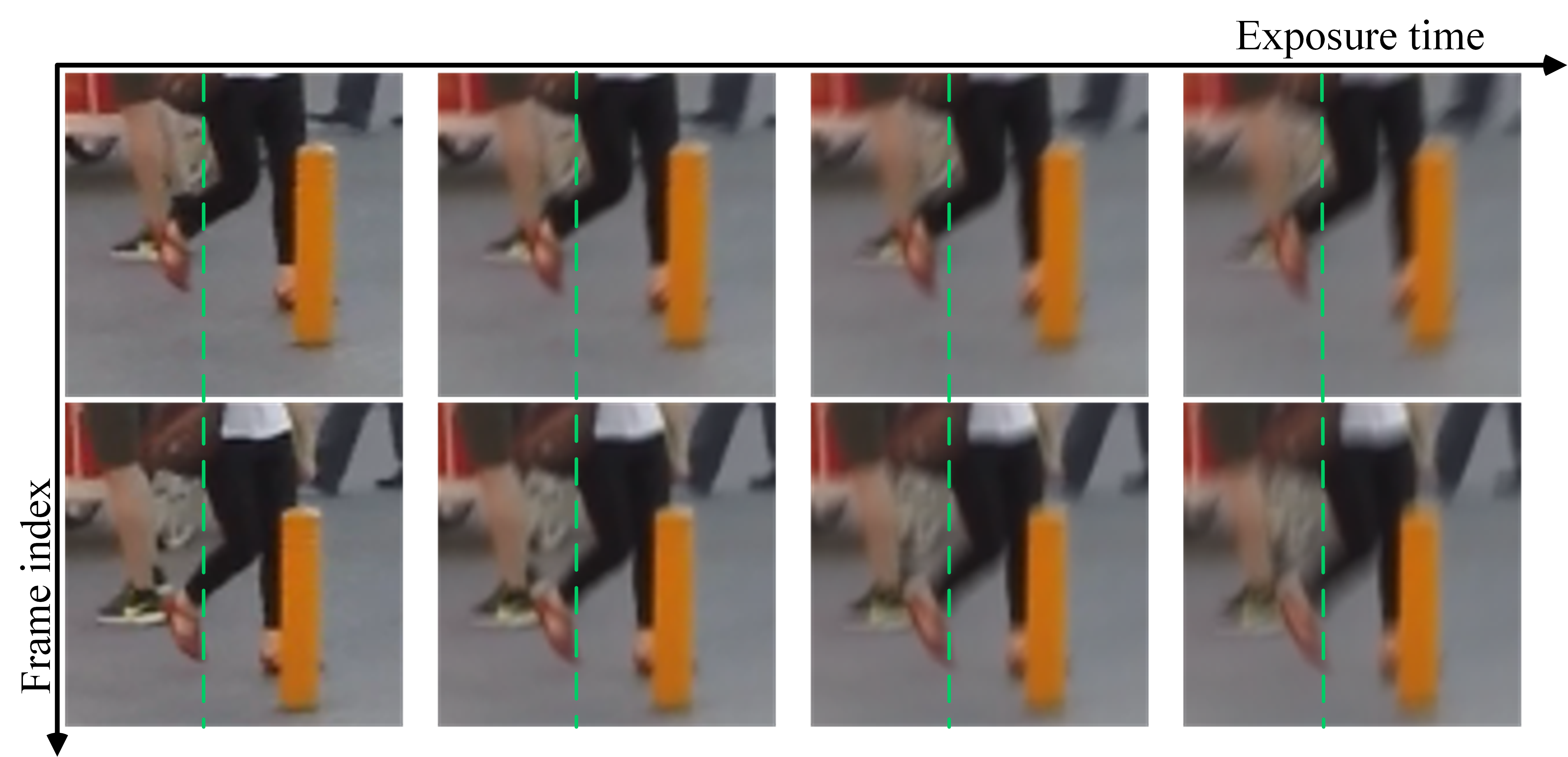
Figure 1: Visualization of motion blur under different exposure time and object motion. Frames from the left to right are obtained with increasing exposure time, leading to severer degree of motion blur. The situation may be worse if stronger motion is present, as illustrated by images in the second row.

1 Introduction

When capturing videos, shutter period (i.e., the inverse of the framerate) and exposure time are two major factors that we are able to manipulate for improved video quality, compared to other confounding factors such as object motion in the scene, lens imperfection, and sensor limitations [3]. Particularly, a long shutter period corresponds to lower framerate, and a longer exposure time increases the possibility of introducing severer motion blur (see Fig. 1). Often, we have good control over the shutter period in the form of the framerate, which is, nevertheless, quite limited in consumer cameras (e.g., $30$ frames per second, or FPS). This is not the case for exposure time, which may constantly and dynamically change depending on the video shooting environment, e.g., illumination and reflection conditions [25]. Therefore, video frame interpolation (also known as framerate up-conversion [5, 10, 15]) and video deblurring methods (under unknown exposure time) are crucial for improving the quality of low framerate blurred videos, and are widely applicable to video editing, video compression, and slow-motion video generation.

In literature, video frame interpolation [30, 21, 48, 42] and video deblurring [35, 9] have long been treated as individual problems and tackled separately with worth-celebrating successes. A straightforward approach to joint video frame interpolation and deblurring is to deploy deblurring methods followed by frame interpolation. However, this type of cascaded methods usually cannot obtain satisfactory reconstruction results, since algorithm-dependent deblurring artifacts would be propagated to and amplified in interpolated frames [41]. Similar situations will occur if we cascade video frame interpolation first [1]. This inspires recent work [34, 41, 1, 47] to cast video frame interpolation and deblurring (or super-resolution) as a joint and emerging low-level vision problem. However, these methods assume known and fixed exposure time in the video degradation model, which is unrealistic, especially when the auto-exposure mode is enabled. Thus, they are bound to generalize poorly in the real-world.

Currently, there are two studies [51, 25] considering the setting of unknown exposure time. Zhang et al. [51] computed generic quadratic motion trajectories from consecutive blurred (or estimated sharp) frames. They directly cascaded existing deblurring and frame interpolation methods, suffering from the error propagation problem. Benefiting from additional event cameras [4], Kim [25] proposed an event-guided and end-to-end optimized video deblurring method under unknown exposure time, but event sensors have not been equipped on consumer cameras, restricting its practical applications.

In this work, we aim ambitiously for the more realistic and challenging task - joint video multi-frame interpolation and deblurring under unknown exposure time. Our primary design philosophy is adaptive computation: we adapt our Video frame Interpolation and Deblurring method under Unknown Exposure time (VIDUE) to exposure-aware and motion-aware representations, where the computation of the motion-aware representation is further adapted to the exposure-aware representation. To achieve this, we first adopt a variant of supervised contrastive learning to extract an exposure-aware representation from a low framerate blurred video. We then train two U-Nets: one is responsible for intra-motion analysis (e.g., assessing motion complexity within each frame); the other is responsible for inter-motion analysis (e.g., assessing motion continuity between frames). We adapt the two U-Nets to the exposure-aware representation via gain tuning [31] (also can be seen as a variant of sequence-and-excitation [16]). We last develop a video reconstruction network with a U-Net-like structure, which enables exposure-adaptive convolution and motion refinement in a progressive fashion.

Extensive experiments on both synthetic and real datasets show that the proposed VIDUE consistently produces higher-quality deblurred and $\times 8$ interpolated frames both visually and in terms of standard quality metrics. Moreover, VIDUE exhibits significant performance gains ($\geq 1.5$ dB) over the state-of-the-art on the seemingly implausible $\times 16$ interpolation and deblurring task.

2 Related Work

2.1 Video Frame Interpolation

The video industry has long been interested in increasing the temporal resolution of a video sequence, i.e., framerate up conversion [7, 10, 18], with primary application to video compression. The problem resurges in the computer vision community under the name of video frame interpolation along with the renaissance of deep learning. Both Center-Frame Interpolation (CFI) [33, 11, 2, 30] and Multi-Frame Interpolation (MFI) [48, 17, 19] have been extensively investigated. For center-frame interpolation, Niklaus et al. [33] proposed separable kernel prediction networks to handle large motion, optimized by “perceptual” losses [20]. Bao et al. [2] proposed to incorporate depth information during interpolation to combat occlusion through bidirectional flow estimation. Lee et al. [30] combined and generalized the kernel-based and flow-based methods by offset prediction, and introduced an adversarial loss to examine the naturalness of the interpolated frame w.r.t. adjacent input frames. For multi-frame interpolation, more complex motion trajectory models need to be specified compared to the linear model assumption typically used in center-frame interpolation. Xu et al. [48] proposed a quadratic interpolation scheme to allow the inter-motion to be curvilinear. Chi et al. [8] proposed a cubic-based motion model with a relaxed warping loss to further boost interpolation accuracy for complex motion scenes. Huang et al. [17] designed the so-called privileged distillation scheme for real-time arbitrary timestamp frame interpolation. In addition, Kalluri et al. [21] cast multi-frame interpolation as a self-supervised pretext task to benefit downstream video applications, such as action recognition and video object tracking. 3D convolutions were adopted for spatiotemporal feature extraction. All these methods would encounter difficulties when processing motion-blurred videos because the optical flow/motion estimation as the core module will become less accurate.

2.2 Image and Video Deblurring

Traditionally, image deblurring is formulated as a Maximum A Posteriori (MAP) problem, which relies heavily on natural image priors, such as total variation [6], smoothness priors based on Markov random fields [37], normalized sparsity [28], and color-line priors [29]. Recent image deblurring methods adopt a pure data-driven approach, learning to deblur from massive deblurred-clean image pairs [49, 9]. Among popular architectural design choices, coarse-to-fine estimation has been extensively studied [12, 32, 36, 9]. For example, Chi et al. [9] adopted a U-Net to accept blurred images of multiple scales, and produce the corresponding set of sharp images in parallel. Alternatively, Ren et al. [38] proposed an unsupervised image deblurring scheme by leveraging deep priors [44] of both underlying sharp images and blur kernels. For video deblurring, the added temporal dimension can be coped with recurrent computation [14, 52], optical flow estimation [26, 35, 40], and deformable convolution [45], aided by handcrafted priors [35] or complementary modalities [40]. Image/video deblurring can only restore existing blurred frames, even motion information between input frames are computed to facilitate deblurring, which is kind of computational waste. Therefore, it is rational to consider joint video frame interpolation and deblurring, especially when the motion between consecutive frames is computed in either case.

2.3 Joint Video Interpolation and Deblurring

Recently, some researchers began to address the problem of joint video frame interpolation and deblurring. Shen et al. [41] proposed a pyramidal method for center-frame interpolation and deblurring. Argaw et al. [1] adopted a motion-based approach for not only multi-frame interpolation but also extrapolation. Oh et al. [34] introduced flow-guided attention and recursive feature refinement to improve the reconstruction performance. All these methods assume known and fixed exposure time, which is less realistic. Closest to ours, Zhang et al. [51] chose to cascade deblurring and interpolation networks under unknown exposure time. However, the performance would inevitably be compromised by the inaccuracy of the optical flow module in the deblurring network. Here, the proposed VIDUE is designed to adapt its computation to exposure-aware and motion-aware representations for joint video multi-frame interpolation and deblurring under unknown exposure time.

3 Proposed VIDUE

In this section, we first present the problem formulation of joint video frame interpolation and deblurring under unknown exposure time, and then describe in detail the proposed VIDUE method, consisting of an exposure-aware feature extractor $g_{e}$, an intra- and inter-motion analyzer $g_{a}$, and a video reconstruction network $f$.

3.1 Problem Formulation

When capturing a video frame, the shutter period $\Delta t$ includes two phases: the exposure phase $\Delta t_{e}$ and the effective readout phase $\Delta t_{r}$, where $\Delta t=\Delta t_{e}+\Delta t_{r}$. Given a video with $T$ frames $\bm{y}=\{\bm{y}_{t}\}_{t=1}^{T}$, the $t$-th frame $\bm{y}_{t}$ is essentially an integral of the latent image $\bm{x}_{\tau}$ at each instant time $\tau$ over the exposure time $\Delta t_{e}$:

$$\bm{y}_{t}=\frac{1}{\Delta t_{e}}{\int}_{\tau=t\cdot\Delta t}^{\tau=t\cdot\Delta t+\Delta t_{e}}\bm{x}_{\tau}d{\tau}.\\$$ (1)

For consumer-grade cameras, the captured videos for dynamic scenes usually suffer from low framerate and blur due to long shutter period with a large portion of exposure time. Joint video $\times S$ interpolation and deblurring aims to recover a high framerate video with sharp frames: $\bm{x}=\{\bm{x}_{t}\}_{t=1}^{T\times S}$ from the observed video $\bm{y}$. In this work, we assume the shutter period $\Delta t$ is known, while the exposure time $\Delta t_{e}$ is not, and thus $\Delta t_{e}$ is directly linked to the strength of the motion blur. It is noteworthy that the formulation in Eq. (1) is different from DeMFI [34], which synthesizes blur by directly averaging consecutive frames, while ignoring the readout phase.

3.2 Exposure-Aware Feature Extractor

Our first design choice is that the video reconstruction network $f$ should adapt to different exposure time. For the $\times S$ interpolation task, we have the same number of $S$ exposure time durations, where $\Delta t_{e}\in\{1,2,\ldots,S\}$ and $\Delta t=S$ in Eq. (1). $\Delta t_{e}:\Delta t=S:S$ means that the effective readout time $\Delta t_{r}$ is zero. That is, the actual readout phase is fully overlapped with the next exposure phase.

We work with a mini-batch of input video sequences, from which we create two multiviewed versions by applying horizontal and vertical flipping, 90° rotation, and random cropping to obtain $\mathcal{B}=\{(\bm{y}^{(i)},\Delta t_{e}^{(i)})\}_{i=1}^{|\mathcal{B}|}$ with $\bm{y}^{(i)}\in\mathbb{R}^{(T\times 3)\times H\times W}$. We combine the temporal and channel dimensions into one to naïvely enable spatiotemporal analysis using 2D convolutions. We adopt a variant of ResNet18 as $g_{e}:\mathbb{R}^{(T\times 3)\times H\times W}\mapsto\mathbb{R}^{C\times 1}$, where we replace the classification head with two Fully-Connected (FC) layers with leaky ReLU nonlinearity in between, to extract the exposure-aware feature representation $\bm{u}^{(i)}\in\mathbb{R}^{C\times 1}$.

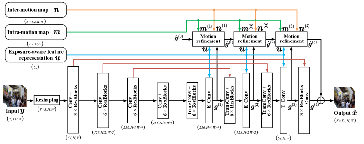
Figure 2: Overview of the reconstruction network of VIDUE, by which low framerate blurred video $\bm{y}$ with $T$ frames can be reconstructed to high framerate sharp video with $S\times T$ frames for the $\times S$ interpolation and deblurring task. The reconstruction network is built upon the exposure-aware representation $\bm{u}$ and motion-aware representations $\bm{m}$ and $\bm{n}$ by exposure-adaptive convolution, and we implement progressive motion refinement for better reconstruction performance.

We want to make the feature representations $\{\bm{u}^{(i)}\}$ corresponding to different exposure time to be as discriminative as possible. Thus we resort to supervised contrastive learning [24], and introduce the relative weighting to indicate the difference in exposure time between each sample and the anchor:

$$\small\ell_{\mathrm{ws}}=\sum_{\bm{u}\in\mathcal{B}}\frac{-1}{|\mathcal{P}|}\sum_{\bm{v}\in\mathcal{P}}\log\frac{\exp\left(\bm{u}^{\intercal}\bm{v}/\alpha\right)}{\sum\limits_{\bm{v}^{\prime}\in\mathcal{B}\setminus\{\bm{u}\}}{w}(\bm{u},\bm{v}^{\prime})\cdot\exp\left(\bm{u}^{\intercal}\bm{v}^{\prime}/\alpha\right)},$$ (2)

where $\bm{u}$ denotes the anchor, $\mathcal{P}$ contains positive samples that share the same exposure time with the anchor, and $\alpha$ is a fixed temperature parameter. The relative weighting can be straightforwardly computed by $w(\bm{u}^{(i)},\bm{u}^{(j)})=\left|\Delta t_{e}^{(i)}-\Delta t_{e}^{(j)}\right|$. We also try to formulate the exposure-aware feature representation learning as ordinal regression [13], but obtain worse final results (see Table 4). After training, the exposure-aware feature extractor $g_{e}$ is fixed during the training of the motion analyzer and the final reconstruction network.

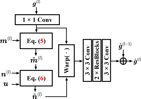
Figure 3: Overview of the proposed progressive motion refinement module. We first refine the intra-motion maps $\bm{m}^{(l)}$ with the help of $\bm{g}^{(l)}$ to obtain $\tilde{\bm{m}}^{(l)}$, and then refine the inter-motion maps $\bm{n}^{(l)}$ based on $\tilde{\bm{m}}^{(l)}$ and $\bm{u}$. Finally, we obtain the motion-refined output feature $\hat{\bm{g}}^{(l)}$ by warping the input feature $\bm{g}^{(l)}$ according to $\tilde{\bm{n}}^{(l)}$, followed by further refinement and incorporation of the upsampled $\hat{\bm{g}}^{(l-1)}$ from the previous stage via addition.

3.2.1 Intra- and Inter-Motion Analyzer

Our second design choice is that the video reconstruction network $f$ should adapt to different motion patterns presented in dynamic scenes. We choose to analyze both intra-motion within each video frame, which is relevant to motion complexity (captured in a given exposure time period $\Delta t_{e}$), and inter-motion between frames, which is pertinent to motion continuity (captured in a given shutter period $\Delta t$). Our motion analyzer $g_{a}:\mathbb{R}^{(T\times 3)\times H\times W}\mapsto\mathbb{R}^{T\times 1\times H\times W}\times\mathbb{R}^{(S\times T)\times 2\times H\times W}$, computes, from an input video sequence $\bm{y}^{(i)}$, $T$ intra-motion maps and $S\times T$ inter-motion maps of the same spatial size, respectively, whose computation is adaptive to the exposure-aware representation $\bm{u}^{(i)}$.

Intra-Motion Analysis. We adopt a pre-trained light-weight U-Net [50], in which we tune the “gain” (i.e., a single multiplicative scaling parameter) of each channel of the intermediate representations $\bm{z}\in\mathbb{R}^{C^{\prime}\times H^{\prime}\times W^{\prime}}$ (in the expansive path [39]):

$$\bm{g}_{i\bullet}=\bm{u}^{\prime}_{i}\cdot\bm{z}_{i\bullet},\quad\bm{u}^{\prime}=\sigma\left(\mathbf{W}_{2}^{\intercal}\mathrm{LReLU}\left(\mathbf{W}_{1}^{\intercal}\bm{u}\right)\right).$$ (3)

Here $\bm{z}_{i\bullet}$ stands for the $i$-th channel, and $\bm{u}^{\prime}\in\mathbb{R}^{C^{\prime}\times 1}$ is the gain vector computed from the exposure-aware representation $\bm{u}$ by two FC layers with leaky ReLU in between, followed by a Sigmoid function $\sigma(\cdot)$. $\{\mathbf{W}_{1},\mathbf{W}_{2}\}$ are learnable weight matrices. Eq. (3) can also be seen as a form of the squeeze-and-excitation operation [16], where we “squeeze” the raw video sequence into $\bm{u}^{\prime}$ through $\bm{u}$, and use it to “excite” $\bm{z}$. The results from the U-Net are intra-motion offsets $\bm{o}^{(s)}\in\mathbb{R}^{T\times 2\times H\times W}$ and $\bm{o}^{(e)}\in\mathbb{R}^{T\times 2\times H\times W}$, which are the starting and ending positions of estimated motion trajectories in horizontal and vertical directions, respectively. We compute the final intra-motion maps $\bm{m}\in\mathbb{R}^{T\times 1\times H\times W}$ by subtracting $\bm{o}^{(e)}$ from $\bm{o}^{(s)}$, followed by root mean squared of the subtracted offsets. Intra-motion maps can also be integrated into $g_{e}$ to improve representation capabilities.

Method	Inference time (sec)	GoPro-5:8			GoPro-7:8
	/ Framerate (FPS)	Deblurring	Interpolation	Avg	Deblurring	Interpolation	Avg
CDVD-TSP+QVI	1.02 / 7.84	33.06 / 0.952	30.02 / 0.914	30.40 / 0.918	31.39 / 0.933	29.39 / 0.902	29.64 / 0.906
CDVD-TSP+RIFE	0.40 / 20.00		29.95 / 0.907	30.34 / 0.913		29.15 / 0.892	29.44 / 0.897
MIMOUNetPlus+QVI	0.78 / 10.26	34.42 / 0.961	30.48 / 0.920	30.97 / 0.925	33.15 / 0.951	30.18 / 0.915	30.55 / 0.920
MIMOUNetPlus+RIFE	0.16 / 50.00		30.83 / 0.921	31.28 / 0.926		30.33 / 0.913	30.69 / 0.918
UTI-VFI	0.68 / 11.76	—	—	34.40 / 0.965	—	—	33.28 / 0.955
FLAVR	0.50 / 16.00	35.78 / 0.968	34.20 / 0.959	34.39 / 0.960	33.72 / 0.953	33.36 / 0.952	33.41 / 0.952
DeMFI	3.19 / 2.51	36.69 / 0.974	34.77 / 0.965	35.01 / 0.967	35.01 / 0.964	34.43 / 0.962	34.50 / 0.962
VIDUE (Ours)	0.27 / 29.63	37.74 / 0.980	36.12 / 0.973	36.32 / 0.974	36.12 / 0.973	35.56 / 0.970	35.63 / 0.970

Table 1: PSNR / SSIM comparison results on the GoPro dataset. “Deblurring” and “Interpolation” columns contain the reconstruction results of the input and interpolated frames, respectively, while the “Avg” column summarizes the average performance.

TSP + QVI	TSP + RIFE	MIMO + QVI	MIMO + RIFE	UTI-VFI	FLAVR	DeMFI	VIDUE (Ours)	GT

Figure 4: Visual comparison on the GoPro dataset. Orange and green boxes indicate cropped patches for zoomed-in comparison from deblurred and interpolated frames, respectively. TSP and MIMO are short for CDVD-TSP and MIMOUNetPlus, respectively. GT stands for the ground-truth patches cropped from the reference high framerate video.

Inter-Motion Analysis. We adopt a second randomly initialized light-weight U-Net, taking the estimated intra-motion offsets $\bm{o}^{(s)}$ and $\bm{o}^{(e)}$ as inputs, and producing inter-motion maps $\bm{n}\in\mathbb{R}^{(S\times T)\times 2\times H\times W}$. The adaptive gain tuning in Eq. (3) is also enabled in the expansive path of the U-Net. The detailed network specifications of the motion analyzer can be found in the supplementary.

3.3 Video Reconstruction Network

It is then ready to describe our video reconstruction network $f:\mathbb{R}^{T\times 3\times H\times W}\mapsto\mathbb{R}^{(S\times T)\times 3\times H\times W}$, which is built upon the exposure-aware representation $\bm{u}$ and the motion-aware representations $\bm{m}$ and $\bm{n}$ by progressive exposure-adaptive convolution and motion refinement. The architecture is shown in Fig. 2.

We first feed the input video sequence $\bm{y}\in\mathbb{R}^{(T\times 3)\times H\times W}$ into an encoder, which consists of four stages of residual blocks, separated by the spatially downsampling layers. Each residual block contains two $3\times 3$ convolution layers with leaky ReLU in between. Similarly, the decoder is composed of three stages of one transposed convolution for upsampling, residual blocks, one exposure-adaptive convolution, and one motion refinement module, followed by a back-end residual block and a convolution layer for channel number adjustment.

Exposure-Adaptive Convolution. Motivated by [22, 23], we propose to further convolve the intermediate representation $\bm{z}$ from the residual blocks using a filter bank, in which we adapt the filter weights to the exposure-aware representation $\bm{u}$. We generate the filter weights $\bm{w}$ by

$$\bm{u}^{\prime} =\mathbf{W}_{2}^{\intercal}\mathrm{LReLU}\left(\mathbf{W}_{1}^{\intercal}\bm{u}\right),$$ (4)

$$\bm{w}_{ijk} =\frac{\bm{w}^{\prime}_{ijk}\cdot\bm{u}^{\prime}_{i}}{\sqrt{\sum_{i,k}(\bm{w}^{\prime}_{ijk}\cdot\bm{u}^{\prime}_{i})^{2}+\epsilon}},$$

where $\{\bm{w}^{\prime},\mathbf{W}_{1},\mathbf{W}_{2}\}$ are learnable, and $i$, $j$, and $k$ index the input feature channel, the output feature channel, and the spatial footprint of the convolution, respectively. $\epsilon$ is a small positive constant to avoid numerical instability issues. As in [23], we first perform instance normalization of the feature representation $\bm{z}$ with the learnable scaling factor and the bias term, followed by the exposure-adaptive convolution to obtain $\bm{g}$ (refer to the notations in Fig. 2).

Motion Refinement Module. At the $l$-th stage for $l\in\{1,2,3\}$, the motion refinement module accepts $\bm{g}^{(l)}$ from the exposure-adaptive convolution as input, whose channel dimension is adjusted by a $1\times 1$ convolution. The intra-motion maps $\bm{m}$ and the inter-motion maps $\bm{n}$ are accordingly resized to the same spatial size with $\bm{g}^{(l)}$, denoted by $\bm{m}^{(l)}$ and $\bm{n}^{(l)}$, respectively. We refine the intra-motion maps by

$$\tilde{\bm{m}}^{(l)}=\sigma\left(\mathrm{Conv}\left(\mathrm{Concat}\left(\bm{m}^{(l)},\bm{g}^{(l)}\right)\right)+\bm{m}^{(l)}\right),$$ (5)

where $\mathrm{Conv}(\cdot)$ denotes a $3\times 3$ convolution, $\mathrm{Concat}(\cdot)$ denotes the concatenation operation along the channel dimension, and $+$ indicates that we rely on a residual connection for implementation. We continue to refine the inter-motion maps $\bm{n}^{(l)}$ based on $\tilde{\bm{m}}^{(l)}$:

$$\tilde{\bm{n}}^{(l)}\!\!=\mathrm{Conv}(\mathrm{E\_Conv}(\bm{n}^{(l)}\!\!,\bm{u})\odot\tilde{\bm{m}}^{(l)}\!\!+\!\bm{n}^{(l)}\odot(1\!-\!\tilde{\bm{m}}^{(l)})),$$ (6)

where $\mathrm{E\_Conv(\cdot)}$ stands for the exposure-adaptive convolution and $\odot$ is an element-wise multiplication operation.

Progressive Reconstruction. Finally, we make use of the refined inter-motion maps $\tilde{\bm{n}}^{(l)}$ and the input features $\bm{g}^{(l)}$ for progressive reconstruction:

$$\hat{\bm{g}}^{(l)}=\mathrm{Refine}(\mathrm{Warp}(\bm{g}^{(l)},\tilde{\bm{n}}^{(l)}))+\mathrm{Up}(\hat{\bm{g}}^{(l-1)}),$$ (7)

where $\mathrm{Warp}(\cdot)$ denotes the backward warping function [35], and $\mathrm{Up}(\cdot)$ denotes the bilinear upsampling operation. $\mathrm{Refine}(\cdot)$ is implemented by a front-end convolution layer, two residual blocks, and a back-end convolution layer. To initialize progressive reconstruction, we set $\hat{\bm{g}}^{(0)}=\bm{0}$ as a tensor with all zeros, and summarize one stage of processing in Fig. 3. At last, we add $\bm{g}^{(4)}$ (i.e., the output of the back-end residual block and convolution layer in the decoder) to $\hat{\bm{g}}^{(3)}$ to estimate the high framerate sharp video sequence $\hat{\bm{x}}\in\mathbb{R}^{(S\times T)\times 3\times H\times W}$.

During training, we optimize all modules in the proposed VIDUE method (except for the exposure-aware feature extractor) using a variant of stochastic gradient descent by minimizing the Mean Absolute Error (MAE) between the ground-truth high framerate sharp video sequences and their predictions by VIDUE.

Method	Adobe-5:8			Adobe-7:8
	Deblurring	Interpolation	Avg	Deblurring	Interpolation	Avg
CDVD-TSP+QVI	29.34 / 0.896	23.34 / 0.739	24.10 / 0.759	27.57 / 0.862	23.42 / 0.741	23.94 / 0.756
CDVD-TSP+RIFE		23.29 / 0.729	24.06 / 0.750		23.31 / 0.730	23.85 / 0.747
MIMOUNetPlus+QVI	29.71 / 0.894	23.48 / 0.741	24.27 / 0.761	27.69 / 0.854	23.52 / 0.740	24.05 / 0.754
MIMOUNetPlus+RIFE		23.85 / 0.748	24.59 / 0.767		23.76 / 0.744	24.26 / 0.758
UTI-VFI	—	—	26.69 / 0.842	—	—	25.84 / 0.815
FLAVR	28.52 / 0.869	27.05 / 0.841	27.23 / 0.845	26.98 / 0.834	26.94 / 0.837	26.94 / 0.837
DeMFI	27.24 / 0.848	25.49 / 0.814	25.71 / 0.818	25.81 / 0.813	25.64 / 0.814	25.66 / 0.814
VIDUE (Ours)	30.44 / 0.905	28.50 / 0.876	28.74 / 0.880	27.85 / 0.864	27.92 / 0.867	27.91 / 0.866

Table 2: PSNR / SSIM comparison results on the Adobe dataset.

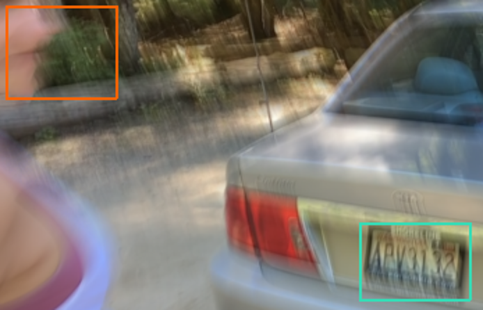
Blurred Frame

TSP + QVI	TSP + RIFE	MIMO + QVI	MIMO + RIFE	UTI-VFI	FLAVR	DeMFI	VIDUE (Ours)	GT

Figure 5: Visual comparison on the Adobe dataset. Orange and green patches are from deblurred and interpolated frames, respectively.

4 Experiments

In this section, we evaluate VIDUE on both synthetic and real-world datasets. More results including reconstructed videos can be found in the supplementary. The source code is implemented in Pytorch, and is made publicly available at https://github.com/shangwei5/VIDUE. We also provide an implementation in HUAWEI Mindspore at https://github.com/Hunter-Will/VIDUE-mindspore.

4.1 Datasets

To establish simulated datasets for quantitative performance comparison of video interpolation and deblurring, we synthesize low framerate videos according to Eq. (1) by downsampling high framerate videos [34, 51]. The experiments are conducted on both the GoPro dataset [32] and the Adobe dataset [43]. On the GoPro dataset with $\times 8$ interpolation (and deblurring) task, we set $S=8$ by which an original 240 FPS video is degraded to 30 FPS. For a fair comparison, we set exposure frames to two odd numbers, i.e., $\Delta t_{e}:\Delta t\in\{5:8,7:8\}$, since existing methods require the middle frame as reference. As for training, we sample $\Delta t_{e}:\Delta t\in\{1:8,2:8,\ldots,8:8\}$ to generate blurred frames as a form of data augmentation to train the exposure-aware feature extractor $g_{e}$. On the Adobe dataset with $\times 8$ interpolation (and deblurring) task, the synthetic setting is identical, but the blurring artifacts are more severe by setting a longer shutter period. Furthermore, we evaluate the generalizability of VIDUE against competing methods on real-world data from the RealBlur dataset [43].

Method	GoPro-9:16	GoPro-11:16	GoPro-13:16	GoPro-15:16	Avg
CDVD-TSP+QVI	25.70 / 0.786	25.45 / 0.780	25.20 / 0.774	24.97 / 0.767	25.33 / 0.777
CDVD-TSP+RIFE	26.08 / 0.797	25.74 / 0.788	25.41 / 0.780	25.12 / 0.772	25.59 / 0.784
MIMOUNetPlus+QVI	26.12 / 0.794	25.97 / 0.791	25.78 / 0.787	25.49 / 0.780	25.84 / 0.788
MIMOUNetPlus+RIFE	26.95 / 0.821	26.71 / 0.815	26.41 / 0.808	25.98 / 0.797	26.51 / 0.810
UTI-VFI	28.59 / 0.876	28.17 / 0.866	27.40 / 0.845	26.37 / 0.814	27.63 / 0.851
FLAVR	28.77 / 0.875	28.71 / 0.875	28.43 / 0.870	28.04 / 0.860	28.49 / 0.870
DeMFI	28.64 / 0.876	28.67 / 0.878	28.49 / 0.873	28.11 / 0.863	28.48 / 0.873
VIDUE (Ours)	31.10 / 0.922	29.91 / 0.906	29.90 / 0.905	29.50 / 0.898	30.10 / 0.908

Table 3: PSNR / SSIM comparison results on the GoPro dataset for joint $\times 16$ interpolation and deblurring.

Setting	GoPro-5:8	GoPro-7:8
Exposure-Agnostic	34.79 / 0.965	34.13 / 0.960
Ordinal Regression	35.44 / 0.969	34.97 / 0.966
Contrastive Learning	36.32 / 0.974	35.63 / 0.970
Known Exposure Time	36.41 / 0.974	35.87 / 0.971

Table 4: Role of the exposure-aware feature representation $\bm{u}$ evaluated by PSNR / SSIM. The default setting is highlighted in bold.

Exposure Representation		Intra-	Inter-	Motion	GoPro-5:8	GoPro-7:8
Squeeze-and-Excitation	$\mathrm{E\_Conv}$	Motion	Motion	Refinement
✗	✗	✗	✗	✗	34.79 / 0.965	34.13 / 0.960
✗	✓	✗	✗	✗	36.05 / 0.972	34.87 / 0.963
✗	✓	✗	✓	✗	36.18 / 0.973	35.27 / 0.968
✗	✓	✓	✗	✓	36.20 / 0.973	35.24 / 0.968
✗	✓	✓	✓	✗	36.23 / 0.974	35.28 / 0.968
✓	✗	✓	✓	✓	36.12 / 0.973	35.39 / 0.969
✗	✓	✓	✓	✓	36.32 / 0.974	35.63 / 0.970

Table 5: Module analysis of VIDUE on the GoPro dataset.

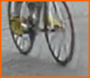
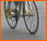
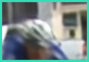
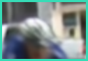
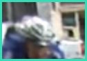
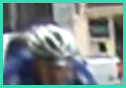
TSP + QVI	TSP + RIFE	MIMO + QVI	MIMO + RIFE	UTI-VFI	FLAVR	DeMFI	VIDUE (Ours)

Figure 6: Visual comparison on the RealBlur dataset. Orange and green patches are from deblurred and interpolated frames, respectively.

4.2 Implementation Details

We set the input frame number $T=4$, and the the exposure-aware feature dimension $C=256$. The temperature parameter in Eq. (2) and the normalizing constant in Eq. (4) is set to $\alpha=0.5$ and $\epsilon=1\times 10^{-5}$, respectively. We adopt the Adam [27] optimizer with the default setting for training $g_{e}$ with an initial learning rate of $0.1$ and a mini-batch size of $40$. Similarly, we adopt the AdaMax [27] optimizer with parameters $\beta_{1}=0.9$ and $\beta_{2}=0.999$ for training $g_{a}$ and $f$, and set the initial learning rate and the mini-batch size to $2\times 10^{-4}$ and $12$, respectively. We train the models for $200$ epochs, and halve the learning rate whenever the training plateaus, which is cross-validated as done in [21]. VIDUE is trained on $4$ Tesla V100 GPUs, and can make inference on a single GTX 2080 Ti GPU. Throughout the paper, we use the Peak Signal-to-Noise Ratio (PSNR) and the Structural SIMilarity (SSIM) index [46] as the evaluation metrics.

4.3 Evaluation on $\times 8$ Interpolation Task

We compare VIDUE with both cascade and joint methods. For cascade methods, deblurring methods CDVD-TSP [35], MIMOUNetPlus [9] and interpolation methods QVI [48], RIFE [17] are cascaded for video deblurring and interpolation. We also take UTI-VFI [51] into comparison, which handles unknown exposure time. For joint methods, we include FLAVR [21] and DeMFI [34]. It is worth noting that the original FLAVR is an interpolation method with sharp inputs, and we retrain it on the same training sets to tackle joint video interpolation and deblurring. For MIMOUNetPlus and RIFE, we find that models provided by the respective authors perform better than our retrained counterparts, and thus we stick to the official implementations for evaluation.

4.3.1 Comparison on the GoPro Dataset

As mentioned previously, we create two versions of the GoPro dataset, “GoPro-5:8” and “GoPro-7:8”, with different exposure time, and list the comparison results in Table 1. We find that cascade methods are significantly worse than joint methods, with a PSNR gap of almost $3$ to $6$ dB. In comparison with joint methods, VIDUE achieves about $1.0$ to $1.1$ dB PSNR gains for deblurring, and about $1.1$ to $1.4$ dB PSNR gains for interpolation, respectively. In terms of visual comparison in Fig. 4, cascade methods fail in interpolating sharp frames. The deblurring results of the joint methods FLAVR and DeMFI are satisfactory, but they are still limited in interpolation. This is because the unknown exposure time setting is not carefully modeled, and latent sharp frames during the readout phase cannot be properly reconstructed. In stark contrast, VIDUE is able to adapt to different exposure time based on the learned exposure-aware feature representation, and achieves noticeable performance gains on this challenging task of joint video multi-frame interpolation and deblurring. In addition, we test the inference time (and framerate) of all methods on the GoPro dataset. We calculate the average running time of reconstructing $8$ frames (i.e., using $\times 8$ interpolation as the example) on the Tesla V100 GPU. We find from Table 1 that VIDUE shows clear advantages over all competing methods except for the light-weight cascade method (i.e., MIMOUNetPlus+RIFE, which does not deliver convincing reconstruction performance). DeMFI involves extensive recurrent computation, leading to the longest inference time among all methods. In summary, the proposed VIDUE enjoys faster inference time, and achieves the best reconstruction performance, which justifies our key design philosophy of adaptive computation to deblurring and interpolation relevant features.

4.3.2 Comparison on the Adobe Dataset

We evaluate the joint $\times 8$ interpolation and deblurring performance of VIDUE against the competing methods in Table 2 and Fig. 5. Despite more severe blurring artifacts than those in the GoPro dataset, we come to similar conclusions that joint methods are superior over cascade methods. The most competitive method - DeMFI - experiences a significant performance drop due to the presence of the heavy blur. VIDUE still outperforms FLAVR about $0.9$ to $1.9$ dB for deblurring, and about $1.0$ to $1.4$ dB for interpolation, respectively. From Fig. 5, one can see that the competing methods fail to restore sharp frames, while VIDUE still obtains visually favorable results even in the presence of the strong blur.

4.3.3 Generalization to Real-World Videos

Finally, we evaluate the generalizability of VIDUE on real-world blurred frames by testing the model trained on the GoPro dataset to interpolate and deblur video data from the RealBlur dataset. As shown in Fig. 6, VIDUE achieves the most visually plausible interpolation and deblurring results with sharper structures and textures, while others suffer from visually annoying artifacts.

4.4 Evaluation on $\times 16$ Interpolation Task

Without auxiliary information (e.g., event signals [25]), joint $\times 16$ interpolation and deblurring is extremely difficult, and is rarely evaluated in literature. We conduct this experiment on the GoPro dataset, and list the results in Table 3. VIDUE achieves more than $1.5$ dB gains than existing methods, and performs consistently better under all exposure time settings, which are unknown. More visual comparisons are provided in the supplementary.

4.5 Ablation Studies

4.5.1 Effectiveness of Exposure-Aware Representation

As shown in Table 4, four VIDUE variants are trained on the GoPro dataset to verify the effectiveness of the exposure-aware feature representation $\bm{u}$: 1) one that is exposure-agnostic (i.e., without learning and adapting to $\bm{u}$), 2) one that learns $\bm{u}$ using ordinal regression, 3) one that learns $\bm{u}$ using supervised contrastive learning combined with relative weighting (as the default setting), 4) one with the known exposure time (as a form of upper bound). To leverage the known exposure time, we first represent it as an $S$-dimensional vector with the first $\Delta t_{e}$ entries being one and the remaining entries being zero. We then use two FC layers with leaky ReLU in between to map it into a $C$-dimensional feature representation, which can be readily adapted in VIDUE. As reported in Table 4, both exposure-aware feature representations learned by ordinal regression and supervised contrastive learning bring significant improvements than the exposure-agnostic variant. Compared to ordinal regression, our default choice of supervised contrastive learning is able to approach the “upper bound” with the known exposure time. We believe this arises because contrastive learning provides a more direct way of encouraging discriminative feature learning than ordinal regression learns to rank different exposure time.

4.5.2 Module Analysis

We single out the contribution of each component of VIDUE using the GoPro dataset. The first row in Table 5 shows the results of a plain U-Net, while the second row is obtained by a simplified VIDUE without motion analysis and adaptation in the decoder. Surprisingly, the simplified VIDUE achieves better results than existing methods, (see Tables 1 and 5). The performance gains by VIDUE is mostly attributed to the use of the exposure-aware representation by contrasting it to the plain U-Net. We next remove each component of VIDUE to verify its necessity. Most importantly, removing motion refinement leads to performance drops under different exposure time, especially when the exposure time is large (i.e., when the motion is strong). We also replace the exposure-adaptive convolution (i.e., $\mathrm{E\_Conv}$ defined in Eq. (4)) with the sequence-and-excitation operation [16], and find that $\mathrm{E\_Conv}$ is more effective in leveraging the exposure-aware representation. As expected, the full VIDUE achieves the best interpolation and deblurring performance.

5 Conclusion

We have described a computational method - VIDUE - for joint video multi-frame interpolation and deblurring under unknown exposure time. We trained contrastively to extract exposure-aware feature representation, which can then be embedded into intra- and inter-motion analyzer and the video reconstruction network via gain tuning and exposure-adaptive convolution, respectively. We refined the estimated motion representations for better progressive video reconstruction. We demonstrated the superiority of VIDUE on both synthetic and real-world datasets to perform $\times 8$ and $\times 16$ interpolation and deblurring tasks. Future work can be planed to 1) further reduce the computational complexity of VIDUE while retaining (or improving) the performance and 2) to optimize VIDUE by perceptual quality metrics with emphasis on temporal coherence.

Appendix A Network Architecture

As mentioned in the main manuscript, the proposed VIDUE consists of an exposure-aware feature extractor $g_{e}$, an intra- and inter-motion analyzer $g_{a}$, and a video reconstruction network $f$.

A.1 Exposure-Aware Feature Extractor

We illustrate the network structure of the exposure-aware feature extractor $g_{e}$ in Table S1, in which $\mathrm{ResBlock}$ is detailed in Table S2.

A.2 Intra- and Inter-Motion Analyzer

We choose to analyze both intra-motion within each video frame and inter-motion between frames. Our motion analyzer $g_{a}:\mathbb{R}^{(T\times 3)\times H\times W}\mapsto\mathbb{R}^{T\times 1\times H\times W}\times\mathbb{R}^{(S\times T)\times 2\times H\times W}$, computes, from an input video sequence, $T$ intra-motion maps and $(S\times T)\times 2$ inter-motion maps of the same size, respectively. We show the network structure for intra-motion analysis in Table S3. The network structure for inter-motion analysis is similar to RefineNet proposed in [48], which is detailed in Table S4.

A.3 Video Reconstruction Network

The video reconstruction network $f:\mathbb{R}^{T\times 3\times H\times W}\mapsto\mathbb{R}^{(S\times T)\times 3\times H\times W}$ is built upon the exposure-aware representation $\bm{u}$ and motion-aware representations $\bm{m}$ and $\bm{n}$ by progressive exposure-adaptive convolution and motion refinement. The network structure is illustrated in Table S5.

Appendix B More Results on Benchmark Datasets

In this section, we provide more visual results of VIDUE in comparison to existing video interpolation and deblurring methods. Please refer to the link for more visual results at https://onedrive.live.com.

B.1 More Results on the GoPro Dataset

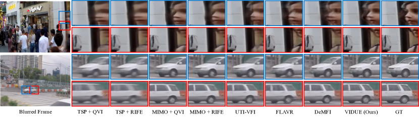
Figure S1: More visual results on GoPro [32] ($\times 8$). Blue and red patches are from deblurred and interpolated frames, respectively. TSP is short for CDVD-TSP, and MIMO is short for MIMOUNetPlus.

On the GoPro dataset with mild blur, VIDUE generally achieves more visually appealing results with sharper boundaries and fewer artifacts, as shown in Figs. S1 and S2.

B.2 More Results on the Adobe Dataset

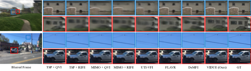
Figure S3: More visual results on Adobe [43] ($\times 8$). Blue and red patches are from deblurred and interpolated frames, respectively.

On the Adobe dataset with heavy blur, VIDUE still performs favorably as shown in Figs. S3 and S4.

B.3 More Results on the RealBlur Dataset

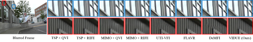
Figure S5: More visual results on RealBlur [43] ($\times 8$). Blue and red patches are from deblurred and interpolated frames, respectively.

On the RealBlur dataset, VIDUE generates the least artifacts and sharper textures compared with other methods, as shown in Figs. S5 and S6.

B.4 More Results on Video $\times 16$ Interpolation and Deblurring

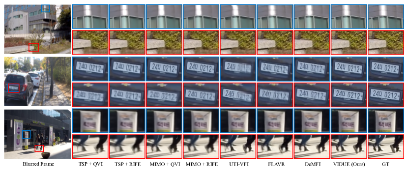
Figure S7: More visual results on GoPro [32] ($\times 16$). Blue and red patches are from deblurred and interpolated frames, respectively.

Although video $\times 16$ interpolation and deblurring is extremely difficult (without the help of extra auxiliary information), VIDUE is better at it than others, as shown in Figs. S7 and S8.

	Input	A sequence of blurred frames ($\mathrm{indim}=T\times 3$)
	Layer 1	$\mathrm{Conv}(\mathrm{indim},64,7,1,3);\mathrm{BN};\mathrm{LeakyReLU};\mathrm{ResBlock}(64,64,3,1,1,\mathrm{BN=True})\times 2$
	Layer 2	$\mathrm{Conv}(64,128,3,2,1);\mathrm{BN};\mathrm{LeakyReLU};\mathrm{ResBlock}(128,128,3,1,1,\mathrm{BN=True})\times 2$
	Layer 3	$\mathrm{Conv}(128,256,3,2,1);\mathrm{BN};\mathrm{LeakyReLU};\mathrm{ResBlock}(256,256,3,1,1,\mathrm{BN=True})\times 2$
	Layer 4	$\mathrm{Conv}(256,256,3,2,1);\mathrm{BN};\mathrm{LeakyReLU};\mathrm{ResBlock}(256,256,3,1,1,\mathrm{BN=True})\times 2$
	Layer 5	$\mathrm{GlobalAvgPool}$
	Layer 6	$\mathrm{Linear}(256,1024);\mathrm{LeakyReLU};\mathrm{Linear}(1024,256)$
	Output	Exposure-aware feature representation $\bm{u}$

Table S1: The structure of the exposure-aware feature extractor $g_{e}$. $T$ is the length of the input video sequence. $\mathrm{BN}$ stands for batch normalization. Convolution is in the form of (input  channel, output  channel, kernel  size, stride, padding). The linear (i.e., fully-connected) layer is in the form of (input  channel, output  channel).

	Layer 1	$\mathrm{Conv}(D,D,3,1,1);\mathrm{BN};\mathrm{LeakyReLU}$
	Layer 2	$\mathrm{Conv}(D,D,3,1,1);\mathrm{BN}$
		Residual connection between the input and the output of Layer 2 via addition

Table S2: The structure of $\mathrm{ResBlock}$. We may remove $\mathrm{BN}$ by setting the corresponding indicator variable to $\mathrm{False}$. $D$ is the channel dimension of the feature maps from the previous layer.

	Input	One blurred frame ($\mathrm{indim}=3$)
	Layer 1	$\mathrm{PixelUnshuffle}(2)$
	Layer 2	$\mathrm{Conv}(\mathrm{indim}\times 4,16,5,1,2);\mathrm{ResBlock}(16,16,5,1,2,\mathrm{BN}=\mathrm{False})\times 3$
	Layer 3	$\mathrm{Conv}(16,32,5,2,(1,2,1,2));\mathrm{ResBlock}(32,32,5,1,2,\mathrm{BN}=\mathrm{False})\times 3$
	Layer 4	$\mathrm{Conv}(32,64,5,2,(1,2,1,2));\mathrm{ResBlock}(64,64,5,1,2,\mathrm{BN}=\mathrm{False})\times 3$
	Layer 5	$\mathrm{Conv}(64,128,1,1,0);\mathrm{LeakyReLU};\mathrm{Conv}(128,64,3,1,1);\mathrm{LeakyReLU}$
	Layer 6	$\mathrm{SE}(256,64,4);\mathrm{TransConv}(64,32,4,2,1);\mathrm{LeakyReLU}$
		Concatenation of outputs from Layer 6 and Layer 3
	Layer 7	$\mathrm{Conv}(64,128,1,1,0);\mathrm{LeakyReLU};\mathrm{Conv}(128,64,3,1,1);\mathrm{LeakyReLU}$
	Layer 8	$\mathrm{SE}(256,64,4);\mathrm{TransConv}(64,16,4,2,1);\mathrm{LeakyReLU}$
		Concatenation of outputs from Layer 8 and Layer 2
	Layer 9	$\mathrm{Conv}(32,64,1,1,0);\mathrm{LeakyReLU};\mathrm{Conv}(64,32,3,1,1);\mathrm{LeakyReLU}$
	Layer 10	$\mathrm{SE}(256,32,4);\mathrm{TransConv}(32,32,4,2,1);\mathrm{LeakyReLU}$
	Layer 11	$\mathrm{Conv}(32,4,5,1,2)$
	Output	Motion offsets

Table S3: The structure of intra-motion analysis. Adapting to $\bm{u}$ via gain tuning is in the form of squeeze-and-excitation ($\mathrm{SE}$) (vec  channel, input  channel, reduction). Transposed convolution is in the same format as convolution.

	Input	A sequence of motion offsets ($\mathrm{indim}=T\times 4$)
	Layer 1	$\mathrm{Conv}(\mathrm{indim},32,7,1,3);\mathrm{LeakyReLU};\mathrm{Conv}(32,32,7,1,3);\mathrm{LeakyReLU}$
	Layer 2	$\mathrm{AvgPool}(2);\mathrm{Conv}(32,64,5,1,2);\mathrm{LeakyReLU};\mathrm{Conv}(64,64,5,1,2);\mathrm{LeakyReLU}$
	Layer 3	$\mathrm{AvgPool}(2);\mathrm{Conv}(64,128,3,1,1);\mathrm{LeakyReLU};\mathrm{Conv}(128,128,3,1,1);\mathrm{LeakyReLU}$
	Layer 4	$\mathrm{AvgPool}(2);\mathrm{Conv}(128,256,3,1,1);\mathrm{LeakyReLU};\mathrm{Conv}(256,256,3,1,1);\mathrm{LeakyReLU}$
	Layer 5	$\mathrm{AvgPool}(2);\mathrm{Conv}(256,512,3,1,1);\mathrm{LeakyReLU};\mathrm{Conv}(512,512,3,1,1);\mathrm{LeakyReLU}$
	Layer 6	$\mathrm{AvgPool}(2);\mathrm{Conv}(512,512,3,1,1);\mathrm{LeakyReLU};\mathrm{Conv}(512,512,3,1,1);\mathrm{LeakyReLU}$
	Layer 7	$\mathrm{Up}(2);\mathrm{Conv}(512,512,3,1,1);\mathrm{LeakyReLU};\mathrm{Conv}(512,512,3,1,1);\mathrm{LeakyReLU};\mathrm{SE}(256,512,4)$
	Layer 8	$\mathrm{Up}(2);\mathrm{Conv}(512,256,3,1,1);\mathrm{LeakyReLU};\mathrm{Conv}(256,256,3,1,1);\mathrm{LeakyReLU};\mathrm{SE}(256,256,4)$
	Layer 9	$\mathrm{Up}(2);\mathrm{Conv}(256,128,3,1,1);\mathrm{LeakyReLU};\mathrm{Conv}(256,128,3,1,1);\mathrm{LeakyReLU};\mathrm{SE}(256,128,4)$
	Layer 10	$\mathrm{Up}(2);\mathrm{Conv}(128,64,3,1,1);\mathrm{LeakyReLU};\mathrm{Conv}(64,64,3,1,1);\mathrm{LeakyReLU};\mathrm{SE}(256,64,4)$
	Layer 11	$\mathrm{Up}(2);\mathrm{Conv}(64,32,3,1,1);\mathrm{LeakyReLU};\mathrm{Conv}(32,32,3,1,1);\mathrm{LeakyReLU};\mathrm{SE}(256,32,4)$
	Layer 12	$\mathrm{Conv}(32,S\times T\times 2,3,1,1)$
	Output	Inter-motion map $\bm{n}$

Table S4: The structure of inter-motion analysis. $\mathrm{Up}(\cdot)$ stands for bilinear interpolation.

	Input	A sequence of blurred frames ($\mathrm{indim}=T\times 3$)
	Layer 1	$\mathrm{Conv}(\mathrm{indim},64,7,1,3);\mathrm{LeakyReLU};\mathrm{ResBlock}(64,64,3,1,1,\mathrm{BN}=\mathrm{False})\times 3$
	Layer 2	$\mathrm{Conv}(64,128,3,2,1);\mathrm{LeakyReLU};\mathrm{ResBlock}(128,128,3,1,1,\mathrm{BN}=\mathrm{False})\times 6$
	Layer 3	$\mathrm{Conv}(128,256,3,2,1);\mathrm{LeakyReLU};\mathrm{ResBlock}(256,256,3,1,1,\mathrm{BN}=\mathrm{False})\times 6$
	Layer 4	$\mathrm{Conv}(256,256,3,2,1);\mathrm{LeakyReLU};\mathrm{ResBlock}(256,256,3,1,1,\mathrm{BN}=\mathrm{False})\times 6$
	Layer 5	$\mathrm{TransConv}(256,256,3,2,1);\mathrm{LeakyReLU};\mathrm{ResBlock}(256,256,3,1,1,\mathrm{BN}=\mathrm{False})\times 6$
	Layer 6	$\mathrm{E\_Conv}(256,256,4)$
	Layer 7	$\mathrm{Motion\_Refine}(256,3,S\times T);\mathrm{Up}(2)$
		Addition of outputs from Layer 6 and Layer 3
	Layer 8	$\mathrm{TransConv}(256,128,3,2,1);\mathrm{LeakyReLU};\mathrm{ResBlock}(128,128,3,1,1,\mathrm{BN}=\mathrm{False})\times 6$
	Layer 9	$\mathrm{E\_Conv}(256,128,4)$
	Layer 10	$\mathrm{Motion\_Refine}(128,3,S\times T)$
		Addition of outputs from Layer 10 and Layer 7
	Layer 11	$\mathrm{Up}(2)$
		Addition of outputs from Layer 9 and Layer 2
	Layer 12	$\mathrm{TransConv}(128,64,3,2,1);\mathrm{LeakyReLU};\mathrm{ResBlock}(64,64,3,1,1,\mathrm{BN}=\mathrm{False})\times 6$
	Layer 13	$\mathrm{E\_Conv}(256,64,4)$
	Layer 14	$\mathrm{Motion\_Refine}(64,3,S\times T)$
	Layer 15	Addition of outputs from Layer 14 and Layer 11
		Addition of outputs from Layer 13 and Layer 1
	Layer 16	$\mathrm{ResBlock}(64,64,3,1,1,\mathrm{BN}=\mathrm{False})\times 3;\mathrm{Conv}(64,S\times T\times 3,3,1,1);\mathrm{Split}(3)$
	Layer 17	Addition of outputs from Layer 16 and Layer 15
	Output	Final sharp video sequence $\hat{\bm{x}}$

Table S5: The architecture of video reconstruction network. Adapting to $\bm{u}$ via exposure-aware convolution is in the form $\mathrm{E\_Conv}$ (vec  channel, input  channel, reduction). Motion refinement is in the form of $\mathrm{Motion\_Refine}$ (input  channel, kernel  size, output  sequence). $\mathrm{Split}(\cdot)$ stands for the channel splitting operation.

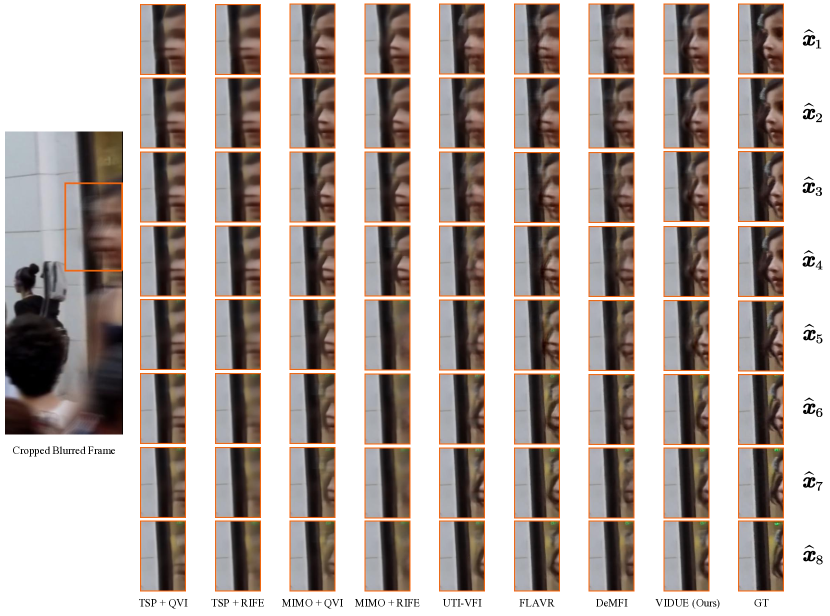
Figure S2: More visual results on GoPro [32] ($\times 8$).

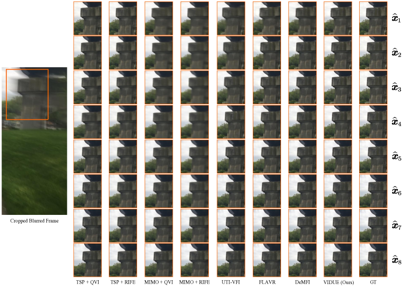
Figure S4: More visual results on Adobe [43] ($\times 8$).

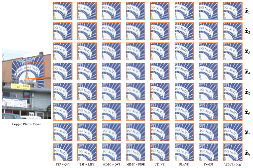
Figure S6: More visual results on RealBlur [43] ($\times 8$).

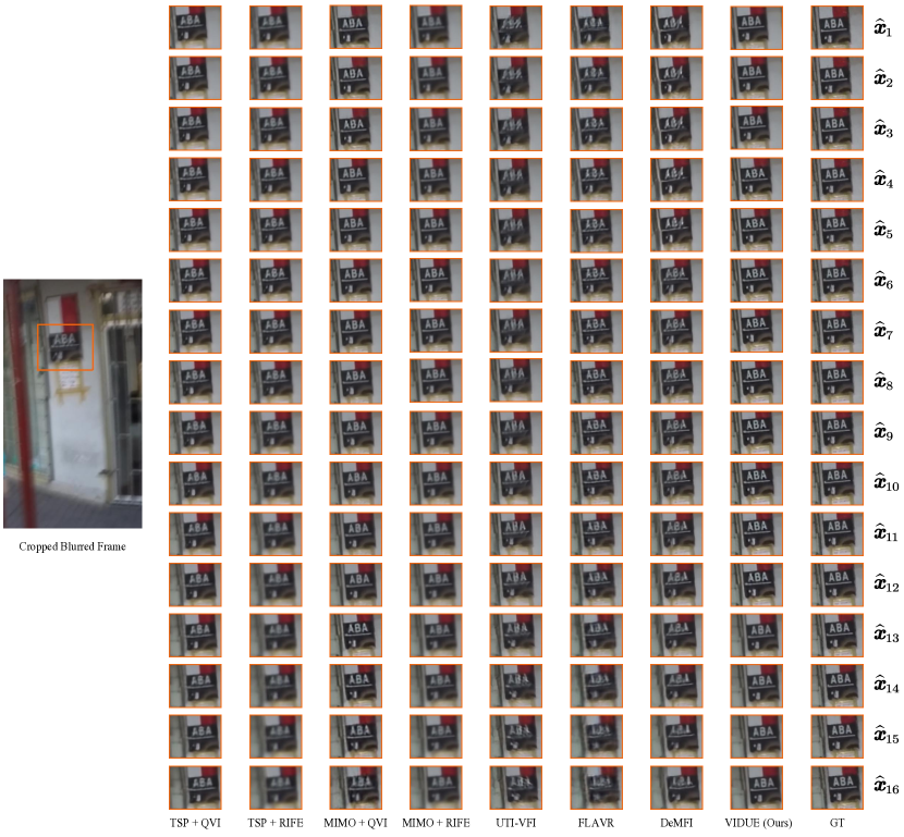
Figure S8: More visual results on GoPro [32] ($\times 16$).

References

- [1] Dawit Mureja Argaw, Junsik Kim, Francois Rameau, and In So Kweon. Motion-blurred video interpolation and extrapolation. In AAAI, pages 901–910, 2021.
- [2] Wenbo Bao, Wei-Sheng Lai, Chao Ma, Xiaoyun Zhang, Zhiyong Gao, and Ming-Hsuan Yang. Depth-aware video frame interpolation. In CVPR, pages 3703–3712, 2019.
- [3] Alan C Bovik. Handbook of Image and Video Processing. Academic Press, 2010.
- [4] Christian Brandli, Raphael Berner, Minhao Yang, Shih-Chii Liu, and Tobi Delbruck. A 240 180 130 dB 3 s latency global shutter spatiotemporal vision sensor. IEEE JSSC, 49:2333–2341, 2014.
- [5] Roberto Castagno, Petri Haavisto, and Giovanni Ramponi. A method for motion adaptive frame rate up-conversion. IEEE TCSVT, 6:436–446, 1996.
- [6] Tony F Chan and Chiu-Kwong Wong. Total variation blind deconvolution. IEEE TIP, 7:370–375, 1998.
- [7] Yen-Kuang Chen, Anthony Vetro, Huifang Sun, and Sun-Yuan Kung. Frame-rate up-conversion using transmitted true motion vectors. In MSPW, pages 622–627, 1998.
- [8] Zhixiang Chi, Rasoul Mohammadi Nasiri, Zheng Liu, Juwei Lu, Jin Tang, and Konstantinos N Plataniotis. All at once: Temporally adaptive multi-frame interpolation with advanced motion modeling. In ECCV, pages 107–123, 2020.
- [9] Sung-Jin Cho, Seo-Won Ji, Jun-Pyo Hong, Seung-Won Jung, and Sung-Jea Ko. Rethinking coarse-to-fine approach in single image deblurring. In ICCV, pages 4641–4650, 2021.
- [10] Byung-Tae Choi, Sung-Hee Lee, and Sung-Jea Ko. New frame rate up-conversion using bi-directional motion estimation. IEEE TCE, 46:603–609, 2000.
- [11] Myungsub Choi, Heewon Kim, Bohyung Han, Ning Xu, and Kyoung Mu Lee. Channel attention is all you need for video frame interpolation. In AAAI, pages 10663–10671, 2020.
- [12] Hongyun Gao, Xin Tao, Xiaoyong Shen, and Jiaya Jia. Dynamic scene deblurring with parameter selective sharing and nested skip connections. In CVPR, pages 3848–3856, 2019.
- [13] Pedro A Gutiérrez, Maria Perez-Ortiz, Javier Sanchez-Monedero, Francisco Fernandez-Navarro, and Cesar Hervas-Martinez. Ordinal regression methods: Survey and experimental study. IEEE TKDE, 28:127–146, 2015.
- [14] Tae H Kim, Kyoung M Lee, Bernhard Scholkopf, and Michael Hirsch. Online video deblurring via dynamic temporal blending network. In ICCV, pages 4038–4047, 2017.
- [15] Petri Haavisto, Janne Juhola, and Yrjö Neuvo. Fractional frame rate up-conversion using weighted median filters. IEEE TCE, 35:272–278, 1989.
- [16] Jie Hu, Li Shen, and Gang Sun. Squeeze-and-excitation networks. In CVPR, pages 7132–7141, 2018.
- [17] Zhewei Huang, Tianyuan Zhang, Wen Heng, Boxin Shi, and Shuchang Zhou. RIFE: Real-time intermediate flow estimation for video frame interpolation. In ECCV, pages 624–642, 2022.
- [18] Bo-Won Jeon, Gun-Ill Lee, Sung-Hee Lee, and Rae-Hong Park. Coarse-to-fine frame interpolation for frame rate up-conversion using pyramid structure. IEEE TCE, 49:499–508, 2003.
- [19] Huaizu Jiang, Deqing Sun, Varun Jampani, Ming-Hsuan Yang, Erik Learned-Miller, and Jan Kautz. Super SloMo: High quality estimation of multiple intermediate frames for video interpolation. In CVPR, pages 9000–9008, 2018.
- [20] Justin Johnson, Alexandre Alahi, and Li Fei-Fei. Perceptual losses for real-time style transfer and super-resolution. In ECCV, pages 694–711, 2016.
- [21] Tarun Kalluri, Deepak Pathak, Manmohan Chandraker, and Du Tran. FLAVR: Flow-agnostic video representations for fast frame interpolation. In WACV, pages 2071–2082, 2023.
- [22] Di Kang, Debarun Dhar, and Antoni Chan. Incorporating side information by adaptive convolution. In NeurIPS, pages 1–10, 2017.
- [23] Tero Karras, Samuli Laine, and Timo Aila. A style-based generator architecture for generative adversarial networks. In CVPR, pages 4401–4410, 2019.
- [24] Prannay Khosla, Piotr Teterwak, Chen Wang, Aaron Sarna, Yonglong Tian, Phillip Isola, Aaron Maschinot, Ce Liu, and Dilip Krishnan. Supervised contrastive learning. In NeurIPS, pages 18661–18673, 2020.
- [25] Taewoo Kim, Jeongmin Lee, Lin Wang, and Kuk-Jin Yoon. Event-guided deblurring of unknown exposure time videos. In ECCV, pages 1–34, 2022.
- [26] Tae H Kim, Mehdi SM Sajjadi, Michael Hirsch, and Bernhard Scholkopf. Spatio-temporal transformer network for video restoration. In ECCV, pages 106–122, 2018.
- [27] Diederik P Kingma and Jimmy Ba. Adam: A method for stochastic optimization. arXiv preprint arXiv:1412.6980, 2014.
- [28] Dilip Krishnan, Terence Tay, and Rob Fergus. Blind deconvolution using a normalized sparsity measure. In CVPR, pages 233–240, 2011.
- [29] Wei-Sheng Lai, Jian-Jiun Ding, Yen-Yu Lin, and Yung-Yu Chuang. Blur kernel estimation using normalized color-line prior. In CVPR, pages 64–72, 2015.
- [30] Hyeongmin Lee, Taeoh Kim, Tae-young Chung, Daehyun Pak, Yuseok Ban, and Sangyoun Lee. AdaCof: Adaptive collaboration of flows for video frame interpolation. In CVPR, pages 5316–5325, 2020.
- [31] Sreyas Mohan, Joshua L Vincent, Ramon Manzorro, Peter Crozier, Carlos Fernandez-Granda, and Eero P Simoncelli. Adaptive denoising via gaintuning. In NeurIPS, pages 23727–23740, 2021.
- [32] Seungjun Nah, Tae Hyun Kim, and Kyoung Mu Lee. Deep multi-scale convolutional neural network for dynamic scene deblurring. In CVPR, pages 3883–3891, 2017.
- [33] Simon Niklaus, Long Mai, and Feng Liu. Video frame interpolation via adaptive separable convolution. In ICCV, pages 261–270, 2017.
- [34] Jihyong Oh and Munchurl Kim. DeMFI: Deep joint deblurring and multi-frame interpolation with flow-guided attentive correlation and recursive boosting. In ECCV, pages 1–18, 2022.
- [35] Jinshan Pan, Haoran Bai, and Jinhui Tang. Cascaded deep video deblurring using temporal sharpness prior. In CVPR, pages 3043–3051, 2020.
- [36] Dongwon Park, Dong U Kang, Jisoo Kim, and Se Y Chun. Multi-temporal recurrent neural networks for progressive non-uniform single image deblurring with incremental temporal training. In ECCV, pages 327–343, 2020.
- [37] Ashish Raj and Ramin Zabih. A graph cut algorithm for generalized image deconvolution. In ICCV, pages 1048–1054, 2005.
- [38] Dongwei Ren, Kai Zhang, Qilong Wang, Qinghua Hu, and Wangmeng Zuo. Neural blind deconvolution using deep priors. In CVPR, pages 3341–3350, 2020.
- [39] Olaf Ronneberger, Philipp Fischer, and Thomas Brox. U-Net: Convolutional networks for biomedical image segmentation. In MICCAI, pages 234–241, 2015.
- [40] Wei Shang, Dongwei Ren, Dongqing Zou, Jimmy S Ren, Ping Luo, and Wangmeng Zuo. Bringing events into video deblurring with non-consecutively blurry frames. In ICCV, pages 4531–4540, 2021.
- [41] Wang Shen, Wenbo Bao, Guangtao Zhai, Li Chen, Xiongkuo Min, and Zhiyong Gao. Blurry video frame interpolation. In CVPR, pages 5114–5123, 2020.
- [42] Hyeonjun Sim, Jihyong Oh, and Munchurl Kim. XVFI: Extreme video frame interpolation. In ICCV, pages 14489–14498, 2021.
- [43] Shuochen Su, Mauricio Delbracio, Jue Wang, Guillermo Sapiro, Wolfgang Heidrich, and Oliver Wang. Deep video deblurring for hand-held cameras. In CVPR, pages 1279–1288, 2017.
- [44] Dmitry Ulyanov, Andrea Vedaldi, and Victor Lempitsky. Deep image prior. In CVPR, pages 9446–9454, 2018.
- [45] Xintao Wang, Kelvin CK Chan, Ke Yu, Chao Dong, and Chen C Loy. EDVR: Video restoration with enhanced deformable convolutional networks. In CVPRW, pages 0–0, 2019.
- [46] Zhou Wang, Alan C Bovik, Hamid R Sheikh, and Eero P Simoncelli. Image quality assessment: from error visibility to structural similarity. IEEE TIP, 13:600–612, 2004.
- [47] Gang Xu, Jun Xu, Zhen Li, Liang Wang, Xing Sun, and Ming-Ming Cheng. Temporal modulation network for controllable space-time video super-resolution. In CVPR, pages 6388–6397, 2021.
- [48] Xiangyu Xu, Siyao Li, Wenxiu Sun, Qian Yin, and Ming-Hsuan Yang. Quadratic video interpolation. In NeurIPS, pages 1–10, 2019.
- [49] Hongguang Zhang, Yuchao Dai, Hongdong Li, and Piotr Koniusz. Deep stacked hierarchical multi-patch network for image deblurring. In CVPR, pages 5978–5986, 2019.
- [50] Youjian Zhang, Chaoyue Wang, Stephen J Maybank, and Dacheng Tao. Exposure trajectory recovery from motion blur. IEEE TPAMI, 44:7490–7504, 2021.
- [51] Youjian Zhang, Chaoyue Wang, and Dacheng Tao. Video frame interpolation without temporal priors. In NeurIPS, pages 13308–13318, 2020.
- [52] Zhihang Zhong, Ye Gao, Yinqiang Zheng, and Bo Zheng. Efficient spatio-temporal recurrent neural network for video deblurring. In ECCV, pages 191–207, 2020.