Partially adaptive Multichannel joint reduction of ego-noise
and environmental noise

Abstract

Human-robot interaction relies on a noise-robust audio processing module capable of estimating target speech from audio recordings impacted by environmental noise, as well as self-induced noise, so-called ego-noise. While external ambient noise sources vary from environment to environment, ego-noise is mainly caused by the internal motors and joints of a robot. Ego-noise and environmental noise reduction are often decoupled, i.e., ego-noise reduction is performed without considering environmental noise. Recently, a variational autoencoder (VAE)-based speech model has been combined with a fully adaptive non-negative matrix factorization (NMF) noise model to recover clean speech under different environmental noise disturbances. However, its enhancement performance is limited in adverse acoustic scenarios involving, e.g. ego-noise. In this paper, we propose a multichannel partially adaptive scheme to jointly model ego-noise and environmental noise utilizing the VAE-NMF framework, where we take advantage of spatially and spectrally structured characteristics of ego-noise by pre-training the ego-noise model, while retaining the ability to adapt to unknown environmental noise. Experimental results show that our proposed approach outperforms the methods based on a completely fixed scheme and a fully adaptive scheme when ego-noise and environmental noise are present simultaneously.

Index Terms—  Ego-noise reduction, speech enhancement, variational autoencoder, multichannel non-negative matrix factorization

1 Introduction

In recent decades, research on autonomous systems (AS) such as humanoid interactive robots has received increasing attention. Interactive robots are typically equipped with multiple microphones to perceive their environment and react to requests or particular commands from humans. However, the acquisition of target acoustic information is often disturbed not only by external interfering sources, i.e., environmental noise, but also by self-generated noise, also called ego-noise. It poses difficulties for subsequent tasks, such as speech recognition and language understanding. This calls for a noise-robust audio processing module capable of recovering target clean speech to support the robot’s actuator unit to act appropriately [1, 2].

In human-robot interaction, ego-noise may originate from different parts of the robot and reducing ego-noise is non-trivial in various aspects. It is mainly caused by the electric motors and mechanical parts distributed all over the robot body [3, 4]. The microphones are often placed close to the motors, especially for small-sized robots, resulting in acoustic scenarios with challenging signal-to-noise ratios. Furthermore, as ego-noise coming from, e.g. robotic limb movements, is non-stationary, it may be considered a difficult noise source. However, due to the limited degree of motion, ego-noise from the motors and joints exhibits a characteristic spatial and spectral structure. Thus, specialized and efficient light-weight machine learning algorithms can be designed to learn and exploit these distinct spatial and spectral characteristics of ego-noise [1, 3, 4, 5, 6, 7, 8, 9, 10].

For instance, ego-noise can be modeled by dictionary-based algorithms, e.g.  non-negative matrix factorization (NMF) [11, 9, 12], where ego-noise is approximated by a linear combination of pre-captured dictionary components. For multichannel recordings, in addition to structured tempo-spectral characteristics, spatial information can also be employed using, e.g. multichannel NMF [6, 7]. Deleforge et al. [4] have proposed a sparse representation of multichannel ego-noise signals in the complex domain. Some approaches have included information from other modalities, such as motor data [5, 8, 12]. However, this requires synchronized multimodal data, which may not be readily available. While a pre-learned ego-noise model has shown some effectiveness in modeling noise characteristics, it may cause noise mismatch problems in realistic scenarios that include not only ego-noise, but also unknown environmental noise signals.

Currently, advanced methods for environmental noise reduction are based on deep neural networks (DNNs) [13]. The variational autoencoder (VAE) is a deep generative model that can be used to learn a probabilistic prior distribution of clean speech [14]. It has been combined with a statistical NMF noise model to perform speech enhancement, where the VAE-based speech model is pre-trained on clean speech while the parameters of the NMF model are estimated based on noisy observations [15, 16, 17]. The VAE-NMF framework has shown improved speech enhancement performance and generalization capabilities over its NMF counterpart and fully supervised baselines [15, 16, 17]. While the fully adaptive NMF noise model can potentially adapt to various acoustic scenarios, gaining robustness under adverse acoustic conditions (e.g. when ego-noise and environmental noise are present simultaneously) remains a challenging task, as we will show in experiments. Few existing publications take both ego-noise and environmental noise into account [10, 18, 19]. Ince et al. proposed to reduce stationary background noise independently of ego-noise [10]. Our previous work [18] has presented a single-channel joint noise reduction system for interactive robots, but disregarded spatial information.

In this work, we propose a multichannel joint ego-noise and environmental noise reduction method for interactive robots. For this, the tempo-spectral features of speech are modeled using the VAE and the noise characteristics are modeled by multichannel NMF as in [17]. More specifically, similar to multichannel ego-noise approaches such as [7], we want to take advantage of spatially and spectrally structured characteristics of ego-noise to gain robustness in adverse conditions. At the same time, similar to, e.g. [17], we want to retain the adaptation ability to unknown environmental noise. For this, we propose to model ego-noise and environmental noise separately. We pre-train the ego-noise model to capture the spectral and spatial features, while its temporal activation is adapted to noisy observations jointly with the parameters of the environmental noise model. Experimental results show the considerable benefits of the proposed joint reduction method when ego-noise and environmental noise are present simultaneously.

2 Signal Model

We consider an acoustic scenario where the target speech signal is disturbed by additive noise and recorded by a microphone array with $M$ channels. We transform the noisy mixture into the time-frequency domain using the  short-time Fourier transform (STFT):

$$\mathbf{X}_{ft}=\sqrt{g_{t}}\mathbf{S}_{ft}+\mathbf{N}_{ft}\,,$$ (1)

where $\mathbf{X}_{ft}\in\mathbb{C}^{M}$, $\mathbf{S}_{ft}\in\mathbb{C}^{M}$, and $\mathbf{N}_{ft}\in\mathbb{C}^{M}$ represent the complex coefficients of the mixture signal, the speech signal, and the noise signal at the frequency bin $f\in\{1,\cdots,F\}$ and the time frame $t\in\{1,\cdots,T\}$. $g_{t}$ is a gain parameter to increase the robustness to the time-varying loudness of speech sounds [17]. Note that the noise signals $\mathbf{N}_{ft}$ may contain either ego-noise or environmental noise or both. We aim to recover clean speech with improved quality and intelligibility given only noisy mixtures.

2.1 Noise model

The noise coefficients are assumed to follow a complex Gaussian distribution with zero mean

$$\vspace{-0.1cm}\mathbf{N}_{ft}\sim\mathcal{N}_{\mathbb{C}}(\boldsymbol{0},\ \mathbf{\Sigma}_{N,ft})\,,\vspace{-0.1cm}$$ (2)

where $\mathcal{N}_{\mathbb{C}}(\boldsymbol{\mu},\mathbf{\Sigma})$ denotes the complex Gaussian distribution with mean $\boldsymbol{\mu}$ and covariance matrix $\mathbf{\Sigma}$. The covariance matrix is defined as

$$\mathbf{\Sigma}_{N,ft}=\mathbf{R}_{N,f}\sigma_{N,ft}^{2},$$ (3)

where $\mathbf{R}_{N,f}\in\mathbb{C}^{M\times M}$ is a spatial covariance matrix characterizing the sound propagation process from sources to microphones. $\sigma_{N,ft}^{2}$ represents the noise spectral variance, which can be modeled using the NMF,

$$\vspace{-0.1cm}\sigma_{N,ft}^{2}=\left[\mathbf{W}_{N}\mathbf{H}_{N}\right]_{ft}=\sum_{k=1}^{K}w_{fk}h_{kt}\,,\vspace{-0.1cm}$$ (4)

where $\mathbf{W}_{N}\in\mathbb{R}^{F\times K}_{+}$ denotes the dictionary matrix that captures the time-frequency characteristics of noise and $\mathbf{H}_{N}\in\mathbb{R}^{K\times T}_{+}$ denotes the coefficient matrix that represents the temporal activity. The noise dictionary contains $K$ atoms indexed by $k$ ($K$ is also referred to here as the dictionary size). We will decompose the noise signal $\mathbf{N}_{ft}=\mathbf{E}_{ft}+\mathbf{B}_{ft}$ into ego-noise $\mathbf{E}_{ft}$ and environmental noise $\mathbf{B}_{ft}$ in Section 3.

2.2 Speech model

We assume that the clean speech coefficients are complex Gaussian-distributed:

$$\mathbf{S}_{ft}\sim\mathcal{N}_{\mathbb{C}}(\boldsymbol{0},\ \mathbf{\Sigma}_{S,f}\left(\mathbf{z}_{t})\right)\,,$$ (5)

where $\mathbf{\Sigma}_{S,f}(\mathbf{z}_{t})=\mathbf{R}_{S,f}\sigma_{S,f}^{2}(\mathbf{z}_{t})$. $\mathbf{R}_{S,f}\in\mathbb{C}^{M\times M}$ is the speech spatial covariance matrix. It is assumed that the speech tempo-spectral power can be inferred from the latent variable $\mathbf{z}_{t}\in\mathbb{R}^{L}$, denoted as $\sigma_{S,f}^{2}(\mathbf{z}_{t})$, which can be realized by the generative model of the VAE, i.e., the decoder. Let $\mathbf{s}_{t}\in\mathbb{C}^{F}$ be a vector of single-channel clean speech spectra at the $t$-th time frame. The posterior of the latent variable $q(\mathbf{z}_{t}|\mathbf{s}_{t})$ is approximated by a real-valued Gaussian distribution

$$\mathbf{z}_{t}|\mathbf{s}_{t}\sim\mathcal{N}(\mu_{z}(|\mathbf{s}_{t}|^{2}),\ \sigma_{z}(|\mathbf{s}_{t}|^{2}))\,,$$ (6)

where $\mu_{z}(|\mathbf{s}_{t}|^{2}):\mathbb{R}_{+}^{F}\rightarrow\mathbb{R}^{L}$ and $\sigma_{z}(|\mathbf{s}_{t}|^{2}):\mathbb{R}_{+}^{F}\rightarrow\mathbb{R}^{L}_{+}$ denote the nonlinear mapping from the power spectrogram to the mean and variance of the latent variable, implemented by the encoder of the VAE, also called the recognition model. The parameters of the VAE can be jointly learned by maximizing the variational lower bound of the log-likelihood $\log p(\mathbf{s}_{t})$

$$\mathcal{L}_{\text{VAE}}=\mathbb{E}_{q(\mathbf{z}_{t}|\mathbf{s}_{t})}\left[\log p(\mathbf{s}_{t}|\mathbf{z}_{t})\right]-\mathbb{KL}(q(\mathbf{z}_{t}|\mathbf{s}_{t})||p(\mathbf{z}_{t}))\,,$$ (7)

where $\mathbb{KL}(\cdot|\cdot)$ denotes the Kullback-Leibler divergence and $p(\mathbf{z}_{t})$ represents the standard Gaussian prior of $\mathbf{z}_{t}$.

2.3 Clean speech estimation

With the assumption that the speech and noise signals are independent, the noisy mixture is given by

$$\mathbf{X}_{ft}\sim\mathcal{N}_{\mathbb{C}}(\mathbf{0},\ g_{t}\mathbf{\Sigma}_{S,f}(\mathbf{z}_{t})+\mathbf{\Sigma}_{N,ft}).$$ (8)

The parameters of the VAE-based speech model are obtained by training the neural network on clean speech data. At testing, a Monte Carlo expectation maximization (MCEM) method can be employed to estimate the unknown parameters  {$\mathbf{W}_{N},\mathbf{H}_{N},\mathbf{R}_{N,f},\mathbf{R}_{S,f},g_{t}$} [17]. Finally, the multichannel Wiener filter is employed to extract clean speech

$$\vspace{-0.1cm}\widehat{\mathbf{S}}_{ft}=g_{t}\mathbf{\Sigma}_{S,f}(\mathbf{z}_{t})\left(g_{t}\mathbf{\Sigma}_{S,f}(\mathbf{z}_{t})+\mathbf{\Sigma}_{N,ft}\right)^{-1}\mathbf{X}_{ft}.$$ (9)

The fully adaptive scheme in [17] that optimizes the unknown parameters based on noisy inputs, will adapt flexibly to different types of noise without the need of prior information on potential noise structures. The main idea of this approach is to achieve a high generalization ability and robustness to unexpected noise types. However, if accurate prior knowledge is available, it can be very helpful to improve robustness, especially in acoustically challenging environments. Therefore, as ego-noise exhibits a very distinct spatial-spectral structure, prior knowledge can be efficiently exploited by pre-learning the dictionary matrix and the spatial covariance matrix on ego-noise recordings only. However, when only pre-learned on ego-noise, the flexibility and generalization to unseen scenarios is lost. For instance, rather poor performance is to be expected in environmental noise, which limits its applicability in realistic scenarios that contain both environmental noise and background noise.

3 Joint reduction of ego-noise
and environmental noise

In this section, we present a multichannel partially adaptive scheme, where we improve noise modeling capabilities by decomposing noise into ego-noise and environmental noise. This allows us to obtain a robust prior pre-learned on the distinct spatial and spectral characteristics of ego-noise, while retaining the flexibility to adapt to environmental noise signals.

3.1 Mixture model and speech estimation

In a real-world human-robot interaction scenario, a target speech signal may be distorted by ego-noise and environmental noise simultaneously. We, thus, consider a noise model that is comprised of ego-noise $\mathbf{E}_{ft}$ and environmental noise $\mathbf{B}_{ft}$ as follows:

$$\mathbf{N}_{ft}=\mathbf{E}_{ft}+\mathbf{B}_{ft}\,.$$ (10)

By assuming that the ego-noise, environmental noise and speech signals are independent and complex Gaussian distributed, the noisy mixture follows a complex Gaussian of the form:

$$\mathbf{X}_{ft}\sim\mathcal{N}_{\mathbb{C}}(\mathbf{0},\ g_{t}\mathbf{\Sigma}_{S,f}(\mathbf{z}_{t})+\mathbf{\Sigma}_{E,ft}+\mathbf{\Sigma}_{B,ft})\,,$$ (11)

where the covariance matrix of environmental noise is defined as $\mathbf{\Sigma}_{B,ft}=\mathbf{R}_{B,f}\left[\mathbf{W}_{B}\mathbf{H}_{B}\right]_{ft}$ with $\left[\mathbf{W}_{B}\mathbf{H}_{B}\right]_{ft}=\sum_{k_{b}=1}^{K_{B}}w_{fk_{b}}h_{k_{b}t}$, and the covariance matrix of ego-noise as $\mathbf{\Sigma}_{E,ft}=\mathbf{R}_{E,f}\left[\mathbf{W}_{E}\mathbf{H}_{E}\right]_{ft}$ with $\left[\mathbf{W}_{E}\mathbf{H}_{E}\right]_{ft}=\sum_{k_{e}=1}^{K_{E}}w_{fk_{e}}h_{k_{e}t}$. $K_{B}$ and $K_{E}$ are the sizes of the environmental noise dictionary and the ego-noise dictionary, respectively.

Similarly, clean speech can be estimated by applying the multichannel Wiener filter

$$\widehat{\mathbf{S}}_{ft}=g_{t}\mathbf{\Sigma}_{S,f}(\mathbf{z}_{t})(\mathbf{\Sigma}_{X,ft}(\mathbf{z}_{t}))^{-1}\mathbf{X}_{ft},$$ (12)

where $\mathbf{\Sigma}_{X,ft}(\mathbf{z}_{t})=g_{t}\mathbf{\Sigma}_{S,f}(\mathbf{z}_{t})+\mathbf{\Sigma}_{E,ft}+\mathbf{\Sigma}_{B,ft}$. This requires estimating the unknown parameters $\{\mathbf{W}_{E},\mathbf{H}_{E},\mathbf{W}_{B},\mathbf{H}_{B},\mathbf{R}_{S,f},\mathbf{R}_{E,f},\mathbf{R}_{B,f},\\ g_{t}\}$. The following subsections describe the estimation of the ego-noise dictionary matrix $\mathbf{W}_{E}$ and the spatial covariance matrix $\mathbf{R}_{E,f}$ using the pre-training technique, and an MCEM optimization method to the proposed partially adaptive scheme.

3.2 Training phase

To capture the spectral and spatial characteristics of ego-noise, we train a multichannel NMF model on ego-noise recordings by optimizing the negative log-likelihood:

$$\mathcal{L}=\sum_{f=1,t=1}^{F,T}\text{tr}\left(\mathbf{E}_{ft}\mathbf{E}_{ft}^{H}\mathbf{\Sigma}_{E,ft}^{-1}\right)+\ln\;\text{det}\left(\mathbf{\Sigma}_{E,ft}\right),$$ (13)

where constant terms are omitted [20]. $\text{tr}(\cdot)$ denotes the trace operator; $\text{det}(\cdot)$ denotes the determinant of a matrix; $\cdot^{H}$ denotes the conjugate transpose. Minimizing this function using the majorization scheme leads to the multiplicative update rules for $\{\mathbf{W}_{E},\mathbf{H}_{E},\mathbf{R}_{E,f}\}$ [17, 20]. We fix the dictionary matrix $\mathbf{W}_{E}$ and the spatial covariance matrix $\mathbf{R}_{E,f}$ at the testing phase, while keeping $\mathbf{H}_{E}$ adaptive to noisy observations to account for different temporal variations.

3.3 Parameter optimization

To estimate the unknown parameters in the testing phase, we follow the MCEM optimization scheme by [17]. At the Expectation step, the complete-data log-likelihood is approximated by averaging over $R$ samples:

$$\begin{split}\mathbf{Q}(\theta;\theta^{\ast})&=\mathbb{E}_{p(\mathbf{z}|\mathbf{X};\theta)}\left[\ln p(\mathbf{X},\mathbf{z};\theta)\right]\\ &\approx-\frac{1}{R}\sum_{r=1}^{R}\sum_{f=1,t=1}^{F,T}\biggl{[}\text{tr}\left(\mathbf{X}_{ft}\mathbf{X}_{ft}^{H}\left[\mathbf{\Sigma}_{X,ft}\left(\mathbf{z}_{t}^{(r)}\right)\right]^{-1}\right)\\ &+\ln\;\text{det}\left(\mathbf{\Sigma}_{X,ft}\left(\mathbf{z}_{t}^{(r)}\right)\right)\biggr{]}\,.\end{split}$$ (14)

$R$ samples of the latent variable are drawn using the Metropolis-Hastings algorithm with a Gaussian as a symmetric proposal distribution. $\theta^{\ast}$ is an initialization of the parameters. At the Maximization step, we minimize the loss function, i.e., the negative log-likelihood $-R\mathbf{Q}(\theta;\theta^{\ast})$, with respect to the unknown parameters $\theta=\{\mathbf{H}_{E},\mathbf{W}_{B},\mathbf{H}_{B},\mathbf{R}_{S,f},\mathbf{R}_{B,f},g_{t}\}$ using the auxiliary function technique. For this, equation (14) can be viewed as the superposition of a convex function (the first term) and a concave function (the second term), where the former can be bounded using the Jensen’s trace inequality and the latter can be bounded using a first-order Taylor expansion [17, Appendix A]. This gives an upper bound function and computing the partial derivative with respect to each parameter separately leads to the iterative update rules:

$$g_{t}=g_{t}^{*}\left[\frac{\displaystyle\sum_{r=1}^{R}\sum^{F}_{f=1}\sigma^{2}_{f}\left(\mathbf{z}_{t}^{(r)}\right)\text{tr}\left[\mathbf{M}_{ft}^{(r)}\mathbf{R}_{S,f}\right]}{\displaystyle\sum^{R}_{r=1}\sum^{F}_{f=1}\sigma^{2}_{f}\left(\mathbf{z}_{t}^{(r)}\right)\text{tr}\left[\left(\mathbf{\Sigma}_{X,ft}\left(\mathbf{z}_{t}^{(r)}\right)\right)^{-1}\mathbf{R}_{S,f}\right]}\right]^{\frac{1}{2}},$$ (15)

$$w_{fk_{b}}=w_{fk_{b}}^{*}\left[\frac{\displaystyle\sum_{r=1}^{R}\sum^{T}_{t=1}h_{k_{b}t}\text{tr}\left[\mathbf{M}_{ft}^{(r)}\mathbf{R}_{B,f}\right]}{\displaystyle\sum^{R}_{r=1}\sum^{T}_{t=1}h_{k_{b}t}\text{tr}\left[\left(\mathbf{\Sigma}_{X,ft}\left(\mathbf{z}_{t}^{(r)}\right)\right)^{-1}\mathbf{R}_{B,f}\right]}\right]^{\frac{1}{2}},$$ (16)

$$h_{k_{b}t}=h_{k_{b}t}^{*}\left[\frac{\displaystyle\sum_{r=1}^{R}\sum^{F}_{f=1}w_{fk_{b}}\text{tr}\left[\mathbf{M}_{ft}^{(r)}\mathbf{R}_{B,f}\right]}{\displaystyle\sum^{R}_{r=1}\sum^{F}_{f=1}w_{fk_{b}}\text{tr}\left[\left(\mathbf{\Sigma}_{X,ft}\left(\mathbf{z}_{t}^{(r)}\right)\right)^{-1}\mathbf{R}_{B,f}\right]}\right]^{\frac{1}{2}},$$ (17)

$$h_{k_{e}t}=h_{k_{e}t}^{*}\left[\frac{\displaystyle\sum_{r=1}^{R}\sum^{F}_{f=1}w_{fk_{e}}\text{tr}\left[\mathbf{M}_{ft}^{(r)}\mathbf{R}_{E,f}\right]}{\displaystyle\sum^{R}_{r=1}\sum^{F}_{f=1}w_{fk_{e}}\text{tr}\left[\left(\mathbf{\Sigma}_{X,ft}\left(\mathbf{z}_{t}^{(r)}\right)\right)^{-1}\mathbf{R}_{E,f}\right]}\right]^{\frac{1}{2}},$$ (18)

where $\mathbf{M}_{ft}^{(r)}=\left(\mathbf{\Sigma}_{X,ft}\left(\mathbf{z}_{t}^{(r)}\right)\right)^{-1}\mathbf{X}_{ft}\mathbf{X}_{ft}^{H}\left(\mathbf{\Sigma}_{X,ft}\left(\mathbf{z}_{t}^{(r)}\right)\right)^{-1}$.

The two adaptive spatial covariance matrices $\mathbf{R}_{S,f}$, $\mathbf{R}_{B,f}$ are updated by solving the corresponding algebraic Riccati equations as in the fully adaptive scheme [17] [20, Appendix I].

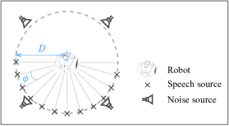
Fig. 1: Illustration of the recording setup with the NAO robot [21]. Room dimensions ($\text{length}\times\text{width}\times\text{height}$): $504\times 930\times 284$ cm; $T_{60}\approx 200~{}\text{ms}$; speaker-robot distance $D\approx 1~{}\text{m}$; $\phi\approx 15^{\circ}$.

4 Experiments

In this section, the proposed partially adaptive scheme (referred to as Partial) is compared to two baselines:

• Adaptive: Refers to the fully adaptive scheme with all unknown parameters estimated based on noisy observations [17].

• Fixed: Refers to the fixed scheme with the dictionary matrix and spatial covariance matrix pre-learned on ego-noise recordings at training time and fixed at test time as in the ego-noise reduction literature, e.g. [7, 6].

For each adaptive scheme, 7 different dictionary sizes are considered, leading to a total of 21 compared methods. We evaluate the algorithms in two application scenarios:

• Ego: Only ego-noise is present, mimicking a scene where a person is talking to a robot performing certain movements.

• Ego + Env: In addition to ego-noise, environmental noise is present simultaneously as an additional disturbance.

We use the scale-invariant signal-to-distortion ratio (Si-SDR) measured in dB to account for both noise reduction and the speech artifacts [22], and the perceptual objective listening quality analysis (POLQA) to measure speech quality [23]. The speech recognition accuracy is measured by the  word error rate (WER). We employ the pre-trained speech recognition model Quartznet [24] in the NeMo toolkit [25], in conjunction with a 4-gram language model available via the LibriSpeech website [26].

4.1 Dataset

All algorithms are trained and evaluated on a dataset recorded in our varechoic chamber. We use a humanoid interactive robot NAO H25 from Softbank for recording purposes [27]. The clean speech utterances are randomly chosen from the TIMIT test set [28]. Each target clean speech sample is played through a loudspeaker randomly placed among the positions shown in Fig. 1 and recorded using external omnidirectional electret microphones mounted in the same position of the built-in microphone array ($M=4$) on the robot. Ego-noise is recorded when the robot performs pre-defined right-arm movements in a crouching posture. To simulate external environmental noise sources, we re-record audio samples randomly selected from the DEMAND database [29] and the loudspeaker emitting environmental noise is placed at one of the four positions shown in Fig. 1. For the ego-noise only scenario, we mix speech signals with out-of-training ego-noise recordings (with movement speeds different from training data) at SNRs randomly chosen from {-5 dB, -4 dB, $\cdots$, 5 dB}. To simulate a challenging realistic scenario, besides ego-noise, we further corrupt speech signals by environmental noise at a SNR of 0 dB [17]. In total, this leads to a test set of 128 noisy samples for each evaluation scenario, with an average SNR of ${-2.1}$ dB for the joint noise scenario and ${-1.8}$ dB for the ego-noise only scenario.

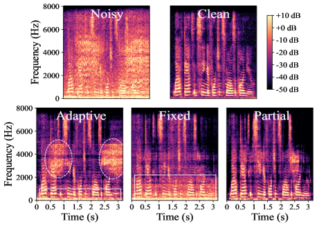
Fig. 2: Spectrograms of an audio example. Clean speech is distorted by both ego-noise and environmental noise. The three plots in the second row represent the reconstructed speech spectrograms obtained by three compared methods.

4.2 Hyperparameter settings

We use an STFT with a Hann window of 64 ms and a hop size of 25 %. All audio signals are sampled at 16 kHz. The decoder of the VAE has two hidden layers of sizes 128 and 512 respectively. The hyperbolic tangent activation function is applied to the hidden layers; the linear activation is applied to the output layer. The encoder network consists of two hidden layers of sizes 512 and 128, respectively, with the hyperbolic tangent activation functions applied. The latent dimension $L$ is set to 16. The VAE is trained on the re-recorded TIMIT training set using the same microphone setup as described in Section 4.1. The network parameters are optimized using the Adam optimizer with a learning rate of 0.001 and a patience of 5 epochs. The parameters of the MCEM algorithm are set as in [17], i.e., $R=10$ with a burn-in phase 30 iterations. For the partially adaptive scheme, we set the dictionary sizes for the fixed and adaptive parts as shown in Table 1.

Total dictionary size	16	32	64	96	128	160	192
$K_{B}$	8	16	32	32	32	32	32
$K_{E}$	8	16	32	64	96	128	160

Table 1: Dictionary sizes for the proposed partially adaptive scheme.

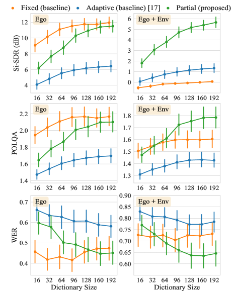
Fig. 3: Higher Si-SDR and POLQA scores indicate better enhancement performance, and lower WER indicates higher recognition accuracy. The marker denotes the mean value and the vertical bar indicates the 95%-confidence interval.

4.3 Results

The benefits of the partially adaptive scheme are visible in Fig. 2. While the fully adaptive scheme possesses the flexibility to adapt to various noisy conditions, its ability in capturing noise characteristics is limited especially when both ego-noise and environmental noise are present. This is shown by the residual ego-noise marked with the dashed ellipses and residual environmental noise marked with the solid rectangle in the reconstructed speech spectrogram. While the fixed scheme, whose reconstructed spectrogram is visualized in the second plot in the second row of Fig. 2, shows some effectiveness in removing ego-noise, the residual environmental noise is still quite pronounced, as marked by the solid rectangle. Finally, it can be observed that the proposed partially adaptive scheme shows a higher noise reduction effect than the other two approaches.

The two columns in Fig. 3 display the evaluation results for the ego-noise only scenario (Ego) and the joint noise scenario ($\text{Ego}+\text{Env}$), respectively. We observe that the fully adaptive approach is outperformed by the fully fixed and partially adaptive schemes in the presence of ego-noise only, as shown by its lowest POLQA and Si-SDR scores and the highest WER. This again implies that the fully adaptive scheme has difficulty in capturing ego-noise characteristics. The partially adaptive scheme and the fully adaptive scheme perform comparably when we increase the total dictionary size, indicating that ego-noise can be better modeled with a larger dictionary size due to its complexity and broadband characteristics. Eventually, it can be observed that the partially adaptive scheme delivers superior results over the other two methods when both noise types are present simultaneously. This indicates that with an appropriate dictionary size, the partially adaptive scheme can effectively approximate ego-noise while properly capturing unknown environmental noise in adverse scenarios. Audio examples are available online.

5 Conclusion

Based on the deep generative model and multichannel NMF, we proposed to jointly model ego-noise and environmental noise with a partially adaptive scheme. To exploit the spectrally and spatially structured characteristics of ego-noise, we pre-train the ego-noise model while keeping the environmental noise model adaptive to noisy observations. The proposed partially adaptive scheme demonstrated an increased performance compared to the approaches based on the fixed scheme and on the fully adaptive scheme in adverse scenarios where both ego-noise and environmental noise are present.

References

- [1] Alexander Schmidt, Heinrich W Löllmann, and Walter Kellermann, “Acoustic self-awareness of autonomous systems in a world of sounds,” Proceedings of the IEEE, vol. 108, no. 7, pp. 1127–1149, 2020.
- [2] Jorge Dávila-Chacón, Jindong Liu, and Stefan Wermter, “Enhanced robot speech recognition using biomimetic binaural sound source localization,” IEEE Trans. on Neural Networks and Learning Systems, vol. 30, no. 1, pp. 138–150, 2019.
- [3] Antoine Deleforge, Alexander Schmidt, and Walter Kellermann, “Audio-motor integration for robot audition,” in Multimodal Behavior Analysis in the Wild, pp. 27–51. Elsevier, 2019.
- [4] Antoine Deleforge and Walter Kellermann, “Phase-optimized K-SVD for signal extraction from underdetermined multichannel sparse mixtures,” in IEEE Int. Conf. Acoustics, Speech, Signal Proc. (ICASSP), Apr. 2015, pp. 355–359.
- [5] Alexander Schmidt, Heinrich W. Löllmann, and Walter Kellermann, “A novel ego-noise suppression algorithm for acoustic signal enhancement in autonomous systems,” in IEEE Int. Conf. Acoustics, Speech, Signal Proc. (ICASSP), Apr. 2018, pp. 6583–6587.
- [6] Alexander Schmidt and Walter Kellermann, “Multichannel nonnegative matrix factorization with motor data-regularized activations for robust ego-noise suppression,” in IEEE Int. Conf. on Autonomous Systems (ICAS), Aug. 2021, pp. 1–5.
- [7] Thomas Haubner, Alexander Schmidt, and Walter Kellermann, “Multichannel nonnegative matrix factorization for ego-noise suppression,” in Speech Communication; 13th ITG-Symposium, Oct. 2018, pp. 1–5.
- [8] Akinori Ito, Takashi Kanayama, Motoyuki Suzuki, and Shozo Makino, “Internal noise suppression for speech recognition by small robots,” in Ninth European Conf. on Speech Communication and Technology, 2005.
- [9] Taiki Tezuka, Takami Yoshida, and Kazuhiro Nakadai, “Ego-motion noise suppression for robots based on semi-blind infinite non-negative matrix factorization,” in IEEE Int. Conf. on Robotics and Automation (ICRA), May 2014, pp. 6293–6298.
- [10] Gökhan Ince, Kazuhiro Nakadai, Tobias Rodemann, Jun-ichi Imura, Keisuke Nakamura, and Hirofumi Nakajima, “Assessment of single-channel ego noise estimation methods,” in IEEE/RSJ Int. Conf. on Intelligent Robots and Systems, Sept. 2011, pp. 106–111.
- [11] Daniel Lee and H Sebastian Seung, “Algorithms for non-negative matrix factorization,” in Advances in Neural Information Proc. Systems, 2000, vol. 13.
- [12] Alexander Schmidt, Andreas Brendel, Thomas Haubner, and Walter Kellermann, “Motor data-regularized nonnegative matrix factorization for ego-noise suppression,” EURASIP Journal on Audio, Speech, and Music Processing, vol. 2020, no. 1, pp. 1–15, Dec. 2020.
- [13] DeLiang Wang and Jitong Chen, “Supervised speech separation based on deep learning: An overview,” IEEE/ACM Trans. Audio, Speech, Language Proc., vol. 26, no. 10, pp. 1702–1726, 2018.
- [14] Diederik P Kingma, Max Welling, et al., “An introduction to variational autoencoders,” Foundations and Trends® in Machine Learning, vol. 12, no. 4, pp. 307–392, 2019.
- [15] Simon Leglaive, Laurent Girin, and Radu Horaud, “A variance modeling framework based on variational autoencoders for speech enhancement,” in Int. Workshop on Machine Learning for Signal Processing (MLSP), Sept. 2018, pp. 1–6.
- [16] Kouhei Sekiguchi, Yoshiaki Bando, Kazuyoshi Yoshii, and Tatsuya Kawahara, “Bayesian multichannel speech enhancement with a deep speech prior,” in Asia-Pacific Signal and Information Proc. Association Annual Summit and Conf. (APSIPA ASC), Nov. 2018, pp. 1233–1239.
- [17] Simon Leglaive, Laurent Girin, and Radu Horaud, “Semi-supervised multichannel speech enhancement with variational autoencoders and non-negative matrix factorization,” in IEEE Int. Conf. Acoustics, Speech, Signal Proc. (ICASSP), May 2019, pp. 101–105.
- [18] Huajian Fang, Guillaume Carbajal, Stefan Wermter, and Timo Gerkmann, “Joint reduction of ego-noise and environmental noise with a partially-adaptive dictionary,” in Speech Communication; 14th ITG Conf., Sept. 2021, pp. 1–5.
- [19] Gökhan Ince, Ego Noise Estimation for Robot Audition, Ph.D. thesis, 2011.
- [20] Hiroshi Sawada, Hirokazu Kameoka, Shoko Araki, and Naonori Ueda, “Multichannel extensions of non-negative matrix factorization with complex-valued data,” IEEE Trans. Audio, Speech, Language Proc., vol. 21, no. 5, pp. 971–982, 2013.
- [21] Aldebaran Robotics, “NAOqi documentation center,” http://doc.aldebaran.com/.
- [22] Jonathan Le Roux, Scott Wisdom, Hakan Erdogan, and John R Hershey, “SDR–half-baked or well done?,” in IEEE Int. Conf. Acoustics, Speech, Signal Proc. (ICASSP), May 2019, pp. 626–630.
- [23] ITU-T Rec. P.863, “Perceptual objective listening quality prediction,” Int. Telecommunication Union, 2011.
- [24] Samuel Kriman, Stanislav Beliaev, Boris Ginsburg, Jocelyn Huang, Oleksii Kuchaiev, Vitaly Lavrukhin, Ryan Leary, Jason Li, and Yang Zhang, “Quartznet: Deep automatic speech recognition with 1d time-channel separable convolutions,” in IEEE Int. Conf. Acoustics, Speech, Signal Proc. (ICASSP), May 2020, pp. 6124–6128.
- [25] Oleksii Kuchaiev, Jason Li, Huyen Nguyen, Oleksii Hrinchuk, Ryan Leary, Boris Ginsburg, Samuel Kriman, Stanislav Beliaev, Vitaly Lavrukhin, Jack Cook, et al., “Nemo: a toolkit for building ai applications using neural modules,” arXiv preprint arXiv:1909.09577, 2019.
- [26] “openslr.org,” http://openslr.org/11/, 2022.
- [27] David Gouaillier, Vincent Hugel, Pierre Blazevic, Chris Kilner, Jérôme Monceaux, Pascal Lafourcade, Brice Marnier, Julien Serre, and Bruno Maisonnier, “Mechatronic design of NAO humanoid,” in IEEE Int. Conf. on Robotics and Automation (ICRA), May 2009, pp. 769–774.
- [28] John S., Garofolo and Lori F., Lamel and William M., Fisher and Jonathan G., Fiscus and David S., Pallett and Nancy L., Dahlgren and Victor Zue, “TIMIT acoustic-phonetic continuous speech corpus,” Linguistic data consortium, Philadelphia, 1993.
- [29] Joachim Thiemann, Nobutaka Ito, and Emmanuel Vincent, “The diverse environments multi-channel acoustic noise database (DEMAND): A database of multichannel environmental noise recordings,” in Proc. of Meetings on Acoustics ICA2013. Acoustical Society of America, June 2013, vol. 19, p. 035081.