Random measure priors in Bayesian frequency recovery from sketches

Abstract

Given a lossy-compressed representation, or sketch, of data with values in a set of symbols, the frequency recovery problem considers the estimation of the empirical frequency of a new data point. This is a classical problem in computer science, with recent studies applying Bayesian nonparametrics (BNPs) to develop learning-augmented versions of the popular count-min sketch (CMS) recovery algorithm. In this paper, we present a novel BNP approach to frequency recovery, which is not built from the CMS but still relies on a sketch obtained by random hashing. Assuming data to be modeled as random samples from an unknown discrete distribution, which is endowed with a Poisson-Kingman (PK) prior, we provide the posterior distribution of the empirical frequency of a symbol, given the sketch, from which estimates are obtained as mean functionals. An application of our result is presented for the Dirichlet process (DP) and Pitman-Yor process (PYP) priors, and in particular: i) we characterize the DP prior as the sole PK prior featuring a property of sufficiency with respect to the sketch, leading to a simple posterior distribution; ii) we identify a large sample regime under which the PYP prior leads to a simple approximation of the posterior distribution. We further develop our BNP approach to a general “traits” formulation of the frequency recovery problem, not yet studied in the CMS literature, in which data belong to more than one symbol, referred to as traits, and exhibit nonnegative integer levels of associations with each trait. In particular, by modeling data as random samples from a generalized Indian buffet process, we provide the posterior distribution of the empirical frequency level of a trait, given the sketch. This result is then applied under the assumption of a Poisson and Bernoulli distribution for the levels of associations, leading to a simple posterior distribution and a simple approximation of the posterior distribution, respectively.

Keywords: Bayesian nonparametrics; Dirichlet process; frequency recovery; generalized Indian buffet process; Pitman-Yor process; sketch; Poisson-Kingman prior; random hashing

1 Introduction

Recovering the empirical frequency of an object given a lossy-compressed representation, or sketch, of a large dataset is a classical problem in computer science [Misra and Gries, 1982; Alon et al., 1999; Manku and Motwani, 2002; Karp et al., 2003; Charikar et al., 2004; Cormode and Muthukrishnan, 2005; Indyk, 2006]. In its common “species" formulation, the frequency recovery problem considers $n\geq 1$ data points $(x_{1},\ldots,x_{n})$, with each $x_{i}$ taking one value in a (possibly infinite) set $\mathbb{S}$ of “species" labels or symbols, and it relies on a sketch of the $x_{i}$’s to recover the number of occurrences of a new $x_{n+1}$ in $(x_{1},\ldots,x_{n})$, namely the empirical frequency

$$f_{x_{n+1}}=\sum_{i=1}^{n}I(x_{i}=x_{n+1}),$$

with $I(\cdot)$ being the indicator function. The problem of recovering $f_{x_{n+1}}$ from a sketch of $(x_{1},\ldots,x_{n})$ is known to be relevant in diverse fields, including statistical machine learning in high-dimensional feature spaces [Shi et al., 2009; Aggarwal and Yu, 2010], cybersecurity in tracking password popularity [Schechter et al., 2010], web and social network data analysis [Song et al., 2009; Cormode, 2017], natural language processing [Goyal et al., 2012], sequencing analysis in biological sciences [Zhang et al., 2014; Berger et al., 2016; Solomon and Kingsford, 2016; Marcais et al., 2019; Leo Elworth et al., 2020], and privacy-protecting data analysis [Dwork et al., 2010; Melis et al., 2016; Cormode, 2017; Cormode et al., 2018; Kockan et al., 2020]. In general, sketching is practically motivated by memory limitations, as large numbers of distinct symbols in a dataset may otherwise be computationally expensive to analyze, or by privacy constraints, in situations where the data contain sensitive information. We refer to Cormode and Yi [2020, Chapter 3] for an up-to-date review on frequency recovery from sketches, and generalizations thereof.

The count-min sketch (CMS) [Cormode and Muthukrishnan, 2005] is arguably the most popular algorithm to recover $f_{x_{n+1}}$. It relies on a sketch obtained by $D\geq 1$ different $J$-wide independent random hash functions $h_{k}:\mathbb{S}\rightarrow\{1,\ldots,J\}$, for $k=1,\ldots,D$ and $J\geq 1$. Each function maps $(x_{1},\ldots,x_{n})$ into one of the $J$ buckets, defining a sketch $\mathbf{C}_{D,J}\in\mathbb{N}_{0}^{D\times J}$ whose $(k,j)$-th element $C_{k,j}$ counts the data points mapped by the $k$-th hash function into the $j$-th bucket. Then, based on $\mathbf{C}_{D,J}$, the CMS recovers $f_{x_{n+1}}$ by taking the smallest count among the $D$ buckets into which $x_{n+1}$ is mapped, i.e.

$$\hat{f}_{x_{n+1}}=\min\{C_{1,h_{1}(x_{n+1})},\ldots,C_{D,h_{D}(x_{n+1})}\}.$$ (1)

The CMS has been the subject of numerous studies, with a recent interest in the use of statistical models to better exploit the data [Cormode and Yi, 2020, Chapter 3]. In such a context, the work of Cai et al. [2018] is one of the most original contributions, introducing a Bayesian nonparametric (BNP) approach to obtain learning-augmented versions of the CMS. In particular, the $x_{i}$’s are assumed to be modeled as a random sample $(X_{1},\ldots,X_{n})$ from an unknown discrete distribution, which is endowed with a Dirichlet process (DP) prior [Ferguson, 1973], and then estimate $f_{X_{n+1}}$ are obtained as mean functionals of the posterior distribution of $f_{X_{n+1}}$ given $(C_{1,h_{1}(X_{n+1})},\ldots,C_{D,h_{D}(X_{n+1})})$, e.g. the mean, median and mode. Besides allowing to include some a priori knowledge on the data into the recovery problem, the BNP approach provides a natural way to assess uncertainty of estimates through the posterior distribution. See Dolera et al. [2021, 2023] for an extension to the more general Pitman-Yor process (PYP) prior [Pitman and Yor, 1997], which led to a novel learning-augmented CMS for power-law data.

1.1 Our contributions

In this paper, we present a novel BNP approach to frequency recovery. While the approach of Cai et al. [2018] is built from the CMS, hence the interest in a posterior distribution with respect to the same information of $\mathbf{C}_{D,J}$ as in (1), our approach considers BNP estimation of $f_{X_{n+1}}$ from a sketch obtained by a single random hash function, say $\mathbf{C}_{J}=(C_{1},\ldots,C_{J})\in\mathbb{N}_{0}^{J}$, computing the posterior distribution of $f_{X_{n+1}}$ with respect to $\mathbf{C}_{J}$. Within a (model-based) statistical perspective of the frequency recovery problem, our approach appears more natural than that of Cai et al. [2018], which may be questionable with respect to: i) the practical usefulness of combining a statistical model for the $x_{i}$’s with the sketch $\mathbf{C}_{D,J}$ from multiple hash functions, being such a sketch designed for a (model-free) recovery algorithm; ii) the use of a posterior distribution with respect to the sole $C_{k,h_{k}(X_{n+1})}$’s that may determine a loss of information, unless the $C_{k,h_{k}(X_{n+1})}$’s are somehow sufficient to estimate $f_{X_{n+1}}$. For the broad class of Poisson-Kingman priors [Pitman, 2003], which includes both the DP and PYP, we provide a closed-form expression for the posterior distribution of $f_{X_{n+1}}$ given $\mathbf{C}_{J}$ and the bucket in which $X_{n+1}$ is hashed, i.e. $h(X_{n+1})$. An application of our result to the DP prior shows that the posterior distribution depends on $\mathbf{C}_{J}$ only through $C_{h(X_{n+1})}$, thus proving that the BNP approach of Cai et al. [2018] relies on a sufficient statistic of $\mathbf{C}_{D,J}$; then, we characterize the DP prior as the sole PK prior that satisfies such a property of sufficiency. For the PYP, we show that the posterior distribution is intractable to be evaluated even for moderately large sample sizes, with a computational costs that scales exponentially in $J$; then, we identify a large sample regime that leads to a simple approximation of the posterior distribution, depending on $\mathbf{C}_{J}$ only through $C_{h(X_{n+1})}$. In general, our results show that, for priors beyond the DP, the BNP approach to frequency recovery leads to non-trivial computational challenges in the evaluation of the posterior distribution of $f_{X_{n+1}}$.

We further develop our BNP approach to a general “traits" formulation of the frequency recovery problem, not yet studied in the CMS literature, in which data belong to more than one symbol, referred to as traits, and exhibit nonnegative integer levels of associations with each trait [Campbell et al., 2018]. For examples, single cell data contain multiple genes with their expression levels, members of a social networks have friends to which they send multiple messages, documents contain different topics with their words. Here, we consider $n\geq 1$ data points $(x_{1},\ldots,x_{n})$, with each $x_{i}$ taking a value in a set $\mathbb{S}^{\infty}\times\mathbb{N}_{0}^{\infty}$ of traits with their levels, and assume the $x_{i}$’s to be modeled as a random sample $(X_{1},\ldots,X_{n})$ from the generalized Indian buffet process [James, 2017]. That is, the $X_{i}$’s are random counting measures, say $X_{i}=\sum_{k\geq 1}A_{i,k}\delta_{w_{k}}$, whose distribution is determined by: i) a distribution $G_{A}$ for the level of association $A_{i,k}\in\mathbb{N}_{0}$ of the trait $w_{k}\in\mathbb{S}$, which depends on a parameter $J_{k}>0$, for $k\geq 1$; ii) the distribution of a completely random measure (CRM) as a prior distribution for the $J_{k}$’s. Based on a sketch $\mathbf{C}_{J}\in\mathbb{N}_{0}^{J}$ of $(X_{1},\ldots,X_{n})$, still obtained by a single random hash function, we provide the posterior distribution of the empirical frequency level of a trait of a new $X_{n+1}$, given $\mathbf{C}_{J}$ and the bucket in which such a trait is hashed. It turns out that any CRM prior leads to a posterior distribution that depends on $\mathbf{C}_{J}$ only through $C_{h(X_{n+1})}$, showing a property of sufficiency as in the “species" formulation under the DP prior. We apply our result with $G_{A}$ being a Poisson distribution, which leads to a simple expression for the posterior distribution, and then we show how to use such an expression to approximate the posterior distribution with $G_{A}$ being a Bernoulli distribution. Our results show how the BNP approach to frequency recovery in the “species" formulation admits a natural extension to the “traits" formulation, for which we are not aware of any (model-free) algorithmic approach. This is a further evidence of the flexibility of the BNP approach to frequency recovery.

1.2 Organization of the paper

The paper is structured as follows. In Section 2 we consider the “species" formulation of frequency recovery: i) under PK priors, we compute the posterior distribution of the empirical frequency of a symbol; ii) we apply this result to the DP and the PYP priors, showing their peculiar properties within PK priors; iii) we present a numerical illustration. In Section 3 we consider the “traits" formulation of frequency recovery: i) under CRM priors, we compute the posterior distribution of the empirical frequency level of a trait; ii) we apply this result to the Poisson and the Bernoulli distribution for the level of association of traits; iii) we present a numerical illustration. Section 4 contains a discussion of our work, and some directions for future research. Proofs are deferred to Appendices.

2 BNP frequency recovery: “species" formulation

For $n\geq 1$, let $(x_{1},\ldots,x_{n})$ be data points with each $x_{i}$ taking a value in $\mathbb{S}$. The $x_{i}$’s are not observable, and instead we have access only to a sketch of them, which is obtained through random hashing [Mitzenmacher and Upfal, 2017, Chapter 5 and Chapter 15]. In particular, for an integer $J\geq 1$, let $h$ be a random hash function of width $J$, which is defined as a random mapping from $\mathbb{S}$ to $[J]=\{1,\ldots,J\}$ chosen from a pairwise independent hash family $\mathcal{H}_{J}$. That is, $h:\mathbb{S}\to[J]$, and, for any $j_{1},j_{2}\in[J]$ and fixed $x_{1},x_{2}\in\mathbb{S}$ such that $x_{1}\neq x_{2}$,

$$\text{Pr}[h(x_{1})=j_{1},\,h(x_{2})=j_{2}]=\frac{1}{J^{2}}.$$

The pairwise independence of $\mathcal{H}_{J}$, also known as strong universality, implies uniformity, meaning that $\Pr[h(x)=j]=J^{-1}$ for $j=1,\ldots,J$. The process of hashing $(x_{1},\ldots,x_{n})$ through $h$ produces a random vector $\mathbf{C}_{J}=(C_{1},\ldots,C_{J})\in\mathbb{N}_{0}^{J}$, which is referred to as sketch, whose $j$-th element (bucket) is

$$C_{j}=\sum_{i=1}^{n}I(h(x_{i})=j),$$

such that $\sum_{1\leq j\leq J}C_{j}=n$. In general, the sketch $\mathbf{C}_{J}$ has a smaller (physical) size than $(x_{1},\ldots,x_{n})$ due to the collisions of the $x_{i}$’s induced by random hashing [Cormode and Yi, 2020, Chapter 3]. The above sketch is a special version of the sketch $\mathbf{C}_{D,J}\in\mathbb{N}_{0}^{D\times J}$ at the basis of the CMS of Cormode and Muthukrishnan [2005], which simultaneously sketches the same data points $x_{i}$’s using a collection of $D\geq 1$ independent random hash functions from $\mathcal{H}_{J}$. We refer to Cormode and Yi [2020, Chapter 3] for further details on $\mathbf{C}_{D,J}$, and to Cai et al. [2018] for the use of $\mathbf{C}_{D,J}$ under a BNP model for the $x_{i}$’s.

Based of a sketch $\mathbf{C}_{J}$ of $(x_{1},\ldots,x_{n})$, we consider the problem of BNP estimation of the empirical frequency $f_{x_{n+1}}$. Following ideas first developed in Cai et al. [2018] and Dolera et al. [2023], the BNP approach to frequency recovery relies on two modeling assumptions: i) the data points $(x_{1},\ldots,x_{n})$ are modeled as a random sample $\mathbf{X}_{n}=(X_{1},\ldots,X_{n})$ from an unknown discrete distribution $P$, which is endowed by a nonparametric prior $\mathscr{P}$; ii) the hash family $\mathcal{H}_{J}$ is independent of $P$. Accordingly, we write the following BNP model:

$$\begin{split}C_{j}&\,=\,\sum_{i=1}^{n}I(h(X_{i})=j)\qquad j=1,\ldots,J\\[5.69046pt] h&\,\sim\,\mathcal{H}_{J}\\[5.69046pt] X_{1},\ldots,X_{n}\,|\,P&\,\stackrel{{\scriptstyle\mbox{\scriptsize{iid}}}}{{\sim}}\,P\\[5.69046pt] P&\,\sim\,\mathscr{P}.\end{split}$$ (2)

Under the model (2), the problem of recovering the empirical frequency $f_{X_{n+1}}$ from the sketch consists in the computation of the posterior distribution of $f_{X_{n+1}}$ given $\mathbf{C}_{J}$ and the buckets in which $X_{n+1}$ is hashed, i.e. $h(X_{n+1})$. Below, we compute such a posterior distribution assuming that $\mathscr{P}$ belongs to the broad class of PK priors, and then we apply our result to the DP prior and the PYP prior, which are arguably the most popular PK priors.

2.1 Main result

Before stating our main result, it is useful to recall the definition of PK prior [Pitman, 2003]. See also Pitman [2006, Chapter 3]. Consider a completely random measure (CRM) $\tilde{\mu}$ on $\mathbb{S}$, which is a random element with values on the space of bounded measure on $(\mathbb{S},\mathcal{S})$, such that for $k\geq 1$ and for a collection of disjoint Borel sets $A_{1},\ldots,A_{k}\in\mathcal{S}$ the random variables $\tilde{\mu}(A_{1}),\ldots,\tilde{\mu}(A_{k})$ are independent [Kingman, 1967]. We consider CRMs of the form

$$\tilde{\mu}(\cdot)=\int_{\mathbb{R}_{+}}s\tilde{N}(\mathrm{d}s,\,\cdot)=\sum_{k\geq 1}J_{k}\delta_{W_{k}}(\cdot),$$

where $\tilde{N}=\sum_{k\geq 1}\delta_{(J_{k},W_{k})}$ is a Poisson random measure on $\mathbb{R}_{+}\times\mathbb{S}$ with Lévy intensity $\nu(\mathrm{d}s,\mathrm{d}x)$, which characterizes the distribution of $\tilde{\mu}$ in terms its random jumps $J_{k}$’s and random locations $W_{k}$’s [Kingman, 1967, 1993]. We focus on homogeneous Lévy intensities, namely measures of the form $\nu(\mathrm{d}s,\,\mathrm{d}x)=\theta\rho(s)\mathrm{d}s\,G_{0}(\mathrm{d}x)$ where $\theta>0$ is a parameter, $G_{0}$ is a nonatomic probability measure on $\mathbb{S}$ and $\rho(s)\mathrm{d}s$ is a measure on $\mathbb{R}_{+}$ such that $\int_{\mathbb{R}_{+}}\rho(s)\mathrm{d}s=+\infty$ and

$$\psi(u)=\int_{\mathbb{R}_{+}}(1-e^{-us})\rho(s)\mathrm{d}s<+\infty$$ (3)

for all $u>0$, which ensure that $0<\tilde{\mu}(\mathbb{S})<+\infty$ almost surely [Pitman, 2003; Regazzini et al., 2003]. We write $\tilde{\mu}\sim\mbox{CRM}(\theta,\rho,G_{0})$ to denote an homogeneous CRM on $\mathbb{S}$. A PK prior is defined as the law of a suitable “normalization" of an homogeneous CRM with respect to its total mass [Pitman, 2003].

Definition 2.1.

Let $\tilde{\mu}\sim\mbox{CRM}(\theta,\rho,G_{0})$ with $T=\tilde{\mu}(\mathbb{S})\sim f_{T}$ and let $\text{PK}(\theta,\rho\,|\,T=t)$ be the conditional distribution of “normalized" random jumps $(J_{k}/T)_{k\geq 1}$ given $T=t$. If $g(\tilde{\mu})\equiv g(T)$ such that $\mathds{E}[g(T)]=1$, then a PK prior with parameter $(\theta,\rho,gf_{T},G_{0})$ is the law of the (discrete) random probability measure

$$P(\cdot)=\frac{\tilde{\mu}(\cdot)}{T}=\sum_{k\geq 1}\frac{J_{k}}{T}\delta_{W_{k}}(\cdot),$$

on $\mathbb{S}$, where the random probabilities $(J_{k}/T)_{k\geq 1}$ are distributed as the PK distribution $\text{PK}(\theta,\rho,gf_{T})=\int_{\mathbb{R}_{+}}\text{PK}(\theta,\rho\,|\,T=t)g(t)f_{T}(t)\mathrm{d}t$ and the random location $(W_{k})_{k\geq 1}$, independent of $(J_{k}/T)_{k\geq 1}$, are independent and identically distributed as $G_{0}$.

Under the model (2) with $\mathscr{P}$ being a PK prior, i.e. $P\sim\text{PK}(\theta,\rho,gf_{T},G_{0})$, the next theorem provides an expression for the posterior distribution of $f_{X_{n+1}}$ given $\mathbf{C}_{J}$ and $h(X_{n+1})$. Because of the broadness of the class of PK priors, this is a general result that can be applied upon suitable specifications of the measure $\rho$ and the function $g$. For instance, PK priors includes the class of (homogeneous) normalized CRM priors, which is obtained by setting $g$ as the identity function [James, 2002; Prünster, 2002; Pitman, 2003; Regazzini et al., 2003]. In general, it is sufficient to consider $g(t)\propto t^{-\gamma}e^{-\beta t}$ to recover from Definition 2.1 the most popular priors in BNPs. Common choices of $\tilde{\mu}$ are the Gamma CRM and the $\alpha$-Stable CRM [Kingman, 1975], as they provide PK priors with a flexible tail behaviour, ranging from geometric tail to heavy power-law tails, respectively. Under the Gamma CRM, Definition 2.1 provides a generalization of the DP prior, which is obtained by setting $g$ as the identity function. Under the $\alpha$-Stable CRM, Definition 2.1 provides a generalization of the normalized $\alpha$-Stable prior [Kingman, 1975], which is obtained by setting $g$ as the identity function, and it also includes the PYP prior and the normalized Gamma process prior [James, 2002; Lijoi et al., 2005, 2007]. We refer to [Pitman, 2006, Chapter 3] and Lijoi and Prünster [2010] for other examples of PK priors, with applications in BNPs. Applications of the next theorem to the DP and the PYP priors will be considered below, showing their peculiar features within the class of PK priors.

Theorem 2.2.

Let $\mathbf{C}_{J}$ be an observable sketch of $\mathbf{X}_{n}$ under the model (2) with $P\sim\text{PK}(\theta,\rho,gf_{T},G_{0})$ and $g(t)\propto t^{-\gamma}e^{-\beta t}$, and let $X_{n+1}$ be an additional (unobservable) random sample. With $\psi$ being defined in (3), if $\phi^{(n)}(u)=(-1)^{n}\frac{\mathrm{d}^{n}}{\mathrm{d}u^{n}}e^{-\theta/J\psi(u)}$ and $\kappa(u,n)=\int_{\mathbb{R}_{+}}e^{-un}s^{n}\rho(s)\mathrm{d}s$, then for $l=0,1,\ldots,c_{j}$

$$\mathrm{Pr}[f_{X_{n+1}}=l\,|\,\mathbf{C}_{J}=\mathbf{c},h(X_{n+1})=j]\\ \quad=\frac{\theta}{J}\binom{c_{j}}{l}\frac{\int_{\mathbb{R}_{+}}u^{n+\gamma}\phi^{(c_{j}-l)}(u+\beta)\prod_{k\neq j}\phi^{(c_{k})}(u+\beta)\,\kappa(u+\beta,l+1)\mathrm{d}u}{\int_{\mathbb{R}_{+}}u^{n+\gamma}\phi^{(c_{j}+1)}(u+\beta)\prod_{k\neq j}\phi^{(c_{k})}(u+\beta)\mathrm{d}u}.$$ (4)

See Appendix A.1 for the proof of Theorem 2.2. Theorem 2.2 provides a BNP solution of the problem of recovery $f_{X_{n+1}}$, in the sense that an estimator of $f_{X_{n+1}}$, with respect to a suitable loss function, is obtained as a mean functional of the posterior distribution (2.2). Also credible intervals may be derived. The use of a squared loss function is arguably the most common choice, leading the posterior mean as a BNP estimator of $f_{X_{n+1}}$, i.e.

$$\hat{f}_{X_{n+1}}=\sum_{l=0}^{c_{j}}l\,\text{Pr}[f_{X_{n+1}}=l\,|\,\mathbf{C}_{J}=\mathbf{c},h(X_{n+1})=j].$$

Theorem 2.2 extends the main results of Cai et al. [2018] and Dolera et al. [2023] with respect to both the use of the sketch and the specification of the prior distribution. As for the sketch, Cai et al. [2018, Proposition 1] and Dolera et al. [2023, Theorem 1 and Theorem 2] provide a posterior distribution of $f_{X_{n+1}}$ with respect to the sole bucket $C_{h(X_{n+1})}$ in which $X_{n+1}$ is hashed, whereas Theorem 2.2 considers the whole sketch $\mathbf{C}_{J}$ and where $X_{n+1}$ is hashed, i.e. $h(X_{n+1})$. As for the prior, Cai et al. [2018] and Dolera et al. [2023] focussed on the DP prior and PYP prior, obtaining posterior distributions by means of peculiar conjugacy or quasi-conjugacy properties of the priors, whereas here we consider a general PK prior. As discussed in Dolera et al. [2023], since the DP and PYP priors are the sole quasi-conjugate PK priors, the use of conjugacy properties is a strong limitation in view of considering more general prior distributions. Our proof of Theorem 2.2 overcomes this limitation, by avoiding the use of any form of conjugacy for the prior.

2.2 Results under the DP prior

We consider Definition 2.1 with $\tilde{\mu}$ being a Gamma CRM, i.e. $\rho(s)=s^{-1}\exp\{-s\}$, and $g$ being be the identity function. For this choice of $(\rho,g)$, $P\sim\text{PK}(\theta,\rho,gf_{T},G_{0})$ is a DP with mass $\theta>0$ and base measure $G_{0}$ [Ferguson, 1973; Pitman, 2003]. For short, we write $P\sim\text{DP}(\theta,G_{0})$. Then, the posterior distribution of $f_{X_{n+1}}$ given $\mathbf{C}_{J}$ and $h(X_{n+1})$ is obtained by an application of Theorem 2.2. Denote by $(a)_{(n)}$ the rising factorial of $a$ of order $n$, i.e. $(a)_{(n)}=\prod_{0\leq i\leq n-1}(a+i)$ with the proviso $(a)_{(0)}:=1$ [Charalambides, 2005, Chapter 2]. Then, from (4), for $l=0,1,\ldots,c_{j}$

$$\text{Pr}[f_{X_{n+1}}=l\,|\,\mathbf{C}_{J}=\mathbf{c},h(X_{n+1})=j]=\frac{\theta}{J}\frac{(c_{j}-l+1)_{(l)}}{\left(\frac{\theta}{J}+c_{j}-l\right)_{(l+1)}}.$$ (5)

See Appendix B.1 for the proof of (5) from 2.2, and Appendix B.2 for an alternative proof based on finite-dimensional properties of the DP. It is easy to show that (5) is a Beta-Binomial distribution, namely a Binomial distribution in which the probability of success at each of the $c_{j}$ trials is a Beta random variable with parameter $(1,\theta/J)$, say $B_{1,\theta/J}$. That is, if $F_{X_{n+1}}$ is a random variable distributed as (5), then by de Finetti theorem $c_{j}^{-1}F_{X_{n+1}}$ converges (weakly) to a $B_{1,\theta/J}$ as $c_{j}\rightarrow+\infty$. The posterior distribution (5) depends on $\mathbf{C}_{J}$ only through $C_{h(X_{n+1})}$. That is, under the DP prior, $C_{h(X_{n+1})}$ is a sufficient statistic for estimating $f_{X_{n+1}}$ from $\mathbf{C}_{J}$, thus making (5) equivalent to the posterior distribution computed in Cai et al. [2018, Proposition 1]. The next theorem shows that such an equivalence is a peculiar feature of the DP prior, characterizing the DP prior as the unique PK prior for which the posterior distribution of $f_{X_{n+1}}$ with respect to $C_{h(X_{n+1})}$ is equivalent to the posterior distribution with respect to $\mathbf{C}_{J}$ and $h(X_{n+1})$.

Theorem 2.3.

Under the setting of Theorem 2.2, the DP prior is the sole PK prior for which the posterior distribution (4) depends on $\mathbf{C}_{J}$ only through $C_{h(X_{n+1})}$.

See Appendix A.2 for the proof of Theorem 2.3. To conclude with the DP prior, we observe that a concrete application of the posterior distribution (5) requires to estimate the unknown prior’s parameter $\theta>0$ from the sketch $\mathbf{C}_{J}$. Cai et al. [2018] proposed an empirical Bayes approach to estimate $\theta$, which relies on the following finite-dimensional projective property of $P\sim\text{DP}(\theta,G_{0})$: if $\{B_{1},\ldots,B_{k}\}$ is a measurable $k$-partition of $\mathcal{S}$, for $k\geq 1$, then $(P(B_{1}),\ldots,P(B_{k}))$ is distributed as a Dirichlet distribution with parameter $(\theta G_{0}(B_{1}),\ldots,\theta G_{0}(B_{k}))$ [Ferguson, 1973; Regazzini, 2001]. According to the finite-dimensional projective property, and the assumption that $\mathcal{H}_{J}$ is independent of $P$, $\mathbf{C}_{J}$ is distributed as a Dirichlet-Multinomial distribution, i.e.

$$\text{Pr}[\mathbf{C}_{J}=\mathbf{c}]=\frac{n!}{(\theta)_{(m)}}\prod_{j=1}^{J}\frac{(\frac{\theta}{J})_{(c_{j})}}{c_{j}!}.$$ (6)

The fact that the distribution of $\mathbf{C}_{J}$ has a simple closed-form allows for an easy implementation of Bayesian estimation of $\theta$. Cai et al. [2018] adopted an empirical Bayes approach, which consists in estimating $\theta$ with the value that maximizes, over $\theta$, the (marginal) likelihood (6). Such a value is then used as a plug-in estimate in the posterior distribution (5). Alternatively, a fully Bayes approach can be applied by placing a prior distribution on $\theta$ and evaluating the induced posterior distributions through Monte Carlo sampling.

2.3 Results under the PYP prior

We consider Definition 2.1 with $\theta=1$, $\tilde{\mu}$ being an $\alpha$-Stable CRM, i.e. $\rho(s)=(\alpha/\Gamma(1-\alpha))s^{-1-\alpha}$ for $\alpha\in(0,1)$ and $g(t)=(\Gamma(\gamma+1)/\Gamma(\gamma/\alpha+1)t^{-\gamma}$ for $\gamma>-\alpha$, with $\Gamma(\cdot)$ being the Gamma function, i.e. $\Gamma(x)=\int_{(0,+\infty)}z^{x-1}\text{e}^{-z}\mathrm{d}z$ for $x>0$. For this choice of $(\theta,\rho,g)$, $P\sim\text{PK}(\theta,\rho,gf_{T},G_{0})$ is a PYP with discount $\alpha$, mass $\gamma$ and base measure $G_{0}$ [Pitman, 2003]. For short, we write $P\sim\text{PYP}(\alpha,\gamma,G_{0})$. Then, the posterior distribution of $f_{X_{n+1}}$ given $\mathbf{C}_{J}$ and $h(X_{n+1})$ is obtained by an application of Theorem 2.2. Denote by $\mathscr{C}(n,k;s)$ the generalized factorial of $n$ of order $k$, i.e.

$$\mathscr{C}(n,k;s)=\frac{1}{k!}\sum_{i=0}^{k}(-1)^{i}{n\choose i}(-is)_{(n)}$$

[Charalambides, 2005, Chapter 2 and Chapter 3]. Then, from (4), for $l=0,1,\ldots,c_{J}$

$$\text{Pr}[f_{X_{n+1}}=l\,|\,\mathbf{C}_{J}=\mathbf{c},h(X_{n+1})=j]\\ \quad=\frac{\gamma}{J}\binom{c_{j}}{l}(1-\alpha)_{(l)}\frac{\sum_{\bm{i}\in\mathcal{S}(\bm{c},j,-l)}\frac{\Gamma\left(\frac{\gamma+\alpha}{\alpha}+|\bm{i}|\right)}{J^{|\bm{i}|}}\prod_{k=1}^{J}\mathscr{C}(c_{k}-l\delta_{k,j},i_{k};\alpha)}{\sum_{\bm{i}\in\mathcal{S}(\bm{c},j,1)}\frac{\Gamma\left(\frac{\gamma}{\alpha}+|\bm{i}|\right)}{J^{|\bm{i}|}}\prod_{k=1}^{J}\mathscr{C}(c_{k}+\delta_{k,j},i_{k};\alpha)},$$ (7)

where $\mathcal{S}(\bm{c},j,q)$ is the Cartesian product of the index sets $\{\{0,\ldots,c_{k}+\delta_{k,j}q\},\ k=1,\ldots,J\}$, and for a multi-index $\bm{i}\in\mathcal{S}(\bm{c},j,q)$, $|\bm{i}|=\sum_{k=1}^{J}i_{k}$. See Appendix C.1 for the proof of (7). Note that the posterior distribution (7) depends on the whole sketch $\mathbf{C}_{J}$, with the size of $\mathcal{S}(\bm{c},j,q)$ blowing up exponentially both in $J$ and in $n$, e.g. if $J=10$ and $c_{j}=5$ for all $j$, then $|\mathcal{S}(\bm{c},j,q)|\approx 60\times 10^{6}$. This makes (7) intractable to be evaluated even for moderately large sample sizes, as it involves summations over a potentially very large number of generalized factorial coefficients, depending on $J$. We refer to Appendix C.2 for some approaches to evaluate (7), leading to some non-trivial computational challenges. The next theorem provides a large sample (qualitative) approximation of (7), which depends on $\mathbf{C}_{J}$ only through $C_{h(X_{n+1})}$.

Theorem 2.4.

The posterior distribution (7) is such that, if $n\rightarrow+\infty$ and $c_{k}\rightarrow+\infty$ simultaneously for any $k\neq j$ while $c_{j}$ is fixed, then for any fixed $l\geq 0$

$$\mathrm{Pr}[f_{X_{n+1}}=l\,|\,\mathbf{C}_{J}=\mathbf{c},h(X_{n+1})=j]$$ (8)

$$\quad\rightarrow\gamma{c_{j}\choose l}(1-\alpha)_{(l)}\frac{\Gamma\left(\frac{\gamma}{\alpha}+J\right)(\gamma+J\alpha)_{(c_{j}-l)}}{\Gamma\left(\frac{\gamma}{\alpha}+J-1\right)(\gamma+J\alpha-\alpha)_{(c_{j}+1)}}.$$

See Appendix A.3 for the proof of Theorem 2.3. As for the DP prior, a concrete application of the posterior distribution (7), as well as its large sample asymptotic approximation arising from (8), requires to estimate the unknown prior’s parameter $(\alpha,\gamma)$ from the sketch $\mathbf{C}_{J}$. As discussed in Dolera et al. [2023], under the PYP prior the distribution of $\mathbf{C}_{J}$ has not a simple closed-form expression, thus preventing the use of an empirical Bayes or fully Bayes approach to estimate $(\alpha,\gamma)$. Dolera et al. [2023] adopted a likelihood-free approach based on the Wasserstein distance [Bernton et al., 2019], whereby independent data sets $\mathbf{X}^{\prime}_{n}$ are sampled from $P\sim\text{PYP}(\alpha^{\prime},\gamma^{\prime},G_{0})$ and subsequently sketched into $\mathbf{C}^{\prime}_{J}$ with the same hash function $h$. The sketches $\mathbf{C}_{J}$ and $\mathbf{C}^{\prime}_{J}$ are then compared by means of the 1-Wasserstein distance and the empirical estimates for $(\alpha,\gamma)$ are defined as those minimizing (a suitable approximation of) the Wasserstein distance between $\mathbf{C}^{\prime}_{J}$ and $\mathbf{C}_{J}$. This approach is computationally demanding, as it requires to compute the Wasserstein distance, which has a computational cost of $\mathcal{O}(J^{3})$, and to simulate $\mathbf{X}^{\prime}_{n}$ whose cost scales super-linearly with $n$, depending on the parameters’ values. Since the objective function is not differentiable, Dolera et al. [2023] made use of Bayesian Optimization to find the estimates for the parameters. Here, instead, we propose to consider the first $n^{\prime}\ll n$ observations, sketch them through $h$ and estimate their frequency through the expected value of (8). Minimizing the mean absolute error of the frequency recovery with respect to the parameters is easy since the loss function is differentiable (almost everywhere) and can be done with standard software packages.

2.4 Numerical illustrations

We present an illustration for the posterior distributions under the DP prior and the PYP prior, i.e. Equation (5) and Equation (7), respectively. We set $n=50$ and $J=10$, and we consider four sketched datasets, say $\mathbf{C}_{J}^{\text{\tiny{(1)}}}$, $\mathbf{C}_{J}^{\text{\tiny{(2)}}}$, $\mathbf{C}_{J}^{\text{\tiny{(3)}}}$, and $\mathbf{C}_{J}^{\text{\tiny{(4)}}}$, whose values are reported in Table 1. In particular: i) for the scenario $\mathbf{C}_{J}^{\text{\tiny{(1)}}}$, the values $C^{\text{\tiny{(1)}}}_{j}$’s are constant across $j$; ii) for the scenario $\mathbf{C}_{J}^{\text{\tiny{(2)}}}$, the values $C^{\text{\tiny{(2)}}}_{j}$’s decay exponentially in $j$; iii) for the scenario $\mathbf{C}_{J}^{\text{\tiny{(3)}}}$, the values $C^{\text{\tiny{(3)}}}_{j}$’s decay linearly in $j$; iv) for scenario $\mathbf{C}_{J}^{\text{\tiny{(4)}}}$ the values $C^{\text{\tiny{(4)}}}_{j}$’s are either equal to nine, five, or one. Moreover, we assume that $X_{n+1}$ is mapped into the bucket $h^{(i)}(X_{n+1})$ such that $C^{\text{\tiny{(i)}}}_{h^{(i)}(X_{n+1})}=5$ for $i=1,2,3,4$. We consider a PYP prior with parameter $\gamma=1$ and parameter $\alpha=0,\,0.1,\,0.3,\,0.5$; recall that the PYP prior with parameter $\alpha=0$ and $\gamma>0$ coincides with the DP prior with parameter $\gamma$. Figure 1 summarizes the posterior distribution of $f_{X_{n+1}}$ for the three different scenarios. Given the sufficiency of $C_{h(X_{n+1})}$ under the DP prior, the corresponding posterior distributions do not change across the different scenarios; moreover, the posterior distributions under the DP prior are the most concentrated on larger values. We observe that, for all the different scenarios, increasing the parameter $\alpha$ corresponds to pushing the posterior to lower values. Finally, there are some differences in the posterior distributions under the PYP priors across the different scenarios, although these are not so evident from the plots. In particular, for $\alpha=0.3$ and $\alpha=0.5$, under setting $i=2$ the posterior mass assigned to 5 is slightly larger than in the other settings.

$\mathbf{C}_{J}^{\text{\tiny{(1)}}}$	5	5	5	5	5	5	5	5	5	5
$\mathbf{C}_{J}^{\text{\tiny{(2)}}}$	14	10	7	5	4	3	2	2	2	1
$\mathbf{C}_{J}^{\text{\tiny{(3)}}}$	10	9	8	7	5	4	3	2	1	1
$\mathbf{C}_{J}^{\text{\tiny{(4)}}}$	9	9	9	5	5	5	5	1	1	1

Table 1: Empirical frequencies of the $j$-th bucket (by column) in each simulated scenario (by row).

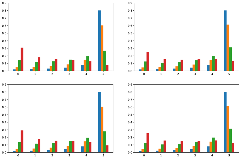
Figure 1: Posterior distribution of $f_{X_{n+1}}$ in the four different scenarios. In each plot, the blue, orange, green, and red bars correspond to $\alpha$ equal to $0$, $0.1$, $0.3$, and $0.5$ respectively, while $\gamma=1$.

As a further illustration of our results, we consider $n=500,000$ data points generated from a Dirichlet process with parameter $\theta=5,10,20,100$, and from a Zipf distribution with parameter $c=1.18,1.54,1.82,2.22$, which is typically used to model frequencies with power-law tail behavior. In particular, we recall that the parameter $c$ controls the tails of the Zipf distribution, with lower values of $c$ corresponding to heavier tails (i.e., larger fractions of types with a low frequency). We assume a DP prior, and estimate its total mass by maximizing (6) using the Python package JAX. We let $J$ vary between $100$ and $5,000$. We assess the goodness of (5) by comparing the a posteriori expected value with the true frequency of each token in the dataset, and compute the mean absolute error (MAE) stratified by the true frequency of the tokens. As shown in Figure 2, in the well specified settings the MAEs for low and mid frequency tokens decrease rapidly with $J$ especially when the parameter $\theta$ is small. On the other hand, for data generated from the Zipf distribution, the MAEs are considerably larger, especially when $c$ is small. Such a behaviour is not surprising, since the DP prior is known to be suitable for modeling discrete distributions with geometric tails, thus not being able to capture the power-law behavior of the Zipf distribution.

Finally, we consider the same synthetic datasets of Dolera et al. [2023], which consist of $n=500,000$ samples from the Zipf distribution with parameter $c=1.18,1.54,1.82,2.22$. We make use of (8) to estimate the frequencies via the posterior expectation, and then we compare estimating the parameters via the likelihood-free approach in Dolera et al. [2023] (specifically, we refer to their estimated values) and our method based on minimizing the recovery error on the first 10,000 samples. Results are displayed in Figure 3. Note that, in order to satisfy the asymptotic regime of Theorem 2.4, we fix $J$ to smaller values than the previous simulation. It is clear that the proposed method of estimation yields to a substantial improvement for the frequency recovery problem. Moreover, the use of a PYP prior results in much lower MAEs compared to a DP prior, especially for low frequency tokens. Interestingly, while under the DP prior larger values of the parameter $c$ correspond to better performance, under the PYP it is the opposite. This can be explained by the fact that when $c$ is large, there will be a small number of data points that contribute to most of the total mass, typically referred to as heavy hitters. Hence, when predicting the frequency of the heavy hitters, the asymptotic regime under which (8) is derived does not hold, as it can be the case that $c_{j}$ is comparable to $n$ for some $j$. Similarly, if $J$ is large, it might happen that $c_{j}\approx 0$ for some values of $j$, which also justifies the fact that for $c=1.82$ the performance of deteriorates as the Zipf’s exponent $c$ increases.

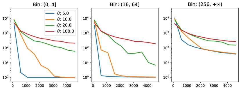
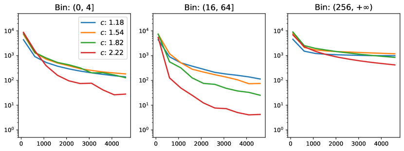
Figure 2: MAEs as a function of $J$ for the frequency recovery problem under the DP prior. Top row: data simulated from a Dirichlet process. Bottom row: data generated from the Zipf distribution.

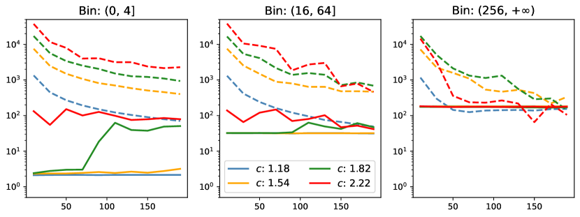
Figure 3: MAEs as a function of $J$ for the frequency recovery problem of Zipfian data under the PYP prior. Solid lines correspond to prior’s parameters $(\alpha,\theta)$ estimated using our method, whereas dashed lines correspond to prior’s parameters $(\alpha,\theta)$ estimated as in Dolera et al. [2023].

3 BNP frequency recovery: “traits" formulation

The “traits" formulation of the frequency recovery problem generalizes the “species" formulation by assuming that data belong to more than one symbol, referred to as traits, and exhibit nonnegative integer levels of associations with each trait. We assume $n\geq 1$ data points $(x_{1},\ldots,x_{n})$ to be modeled as a random sample $\mathbf{X}_{n}=(X_{1},\ldots,X_{n})$, whose BNP model will be specified below, with each $X_{i}$ taking a value in the set $\mathbb{S}^{\infty}\times\mathbb{N}_{0}^{\infty}$. That is, we write $X_{i}=((\tilde{Y}_{i,j},\tilde{A}_{i,j}),j=1,\ldots,K_{i})$, with the $\tilde{A}_{i,j}$’s being the levels of associations in $\mathbb{N}_{0}$ and the $\tilde{Y}_{i,j}$’s being the traits’ labels in $\mathbb{S}$. The sketch of $\mathbf{X}_{n}$ is performed at the trait level: a random hash function $h:\mathbb{S}\rightarrow\{1,\ldots,J\}$ from the hash family $\mathcal{H}_{J}$ is applied to the traits $\tilde{Y}_{i,j}$’s of $\mathbf{X}_{n}$, in such a way that each $\tilde{Y}_{i,j}$ is hashed in a bucket whose counter $C_{h(\tilde{Y}_{i,j})}$ is incremented by the corresponding level of association $\tilde{A}_{i,j}$, for $j=1,\ldots,K_{i}$ and $i=1,\ldots,n$. Such a process of hashing $\mathbf{X}_{n}$ through $h$ produces a sketch $\mathbf{C}_{J}=(C_{1},\ldots,C_{J})$ whose $j$-th bucket contains the sum of the levels of associations of the traits that are hashed in $j$, for $j=1\ldots,J$. Denoting by $Y_{n+1,\ell}$ a trait belonging to a new data point $X_{n+1}$, we define the empirical frequency level of $Y_{n+1,\ell}$ as

$$f_{Y_{n+1,\ell}}=\sum_{i=1}^{n}\sum_{j=1}^{K_{i}}\tilde{A}_{i,j}I(\tilde{Y}_{i,j}=Y_{n+1,\ell}).$$ (9)

Based on the sketch $\mathbf{C}_{J}$ of $\mathbf{X}_{n}$, we consider the problem of BNP estimation of $f_{Y_{n+1,\ell}}$, assuming that $\mathbf{X}_{n}$ is a random sample from the generalized Indian buffet process [James, 2017]. Under this modeling assumption, the frequency levels of “traits" are sufficient statistics for the $X_{i}$’s [Campbell et al., 2018], as were the frequencies of “species" within the BNP model for the $X_{i}$’s in Section 2.

Topic modeling is one of the most popular applications of “traits" allocations. In particular, consider the problem of classifying documents into topics using a multinomial naive Bayes classifier. Let $(X_{i},T_{i})$ be a data point, where $T_{i}\in\{1,\ldots,M\}$ is a topic label. Let $n_{j}$ be the number of the documents in each topic. Under the naive Bayes assumption, the classification rule is

$$\mathrm{Pr}[T_{i}=m\,|\,X_{i}=\{(y_{i,j},a_{i,j})\}_{j=1}^{K_{i}}]\propto\mathrm{Pr}[T_{i}=m]\prod_{j=1}^{K_{i}}(\pi^{m}_{y_{i,j}})^{a_{i,j}},$$ (10)

where $\pi^{m}_{y_{i,j}}$ is the relative frequency of $y_{i,j}$ in the subset of the documents for which $T_{i}=m$. Then, one may consider a sketched version of (10), in which $\pi^{m}_{y_{i,j}}$ is replaced by the Bayesian estimator $\hat{f}^{m}_{y_{i,j}}/n_{j}$ from sketched data. Another application is in feature engineering, by computing sketched “tf-idfs”. In information retrieval, tf-idf is a prominent pre-processing step, which consists in weighting the $\tilde{A}_{i,k}$’s by the (logarithm of the) inverse of the number of documents displaying the trait $\tilde{Y}_{i,k}$. That is, the level of association for $\tilde{Y}_{i,k}$ is

$$\frac{\tilde{A}_{i,k}}{\sum_{j=1}^{K_{i}}\tilde{A}_{i,j}}\log\frac{n}{\sum_{i=1}^{n}I(\tilde{Y}_{i,k}\in X_{i})}.$$ (11)

It is also common wisdom that such tf-idfs can be used in place of the raw frequencies in (10) [Rennie et al., 2003]. One may consider a sketched version of (11), in which the counter is incremented by one instead of $\tilde{A}_{i,k}$ so that $f_{Y_{n+1},\ell}$ is exactly the count of how many documents contain word $Y_{n+1}$. Finally, we mention the work by Zhou et al. [2016], which combines some ideas from the naive Bayes approach with a BNP model for “traits" allocations.

3.1 BNP model and main result

It is useful to start with the definition of the generalized Indian buffet process, which is arguably one of the most popular framework for BNP modeling of “traits" allocations. See also Broderick et al. [2015], Broderick et al. [2018], and references therein, for a detailed account of BNP modeling of “traits" allocations, and generalizations thereof.

Definition 3.1.

Let $\tilde{\mu}\sim\text{CRM}(\theta,\rho,G_{0})$, that is $\tilde{\mu}=\sum_{k\geq 1}J_{k}\delta_{W_{k}}$, and let $G_{A}$ be a probability mass function over $\mathbb{N}_{0}$. We say that a random variable $X$ given $\tilde{\mu}$ is distributed as a generalized Indian buffet process with parameter $G_{A}$ if

$$X=\sum_{k\geq 1}A_{k}\delta_{W_{k}},$$

where $(A_{k})_{k\geq 1}$ is independent of $(W_{k})_{k\geq 1}$ and such that $A_{k}\,|\,J_{k}\sim G_{A}(J_{k})$ for $k\geq 1$.

For short, we write $X\,|\,\tilde{\mu}\sim\mbox{IBP}(G_{A}\,|\,\tilde{\mu})$ to denote that $X$ is distributed according to a generalized Indian buffet process with parameter $G_{A}$. Note that $X$ is an infinite random measure, though we assume that only a finite number of the $A_{i,k}$’s are nonzero. The representation of $X$ as a collection of displayed traits with their corresponding levels of association follows by letting $\{(\tilde{Y}_{j},\tilde{A}_{j})\}_{j}=\{(W_{k}\,:A_{k}>0,A_{k})\}_{k}$. Accordingly, we write the BNP model:

$$\begin{split}C_{j}&\,=\,\sum_{i=1}^{n}\sum_{k\geq 1}A_{i,k}I(h(W_{k})=j)\qquad j=1,\ldots,J\\[5.69046pt] h&\,\sim\,\mathcal{H}_{J}\\[5.69046pt] X_{1},\ldots,X_{n}\,|\,\tilde{\mu}&\,\stackrel{{\scriptstyle\mbox{\scriptsize{iid}}}}{{\sim}}\,\mbox{IBP}(G_{A}\,|\,\tilde{\mu})\\[5.69046pt] \tilde{\mu}&\,\sim\,\mbox{CRM}(\theta,\rho,G_{0}).\end{split}$$ (12)

Under the model (12), the total weighted frequency in (9) can be expressed as

$$f_{Y_{n+1,\ell}}=\sum_{i=1}^{m}Z_{i}(Y_{n+1,\ell}).$$

Let $\mathbf{C}_{J}=(C_{1},\ldots,C_{J})$ be the sketch obtained through random hashing of $\mathbf{X}_{n}$. Denote by $D_{j}=h^{-1}(\{j\})=\{\omega\in\mathbb{S}\,:h(\omega)=j\}$ for $j=1,\ldots,J$. For a new data point $X_{n+1}$, let $Y_{n+1,\ell}$ be the trait belonging to $X_{n+1}$ whose frequency we are interested in, and let $B_{j}=X_{n+1}(D_{j})$ be the increment to the $j$-th bucket of the sketch given by $X_{n+1}$, for $j=1,\ldots,J$. Let $\mathbf{B}=(B_{1},\ldots,B_{J})$.

In the “species" formulation of the frequency recovery problem, the posterior distribution (4) takes on the interpretation of the conditional probability that $X_{n+1}$ appeared $l+1$ times in the sample of size $n+1$ given that the sketch of $(X_{1},\ldots,X_{n+1})$ is $(C_{1},\ldots,C_{j}+1,\ldots,C_{J})$ and $h(X_{n+1})=j$. Such a conditional probability has a natural counterpart in the “traits" formulation, namely

$$\mathrm{Pr}\left[f_{Y_{n+1,\ell}}=l,X_{n+1}(Y_{n+1,\ell})=a\,|\,h(Y_{n+1,\ell})=j,\mathbf{C}_{J}=\mathbf{c}_{J},\mathbf{B}=\mathbf{b}\right],$$ (13)

from which the posterior distribution of $f_{Y_{n+1,\ell}}$ follows from Bayes’ theorem. For the conditional probability (13), the next proposition shows that $(C_{h(Y+1,\ell)},B_{h(Y+1,\ell)})$ is sufficient, with respect to $(h(Y_{n+1,\ell}),\mathbf{C}_{J},\mathbf{B})$, to estimate $f_{Y_{n+1,\ell}}$.

Proposition 3.2.

Let $\mathbf{C}_{J}$ be an observable sketch of $\mathbf{X}_{n}$ under the model (12), and let $X_{n+1}$ be an additional (unobservable) random sample. Then, for $l=0,\ldots,c$

$$\mathrm{Pr}\left[f_{Y_{n+1,\ell}}=l,X_{n+1}(Y_{n+1,\ell})=a\,|\,h(Y_{n+1,\ell})=j,\mathbf{C}_{J}=\mathbf{c}_{J},\mathbf{B}=\mathbf{b}\right]$$ (14)

$$\quad=\mathrm{Pr}\left[f_{Y_{n+1,\ell}}=l,X_{n+1}(Y_{n+1,\ell})=a\,|\,h(Y_{n+1,\ell})=j,C_{j}=c,B_{j}=b\right].$$

See Appendix A.4 for the proof of 3.2. Interestingly, Proposition 3.2 points out a remarkable difference between the “species" formulation and the “traits" formulation of the frequency recovery problem. In the “species" formulation, Theorem 2.3 shows how the DP prior is the sole PK prior for which the posterior distribution of $f_{X_{n+1}}$, given $\mathbf{C}_{J}$ and $h(X_{n+1})$, is equivalent to the posterior distribution of $f_{X_{n+1}}$ given $C_{h(X_{n+1})}$. Instead, in the “traits" formulation, Proposition 3.2 shows how for any CRM prior the posterior distribution of $f_{Y_{n+1,\ell}}$, given $\mathbf{C}_{J}$, $\mathbf{B}$ and $h(Y_{n+1,\ell})$, coincides with the posterior distribution of $f_{Y_{n+1,\ell}}$, given $C_{h(X_{n+1})}$ and $B_{h(X_{n+1})}$. That is, in the “traits" formulation, all CRM priors satisfies a property of sufficiency analogous to that of the DP prior in the “species" formulation. The next proposition provides an explicit expression for the posterior distribution (14).

Theorem 3.3.

Let $\mathbf{C}_{J}$ be an observable sketch of $\mathbf{X}_{n}$ under the model (12) and let $X_{n+1}$ be an additional (unobservable) random sample. Then, for $l=0,\ldots,c$

$$\mathrm{Pr}\left[f_{Y_{n+1,\ell}}=l,X_{n+1}(Y_{n+1,\ell})=a\,|\,h(Y_{n+1,\ell})=j,C_{j}=c,B_{j}=b\right]$$ (15)

$$\quad=\frac{\theta}{J}\frac{\mathrm{Pr}\left[\sum_{k\geq 1}\sum_{i=1}^{n}A^{\prime}_{i,k}=c-l,\sum_{k\geq 1}A^{\prime}_{n+1,k}=b-a\right]}{\mathrm{Pr}\left[\sum_{k\geq 1}\sum_{i=1}^{n}A^{\prime}_{i,k}=c,\sum_{k\geq 1}A^{\prime}_{n+1,k}=b\right]}$$

$$\quad\quad\times\int_{\mathbb{R}_{+}}\mathrm{Pr}\left[\sum_{i=1}^{n}\tilde{A}_{i}=l,\tilde{A}_{n+1}=a\,|\,s\right]\rho(s)\mathrm{d}s,$$

where

• $\tilde{A}_{1}\ldots,\tilde{A}_{n+1}\,|\,s\stackrel{{\scriptstyle\mbox{\scriptsize{iid}}}}{{\sim}}G_{A}(\cdot\,|\,s)$;

• the $A^{\prime}_{ik}$’s are the projection on the second coordinate of the points of $N^{\prime}=\{(J^{\prime}_{k},(A^{\prime}_{i,k})_{i=1}^{n+1})\}_{k\geq 1}$ which is a Poisson process on $\mathbb{R}_{+}\times\mathbb{N}_{0}^{n+1}$ with Lévy intensity

  $$\frac{\theta}{J}\left[\prod_{i=1}^{n+1}G_{A}(\mathrm{d}a_{i}\,|\,s)\right]\rho(s)\mathrm{d}s.$$

See Appendix A.5 for a proof of Theorem 3.3. In general, the application of Theorem 3.3 requires to specify the CRM prior, through its Lévy intensity, and the distribution $G_{A}$ for the levels of associations of traits. Hereafter, we apply Theorem 3.3 with $G_{A}$ being the Poisson distribution, which leads to a simple expression for (15), and then we show how to use such an expression as an approximation of (15) with $G_{A}$ being a Bernoulli distribution.

3.2 Results under $G_{A}$ Poisson

We consider $G_{A}(\cdot\,|\,J_{k})$ to be the Poisson distribution with parameters $rJ_{k}$, for fixed $r>0$. In the Poisson setting, we can take advantage of the closeness of the Poisson distribution under convolution, which leads to a remarkable simplification of the posterior distribution (15).

Proposition 3.4.

Let $\mathbf{C}_{J}$ be an observable sketch of $\mathbf{X}_{n}$ under the model (12) with $G_{A}(J_{k})$ being the Poisson distribution with parameter $rJ_{k}$ for a fixed $r>0$, and let $X_{n+1}$ be an additional (unobservable) random sample. Furthermore, let $\psi$ be the function defined in (3), and let $\phi^{(n)}(u)=(-1)^{n}\frac{\mathrm{d}^{n}}{\mathrm{d}u^{n}}e^{-\theta/J\psi(u)}$ and $\kappa(u,n)=\int_{\mathbb{R}_{+}}e^{-un}s^{n}\rho(s)\mathrm{d}s$. Then, for $l=0,\ldots,c$ it holds

$$\mathrm{Pr}\left[f_{Y_{n+1,\ell}}=l,X_{n+1}(Y_{n+1,\ell})=a\,|\,h(Y_{n+1,\ell})=j,C_{j}=c,B_{j}=b\right]$$ (16)

$$\quad=\frac{\theta}{J}\binom{c}{l}\binom{b}{a}\frac{\phi^{(c-l+b-a)}((n+1)r)}{\phi^{(c+b)}((n+1)r)}\kappa(l+a,(n+1)r).$$

See Appendix A.6 for a proof of 3.4. We further specialize 3.4 by assuming that $\tilde{\mu}$ is a Gamma CRM, i.e. $\rho(s)=s^{-1}\exp\{-s\}$. Under this assumption, the posterior distribution (16) simplifies to

$$\mathrm{Pr}\left[f_{Y_{n+1,\ell}}=l,X_{n+1}(Y_{n+1,\ell})=a\,|\,h(Y_{n+1,\ell})=j,C_{j}=c,B_{j}=b\right]$$ (17)

$$\quad=\frac{\theta}{J}\binom{c}{l}\binom{b}{a}(l+a-1)!\frac{\Gamma(\theta/J+c+b-l-a)}{\Gamma(\theta/J+c+b)}.$$

See Appendix D for the proof of (17). As a generalization of the Gamma CRM we may consider the generalized Gamma CRM, i.e. $\rho(s)=\alpha\Gamma(1-\alpha)^{-1}s^{-\alpha-1}e^{-\tau s}$ for $\alpha\in[0,1)$ and $\tau>0$ [Brix, 1999]. See also Pitman [2003] and references therein. Under this assumption, the posterior distribution (16) simplifies to

$$\mathrm{Pr}\left[f_{Y_{n+1,\ell}}=l,X_{n+1}(Y_{n+1,\ell})=a\,|\,h(Y_{n+1,\ell})=j,C_{j}=c,B_{j}=b\right]$$ (18)

$$\quad=\frac{\theta}{J}\binom{c}{l}\binom{b}{a}\frac{\alpha(1-\alpha)_{(l+a-1)}}{(\tau+(n+1)r)^{-\alpha+l+a}}\frac{\sum_{i=1}^{c-l+b-a}\left(\frac{\theta}{J}\right)^{i}\frac{\mathscr{C}(c-l+b-a,i;\alpha)}{(\tau+(n+1)r)^{c-l+b-a-\alpha i}}}{\sum_{i=1}^{c+b}\left(\frac{\theta}{J}\right)^{i}\frac{\mathscr{C}(c+b,i;\alpha)}{(\tau+(n+1)r)^{c+b-\alpha i}}}.$$

See Appendix D for the proof of (18). Both the posterior distributions displayed in (17) and (18) are simple, and they can easily implemented for any $n$.

As discussed in Section 2, the application of the posterior distribution (17) or (18) requires to estimate the unknown parameter $r$, as well as the unknown prior’s parameters, from the sketch $\mathbf{C}_{J}$. Because of the closeness under convolution of the Poisson distribution, it is easy to check that the distribution of $\mathbf{C}_{j}$ under model (12) with $G_{A}(J_{k})$ being the Poisson distribution with parameter $rJ_{k}$ equals to the distribution of the following hierarchical model

$$C_{j}\,|\,T^{\prime}_{j} \quad\stackrel{{\scriptstyle\mbox{\scriptsize{ind}}}}{{\sim}}\quad\mbox{Poi}(nrT^{\prime}_{j})$$ (19)

$$T^{\prime}_{j} \quad\stackrel{{\scriptstyle\mbox{\scriptsize{ind}}}}{{\sim}}\quad f_{D_{j}}(\theta,\rho,G_{0}),$$

where $f_{D_{j}}(\theta,\rho,G_{0})$ is the distribution of $\tilde{\mu}(D_{j})$. In particular, if $\tilde{\mu}$ is a Gamma CRM, then $f_{D_{j}}$ is the Gamma distribution with parameters $(\theta/J,1)$. Hence,

$$\mathrm{Pr}[\mathbf{C}_{J}=\mathbf{c}_{J}]=\frac{(nr)^{n}}{(1+nr)^{\theta+n}}\prod_{j=1}^{J}\frac{\left(\frac{\theta}{J}\right)_{(c_{j})}}{c_{j}!},$$ (20)

such that the parameters $\theta$ and $r$ may be estimated with the values that maximize, over $(\theta,r)$, the (marginal) likelihood (20). If $\tilde{\mu}$ is a generalized Gamma CRM, then $f_{D_{j}}$ is a generalized Gamma distribution, which is not conjugate to the Poisson distribution, thus making the distribution of the sketch $\mathbf{C}_{J}$ not available in closed form. Then, a likelihood-free approach, along the same lines discussed in Section 2 for the PYP prior, can be considered.

3.3 Results under $G_{A}$ Bernoulli

Now, we consider $G_{A}(\cdot\,|\,J_{k})$ to be the Bernoulli distribution with parameter $J_{k}$. Under this assumption, the levels of associations of traits simply refer to their presence or absence. For this reason, traits are typically referred to as features. In the Bernoulli setting, the conditional distribution of the random variable $S_{n}=\sum_{k\geq 1}\sum_{i=1}^{k}A^{\prime}_{i,k}$ in (15), given $\tilde{\mu}$, is the distribution of the sum of independent Bernoulli random variables with parameters $J^{\prime}_{1},\ldots,J^{\prime}_{1},J^{\prime}_{2},\ldots,J^{\prime}_{2},\ldots$. where each $J^{\prime}_{k}$ appears exactly $n$ times. This is typically referred to as the Poisson-Binomial distribution. [Chen and Liu, 1997]. Similarly, the random variable $Z=\sum_{k\geq 1}A^{\prime}_{n+1,k}$ is distributed as a Poisson-Binomial distribution with parameter $J^{\prime}_{1},J^{\prime}_{2},\ldots$. While the Poisson-Binomial distribution has a complicated expression, one may combine Le Cam’s theorem [Le Cam, 1960] with the results in Section 3.2 to obtain an approximation of (15) in the Bernoulli setting. For notation’s sake, let $S_{n}$ and $Z$ as before, and introduce $\tilde{S}_{n}$ and $\tilde{Z}$ such that, given $T^{\prime}=\sum_{k\geq 1}J^{\prime}_{k}$, $\tilde{S}_{n}\,|\,T^{\prime}\sim\mbox{Poi}(nT^{\prime})$ and $\tilde{Z}\,|\,T^{\prime}\sim\mbox{Poi}(T^{\prime})$. We first observe that the posterior distribution of $f_{Y_{n+1,\ell}}$ in (15) is proportional to

$$\mathrm{Pr}\left[f_{Y_{n+1,\ell}}=l,X_{n+1}(Y_{n+1,\ell})=1\,|\,h(Y_{n+1,\ell})=j,C_{j}=c,B_{j}=b\right]$$

$$\quad\propto\mathrm{Pr}\left[f_{Y_{n+1,\ell}}=l,X_{n+1}(Y_{n+1,\ell}),S_{n}=c-l,Z=b-1\right].$$

In the next theorem, we provide an approximation of the distribution of $f_{Y_{n+1,\ell}}$ by replacing $S_{n}$ and $Z$ with $\tilde{S}_{n}$ and $\tilde{Z}$ respectively. We also obtain an estimate of the error introduced on the joint distribution on the right-hand side

Theorem 3.5.

Let $\mathbf{C}_{J}$ be an observable sketch of $\mathbf{X}_{n}$ under the model (12) with $G_{A}(J_{k})$ being the Bernoulli distribution with parameter $J_{k}$, and let $X_{n+1}$ be an additional (unobservable) random sample. Furthermore, let $\psi$ be the function defined in (3), and let $\phi^{(n)}(u)=(-1)^{n}\frac{\mathrm{d}}{\mathrm{d}u}e^{-\theta/J\psi(u)}$ and $\kappa(u,n)=\int_{\mathbb{R}_{+}}e^{-un}s^{n}\rho(s)\mathrm{d}s$. Then, the posterior distribution of $f_{Y_{n+1,\ell}}$ can be approximated by the distribution of the random variable $\tilde{f}_{Y_{n+1,\ell}}$ such that, for $l=0,\ldots,c$:

$$\mathrm{Pr}\left[\tilde{f}_{Y_{n+1,\ell}}=l,X_{n+1}(Y_{n+1,\ell})=1\right]$$ (21)

$$\quad=\mathrm{Pr}\left[f_{Y_{n+1,\ell}}=l,X_{n+1}(Y_{n+1,\ell})=1\,|\,\tilde{S}_{n}=c-l,\tilde{Z}=b-1\right]$$

$$\quad\propto(c-l+1)_{(l)}\binom{n}{l}\phi^{(c+b-l-1)}(n+1)\int(s^{l+1}-s^{n+1})\rho(s)\mathrm{d}s.$$

Moreover, the total variation distance between the vectors of random variables $[f_{Y_{n+1,\ell}},\allowbreak X_{n+1}(Y_{n+1,\ell}),S_{n},Z]$ and $[f_{Y_{n+1,\ell}},X_{n+1}(Y_{n+1,\ell}),\tilde{S}_{n},\tilde{Z}]$ is upper bounded by

$$\frac{2\theta}{J}\int_{\mathbb{R}_{+}}e^{-\psi(u)}\kappa(u,2)\mathrm{d}u.$$

3.4 A numerical illustration

Assuming the Poisson setting, we compare the posterior distribution of $f_{Y_{n+1,\ell}}$, under a Gamma CRM prior and a generalized Gamma CRM prior. First, we observe that, if $a=b=1$, then the posterior distribution in (17) under the Gamma CRM prior coincides with the posterior distribution of $f_{X_{n+1}}$ under the DP prior in (5). In all other cases, the posterior distribution of $f_{Y_{n+1,\ell}}$ is “enriched” by the information carried by $X_{n+1}(Y_{\ell})=a$ and $X_{n+1}(D_{h(Y_{n+1,\ell})})=b$. In particular, these quantities can inform the relative frequency of the trait $Y_{n+1,\ell}$ inside the bucket $h(Y_{n+1,\ell})$. Figure 4 shows a comparison of the posterior distributions under a Gamma CRM prior and a generalized Gamma CRM prior, with different parameters. From such a figure, it is interesting to notice how the different prior specifications lead to substantially different posterior when $X_{n+1}(Y_{n+1,\ell})$ and are small. Moreover, observe how for a fixed value of $X_{n+1}(D_{h(Y_{n+1,\ell})})=b$, values of $X_{n+1}(Y_{\ell})$ that are close to $b$ push the posterior distribution to large values, as this means that the trait $Y_{n+1,\ell}$ is common inside that bucket. Similarly, if $X_{n+1}(Y_{\ell})$ is close to zero (or significantly smaller than $b$), this will push the posterior of $f_{Y_{n+1,\ell}}$ close to zero as well.

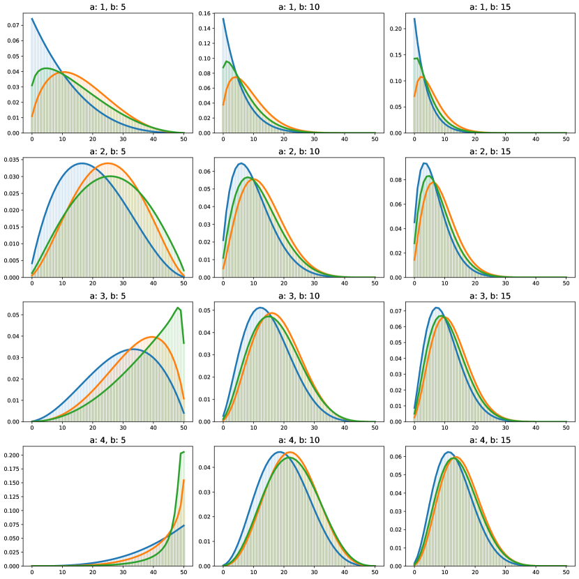
Figure 4: Posterior distribution of the empirical frequency level $f_{Y_{n+1,\ell}}$, assuming the Poisson setting with a Gamma CRM prior (blue line) and with a generalized Gamma CRM prior (orange and green lines). In all the panels, $a$ and $b$ vary, while we fix $c=50$, $m=1000$, $J=50$, $\theta=0.3$, $\tau=1$, $r=1$, and $\alpha=0.25,0.75$ for the orange and green lines respectively.

4 Discussion

This paper introduced a BNP approach to frequency recovery, both in the common “species" formulation and in a more general “traits" formulation of the problem. While the works Cai et al. [2018] and Dolera et al. [2021, 2023] applied BNPs to develop learning-augmented versions of the CMS under the DP and PYP priors, our approach is not built from the CMS, and considers the broad class of PK priors. For a PK prior, in Theorem 2.2 we provided the posterior distribution of the empirical frequency of a symbol $X_{n+1}$, given the sketch $\mathbf{C}_{J}$, which has been then applied to show peculiar properties of the DP and the PYP priors: i) Theorem 2.3 characterized the DP prior as the sole PK prior for which the posterior distribution depends on $\mathbf{C}_{J}$ only through $C_{h(X_{n+1})}$; ii) under the PYP prior, Theorem 2.4 identified a large sample regime to obtain an asymptotic approximation of the posterior distribution that depends on $\mathbf{C}_{J}$ only through $C_{h(X_{n+1})}$. The “traits" formulation of the frequency recovery problem is a further novelty with respect to Cai et al. [2018] and Dolera et al. [2021, 2023], and also with respect to the CMS literature, showing the flexibility of the BNP approach to deal with general data structures. In particular, for a CRM prior, in Theorem 3.3 we provided the posterior distribution of the empirical frequency level of a trait $Y_{n+1,\ell}$, given the sketch $\mathbf{C}_{J}$, showing how the Poisson process formulation of CRMs leads to a dependence of $\mathbf{C}_{J}$ only through $C_{h(Y_{n+1,\ell})}$. This result has been applied to the Poisson and Bernoulli distribution for the levels of associations of traits: i) Proposition 3.4 showed how, under the Gamma and generalized Gamma CRM priors, the Poisson distribution lead to simple posterior distributions; ii) for the Bernoulli distribution, Theorem 3.5 introduced a simple approximation of the posterior distribution.

Assuming the true data to be available, PK priors are widely used in BNPs, mostly for their mathematical tractability, leading to posterior inferences that are simple, computationally efficient and scalable to massive data sets [Lijoi and Prünster, 2010]. Our work shows how this desirable property of PK priors is no longer valid in BNP inference from sketched data, which poses additional challenges and constraints in the choice of the prior distribution. In particular, we showed how the PYP prior, which is arguably the most popular PK prior generalizing the DP, leads to a posterior distribution that is intractable to be evaluated, even for moderately large sample sizes. In general, our results show that the BNP approach to frequency recovery leads to non-trivial computational challenges in the evaluation of the posterior distribution under priors beyond a DP, which paves the way to: i) further investigating exact and approximate algorithms for an efficient (numerical) evaluation of the posterior distribution under the PYP prior; ii) further studying large sample approximations, possibly with (reliable) error bounds, of the posterior distribution under the PYP prior; iii) proposing different priors, with the aim of obtaining simple posterior distributions, while exhibiting more flexible tail behaviors than the DP. Differently from the “species" formulation of the frequency recovery problem, our results in the “traits" formulation show a much larger flexibility with respect to the choice of a prior distributions, leading to posterior distributions that are tractable to be evaluated for large sample sizes, at least assuming a Poisson distribution for the levels of associations of traits. Such a desirable property is determined by the Poisson process formulation of CRMs, which determines a posterior distribution that depends on the sketch $\mathbf{C}_{J}$ only through $C_{h(X_{n+1})}$.

By considering the “traits" formulation of the frequency recovery problem, we provided a further evidence of the flexibility of the BNP approach to deal with a broad range of discrete data structures. We argue that the BNP approach also allows for a great flexibility with respect to the object of interest, due to the use of the posterior distribution as the main tool to obtain estimates. For instance, our BNP approach may be extended to deal with more general quantities than the empirical frequency of a new data point, i.e. $f_{x_{n+1}}$. Of notable interest in the CMS literature is the problem of recovering the (cumulative) empirical frequency of $s\geq 1$ new data points [Cormode and Yi, 2020, Chapter 3]. To describe such a problem, it is useful to consider the “species" formulation of the frequency recovery problem. In particular, for $n\geq 1$ let $(x_{1},\ldots,x_{n})$ be a collection of $\mathbb{S}$-valued data points, and for a positive integer $J$ let $h:\mathbb{S}\rightarrow\{1,\ldots,J\}$ be a random hash function from the hash family $\mathcal{H}_{J}$. Assuming $(x_{1},\ldots,x_{n})$ to be available through the sketch $\mathbf{C}_{J}$, the goal is to recover the vector of empirical frequencies $(f_{x_{n+1}},\ldots,f_{x_{n+s}})$ of $s$ new data points $(x_{n+1},\ldots,x_{m+s})$ in $(x_{1},\ldots,x_{n})$, with the $r$-th empirical frequency $f_{x_{n+r}}$ being defined as $f_{x_{n+r}}=\sum_{1\leq i\leq n}I(x_{i}=x_{m+r})$, for $r=1,\ldots,s$. Then, the (cumulative) empirical frequency is obtained by summing the $f_{x_{n+r}}$’s. In principle, the arguments of Theorem 2.2 may be easily extended to provide the posterior distribution of $(f_{X_{n+1}},\ldots,f_{X_{n+s}})$, given $\mathbf{C}_{J}$ and the buckets in which the $X_{n+r}$’s are hashed, though we expect such a posterior distribution to have a rather complicated form, even under the DP prior. We refer to Dolera et al. [2023] for a discussion in the context of learning-augmented versions of the CMS.

Appendix A Proofs

A.1 Proof of 2.2

By the definition of conditional probability, we have that

$$\mathrm{Pr}\left[f_{X_{n+1}}=l\,|\,\bm{C}=\bm{c},h(X_{n+1})=j\right]=\frac{\mathrm{Pr}\left[f_{X_{n+1}}=l,\bm{C}=\bm{c},h(X_{n+1})=j\right]}{\mathrm{Pr}\left[\bm{C}=\bm{c},h(X_{n+1})=j\right]}$$ (22)

Let $g(t)=Z_{T}t^{-\gamma}e^{-\beta t}$, where $Z_{T}$ is a normalizing constant.

Denominator

We have

$$\mathrm{Pr}[\bm{C}=\bm{c},h(X_{n+1})=j]$$

$$\qquad=\binom{n}{c_{1},\ldots,c_{J}}\mathrm{Pr}\Big{[}X_{1}\in D_{j},\ldots,X_{c_{j}}\in D_{j},X_{n+1}\in D_{j},$$

$$\hskip 113.81102ptX_{i}\in D_{1},i\in[c_{j}:c_{j}+c_{1}],\ldots,X_{i}\in D_{j},i\in[\sum_{k=1}^{J-1}c_{k},n]\Big{]}$$

$$\qquad=\binom{n}{c_{1},\ldots,c_{J}}\mathds{E}\left[P(D_{j})^{c_{j}+1}\prod_{k\neq j}P(D_{k})^{c_{k}}\right]$$ (23)

From (23), writing $P(\cdot):=\tilde{\mu}(\cdot)/\tilde{\mu}(\mathbb{S})$ and the expression of $g(t)=g(\tilde{\mu}(\mathbb{S}))$

$$\mathrm{Pr}[\bm{C}=\bm{c},h(X_{n+1})=j]=\binom{n}{c_{1},\ldots,c_{j}}\mathds{E}\left[P(D_{j})^{c_{j}+1}\prod_{k\neq j}P(D_{k})^{c_{k}}\right]$$

$$\qquad=Z_{T}\binom{n}{c_{1},\ldots,c_{j}}\mathds{E}\left[\tilde{\mu}(\mathbb{S})^{-n-1-\gamma}e^{-\beta\tilde{\mu}(\mathbb{S})}\tilde{\mu}(D_{j})^{c_{j}+1}\prod_{k\neq j}\tilde{\mu}(D_{k})^{c_{k}}\right]$$

$$\qquad=Z_{T}\binom{n}{c_{1},\ldots,c_{j}}\int_{\mathbb{R}_{+}}\frac{u^{n+\gamma}}{\Gamma(n+\gamma+1)}\mathds{E}\left[e^{-(u+\beta)\tilde{\mu}(D_{j})}\tilde{\mu}(D_{j})^{c_{j}+1}\right]$$

$$\qquad\qquad\qquad\times\prod_{k\neq j}\mathds{E}\left[e^{-(u+\beta)\tilde{\mu}(D_{k})}\tilde{\mu}(D_{k})^{c_{k}}\right]$$

$$\qquad=Z_{T}\binom{n}{c_{1},\ldots,c_{j}}\int_{\mathbb{R}_{+}}\frac{u^{n+\gamma}}{\Gamma(n+\gamma+1)}(-1)^{c+1}\frac{\mathrm{d}^{c_{j}+1}}{\mathrm{d}z^{c_{j}+1}}e^{-\theta\psi(z)/J}|_{(u+\beta)}$$

$$\hskip 113.81102pt\prod_{k\neq j}(-1)^{c_{k}}\frac{\mathrm{d}^{c_{k}}}{\mathrm{d}z^{c_{k}}}e^{-\theta\psi(z)/J}|_{(u+\beta)}\mathrm{d}u$$

where the second equality follows from the definition of Poisson-Kingman model and the third one from the Gamma identity $\tilde{\mu}(\mathbb{S})^{-n-1-\gamma}=\int_{\mathbb{R}_{+}}u^{n+\gamma}/\Gamma(n+\gamma+1)e^{-u\tilde{\mu}(\mathbb{S})}\mathrm{d}x$, an application of Fubini’s theorem, and the independence property of CRMs. Finally the last equality follows from the properties of the exponential function and the definition of Laplace exponent of the CRM.

Numerator

Let $B_{\omega}$ denote a ball of radius $\varepsilon$ around $\omega\in\mathbb{S}$. We have

$$\mathrm{Pr}\left[\sum_{i=1}^{n}\mathrm{I}_{(X_{n+1})}(X_{i})=l,\bm{C}=\bm{c},h(X_{n+1})=j\right]=$$

$$\qquad\lim_{\varepsilon\rightarrow 0}\int_{D_{j}}\mathrm{Pr}\left[\sum_{i=1}^{n}\mathrm{I}_{B_{\omega^{*}}}(X_{i})=l,\bm{C}=\bm{C},X_{n+1}\in B_{\omega^{*}}\right]\mathrm{d}\omega^{*}$$

We consider the integrand,

$$\mathrm{Pr}\left[\sum_{i=1}^{n}\mathrm{I}_{B_{\omega^{*}}}(X_{i})=l,\sum_{i=1}^{n}\mathrm{I}_{h(\omega^{*})}(h(X_{i}))=c,X_{n+1}\in B_{\omega^{*}}\right]$$

$$\qquad=\binom{n}{l}\binom{n-l}{c_{1},\ldots,c_{j}-l,\ldots c_{J}}\mathrm{Pr}\Big{[}X_{1}\in B_{\omega^{*}}\ldots X_{l}\in B_{\omega^{*}},X_{n+1}\in B_{\omega^{*}},$$

$$\hskip 142.26378ptX_{l+1}\in D_{j}\setminus B_{\omega^{*}}\ldots,X_{c_{j}}\in D_{j}\setminus B_{\omega^{*}},$$

$$\hskip 142.26378ptX_{i}\in D_{1},i\in[c_{j}:c_{j}+c_{1}],\ldots,X_{i}\in D_{j},i\in[\sum_{l=1}^{J-1}c_{l},n]\Big{]}$$

$$\qquad=\frac{1}{l!}\binom{n}{c_{1},\ldots,c_{j}-l,\ldots c_{J}}\mathds{E}\left[P(B_{\omega^{*}})^{l+1}P(D_{j}\setminus B_{\omega^{*}})^{c_{j}-l}\prod_{k\neq j}P(D_{k})^{c_{k}}\right]$$ (24)

To evaluate the expected value, we proceed as in the case of the denominator and write

$$\mathds{E}\left[P(B_{\omega^{*}})^{l+1}P(D_{j}\setminus B_{\omega^{*}})^{c_{j}-l}\prod_{k\neq j}P(D_{k})^{c_{k}}\right]$$

$$\qquad=Z_{T}\int_{\mathbb{R}_{+}}\frac{u^{n+\gamma}}{\Gamma(n+\gamma+1)}\mathds{E}\left[e^{-(u+\beta)\tilde{\mu}(B_{\omega^{*}})}\tilde{\mu}(B_{\omega^{*}})^{l+1}\right]$$

$$\qquad\qquad\times\mathds{E}\left[e^{-(u+\beta)\tilde{\mu}(D_{j}\setminus B_{\omega^{*}})}\tilde{\mu}(D_{j}\setminus B_{\omega^{*}})^{c-l}\right]\prod_{k\neq j}\mathds{E}\left[e^{-(u+\beta)\tilde{\mu}(D_{k})}\tilde{\mu}(D_{k})^{c_{k}}\right]\mathrm{d}u$$

The two latter expected values above can be computed as in the denominator case. For the first expectation instead, letting $\varepsilon\rightarrow 0$ we have

$$\mathds{E}\left[e^{-(u+\beta)\tilde{\mu}(B_{\omega^{*}})}\tilde{\mu}(B_{\omega^{*}})^{l+1}\right]\rightarrow\kappa(u+\beta,l+1)\theta G_{0}(\mathrm{d}\omega^{*})$$

where $\kappa(u,l)=\int_{\mathbb{R}_{+}}s^{l}e^{-us}\rho(s)\mathrm{d}s$. This can be verified using, for instance, Lemma 1 in Camerlenghi et al. [2019]. Hence, the numerator equals

$$\mathrm{Pr}\left[\sum_{i=1}^{n}\mathrm{I}_{(X_{n+1})}(X_{i})=l,\bm{C}=\bm{c},h(X_{n+1})=j\right]$$

$$\qquad\frac{1}{l!}\binom{n}{c_{1},\ldots,c_{j}-l,\ldots c_{J}}\frac{Z_{T}}{\Gamma(n+\gamma+1)}$$

$$\hskip 56.9055pt\times\int_{D_{j}}\int_{\mathbb{R}_{+}}u^{n+\gamma}(-1)^{c_{j}-l}\left(\frac{\mathrm{d}^{c_{j}-l}}{\mathrm{d}(u+\beta)^{c_{j}-l}}e^{-\theta/J\psi(u+\beta)}\right)\times$$

$$\hskip 85.35826pt\times\prod_{k\neq j}(-1)^{c_{k}}\frac{\mathrm{d}^{c_{k}}}{\mathrm{d}z^{c_{k}}}e^{-\theta\psi(z)/J}|_{(u+\beta)}\kappa(u+\beta,l+1)\theta\mathrm{d}uG_{0}(\mathrm{d}\omega^{*})$$

where we can further integrate with respect to $\mathrm{d}\omega^{*}$ and observe $\int_{D_{j}}G_{0}(\mathrm{d}\omega^{*})=1/J$ thanks to the universality assumption on the hash function $h$. Combining numerator and denominator, and using the definition of $\phi^{(n)}(u)$, yields the result.

A.2 Proof of 2.3

Recalling the definition of $\psi^{(n)}(u)$, the claim of the theorem entails that

$$\frac{\int_{\mathbb{R}_{+}}u^{n+\gamma}\frac{\mathrm{d}^{c_{j}-l}}{\mathrm{d}(z)^{c_{j}-l}}e^{-\theta/J\psi(z)}|_{u+\beta}\prod_{k\neq j}\frac{\mathrm{d}^{c_{k}}}{\mathrm{d}z^{c_{k}}}e^{-\theta\psi(z)/J}|_{(u+\beta)}\kappa(u+\beta,l+1)\mathrm{d}u}{\int_{\mathbb{R}_{+}}u^{n+\gamma}\frac{\mathrm{d}^{c_{j}+1}}{\mathrm{d}z^{c_{j}+1}}e^{-\theta\psi(z)/J}|_{(u+\beta)}\prod_{k\neq j}\frac{\mathrm{d}^{c_{k}}}{\mathrm{d}z^{c_{k}}}e^{-\theta\psi(z)/J}|_{(u+\beta)}\mathrm{d}u}=f(n,c_{j},l)$$

where $f$ is an unknown function which cannot depend on $c_{k},k\neq j$. Then

$$\int_{\mathbb{R}_{+}}u^{n+\gamma}\frac{\mathrm{d}^{c_{j}-l}}{\mathrm{d}(z)^{c_{j}-l}}e^{-\theta/J\psi(z)}|_{u+\beta}\prod_{k\neq j}\frac{\mathrm{d}^{c_{k}}}{\mathrm{d}z^{c_{k}}}e^{-\theta\psi(z)/J}|_{(u+\beta)}\kappa(u+\beta,l+1)\mathrm{d}u=\\ f(n,c_{j},l)\int_{\mathbb{R}_{+}}u^{n+\gamma}\frac{\mathrm{d}^{c_{j}+1}}{\mathrm{d}z^{c_{j}+1}}e^{-\theta\psi(z)/J}|_{(u+\beta)}\prod_{k\neq j}\frac{\mathrm{d}^{c_{k}}}{\mathrm{d}z^{c_{k}}}e^{-\theta\psi(z)/J}|_{(u+\beta)}\mathrm{d}u$$

or equivalently

$$\int_{\mathbb{R}_{+}}u^{n+\gamma}\prod_{k\neq j}\frac{\mathrm{d}^{c_{k}}}{\mathrm{d}z^{c_{k}}}e^{-\theta\psi(z)/J}|_{(u+\beta)}\times\\ \left(\frac{\mathrm{d}^{c_{j}-l}}{\mathrm{d}(z)^{c_{j}-l}}e^{-\theta/J\psi(z)}|_{u+\beta}\kappa(u+\beta,l+1)-f(n,c_{j},l)\frac{\mathrm{d}^{c_{j}+1}}{\mathrm{d}z^{c_{j}+1}}e^{-\theta\psi(z)/J}|_{(u+\beta)}\right)\mathrm{d}u=0$$

Since the above equality must hold true for all values of $c_{k},k\neq j$, it is easy to see that

$$\frac{\mathrm{d}^{c_{j}-l}}{\mathrm{d}(z)^{c_{j}-l}}e^{-\theta/J\psi(z)}|_{u+\beta}\kappa(u+\beta,l+1)-f(n,c_{j},l)\frac{\mathrm{d}^{c_{j}+1}}{\mathrm{d}z^{c_{j}+1}}e^{-\theta\psi(z)/J}|_{(u+\beta)}\equiv 0$$ (25)

for all $u\geq 0$.

The simplest nontrivial case is when $c_{j}=1,l=0$ (indeed note that if $c_{j}=0$, $l=0$ by definition and we get $f(n,c_{j},l)=1$). Now, note that

$$\frac{\mathrm{d}}{\mathrm{d}z}e^{-\theta/J\psi(z)} =e^{-\theta/J\psi(z)}\left(-\frac{\theta}{J}\right)\frac{\mathrm{d}}{\mathrm{d}z}\psi(z)$$

$$\frac{\mathrm{d}^{2}}{\mathrm{d}z^{2}}e^{-\theta/J\psi(z)} =e^{-\theta/J\psi(z)}\left[\left(-\frac{\theta}{J}\right)\frac{\mathrm{d}}{\mathrm{d}z}\psi(z)\right]^{2}+e^{-\theta/J\psi(z)}\left(-\frac{\theta}{J}\right)\frac{\mathrm{d}^{2}}{\mathrm{d}z^{2}}\psi(z)$$

Plugging these into (25) we get

$$e^{-\theta/J\psi(u+\beta)}\Bigg{\{}-\frac{\theta}{J}\frac{\mathrm{d}}{\mathrm{d}z}\psi(z)|_{u+\beta}\kappa(u+\beta,1)+\\ -f(n,c_{j},l)\left(\left[\left(-\frac{\theta}{J}\right)\frac{\mathrm{d}}{\mathrm{d}z}\psi(z)\right]^{2}_{u+\beta}\right)-\frac{\theta}{J}\frac{\mathrm{d}^{2}}{\mathrm{d}z^{2}}\psi(z)|_{u+\beta}\Bigg{\}}=0$$

Given the positivity of the exponential function, we can set the term in the curly brackets equal to zero. Recalling that $\mathrm{d}/\mathrm{d}z\,\psi(z)=-\kappa(z,1)$, the term in the curly brackets above reduces to

$$\frac{\theta}{J}\kappa(u+\beta,1)^{2}-f(n,c_{j},l)\left(\frac{\theta^{2}}{J^{2}}\kappa(u+\beta,1)^{2}+\frac{\theta}{J}\frac{\mathrm{d}}{\mathrm{d}z}\kappa(z,1)|_{u+\beta}\right)=0$$

which entails

$$\frac{\mathrm{d}}{\mathrm{d}z}\kappa(z,1)=-\left(\frac{\theta}{J}-\frac{1}{f(m,c_{j},l)}\right)\kappa(z,1)^{2}.$$

Letting $w:=\left(\frac{\theta}{J}-\frac{1}{f(n,c_{j},l)}\right)^{-1}$, the differential equation above can be seen to have solution

$$\kappa(z,1)=\frac{1}{c+\frac{z}{w}}=\frac{w}{\tau+z}$$

where $c$ is an arbitrary constant and $\tau=cw$.

Let now $c_{j}=l=0$ and recall that in this case $f\equiv 1$. Plugging these into (25) we get

$$e^{-\theta/J\psi(u+\beta)}\kappa(u+\beta,1)-\frac{\mathrm{d}}{\mathrm{d}z}e^{-\theta/J\psi(z)} =0$$

which leads to

$$e^{-\theta/J\psi(u+\beta)}\left(\frac{w}{\tau+z}+\frac{\theta}{J}\frac{\mathrm{d}}{\mathrm{d}z}\psi(z)\right)_{|u+\beta}=0$$

Setting the term in the parentheses equal to zero, we obtain that

$$\psi(z)=K\log(\tau+z).$$ (26)

Hence, we have shown that if $\mathrm{Pr}\left[f_{X_{n+1}}=l\,|\,\bm{C}=\bm{c},h(X_{n+1})=j\right]$ does not depend on $c_{k}$, $k\neq j$, the CRM $\tilde{\mu}$ must have Lévy exponent (26).

Let now $\tilde{\mu}^{\prime}$ be a CRM with Lévy exponent $\psi$ as above. We first note that, without loss of generality, we can set $K=1$ since setting $K\neq 1$ the Laplace transform

$$\mathds{E}e^{-z\tilde{\mu}^{\prime}(A)}=e^{-K\log(\tau+z)\theta G_{0}(A)}=(\tau+z)^{-K\theta G_{0}(A)}=:F^{\prime}(z)$$

simply amounts to rescaling the total mass parameter.

We now show that $\tau$ must necessarily be equal to one. Note that if $\tilde{\mu}_{G}$ is a Gamma process, then its Lévy exponent is $\log(1+z)$, which is (26) but shifted of a term $(1-\tau)$:

$$\mathds{E}e^{-z\tilde{\mu}_{G}(A)}=(1+z)^{-K\theta G_{0}(A)}=F^{\prime}(z+(1-\tau))$$ (27)

Let $f_{A}$ be the probability density function of $\tilde{\mu}_{G}(A)$, and $f^{\prime}_{A}$ be the probability density function of $\tilde{\mu}^{\prime}(A)$. By the properties of the Laplace transform, (27) is equivalent to

$$f_{A}(t)=e^{(\tau-1)t}f^{\prime}_{A}(t),\quad\text{for all }t,$$

which is clearly impossible if $\tau\neq 1$ since we must have that both $f_{A}$ and $f^{\prime}_{A}$ must integrate to one since they are probability density functions. Hence, we have shown that if $\mathrm{Pr}\left[f_{X_{n+1}}=l\,|\,\bm{C}=\bm{c},h(X_{n+1})=j\right]$ does not depend on $c_{k},k\neq j$, the underlying CRM must be a Gamma process.

We are left with two degrees of freedom: namely the parameters $\gamma$ and $\beta$ defining the change of measure in the Poisson-Kingman model. However, note that if $\tilde{\mu}$ is a Gamma process, the resulting PK model with $g(t)\propto t^{-\gamma}e^{-\beta t}$ is still a Dirichlet process. This can be checked, for instance, starting from Eq. (177) in James [2002]. This concludes the proof.

A.3 Proof of Theorem 2.4

The proof relies on the use of an asymptotic property for a class of (normalized) generalized factorial coefficients. In particular, according to Dolera and Favaro [2020, Lemma 2], for any $z>0$ it holds

$$\lim_{n\rightarrow+\infty}\frac{z^{k}\mathscr{C}(n,k;s)}{\sum_{k=1}^{n}z^{k}\mathscr{C}(n,k;s)}=\text{e}^{-z}\frac{z^{k-1}}{(k-1)!}.$$ (28)

We start by rewriting the numerator and the denominator of the posterior distribution (7). With regards to the numerator of (7), we can write the following:

$$\frac{\gamma}{J}{c_{j}\choose l}(1-\alpha)_{(l)}$$ (29)

$$\quad\quad\times\sum_{i_{1}=1}^{c_{1}}J^{-i_{1}}\mathscr{C}(c_{1},i_{1};\alpha)\cdots\sum_{i_{j}=1}^{c_{j}-l}J^{-i_{j}}\mathscr{C}(c_{j}-l,i_{j};\alpha)\cdots\sum_{i_{J}=1}^{c_{J}}J^{-i_{J}}\mathscr{C}(c_{J},i_{J};\alpha)$$

$$\quad\quad\quad\times\Gamma\left(\frac{\gamma+\alpha}{\alpha}+i_{1}+\cdots+i_{j}+\cdots+i_{J}\right)$$

$$\frac{\gamma}{J}{c_{j}\choose l}(1-\alpha)_{(l)}\Gamma\left(\frac{\gamma+\alpha}{\alpha}\right)\left(\prod_{1\leq s\neq j\leq J}\sum_{i_{s}=1}^{c_{s}}\frac{1}{J^{i_{s}}}\mathscr{C}(c_{s},i_{s};\alpha)\right)$$

$$\quad\quad\times\sum_{i_{j}=1}^{c_{j}-l}\left(\frac{1}{J}\right)^{i_{j}}\mathscr{C}(c_{j}-l,i_{j};\alpha)\sum_{i_{1}=1}^{c_{1}}\left(\frac{\gamma+\alpha}{\alpha}\right)_{(i_{1})}\frac{\left(\frac{1}{J}\right)^{i_{1}}\mathscr{C}(c_{1},i_{1};\alpha)}{\sum_{i_{1}=1}^{c_{1}}\left(\frac{1}{J}\right)^{i_{1}}\mathscr{C}(c_{1},i_{1};\alpha)}\cdots$$

$$\quad\quad\quad\cdots\times\left(\frac{\gamma+\alpha}{\alpha}+i_{1}+\cdots+i_{j-1}\right)_{(i_{j})}\cdots$$

$$\quad\quad\quad\quad\cdots\times\sum_{i_{J}=1}^{c_{J}}\left(\frac{\gamma+\alpha}{\alpha}+i_{1}+\cdots+i_{J-1}\right)_{(i_{J})}\frac{\left(\frac{1}{J}\right)^{i_{J}}\mathscr{C}(c_{J},i_{J};\alpha)}{\sum_{i_{J}=1}^{c_{J}}\left(\frac{1}{J}\right)^{i_{J}}\mathscr{C}(c_{J},i_{J};\alpha)}.$$

By means of the same arguments, we can write the denominator of (7) as follows:

$$\sum_{i_{1}=1}^{c_{1}}J^{-i_{1}}\mathscr{C}(c_{1},i_{1};\alpha)\cdots\sum_{i_{j}=1}^{c_{j}+1}J^{-i_{j}}\mathscr{C}(c_{j}+1,i_{j};\alpha)\cdots\sum_{i_{J}=1}^{c_{J}}J^{-i_{J}}\mathscr{C}(c_{J},i_{J};\alpha)$$ (30)

$$\quad\times\Gamma\left(\frac{\gamma}{\alpha}+i_{1}+\cdots+i_{j}+\cdots+i_{J}\right)$$

$$\quad=\Gamma\left(\frac{\gamma}{\alpha}\right)\left(\prod_{1\leq s\neq j\leq J}\sum_{i_{s}=1}^{c_{s}}\frac{1}{J^{i_{s}}}\mathscr{C}(c_{s},i_{s};\alpha)\right)$$

$$\quad\quad\times\sum_{i_{j}=1}^{c_{j}+1}\left(\frac{1}{J}\right)^{i_{j}}\mathscr{C}(c_{j}+1,i_{j};\alpha)\sum_{i_{1}=1}^{c_{1}}\left(\frac{\gamma}{\alpha}\right)_{(i_{1})}\frac{\left(\frac{1}{J}\right)^{i_{1}}\mathscr{C}(c_{1},i_{1};\alpha)}{\sum_{i_{1}=1}^{c_{1}}\left(\frac{1}{J}\right)^{i_{1}}\mathscr{C}(c_{1},i_{1};\alpha)}\cdots$$

$$\quad\quad\quad\cdots\times\left(\frac{\gamma}{\alpha}+i_{1}+\cdots+i_{j-1}\right)_{(i_{j})}\cdots$$

$$\quad\quad\quad\quad\cdots\times\sum_{i_{J}=1}^{c_{J}}\left(\frac{\gamma}{\alpha}+i_{1}+\cdots+i_{J-1}\right)_{(i_{J})}\frac{\left(\frac{1}{J}\right)^{i_{J}}\mathscr{C}(c_{J},i_{J};\alpha)}{\sum_{i_{J}=1}^{c_{J}}\left(\frac{1}{J}\right)^{i_{J}}\mathscr{C}(c_{J},i_{J};\alpha)}.$$

Then, by combining the numerator (29) with the denominator (30), we can write the posterior distribution (7) as

$$\text{Pr}[f_{X_{n+1}}=l\,|\,\mathbf{C}_{J}=\mathbf{c},h(X_{n+1})=j]$$ (31)

$$\quad=\frac{\gamma}{J}{c_{j}\choose l}(1-\alpha)_{(l)}\frac{\Gamma\left(\frac{\gamma+\alpha}{\alpha}\right)}{\Gamma\left(\frac{\gamma}{\alpha}\right)}\frac{N_{\gamma,\alpha,J}(l;c_{1},\ldots,c_{J})}{D_{\gamma,\alpha,J}(c_{1},\ldots,c_{J})},$$

where

$$N_{\gamma,\alpha,J}(l;c_{1},\ldots,c_{J})$$ (32)

$$\quad=\sum_{i_{j}=1}^{c_{j}-l}\left(\frac{1}{J}\right)^{i_{j}}\mathscr{C}(c_{j}-l,i_{j};\alpha)\sum_{i_{1}=1}^{c_{1}}\left(\frac{\gamma+\alpha}{\alpha}\right)_{(i_{1})}\frac{\left(\frac{1}{J}\right)^{i_{1}}\mathscr{C}(c_{1},i_{1};\alpha)}{\sum_{i_{1}=1}^{c_{1}}\left(\frac{1}{J}\right)^{i_{1}}\mathscr{C}(c_{1},i_{1};\alpha)}\cdots$$

$$\quad\quad\cdots\times\left(\frac{\gamma+\alpha}{\alpha}+i_{1}+\cdots+i_{j-1}\right)_{(i_{j})}\cdots$$

$$\quad\quad\quad\cdots\times\sum_{i_{J}=1}^{c_{J}}\left(\frac{\gamma+\alpha}{\alpha}+i_{1}+\cdots+i_{J-1}\right)_{(i_{J})}\frac{\left(\frac{1}{J}\right)^{i_{J}}\mathscr{C}(c_{J},i_{J};\alpha)}{\sum_{i_{J}=1}^{c_{J}}\left(\frac{1}{J}\right)^{i_{J}}\mathscr{C}(c_{J},i_{J};\alpha)}$$

and

$$D_{\gamma,\alpha,J}(c_{1},\ldots,c_{J})$$ (33)

$$\quad=\sum_{i_{j}=1}^{c_{j}+1}\left(\frac{1}{J}\right)^{i_{j}}\mathscr{C}(c_{j}+1,i_{j};\alpha)\sum_{i_{1}=1}^{c_{1}}\left(\frac{\gamma}{\alpha}\right)_{(i_{1})}\frac{\left(\frac{1}{J}\right)^{i_{1}}\mathscr{C}(c_{1},i_{1};\alpha)}{\sum_{i_{1}=1}^{c_{1}}\left(\frac{1}{J}\right)^{i_{1}}\mathscr{C}(c_{1},i_{1};\alpha)}\cdots$$

$$\quad\quad\cdots\times\left(\frac{\gamma}{\alpha}+i_{1}+\cdots+i_{j-1}\right)_{(i_{j})}\cdots$$

$$\quad\quad\quad\cdots\times\sum_{i_{J}=1}^{c_{J}}\left(\frac{\gamma}{\alpha}+i_{1}+\cdots+i_{J-1}\right)_{(i_{J})}\frac{\left(\frac{1}{J}\right)^{i_{J}}\mathscr{C}(c_{J},i_{J};\alpha)}{\sum_{i_{J}=1}^{c_{J}}\left(\frac{1}{J}\right)^{i_{J}}\mathscr{C}(c_{J},i_{J};\alpha)}.$$

Now, we apply repeatedly (28) to both (32) and (33), starting from the last terms. In particular, for the summation in $i_{J}=1,\ldots,c_{J}$ of (32), we have that

$$\lim_{c_{J}\rightarrow+\infty}\sum_{i_{J}=1}^{c_{J}}\left(\frac{\gamma+\alpha}{\alpha}+i_{1}+\cdots+i_{J-1}\right)_{(i_{J})}\frac{\left(\frac{1}{J}\right)^{i_{J}}\mathscr{C}(c_{J},i_{J};\alpha)}{\sum_{i_{J}=1}^{c_{J}}\left(\frac{1}{J}\right)^{i_{J}}\mathscr{C}(c_{J},i_{J};\alpha)}$$ (34)

$$\quad=\sum_{i_{J}\geq 1}\left(\frac{\gamma+\alpha}{\alpha}+i_{1}+\cdots+i_{J-1}\right)_{(i_{J})}\text{e}^{-\frac{1}{J}}\frac{\left(\frac{1}{J}\right)^{i_{J}-1}}{(i_{J}-1)!}$$

$$\quad=\text{e}^{-\frac{1}{J}}\frac{\frac{\gamma+\alpha}{\alpha}+i_{1}+\cdots+i_{J-1}}{\left(1-\frac{1}{J}\right)^{\frac{\gamma+\alpha}{\alpha}+i_{1}+\cdots+i_{J-1}+1}},$$

and along the same arguments, for the summation in $i_{J}=1,\ldots,c_{J}$ of (33), we have

$$\lim_{c_{J}\rightarrow+\infty}\sum_{i_{J}=1}^{c_{J}}\left(\frac{\gamma}{\alpha}+i_{1}+\cdots+i_{J-1}\right)_{(i_{J})}\frac{\left(\frac{1}{J}\right)^{i_{J}}\mathscr{C}(c_{J},i_{J};\alpha)}{\sum_{i_{J}=1}^{c_{J}}\left(\frac{1}{J}\right)^{i_{J}}\mathscr{C}(c_{J},i_{J};\alpha)}$$ (35)

$$\quad=\sum_{i_{J}\geq 1}\left(\frac{\gamma}{\alpha}+i_{1}+\cdots+i_{J-1}\right)_{(i_{J})}\text{e}^{-\frac{1}{J}}\frac{\left(\frac{1}{J}\right)^{i_{J}-1}}{(i_{J}-1)!}$$

$$\quad=\text{e}^{-\frac{1}{J}}\frac{\frac{\gamma}{\alpha}+i_{1}+\cdots+i_{J-1}}{\left(1-\frac{1}{J}\right)^{\frac{\gamma}{\alpha}+i_{1}+\cdots+i_{J-1}+1}}.$$

Now, we consider the summation in $i_{J-1}=1,\ldots,c_{J-1}$ of (32), with (34), i.e.,

$$\lim_{c_{J-1}\rightarrow+\infty}\sum_{i_{J-1}=1}^{c_{J-1}}\left(\frac{\gamma+\alpha}{\alpha}+i_{1}+\cdots+i_{J-2}\right)_{(i_{J-1})}\text{e}^{-\frac{1}{J}}\frac{\frac{\gamma+\alpha}{\alpha}+i_{1}+\cdots+i_{J-1}}{\left(1-\frac{1}{J}\right)^{\frac{\gamma+\alpha}{\alpha}+i_{1}+\cdots+i_{J-1}+1}}$$

$$\quad\quad\times\frac{\left(\frac{1}{J}\right)^{i_{J-1}}\mathscr{C}(c_{J-1},i_{J-1};\alpha)}{\sum_{i_{J-1}=1}^{c_{J-1}}\left(\frac{1}{J}\right)^{i_{J-1}}\mathscr{C}(c_{J-1},i_{J-1};\alpha)}$$

$$\quad=\sum_{i_{J-1}\geq 1}\left(\frac{\gamma+\alpha}{\alpha}+i_{1}+\cdots+i_{J-2}\right)_{(i_{J-1})}\text{e}^{-\frac{1}{J}}\frac{\frac{\gamma+\alpha}{\alpha}+i_{1}+\cdots+i_{J-1}}{\left(1-\frac{1}{J}\right)^{\frac{\gamma+\alpha}{\alpha}+i_{1}+\cdots+i_{J-1}+1}}\text{e}^{-\frac{1}{J}}\frac{\left(\frac{1}{J}\right)^{i_{J-1}-1}}{(i_{J-1}-1)!}$$

$$\quad=\frac{\text{e}^{-\frac{2}{J}}}{\left(1-\frac{1}{J}\right)^{\frac{\gamma+\alpha}{\alpha}+i_{1}+\cdots+i_{J-2}+2}}\sum_{i_{J-1}\geq 1}\left(\frac{\gamma+\alpha}{\alpha}+i_{1}+\cdots+i_{J-2}\right)_{(i_{J-1}+1)}\frac{\left(\frac{1}{J-1}\right)^{i_{J-1}-1}}{(i_{J-1}-1)!}$$

$$\quad=\frac{\text{e}^{-\frac{2}{J}}}{\left(1-\frac{1}{J}\right)^{\frac{\gamma+\alpha}{\alpha}+i_{1}+\cdots+i_{J-2}+2}}\frac{\left(\frac{\gamma+\alpha}{\alpha}+i_{1}+\cdots+i_{J-2}\right)_{(2)}}{\left(\frac{J-2}{J-1}\right)^{\frac{\gamma+\alpha}{\alpha}+i_{1}+\cdots+i_{J-2}+2}}$$

$$\quad=\text{e}^{-\frac{2}{J}}\frac{\left(\frac{\gamma+\alpha}{\alpha}+i_{1}+\cdots+i_{J-2}\right)_{(2)}}{\left(1-\frac{2}{J}\right)^{\frac{\gamma+\alpha}{\alpha}+i_{1}+\cdots+i_{J-2}+2}}.$$

Similarly, consider the summation in $i_{J-1}=1,\ldots,c_{J-1}$ of (33), with (35), i.e.,

$$\lim_{c_{J-1}\rightarrow+\infty}\sum_{i_{J-1}=1}^{c_{J-1}}\left(\frac{\gamma}{\alpha}+i_{1}+\cdots+i_{J-2}\right)_{(i_{J-1})}\text{e}^{-\frac{1}{J}}\frac{\frac{\gamma}{\alpha}+i_{1}+\cdots+i_{J-1}}{\left(1-\frac{1}{J}\right)^{\frac{\gamma}{\alpha}+i_{1}+\cdots+i_{J-1}+1}}$$

$$\quad\quad\times\frac{\left(\frac{1}{J}\right)^{i_{J-1}}\mathscr{C}(c_{J-1},i_{J-1};\alpha)}{\sum_{i_{J-1}=1}^{c_{J-1}}\left(\frac{1}{J}\right)^{i_{J-1}}\mathscr{C}(c_{J-1},i_{J-1};\alpha)}$$

$$\quad=\sum_{i_{J-1}\geq 1}\left(\frac{\gamma}{\alpha}+i_{1}+\cdots+i_{J-2}\right)_{(i_{J-1})}\text{e}^{-\frac{1}{J}}\frac{\frac{\gamma}{\alpha}+i_{1}+\cdots+i_{J-1}}{\left(1-\frac{1}{J}\right)^{\frac{\gamma}{\alpha}+i_{1}+\cdots+i_{J-1}+1}}\text{e}^{-\frac{1}{J}}\frac{\left(\frac{1}{J}\right)^{i_{J-1}-1}}{(i_{J-1}-1)!}$$

$$\quad=\frac{\text{e}^{-\frac{2}{J}}}{\left(1-\frac{1}{J}\right)^{\frac{\gamma}{\alpha}+i_{1}+\cdots+i_{J-2}+2}}\sum_{i_{J-1}\geq 1}\left(\frac{\gamma}{\alpha}+i_{1}+\cdots+i_{J-2}\right)_{(i_{J-1}+1)}\frac{\left(\frac{1}{J-1}\right)^{i_{J-1}-1}}{(i_{J-1}-1)!}$$

$$\quad=\frac{\text{e}^{-\frac{2}{J}}}{\left(1-\frac{1}{J}\right)^{\frac{\gamma}{\alpha}+i_{1}+\cdots+i_{J-2}+2}}\frac{\left(\frac{\gamma}{\alpha}+i_{1}+\cdots+i_{J-2}\right)_{(2)}}{\left(\frac{J-2}{J-1}\right)^{\frac{\gamma}{\alpha}+i_{1}+\cdots+i_{J-2}+2}}$$

$$\quad=\text{e}^{-\frac{2}{J}}\frac{\left(\frac{\gamma}{\alpha}+i_{1}+\cdots+i_{J-2}\right)_{(2)}}{\left(1-\frac{2}{J}\right)^{\frac{\gamma}{\alpha}+i_{1}+\cdots+i_{J-2}+2}}.$$

By proceeding recursively, for the summation in $i_{j+1}=1,\ldots,c_{j+1}$ of (32) is such that

$$\lim_{c_{j+1}\rightarrow+\infty}\sum_{i_{j+1}=1}^{c_{j+1}}\left(\frac{\gamma+\alpha}{\alpha}+i_{1}+\cdots+i_{j}\right)_{(i_{j+1})}\text{e}^{-\frac{J-j-1}{J}}\frac{\left(\frac{\gamma+\alpha}{\alpha}+i_{1}+\cdots+i_{j+1}\right)_{(J-j-1)}}{\left(1-\frac{J-j-1}{J}\right)^{\frac{\gamma+\alpha}{\alpha}+i_{1}+\cdots+i_{j+1}+J-j-1}}$$ (36)

$$\quad\quad\times\frac{\left(\frac{1}{J}\right)^{i_{j+1}}\mathscr{C}(c_{j+1},i_{j+1};\alpha)}{\sum_{i_{j+1}=1}^{c_{j+1}}\left(\frac{1}{J}\right)^{i_{j+1}}\mathscr{C}(c_{j+1},i_{j+1};\alpha)}$$

$$\quad=\sum_{c_{j+1}\geq 1}\left(\frac{\gamma+\alpha}{\alpha}+i_{1}+\cdots+i_{j}\right)_{(i_{j+1})}\text{e}^{-\frac{J-j-1}{J}}\frac{\left(\frac{\gamma+\alpha}{\alpha}+i_{1}+\cdots+i_{j+1}\right)_{(J-j-1)}}{\left(1-\frac{J-j-1}{J}\right)^{\frac{\gamma+\alpha}{\alpha}+i_{1}+\cdots+i_{j+1}+J-j-1}}\text{e}^{-\frac{1}{J}}\frac{\left(\frac{1}{J}\right)^{i_{j+1}-1}}{(i_{j+1}-1)!}$$

$$\quad=\frac{\text{e}^{-\frac{J-j}{J}}}{\left(1-\frac{J-j-1}{J}\right)^{\frac{\gamma+\alpha}{\alpha}+i_{1}+\cdots+i_{j}+J-j}}\sum_{i_{j+1}\geq 1}\left(\frac{\gamma+\alpha}{\alpha}+i_{1}+\cdots+i_{j}\right)_{(i_{j+1}+J-j-1)}\frac{\left(\frac{1}{j+1}\right)^{i_{j+1}-1}}{(i_{j+1}-1)!}$$

$$\quad=\frac{\text{e}^{-\frac{J-j}{J}}}{\left(1-\frac{J-j-1}{J}\right)^{\frac{\gamma+\alpha}{\alpha}+i_{1}+\cdots+i_{j}+J-j}}\frac{\left(\frac{\gamma+\alpha}{\alpha}+i_{1}+\cdots+i_{j}\right)_{(J-j)}}{\left(\frac{j}{j+1}\right)^{\frac{\gamma+\alpha}{\alpha}+i_{1}+\cdots+i_{j}+J-j}}$$

$$\quad=\text{e}^{-\frac{J-j}{J}}\frac{\left(\frac{\gamma+\alpha}{\alpha}+i_{1}+\cdots+i_{j}\right)_{(J-j)}}{\left(1-\frac{J-j}{J}\right)^{\frac{\gamma+\alpha}{\alpha}+i_{1}+\cdots+i_{j}+J-j}},$$

and, along the same lines, the summation in $i_{j+1}=1,\ldots,c_{j+1}$ of (33) is such that

$$\lim_{c_{j+1}\rightarrow+\infty}\sum_{i_{j+1}=1}^{c_{j+1}}\left(\frac{\gamma}{\alpha}+i_{1}+\cdots+i_{j}\right)_{(i_{j+1})}\text{e}^{-\frac{J-j-1}{J}}\frac{\left(\frac{\gamma}{\alpha}+i_{1}+\cdots+i_{j+1}\right)_{(J-j-1)}}{\left(1-\frac{J-j-1}{J}\right)^{\frac{\gamma}{\alpha}+i_{1}+\cdots+i_{j+1}+J-j-1}}$$ (37)

$$\quad\quad\times\frac{\left(\frac{1}{J}\right)^{i_{j+1}}\mathscr{C}(c_{j+1},i_{j+1};\alpha)}{\sum_{i_{j+1}=1}^{c_{j+1}}\left(\frac{1}{J}\right)^{i_{j+1}}\mathscr{C}(c_{j+1},i_{j+1};\alpha)}$$

$$\quad=\sum_{c_{j+1}\geq 1}\left(\frac{\gamma}{\alpha}+i_{1}+\cdots+i_{j}\right)_{(i_{j+1})}\text{e}^{-\frac{J-j-1}{J}}\frac{\left(\frac{\gamma}{\alpha}+i_{1}+\cdots+i_{j+1}\right)_{(J-j-1)}}{\left(1-\frac{J-j-1}{J}\right)^{\frac{\gamma}{\alpha}+i_{1}+\cdots+i_{j+1}+J-j-1}}\text{e}^{-\frac{1}{J}}\frac{\left(\frac{1}{J}\right)^{i_{j+1}-1}}{(i_{j+1}-1)!}$$

$$\quad=\frac{\text{e}^{-\frac{J-j}{J}}}{\left(1-\frac{J-j-1}{J}\right)^{\frac{\gamma}{\alpha}+i_{1}+\cdots+i_{j}+J-j}}\sum_{i_{j+1}\geq 1}\left(\frac{\gamma}{\alpha}+i_{1}+\cdots+i_{j}\right)_{(i_{j+1}+J-j-1)}\frac{\left(\frac{1}{j+1}\right)^{i_{j+1}-1}}{(i_{j+1}-1)!}$$

$$\quad=\frac{\text{e}^{-\frac{J-j}{J}}}{\left(1-\frac{J-j-1}{J}\right)^{\frac{\gamma}{\alpha}+i_{1}+\cdots+i_{j}+J-j}}\frac{\left(\frac{\gamma}{\alpha}+i_{1}+\cdots+i_{j}\right)_{(J-j)}}{\left(\frac{j}{j+1}\right)^{\frac{\gamma}{\alpha}+i_{1}+\cdots+i_{j}+J-j}}$$

$$\quad=\text{e}^{-\frac{J-j}{J}}\frac{\left(\frac{\gamma}{\alpha}+i_{1}+\cdots+i_{j}\right)_{(J-j)}}{\left(1-\frac{J-j}{J}\right)^{\frac{\gamma}{\alpha}+i_{1}+\cdots+i_{j}+J-j}}$$

Now, we consider the summation in $i_{j-1}=1,\ldots,c_{j-1}$ of (32), with (36), i.e.,

$$\lim_{c_{j-1}\rightarrow+\infty}\sum_{i_{j-1}=1}^{c_{j-1}}\left(\frac{\gamma+\alpha}{\alpha}+i_{1}+\cdots+i_{j-2}\right)_{(i_{j-1})}\left(\frac{\gamma+\alpha}{\alpha}+i_{1}+\cdots+i_{j-1}\right)_{(i_{j})}$$

$$\quad\quad\times\text{e}^{-\frac{J-j}{J}}\frac{\left(\frac{\gamma+\alpha}{\alpha}+i_{1}+\cdots+i_{j}\right)_{(J-j)}}{\left(1-\frac{J-j}{J}\right)^{\frac{\gamma+\alpha}{\alpha}+i_{1}+\cdots+i_{j}+J-j}}\frac{\left(\frac{1}{J}\right)^{i_{j-1}}\mathscr{C}(c_{j-1},i_{j-1};\alpha)}{\sum_{i_{j-1}=1}^{c_{j-1}}\left(\frac{1}{J}\right)^{i_{j-1}}\mathscr{C}(c_{j-1},i_{j-1};\alpha)}$$

$$\quad=\sum_{i_{j-1}\geq 1}\left(\frac{\gamma+\alpha}{\alpha}+i_{1}+\cdots+i_{j-2}\right)_{(i_{j-1})}\left(\frac{\gamma+\alpha}{\alpha}+i_{1}+\cdots+i_{j-1}\right)_{(i_{j})}$$

$$\quad\quad\times\text{e}^{-\frac{J-j}{J}}\frac{\left(\frac{\gamma+\alpha}{\alpha}+i_{1}+\cdots+i_{j}\right)_{(J-j)}}{\left(1-\frac{J-j}{J}\right)^{\frac{\gamma+\alpha}{\alpha}+i_{1}+\cdots+i_{j}+J-j}}\text{e}^{-\frac{1}{J}}\frac{\left(\frac{1}{J}\right)^{i_{j-1}-1}}{(i_{j-1}-1)!}$$

$$\quad=\frac{\text{e}^{-\frac{J-j+1}{J}}}{\left(1-\frac{J-j}{J}\right)^{\frac{\gamma+\alpha}{\alpha}+i_{j}+i_{1}+\cdots+i_{j-2}+J-j+1}}\sum_{i_{j-1}\geq 1}\left(\frac{\gamma+\alpha}{\alpha}+i_{1}+\cdots+i_{j-2}\right)_{(i_{j-1}+i_{j}+J-j)}\frac{\left(\frac{1}{j}\right)^{i_{j-1}-1}}{(i_{j-1}-1)!}$$

$$\quad=\frac{\text{e}^{-\frac{J-j+1}{J}}}{\left(1-\frac{J-j}{J}\right)^{\frac{\gamma+\alpha}{\alpha}+i_{j}+i_{1}+\cdots+i_{j-2}+J-j+1}}\frac{\left(\frac{\gamma+\alpha}{\alpha}+i_{1}+\cdots+i_{j-2}\right)_{(i_{j}+J-j+1)}}{\left(\frac{j-1}{j}\right)^{\frac{\gamma+\alpha}{\gamma}+i_{j}+i_{1}+\cdots+i_{j-2}+J-j+1}}$$

$$\quad=\text{e}^{-\frac{J-j+1}{J}}\frac{\left(\frac{\gamma+\alpha}{\alpha}+i_{1}+\cdots+i_{j-2}\right)_{(i_{j}+J-j+1)}}{\left(\frac{j-1}{J}\right)^{\frac{\gamma+\alpha}{\gamma}+i_{j}+i_{1}+\cdots+i_{j-2}+J-j+1}}.$$

Similarly, consider the summation in $i_{j-1}=1,\ldots,c_{j-1}$ of (33), with (37), i.e.,

$$\lim_{c_{j-1}\rightarrow+\infty}\sum_{i_{j-1}=1}^{c_{j-1}}\left(\frac{\gamma}{\alpha}+i_{1}+\cdots+i_{j-2}\right)_{(i_{j-1})}\left(\frac{\gamma}{\alpha}+i_{1}+\cdots+i_{j-1}\right)_{(i_{j})}$$

$$\quad\quad\times\text{e}^{-\frac{J-j}{J}}\frac{\left(\frac{\gamma}{\alpha}+i_{1}+\cdots+i_{j}\right)_{(J-j)}}{\left(1-\frac{J-j}{J}\right)^{\frac{\gamma}{\alpha}+i_{1}+\cdots+i_{j}+J-j}}\frac{\left(\frac{1}{J}\right)^{i_{j-1}}\mathscr{C}(c_{j-1},i_{j-1};\alpha)}{\sum_{i_{j-1}=1}^{c_{j-1}}\left(\frac{1}{J}\right)^{i_{j-1}}\mathscr{C}(c_{j-1},i_{j-1};\alpha)}$$

$$\quad=\sum_{i_{j-1}\geq 1}\left(\frac{\gamma}{\alpha}+i_{1}+\cdots+i_{j-2}\right)_{(i_{j-1})}\left(\frac{\gamma}{\alpha}+i_{1}+\cdots+i_{j-1}\right)_{(i_{j})}$$

$$\quad\quad\times\text{e}^{-\frac{J-j}{J}}\frac{\left(\frac{\gamma}{\alpha}+i_{1}+\cdots+i_{j}\right)_{(J-j)}}{\left(1-\frac{J-j}{J}\right)^{\frac{\gamma}{\alpha}+i_{1}+\cdots+i_{j}+J-j}}\text{e}^{-\frac{1}{J}}\frac{\left(\frac{1}{J}\right)^{i_{j-1}-1}}{(i_{j-1}-1)!}$$

$$\quad=\frac{\text{e}^{-\frac{J-j+1}{J}}}{\left(1-\frac{J-j}{J}\right)^{\frac{\gamma}{\alpha}+i_{j}+i_{1}+\cdots+i_{j-2}+J-j+1}}\sum_{i_{j-1}\geq 1}\left(\frac{\gamma}{\alpha}+i_{1}+\cdots+i_{j-2}\right)_{(i_{j-1}+i_{j}+J-j)}\frac{\left(\frac{1}{j}\right)^{i_{j-1}-1}}{(i_{j-1}-1)!}$$

$$\quad=\frac{\text{e}^{-\frac{J-j+1}{J}}}{\left(1-\frac{J-j}{J}\right)^{\frac{\gamma}{\alpha}+i_{j}+i_{1}+\cdots+i_{j-2}+J-j+1}}\frac{\left(\frac{\gamma}{\alpha}+i_{1}+\cdots+i_{j-2}\right)_{(i_{j}+J-j+1)}}{\left(\frac{j-1}{j}\right)^{\frac{\gamma}{\gamma}+i_{j}+i_{1}+\cdots+i_{j-2}+J-j+1}}$$

$$\quad=\text{e}^{-\frac{J-j+1}{J}}\frac{\left(\frac{\gamma}{\alpha}+i_{1}+\cdots+i_{j-2}\right)_{(i_{j}+J-j+1)}}{\left(\frac{j-1}{J}\right)^{\frac{\gamma}{\gamma}+i_{j}+i_{1}+\cdots+i_{j-2}+J-j+1}}.$$

By proceeding recursively, we arrive to the summation in $i_{1}=1,\ldots,c_{1}$ of (32), i.e.

$$\lim_{c_{1}\rightarrow+\infty}\sum_{i_{1}=1}^{c_{1}}\left(\frac{\gamma+\alpha}{\alpha}\right)_{(i_{1})}\text{e}^{-\frac{J-2}{J}}\frac{\left(\frac{\gamma+\alpha}{\alpha}+i_{1}\right)_{(i_{j}+J-2)}}{\left(\frac{2}{J}\right)^{\frac{\gamma+\alpha}{\alpha}+i_{j}+i_{1}+J-2}}\frac{\left(\frac{1}{J}\right)^{i_{1}}\mathscr{C}(c_{1},i_{1};\alpha)}{\sum_{i_{1}=1}^{c_{1}}\left(\frac{1}{J}\right)^{i_{1}}\mathscr{C}(c_{1},i_{1};\alpha)}$$ (39)

$$\quad=\sum_{i_{1}\geq 1}\left(\frac{\gamma+\alpha}{\alpha}\right)_{(i_{1})}\text{e}^{-\frac{J-2}{J}}\frac{\left(\frac{\gamma+\alpha}{\alpha}+i_{1}\right)_{(i_{j}+J-2)}}{\left(\frac{2}{J}\right)^{\frac{\gamma+\alpha}{\alpha}+i_{j}+i_{1}+J-2}}\text{e}^{-\frac{1}{J}}\frac{\left(\frac{1}{J}\right)^{i_{1}-1}}{(i_{1}-1)!}$$

$$\quad=\frac{\text{e}^{-\frac{J-1}{J}}}{\left(\frac{2}{J}\right)^{\frac{\gamma+\alpha}{\alpha}+i_{j}+J-1}}\sum_{i_{1}\geq 1}\left(\frac{\gamma+\alpha}{\alpha}\right)_{(i_{1}+i_{j}+J-2)}\frac{\left(\frac{1}{2}\right)^{i_{1}-1}}{(i_{1}-1)!}$$

$$\quad=\frac{\text{e}^{-\frac{J-1}{J}}}{\left(\frac{2}{J}\right)^{\frac{\gamma+\alpha}{\alpha}+i_{j}+J-1}}\frac{\left(\frac{\gamma+\alpha}{\alpha}\right)_{(i_{j}+J-1)}}{\left(\frac{1}{2}\right)^{\frac{\gamma+\alpha}{\alpha}+i_{j}+J-1}}$$

$$\quad=\text{e}^{-\frac{J-1}{J}}\frac{\left(\frac{\gamma+\alpha}{\alpha}\right)_{(i_{j}+J-1)}}{\left(\frac{1}{J}\right)^{\frac{\gamma+\alpha}{\alpha}+i_{j}+J-1}}$$

and, along the same lines, we arrive to the summation in $i_{1}=1,\ldots,c_{1}$ of (33), i.e.

$$\lim_{c_{1}\rightarrow+\infty}\sum_{i_{1}=1}^{c_{1}}\left(\frac{\gamma}{\alpha}\right)_{(i_{1})}\text{e}^{-\frac{J-2}{J}}\frac{\left(\frac{\gamma}{\alpha}+i_{1}\right)_{(i_{j}+J-2)}}{\left(\frac{2}{J}\right)^{\frac{\gamma}{\alpha}+i_{j}+i_{1}+J-2}}\frac{\left(\frac{1}{J}\right)^{i_{1}}\mathscr{C}(c_{1},i_{1};\alpha)}{\sum_{i_{1}=1}^{c_{1}}\left(\frac{1}{J}\right)^{i_{1}}\mathscr{C}(c_{1},i_{1};\alpha)}$$ (40)

$$\quad=\sum_{i_{1}\geq 1}\left(\frac{\gamma}{\alpha}\right)_{(i_{1})}\text{e}^{-\frac{J-2}{J}}\frac{\left(\frac{\gamma}{\alpha}+i_{1}\right)_{(i_{j}+J-2)}}{\left(\frac{2}{J}\right)^{\frac{\gamma}{\alpha}+i_{j}+i_{1}+J-2}}\text{e}^{-\frac{1}{J}}\frac{\left(\frac{1}{J}\right)^{i_{1}-1}}{(i_{1}-1)!}$$

$$\quad=\frac{\text{e}^{-\frac{J-1}{J}}}{\left(\frac{2}{J}\right)^{\frac{\gamma}{\alpha}+i_{j}+J-1}}\sum_{i_{1}\geq 1}\left(\frac{\gamma}{\alpha}\right)_{(i_{1}+i_{j}+J-2)}\frac{\left(\frac{1}{2}\right)^{i_{1}-1}}{(i_{1}-1)!}$$

$$\quad=\frac{\text{e}^{-\frac{J-1}{J}}}{\left(\frac{2}{J}\right)^{\frac{\gamma}{\alpha}+i_{j}+J-1}}\frac{\left(\frac{\gamma}{\alpha}\right)_{(i_{j}+J-1)}}{\left(\frac{1}{2}\right)^{\frac{\gamma}{\alpha}+i_{j}+J-1}}$$

$$\quad=\text{e}^{-\frac{J-1}{J}}\frac{\left(\frac{\gamma}{\alpha}\right)_{(i_{j}+J-1)}}{\left(\frac{1}{J}\right)^{\frac{\gamma}{\alpha}+i_{j}+J-1}}.$$

We $\mathbf{c}_{-j}=(c_{1},\ldots,c_{j-1},c_{j+1},\ldots,c_{J})$ and indicate by $\mathbf{c}_{-j}\rightarrow+\infty$ the limit situation when $c_{k}\rightarrow+\infty$ simultaneously for $k\neq j$ while $c_{j}$ is fixed. Then, according to the asymptotics obtained in (39) and (40), from (31) we can write

$$\lim_{\mathbf{c}_{-j}\rightarrow+\infty}\frac{\gamma}{J}{c_{j}\choose l}(1-\alpha)_{(l)}\frac{\Gamma\left(\frac{\gamma+\alpha}{\alpha}\right)}{\Gamma\left(\frac{\gamma}{\alpha}\right)}\frac{N_{\gamma,\alpha,J}(l;c_{1},\ldots,c_{J})}{D_{\gamma,\alpha,J}(c_{1},\ldots,c_{J})}$$

$$\quad=\frac{\gamma}{J}{c_{j}\choose l}(1-\alpha)_{(l)}\frac{\Gamma\left(\frac{\gamma+\alpha}{\alpha}\right)}{\Gamma\left(\frac{\gamma}{\alpha}\right)}\frac{\sum_{i_{j}=1}^{c_{j}-l}\left(\frac{1}{J}\right)^{i_{j}}\mathscr{C}(c_{j}-l,i_{j};\alpha)\text{e}^{-\frac{J-1}{J}}\frac{\left(\frac{\gamma+\alpha}{\alpha}\right)_{(i_{j}+J-1)}}{\left(\frac{1}{J}\right)^{\frac{\gamma+\alpha}{\alpha}+i_{j}+J-1}}}{\sum_{i_{j}=1}^{c_{j}+1}\left(\frac{1}{J}\right)^{i_{j}}\mathscr{C}(c_{j}+1,i_{j};\alpha)\text{e}^{-\frac{J-1}{J}}\frac{\left(\frac{\gamma}{\alpha}\right)_{(i_{j}+J-1)}}{\left(\frac{1}{J}\right)^{\frac{\gamma}{\alpha}+i_{j}+J-1}}}$$

$$\quad=\gamma{c_{j}\choose l}(1-\alpha)_{(l)}\frac{\Gamma\left(\frac{\gamma+\alpha}{\alpha}\right)}{\Gamma\left(\frac{\gamma}{\alpha}\right)}\frac{\sum_{i_{j}=1}^{c_{j}-l}\mathscr{C}(c_{j}-l,i_{j};\alpha)\left(\frac{\gamma+\alpha}{\alpha}\right)_{(i_{j}+J-1)}}{\sum_{i_{j}=1}^{c_{j}+1}\mathscr{C}(c_{j}+1,i_{j};\alpha)\left(\frac{\gamma}{\alpha}\right)_{(i_{j}+J-1)}}$$

$$\quad=\gamma{c_{j}\choose l}(1-\alpha)_{(l)}\frac{\Gamma\left(\frac{\gamma+\alpha}{\alpha}+J-1\right)}{\Gamma\left(\frac{\gamma}{\alpha}+J-1\right)}\frac{\sum_{i_{j}=1}^{c_{j}-l}\mathscr{C}(c_{j}-l,i_{j};\alpha)\left(\frac{\gamma+\alpha}{\alpha}+J-1\right)_{(i_{j})}}{\sum_{i_{j}=1}^{c_{j}+1}\mathscr{C}(c_{j}+1,i_{j};\alpha)\left(\frac{\gamma}{\alpha}+J-1\right)_{(i_{j})}}$$

$$\quad=\gamma{c_{j}\choose l}(1-\alpha)_{(l)}\frac{\Gamma\left(\frac{\gamma+\alpha}{\alpha}+J-1\right)}{\Gamma\left(\frac{\gamma}{\alpha}+J-1\right)}\frac{(\gamma+\alpha+J\alpha-\alpha)_{(c_{j}-l)}}{(\gamma+J\alpha-\alpha)_{(c_{j}+1)}},$$

where the summations over $i_{j}$ follows from Equation 2.49 in Charalambides [2005]. See also Charalambides [2005, Theorem 2.14]. This completes the proof.

A.4 Proof of 3.2

Without loss of generality, assume that $A_{i,k}\in\mathbb{N}_{0}:=\{0,1,\ldots\}$. From the Poisson process representation of CRMs and the marking theorem [Kingman, 1993], $\tilde{N}:=\{(\omega_{k},J_{k},(A_{i,k})_{i=1}^{n+1})\}_{k\geq 1}$ is a Poisson process on $\mathbb{S}\times\mathbb{R}_{+}\times\mathbb{N}_{0}^{n+1}$. Consider now thinned processes $\tilde{N}_{j}$, $j=1,\ldots,J$ obtained from $\tilde{N}$ by taking only those points for which $\omega_{k}\in D_{j}$. By the coloring theorem [Kingman, 1993], the $\tilde{N}_{j}$’s are independent Poisson processes.

Now observe that the random variables $f_{Y_{n+1,\ell}}$, $X_{n+1}(Y_{n+1,\ell})$ depend only on $\tilde{N}_{h(Y_{n+1,\ell})}$. Similarly, each $(C_{j},B{j})$ depends only on $\tilde{N}_{j}$ and the independence is preserved also when marginalizing the $\tilde{N}_{j}$’s. Hence, we can conclude that $(f_{Y_{n+1,\ell}}$, $X_{n+1}(Y_{\ell}),C_{h(Y_{n+1,\ell})},B_{h(Y_{\ell})})$ are independent of all the other $C_{k}$’s ($k\neq h(Y_{\ell})$) and all of $B_{k}$ ($k\neq h(Y_{\ell})$), which yields the proof.

A.5 Proof of Theorem 3.3

We evaluate (14) by computing the numerator and denominator separately. In the following, we will denote by $D_{\omega}$ the preimage of $h(\omega)$, for $\omega\in\mathbb{S}$.

Denominator

From the Poisson process representation of CRMs and the marking theorem, we have that $N:=\left\{(\omega_{k},S_{k},\{A_{i,k}\}_{i=1}^{n+1}\right\}_{k\geq 1}$ is a Poisson process on $\mathbb{S}\times\mathbb{R}_{+}\times\mathbb{N}^{n+1}$ with intensity

$$\theta G_{0}(\mathrm{d}w)\left[\prod_{i=1}^{n+1}G_{A}(\mathrm{d}a_{i}\,|\,s)\right]\rho(s)\mathrm{d}s$$

Then by the colouring theorem [see, e.g., Chapter 5 in Kingman, 1993], we have that selecting from $N$ only those points for which $\omega_{k}\in D_{j}$ (i.e., the points whose features’ hashes coincide with the hash of $Y_{n+1,\ell}$), leads to a point process $N^{\prime}:=\left\{(\omega^{\prime}_{k},S^{\prime}_{k},\{A^{\prime}_{i,k}\}_{i=1}^{n+1}\right\}_{k\geq 1}$ which is Poisson on $D_{j}\times\mathbb{R}_{+}\times\mathbb{N}^{n+1}$ with intensity

$$\frac{\theta}{J}\bar{G}_{j}(\mathrm{d}w)\left[\prod_{i=1}^{n+1}G_{A}(\mathrm{d}a_{i}\,|\,s)\right]\rho(s)\mathrm{d}s$$ (41)

where $\bar{G}_{j}(\mathrm{d}w)$ is $G_{0}$ truncated on $D_{\omega^{*}}$ and re-normalized. Then,

$$\mathrm{Pr}\left[C_{j}=c,B_{j}=b\right]=$$

$$\qquad=\mathrm{Pr}\left[\sum_{k\geq 1}\mathrm{I}[\omega_{k}\in D_{\omega^{*}}]\sum_{i=1}^{n}A_{i,k}=c,\sum_{k\geq 1}\mathrm{I}[\omega_{k}\in D_{\omega^{*}}]A_{i,n+1}=b\right]$$

$$\qquad=\mathrm{Pr}\left[\sum_{k\geq 1}\sum_{i=1}^{m}A^{\prime}_{i,k}=c,\sum_{k\geq 1}A^{\prime}_{n+1,k}=b\right]$$

Observe that $\omega_{k}$ is not involved in the last probability, so we can marginalize with respect to it and consider the point process $\{J^{\prime}_{k},(A^{\prime}_{i,k})_{i=1}^{n+1}\}_{k\geq 1}$ on $\mathbb{R}_{+}\times\mathbb{N}_{0}^{n+1}$ with intensity $\theta J^{-1}\left[\prod_{i=1}^{n+1}G_{A}(\mathrm{d}a_{i}\,|\,s)\right]\rho(s)\mathrm{d}s$.

Numerator

We start by considering $Y_{n+1,\ell}=\omega^{*}$ fixed. Let $B_{\omega^{*}}$ be a ball of radius $\varepsilon$ centered in $\omega^{*}$. We compute

$$\mathrm{Pr}\left[\sum_{i=1}^{n}X_{i}(B_{\omega^{*}})=l,X_{n+1}(B_{\omega^{*}})=a,C_{j}=c,B_{j}=b,h(\omega^{*})=j\right]$$

which converges to the numerator in (14) as $\varepsilon\rightarrow 0$. By the definition of $B_{j}$ and $C_{j}$ we have

$$\mathrm{Pr}\left[\sum_{i=1}^{n}X_{i}(B_{\omega^{*}})=l,X_{n+1}(B_{\omega^{*}})=a,C_{j}=c,B_{j}=b\right]$$ (42)

$$\qquad=\mathrm{Pr}\Big{[}\sum_{i=1}^{n}X_{i}(B_{\omega^{*}})=l,X_{n+1}(B_{\omega^{*}})=a,$$

$$\hskip 28.45274pt\sum_{i=1}^{n}X_{i}(D_{\omega^{*}}\setminus B_{\omega^{*}})=(c-l),X_{n+1}(D_{\omega^{*}}\setminus B_{\omega^{*}})=(b-a)\Big{]}$$

We further have that $(X_{i}(B_{\omega^{*}}))_{i\geq 1}$ is a collection of random variables independent of $(X_{i}(D_{\omega^{*}}\setminus B_{\omega^{*}}))_{i\geq 1}$. Therefore, we can consider the first two events and the last two events separately.

For the last two, arguing as in the denominator case, we have that as $\varepsilon\rightarrow 0$

$$\mathrm{Pr}\Big{[}\sum_{i=1}^{n}X_{i}(D_{\omega^{*}}\setminus B_{\omega^{*}})=(c-l),X_{n+1}(D_{\omega^{*}}\setminus B_{\omega^{*}})=(b-a)\Big{]}\\ \longrightarrow\mathrm{Pr}\left[\sum_{k\geq 1}\sum_{i=1}^{n}A^{\prime}_{i,k}=c-l,\sum_{k\geq 1}A^{\prime}_{n+1,k}=b-a\right]$$

where the $A^{\prime}_{ik}$’s come from the Poisson process $\{J^{\prime}_{k},(A^{\prime}_{i,k})_{i=1}^{n+1}\}_{k\geq 1}$ on $\mathbb{R}_{+}\times\mathbb{N}_{0}^{n+1}$ with intensity $\theta J^{-1}\left[\prod_{i=1}^{n+1}G_{A}(\mathrm{d}a_{i}\,|\,s)\right]\rho(s)\mathrm{d}s$.

For the first two events instead, an application of Campbell’s theorem yields

$$\mathrm{Pr}\Big{[}\sum_{i=1}^{n}X_{i}(B_{\omega^{*}})=l,X_{n+1}(B_{\omega^{*}})=a\Big{]}$$

$$\qquad=\mathds{E}\left[\int I\left[\left\{\sum_{i=1}^{n}a_{i}\right\}=l\right]I[a_{n+1}=a]I[\omega\in B_{\omega^{*}}]N(\mathrm{d}s\,\mathrm{d}\bm{a}\,\mathrm{d}\omega)\right]$$

$$\qquad=\theta G_{0}(B_{\omega^{*}})\int\mathrm{Pr}\left[\sum_{i=1}^{n}\tilde{A}_{i}=l,\tilde{A}_{n+1}=a\,|\,s\right]\rho(s)\mathrm{d}s$$

The proof concludes by letting $\varepsilon\rightarrow 0$ and noting that $\int_{D_{j}}G_{0}(\mathrm{d}\omega^{*})=J^{-1}$.

A.6 Proof of 3.4

The closeness of the Poisson distribution under convolution entails that $\sum_{i=1}^{n}\tilde{A}_{i}\,|\,s\sim\mbox{Poi}(nrs)$. Similarly, $\sum_{k\geq 1}\sum_{i=1}^{n}A^{\prime}_{i,k}\sim\mbox{Poi}(nrT^{\prime})$ where $T^{\prime}=\sum_{k\geq 1}J^{\prime}_{k}$. Then

$$\int_{\mathbb{R}_{+}}\mathrm{Pr}\left[\sum_{i=1}^{n}\tilde{A}_{i}=l,\tilde{A}_{n+1}=a\,|\,s\right]\rho(s)\mathrm{d}s$$

$$\qquad\qquad=\int_{\mathbb{R}_{+}}\frac{1}{l!}\frac{1}{a!}(nrs)^{l}e^{-nrs}(rs)^{a}e^{-rs}\rho(s)\mathrm{d}s$$

$$\qquad\qquad=\frac{n^{l}r^{l+a}}{l!a!}\kappa(l+a,(n+1)r).$$

Moreover

$$\mathrm{Pr}\left[\sum_{k\geq 1}\sum_{i=1}^{n}A^{\prime}_{i,k}=c,\sum_{k\geq 1}A^{\prime}_{n+1,k}=b\right]$$

$$\qquad\qquad=\frac{n^{c}r^{c+b}}{c!b!}\mathds{E}_{T^{\prime}}\left[e^{-(n+1)rT^{\prime}}(T^{\prime})^{c+b}\right]$$

$$\qquad\qquad=\frac{n^{c}r^{c+b}}{c!b!}(-1)^{c+b}\frac{\mathrm{d}^{c+b}}{\mathrm{d}((n+1)r)^{c+b}}\mathds{E}_{\mu^{\prime}}[e^{-(n+1)rT^{\prime}}]$$

$$\qquad\qquad=\frac{n^{c}r^{c+b}}{c!b!}(-1)^{c+b}\frac{\mathrm{d}^{c+b}}{\mathrm{d}z^{c+b}}\exp\left(-\theta/J\psi(z)\right)\big{|}_{(n+1)r}$$

In a similar fashion,

$$\mathrm{Pr}\left[\sum_{k\geq 1}\sum_{i=1}^{n}A^{\prime}_{i,k}=c-l,\sum_{k\geq 1}A^{\prime}_{n+1,k}=b-a\right]$$ (43)

$$\qquad\qquad\frac{n^{c-l}r^{c-l+b-a}}{(c-l)!(b-a)!}(-1)^{c-l+b-a}\frac{\mathrm{d}^{c-l+b-a}}{\mathrm{d}z^{c-l+b-a}}\exp\left(-\theta/J\psi(z)\right)\big{|}_{(n+1)r}$$

Combining these expressions together yields the proof.

A.7 Proof of 3.5

Observe that $(J^{\prime}_{k})_{k\geq 1}$ in 3.3 is a Poisson process on $\mathbb{R}_{+}$ with intensity $\theta/J\rho(s)\mathrm{d}s$. Consider now the numerator in (15). Let $S_{n}:=\sum_{k\geq 1}\sum_{i=1}^{n}A^{\prime}_{i,k}$ and $Z:=\sum_{k\geq 1}A^{\prime}_{n+1,k}$. We have that, conditionally to $(J^{\prime}_{k})_{k\geq 1}$, $S_{n,k}$ is Poisson-binomial distributed with paramterers $J^{\prime}_{1},\ldots,J^{\prime}_{1},J^{\prime}_{2},\ldots,J^{\prime}_{2},\ldots$, where each $J^{\prime}_{k}$ appears exactly $n$ times. Similarly, $Z\,|\,(J^{\prime}_{k})_{k\geq 1}$ is Poisson-binomial with parameters $J_{1},J_{2},\ldots$. Let $\tilde{S}_{n}\,|\,(J^{\prime}_{k})_{k\geq 1}\sim\mbox{Poi}(nT^{\prime})$ and $\tilde{Z}\,|\,(J^{\prime}_{k})_{k\geq 1}\sim\mbox{Poi}(T^{\prime})$ where $T^{\prime}=\sum_{k}J^{\prime}_{k}$. Then, by Le Cam [1960], conditionally to $(J^{\prime}_{k})_{k\geq 1}$, $S_{n}\approx\tilde{S}_{n}$, $Z\approx\tilde{Z}$. Hence

$$\mathrm{Pr}[S_{n}=c-l,Z=b-1]\approx\mathrm{Pr}[\tilde{S}_{n}=c-l,\tilde{Z}=b-1]$$

Then, from (43) we get

$$\mathrm{Pr}[\tilde{S}_{n}=c-l,\tilde{Z}=b-1]=\\ \frac{n^{c-l}r^{c-l+b-1}}{(c-l)!(b-1)!}(-1)^{c-l+b-1}\frac{\mathrm{d}^{c-l+b-1}}{\mathrm{d}z^{c-l+b-1}}\exp\left(-\theta/J\psi(z)\right)\big{|}_{(n+1)r}.$$

Moreover,

$$\mathrm{Pr}\left[\sum_{i=1}^{n}\tilde{A}_{i}=l,\tilde{A}_{n+1}=1\,|\,s\right]$$

$$\qquad=\binom{n}{l}\mathrm{Pr}[\tilde{A}_{1}=1,\ldots,\tilde{A}_{l}=1,\tilde{A}_{n+1}=1,\tilde{A}_{l+1}=0,\ldots,\tilde{A}_{n}=0]$$

$$\qquad=\binom{n}{l}s^{n+1}(1-s)^{m-l}=\binom{n}{l}\left(s^{l+1}-s^{n+1}\right)$$

Integrating the resulting expression with respect to $\rho(s)\mathrm{d}s$ and ignoring multiplicative terms yields (15).

To prove the error bound, for ease of notation, let $f_{Y}\equiv f_{Y_{n+1,\ell}}$, $X\equiv X_{n+1}(Y_{n+1,\ell})$ and let $M^{\prime}=(J_{k})_{k\geq 1}$. Furthermore, observe that $(f_{Y},X)$ is independent of $(S_{n},Z)$ and $(\tilde{S}_{n},\tilde{Z})$. Then

$$TV\left(\left[f_{Y},X,S_{n},Z\right],\left[f_{Y},X,\tilde{S}_{n},\tilde{Z}\right]\right)$$

$$\quad=\sum_{l,x,s,z}\Big{|}\mathrm{Pr}\left[f_{Y}=l,X=x,S_{n}=s,Z=z\right]-\mathrm{Pr}\left[f_{Y}=l,X=x,\tilde{S}_{n}=s,\tilde{Z}=z\right]\Big{|}$$

$$\quad=\sum_{l,x,s,z}\mathrm{Pr}\left[f_{Y}=l,X=x\right]\Big{|}\mathrm{Pr}\left[S_{n}=s,Z=z\right]-\mathrm{Pr}\left[\tilde{S}_{n}=s,\tilde{Z}=z\right]\Big{|}$$

$$\quad\leq\sum_{s,z}\Big{|}\mathds{E}\mathrm{Pr}\left[S_{n}=s,Z=z\,|\,M^{\prime}\right]-\mathds{E}\mathrm{Pr}\left[\tilde{S}_{n}=s,\tilde{Z}=z\,|\,M^{\prime}\right]\Big{|}$$

$$\quad\leq\mathds{E}\sum_{s,z}\Big{|}\mathrm{Pr}\left[S_{n}=s,Z=z\,|\,M^{\prime}\right]-\mathrm{Pr}\left[\tilde{S}_{n}=s,\tilde{Z}=z\,|\,M^{\prime}\right]\Big{|}$$

where the last inequality follows from Jensen’s inequality and an application of the Fubini theorem. Then by the conditional independence between $S_{n}$ and $Z$, and $\tilde{S}_{n}$ and $\tilde{Z}$ we get

$$\mathds{E}\sum_{s,z}\Big{|}\mathrm{Pr}\left[S_{n}=s,Z=z\,|\,M^{\prime}\right]-\mathrm{Pr}\left[\tilde{S}_{n}=s,\tilde{Z}=z\,|\,M^{\prime}\right]\Big{|}$$

$$\qquad=\mathds{E}\left[TV(S_{n}\,|\,M^{\prime},\tilde{S}_{n}\,|\,M^{\prime})+TV(Z\,|\,M^{\prime},\tilde{Z}\,|\,M^{\prime})\right]$$

To upper bound the error, we start from Eq. (5.5) in Steele [1994] so that

$$TV(S_{n}\,|\,M^{\prime},\tilde{S}_{n}\,|\,M^{\prime}) \leq\frac{(1-e^{-nT^{\prime}})}{nT^{\prime}}n\sum_{k\geq 1}J_{k}^{\prime 2}$$

$$TV(Z\,|\,M^{\prime},\tilde{Z}\,|\,M^{\prime}) \leq\frac{(1-e^{-T^{\prime}})}{T^{\prime}}\sum_{k\geq 1}J_{k}^{\prime 2}$$

so that

$$\mathds{E}\left[TV(S_{n}\,|\,M^{\prime},\tilde{S}_{n}\,|\,M^{\prime})+TV(Z\,|\,M^{\prime},\tilde{Z}\,|\,M^{\prime})\right]$$

$$\qquad\leq\mathds{E}\left[\frac{2}{T^{\prime}}\sum_{k\geq 1}J_{k}^{\prime 2}\right]=2\int_{\mathbb{R}_{+}}\mathds{E}\left[e^{-uT^{\prime}}\sum_{k\geq 1}J_{k}^{\prime 2}\right]\mathrm{d}u$$

$$\qquad=2\int_{\mathbb{R}_{+}}\mathds{E}\left[\int_{\mathbb{R}_{+}}e^{-u\int_{\mathbb{R}_{+}}zM^{\prime}(\mathrm{d}z)}s^{2}M^{\prime}(\mathrm{d}z)\right]\mathrm{d}u$$

where the last equality follows by identifying $M^{\prime}$ with the random counting measure $\sum_{k\geq 1}\delta_{J^{\prime}_{k}}$. Then, an application of the Mecke equation [see, e.g., Theorem 4.1 in Last and Penrose, 2018] yields

$$2\int_{\mathbb{R}_{+}}\mathds{E}\left[\int_{\mathbb{R}_{+}}e^{-u\int_{\mathbb{R}_{+}}zM^{\prime}(\mathrm{d}z)}s^{2}M^{\prime}(\mathrm{d}z)\right]\mathrm{d}u=$$

$$\qquad=\frac{2\theta}{J}\int_{\mathbb{R}_{+}}\int_{\mathbb{R}_{+}}\mathds{E}[e^{-uT^{\prime}}]e^{-us}s^{2}\rho(s)\mathrm{d}s.$$

The proof follows by noticing that, by the Lévy-Kintchine representation, $\mathds{E}[e^{-uT^{\prime}}]=e^{-\psi(u)}$ and from the definition of $\kappa(u,n)$.

Appendix B Details about the Dirichlet Process case

B.1 Proof of Equation (5) as a special case

The DP is obtained by normalizing a Gamma process, whose Lévy intensity is $\theta s^{-1}e^{-s}\mathrm{d}sG_{0}(\mathrm{d}x)$. Hence,

$$\psi(u) =\int_{\mathbb{R}_{+}}(1-e^{-us})\rho(s)\mathrm{d}s=\int_{\mathbb{R}_{+}}(1-e^{-us})s^{-1}e^{-s}\mathrm{d}s$$

$$=\int_{\mathbb{R}_{+}}\int_{\mathbb{R}_{+}}(1-e^{-us})e^{-ts}e^{-s}\mathrm{d}t\,\mathrm{d}s$$

$$=\int_{\mathbb{R}_{+}}\frac{u}{(t+1)(t+u+1)}\mathrm{d}t=\log(1+u)$$

where the third equality follows from the identity $s^{-1}=\int_{\mathbb{R}_{+}}e^{-ts}\mathrm{d}t$ and the fourth one by an application of Fubini’s theorem. Then it follows

$$(-1)^{n}\frac{\mathrm{d}^{u}}{\mathrm{d}u^{n}}e^{-\theta\psi(u)}=\frac{\Gamma(\theta+n)}{\Gamma(\theta)}(1+u)^{-\theta-n},$$

Moreover, $k(l,u)=\Gamma(l)/(u+1)^{l}$. Hence, the integral at the numerator of (4) can be evaluated as

$$\frac{\Gamma(\theta/J+c_{j}-l)}{\Gamma(\theta/J)}\prod_{k\neq j}\frac{\Gamma(\theta/J+c_{k})}{\Gamma(\theta/J)}\Gamma(l+1)\int_{\mathbb{R}_{+}}u^{n}+(1+u)^{-\theta-n-1}$$

$$\qquad=\frac{\Gamma(\theta/J+c_{j}-l)}{\Gamma(\theta/J)}\prod_{k\neq j}\frac{\Gamma(\theta/J+c_{k})}{\Gamma(\theta/J)}\Gamma(l+1)\frac{\Gamma(n+1)}{\Gamma(\theta+n+1)}$$

Similarly, the integral at the denominator of (4) equals

$$\frac{\Gamma(\theta/J+c_{j}+1)}{\Gamma(\theta/J)}\prod_{k\neq j}\frac{\Gamma(\theta/J+c_{k})}{\Gamma(\theta/J)}\int_{\mathbb{R}_{+}}u^{n}+(1+u)^{-\theta-n-1}$$

$$\qquad=\frac{\Gamma(\theta/J+c_{j}+1)}{\Gamma(\theta/J)}\prod_{k\neq j}\frac{\Gamma(\theta/J+c_{k})}{\Gamma(\theta/J)}\frac{\Gamma(n+1)}{\Gamma(\theta+n+1)}$$

Combining these expressions together, we have

$$\mathrm{Pr}\left[f_{X_{n+1}}=l\,|\,\bm{C}=\bm{c},h(X_{n+1})=j\right]=\frac{\theta}{J}\binom{c_{j}}{l}l!\frac{\Gamma(\theta/J+c_{j}-l)}{\Gamma(\theta/J+c_{j}+1)}.$$

B.2 Proof of Equation (5) from the finite dimensional laws

In this proof, we exploit only the original characterization of the DP in terms of its finite-dimensional distributions. That is, given $\theta>0$ and $G_{0}$ a probability measure on $(\mathbb{S})$, $P$ is a Dirichlet process with mean measure $\theta G_{0}$ if and only if, for any $n>0$ and any $n$ measurable partition $A_{1},\ldots,A_{n}$ of $\mathbb{X}$,

$$(P(A_{1}),\ldots,P(A_{n}))\sim\mathrm{Dir}_{n}(\theta G_{0}(A_{1}),\ldots,\theta G_{0}(A_{n}))$$ (44)

where $\mathrm{Dir}_{n}$ denotes the $n-1$ dimensional Dirichlet distribution.

We argue as in Section A.1. To compute the denominator in (22), from (23), (44)

$$\mathrm{Pr}[\bm{C}=\bm{c},h(X_{n+1})=j]$$

$$\qquad=\binom{n}{c_{1},\ldots,c_{J}}\frac{\Gamma(\theta)}{\Gamma(\theta+n+1)}\frac{\Gamma(\theta/J+c_{j}+1)}{\Gamma(\theta/J)}\prod_{k\neq j}\frac{\Gamma(\theta/J+c_{k})}{\Gamma(\theta/J)}$$

where we also exploited the e uniformity of the hash function which ensures that $G_{0}(D_{\ell})=G_{0}(h^{-1}(\{\ell\}))=1/J$ for any $\ell=1,\ldots,J$.

Similarly, to compute the numerator, consider (24). Since $P$ is a Dirichlet process,

$$\mathds{E}\left[P(B_{\omega^{*}})^{l+1}P(D_{j}\setminus B_{\omega^{*}})^{c_{j}-l}\prod_{k\neq j}P(D_{k})^{c_{k}}\right]$$

$$\qquad=\frac{1}{l!}\binom{n}{c_{1},\ldots,c_{j}-l,\ldots c_{J}}\frac{\Gamma(\theta)}{\Gamma(\theta+n+1)}\frac{\Gamma(\alpha G_{0}(B_{\omega^{*}})+l+1)}{\Gamma(\theta G_{0}(B_{\omega^{*}}))}$$

$$\qquad\qquad\times\frac{\Gamma(\theta G_{0}(D_{j}\setminus B_{\omega^{*}})+c_{j}-l)}{\Gamma(\theta G_{0}(D_{j}\setminus B_{\omega^{*}}))}\prod_{k\neq j}\frac{\Gamma(\theta/J+c_{k})}{\Gamma(\theta/J)}$$

We now let $\varepsilon\rightarrow 0$. First note that, of course

$$\frac{\Gamma(\theta G_{0}(D_{j}\setminus B_{\omega^{*}})+c_{j}-l)}{\Gamma(\theta G_{0}(D_{j}\setminus B_{\omega^{*}}))}\rightarrow\frac{\Gamma(\theta G_{0}(D_{j})+c_{j}-l)}{\Gamma(\theta G_{0}(D_{j}))}=\frac{\Gamma(\theta/J+c_{j}-l)}{\Gamma(\theta/J)}$$

To evaluate the limit of $\Gamma(\theta G_{0}(B_{\omega^{*}})+l+1)/\Gamma(\theta G_{0}(B_{\omega^{*}}))$, we first unroll the numerator using the recurrence relation $\Gamma(z+1)=z\Gamma(z)$ $l$ times so that

$$\frac{\Gamma(\theta G_{0}(B_{\omega^{*}})+l+1)}{\Gamma(\theta G_{0}(B_{\omega^{*}}))}=(\theta G_{0}(B_{\omega^{*}})+l)\cdots(\theta G_{0}(B_{\omega^{*}}))=\theta\Gamma(l+1)G_{0}(B_{\omega^{*}})+o(G_{0}(B_{\omega^{*}}))$$

letting now $\varepsilon\rightarrow 0$, we can ignore higher order infinitesimals and get that

$$\frac{\Gamma(\theta G_{0}(B_{\omega^{*}})+l+1)}{\Gamma(\theta G_{0}(B_{\omega^{*}}))}\rightarrow\theta\Gamma(l+1)G_{0}(\mathrm{d}\omega^{*}),$$

which leads to

$$\mathrm{Pr}\left[\sum_{i=1}^{n}\mathrm{I}_{(X_{n+1})}(X_{i})=l,\bm{C}=\bm{c},h(X_{n+1})=j\right]$$

$$\qquad=\int_{D_{j}}\mathrm{Pr}\left[\sum_{i=1}^{n}\mathrm{I}_{X_{n+1}}(X_{i})=l,\bm{C}=\bm{c},X_{n+1}\in\mathrm{d}\omega^{*}\right]$$

$$\qquad=\frac{1}{l!}\binom{n}{c_{1},\ldots,c_{j}-l,\ldots c_{J}}\frac{\Gamma(\theta)}{\Gamma(\theta+n+1)}\theta\Gamma(l+1)G_{0}(B_{\omega^{*}})$$

$$\qquad\qquad\times\frac{\Gamma(\theta/J+c_{j}-l)}{\Gamma(\theta/J)}\prod_{k\neq j}\frac{\Gamma(\theta/J+c_{k})}{\Gamma(\theta/J)}\int_{D_{j}}G_{0}(\mathrm{d}\omega^{*})$$

So that integration with respect to $\mathrm{d}\omega^{*}$ is now straightforward and $\int_{D_{j}}G_{0}(\mathrm{d}\omega^{*})=1/J$.

Combining numerator and denominator yields the proof.

Appendix C Details About the PYP Case

C.1 Proof of (7)

In the case of a PYP, we have $\beta=0$, $\psi(u)=u^{\alpha}$ and

$$\kappa(u,l)=\alpha u^{\alpha-l}\frac{\Gamma(l-\alpha)}{\Gamma(1-\alpha)}=\alpha u^{\alpha-l}(1-\alpha)_{(l-1)}$$

where $(a)_{(b)}$ is the $b$-th rising factoral, i.e. $(a)_{(b)}=a(a+1)\cdots(a+b-1)$. Using the Faa di Bruno formula, we further have [see, e.g., Lemma 1 in Camerlenghi et al., 2019]

$$(-1)^{c}\frac{\mathrm{d}^{c}}{\mathrm{d}u^{c}}e^{-u^{\alpha}/J} =e^{-u^{\alpha}/J}\sum_{i=1}^{c}\left(\frac{1}{J}\right)^{i}\sum_{(*)}\frac{1}{i!}\binom{c}{k_{1}\cdots k_{i}}\prod_{j=1}^{i}\kappa(u,k_{j})$$

$$=e^{-u^{\alpha}/J}\sum_{i=1}^{c}\left(\frac{1}{J}\right)^{i}\frac{\alpha^{i}}{u^{c-\alpha i}i!}\sum_{(*)}\binom{c}{k_{1}\cdots k_{i}}\prod_{j=1}^{i}(1-\alpha)_{k_{j}-1}$$

$$=e^{-u^{\alpha}/J}\sum_{i=1}^{c}\left(\frac{1}{J}\right)^{i}\frac{1}{u^{c-\alpha i}}\mathscr{C}(c,i;\alpha)$$

where $\mathscr{C}(c,i;\alpha)$ is the generalized factorial coefficient and $(*)$ denotes the summation over positive integers $(k_{1},\ldots,k_{i})$ such that $\sum_{j=1}^{i}k_{j}=c$.

Recall the definition of the multi-index set $S(\bm{c},j,q)$ as in the main text below (7). Then, the integral at the numerator of (4) equals

$$\int_{\mathbb{R}_{+}}u^{b+\gamma}e^{-u^{\alpha}/J}\sum_{i_{j}=1}^{c_{j}-l}J^{-i_{j}}\frac{\mathscr{C}(c_{j}-l,i_{j};\alpha)}{u^{c_{j}-l-\alpha i_{j}}}$$

$$\hskip 56.9055pt\times\Bigg{\{}\prod_{k\neq j}e^{-u^{\alpha}/J}\sum_{i_{k}=1}^{c_{k}}J^{-i_{k}}\frac{\mathscr{C}(c_{k},i_{k};\alpha)}{u^{c_{k}-\alpha i_{k}}}\Bigg{\}}\alpha u^{\alpha-l-1}(1-\alpha)_{(l)}\mathrm{d}u$$

$$=\sum_{i_{1}=1}^{c_{1}}\cdots\sum_{i_{j}=1}^{c_{j}-l}\cdots\sum_{i_{J}=1}^{c_{J}}J^{-\sum_{k}i_{k}}\mathscr{C}(c_{j}-l,i_{j};\alpha)$$

$$\hskip 56.9055pt\times\prod_{k\neq j}\mathscr{C}(c_{k},i_{k};\alpha)\alpha(1-\alpha)_{(l)}\int_{\mathbb{R}_{+}}e^{-u^{\alpha}}u^{\gamma-1+\alpha\sum_{k}i_{k}+\alpha}\mathrm{d}u$$

$$=\sum_{i_{1}=1}^{c_{1}}\cdots\sum_{i_{j}=1}^{c_{j}-l}\cdots\sum_{i_{J}=1}^{c_{J}}J^{-\sum_{k}i_{k}}\mathscr{C}(c_{j}-l,i_{j};\alpha)$$

$$\hskip 56.9055pt\times\prod_{k\neq j}\mathscr{C}(c_{k},i_{k};\alpha)(1-\alpha)_{(l)}\Gamma\left(\frac{\gamma+\alpha}{\alpha}+\sum_{k}i_{k}\right)$$

$$=(1-\alpha)_{(l)}\sum_{\bm{i}\in\mathcal{S}(\bm{c},j,-l)}\Gamma\left(\frac{\gamma+\alpha}{\alpha}+|\bm{i}|\right)J^{-|\bm{i}|}\prod_{k=1}^{J}\mathscr{C}(c_{k}-l\delta_{k,j},i_{k};\alpha).$$

Similarly, the integral at the denominator of (4) equals

$$\sum_{i_{1}=1}^{c_{1}}\cdots\sum_{i_{j}=1}^{c_{j}+1}\cdots\sum_{i_{J}=1}^{c_{J}}J^{-\sum_{k}i_{k}}\mathscr{C}(c_{j}+1,i_{j};\alpha)\prod_{k\neq j}\mathscr{C}(c_{k},i_{k};\alpha)\Gamma\left(\frac{\gamma}{\alpha}+\sum_{k}i_{k}\right)$$

$$=\sum_{\bm{i}\in\mathcal{S}(\bm{c},j,1)}\Gamma\left(\gamma/\alpha+|\bm{i}|\right)J^{-|\bm{i}|}\prod_{k=1}^{J}\mathscr{C}(c_{k}+\delta_{k,j},i_{k};\alpha).$$

Combining these gives (7).

C.2 Monte Carlo Estimation of (7)

As in Dolera et al. [2023], we note that the posterior distribution in (7) can be equivalently expressed as a ratio of expectations as follows:

$$\mathrm{Pr}\left[f_{X_{n+1}}=l\,|\,\bm{C}=\bm{c},h(X_{n+1})=j\right]=\\ \frac{\gamma}{J}\binom{c_{j}}{l}(1-\alpha)_{(l)}\frac{(\gamma)_{(c_{j}-l)}}{(\gamma)_{(c_{j}+1)}}\frac{\mathds{E}\left[\frac{\left(\frac{\gamma+\alpha}{\gamma}\right)_{K^{\mathcal{S}(\bm{c},j,-l)}_{\bm{\cdot}}}}{J^{K^{\mathcal{S}(\bm{c},j,-l)}_{\bm{\cdot}}}\prod_{k=1}^{J}\left(\frac{\gamma}{\alpha}\right)_{K_{c_{k}-l\delta_{k,j}}}}\right]}{\mathds{E}\left[\frac{\left(\frac{\gamma}{\gamma}\right)_{K^{\mathcal{S}(\bm{c},j,1)}_{\bm{\cdot}}}}{J^{K^{\mathcal{S}(\bm{c},j,1)}_{\bm{\cdot}}}\prod_{k=1}^{J}\left(\frac{\gamma}{\alpha}\right)_{K_{c_{k}+\delta_{k,j}}}}\right]}$$ (45)

where $K_{m}$ is number of distinct values in a sample of size $m$ from a PYP and $K^{\mathcal{S}(\bm{c},j,-l)}_{\bm{\cdot}}:=\sum_{k=1}^{J}K_{c_{k}-l\delta_{k,j}}$.

To prove (45), recall that the number of distinct elements $K_{m}$ in a sample of size $m$ from a PYP has distribution

$$\mathrm{Pr}\left[K_{m}=k\right]=\frac{\left(\frac{\gamma}{\alpha}\right)_{(k)}}{(\gamma)_{(m)}}\mathscr{C}(m,k;\alpha).$$

Consider now (7) and note that $\Gamma\left(a+b\right)=(a)_{(b)}\Gamma(a)$. Then

$$\mathrm{Pr}\left[f_{X_{n+1}}=l\,|\,\bm{C}=\bm{c},h(X_{n+1})=j\right]=$$

$$\qquad=\frac{\gamma}{J}\binom{c_{j}}{l}(1-\alpha)_{(l)}\frac{\sum_{\bm{i}\in\mathcal{S}(\bm{c},j,-l)}\Gamma\left(\frac{\gamma+\alpha}{\alpha}+|\bm{i}|\right)J^{-|\bm{i}|}\prod_{k=1}^{J}\mathscr{C}(c_{k}-l\delta_{k,j},i_{k};\alpha)}{\sum_{\bm{i}\in\mathcal{S}(\bm{c},j,1)}\Gamma\left(\gamma/\alpha+|\bm{i}|\right)J^{-|\bm{i}|}\prod_{k=1}^{J}\mathscr{C}(c_{k}+\delta_{k,j},i_{k};\alpha)}$$

$$\qquad=\frac{\gamma}{J}\binom{c_{j}}{l}(1-\alpha)_{(l)}\frac{(\gamma)_{(c_{j}-l)}}{(\gamma)_{(c_{j}+1)}}\frac{\sum_{\bm{i}\in\mathcal{S}(\bm{c},j,-l)}\frac{\left(\frac{\gamma+\alpha}{\alpha}\right)_{(|\bm{i}|)}}{J^{|\bm{i}|}\prod_{h=1}^{J}\left(\frac{\gamma}{\alpha}\right)_{(i_{h})}}\prod_{k=1}^{J}\frac{\left(\frac{\gamma}{\alpha}\right)_{(i_{k})}}{(\gamma)_{(c_{k}-l\delta_{k,j})}}\mathscr{C}(c_{k}-l\delta_{k,j},i_{k};\alpha)}{\sum_{\bm{i}\in\mathcal{S}(\bm{c},j,1)}\frac{\left(\frac{\gamma}{\alpha}\right)_{(|\bm{i}|)}}{J^{|\bm{i}|}\prod_{h=1}^{J}\left(\frac{\gamma}{\alpha}\right)_{(i_{h})}}\prod_{k=1}^{J}\frac{\left(\frac{\gamma}{\alpha}\right)_{(i_{k})}}{(\gamma)_{(c_{k}+\delta_{k,j})}}\mathscr{C}(c_{k}-l\delta_{k,j},i_{k};\alpha)}$$

$$\qquad=\frac{\gamma}{J}\binom{c_{j}}{l}(1-\alpha)_{(l)}\frac{(\gamma)_{(c_{j}-l)}}{(\gamma)_{(c_{j}+1)}}\frac{\sum_{\bm{i}\in\mathcal{S}(\bm{c},j,-l)}\frac{\left(\frac{\gamma+\alpha}{\alpha}\right)_{(|\bm{i}|)}}{J^{|\bm{i}|}\prod_{h=1}^{J}\left(\frac{\gamma}{\alpha}\right)_{(i_{h})}}\prod_{k=1}^{J}\mathrm{Pr}\left[K_{c_{k}-l\delta_{k,j}}=i_{k}\right]}{\sum_{\bm{i}\in\mathcal{S}(\bm{c},j,1)}\frac{\left(\frac{\gamma}{\alpha}\right)_{(|\bm{i}|)}}{J^{|\bm{i}|}\prod_{h=1}^{J}\left(\frac{\gamma}{\alpha}\right)_{(i_{h})}}\prod_{k=1}^{J}\mathrm{Pr}\left[K_{c_{k}+\delta_{k,j}}=i_{k}\right]}$$

$$\qquad=\frac{\gamma}{J}\binom{c_{j}}{l}(1-\alpha)_{(l)}\frac{(\gamma)_{(c_{j}-l)}}{(\gamma)_{(c_{j}+1)}}\frac{\mathds{E}\left[\frac{\left(\frac{\gamma+\alpha}{\gamma}\right)_{K^{\mathcal{S}(\bm{c},j,-l)}_{\bm{\cdot}}}}{J^{K^{\mathcal{S}(\bm{c},j,-l)}_{\bm{\cdot}}}\prod_{k=1}^{J}\left(\frac{\gamma}{\alpha}\right)_{K_{c_{k}-l\delta_{k,j}}}}\right]}{\mathds{E}\left[\frac{\left(\frac{\gamma}{\gamma}\right)_{K^{\mathcal{S}(\bm{c},j,1)}_{\bm{\cdot}}}}{J^{K^{\mathcal{S}(\bm{c},j,1)}_{\bm{\cdot}}}\prod_{k=1}^{J}\left(\frac{\gamma}{\alpha}\right)_{K_{c_{k}+\delta_{k,j}}}}\right]}$$

Appendix D Details about the Poisson-IBP

Proof of Equation (17)

It follows from $\psi(u)=\log(1+u)$ and $\kappa(u,n)=(n-1)!/(u+1)^{n}$.

Proof of (18)

We have

$$\psi(u) =\frac{\alpha}{\Gamma(1-\alpha)}\int_{\mathbb{R}_{+}}(1-e^{-us})\rho(s)\mathrm{d}s=\frac{\alpha}{\Gamma(1-\alpha)}\int_{\mathbb{R}_{+}}(1-e^{-us})s^{-1-\alpha}e^{-\tau s}\mathrm{d}s$$

$$=\frac{\alpha}{\Gamma(1-\alpha)}\int_{\mathbb{R}_{+}}\int_{\mathbb{R}_{+}}(1-e^{-us})\frac{t^{\alpha}e^{-ts}}{\Gamma(\alpha+1)}e^{-s}\mathrm{d}t\,\mathrm{d}s$$

$$=\frac{\alpha}{\Gamma(1-\alpha)}\int_{\mathbb{R}_{+}}\frac{t^{\alpha}u}{(t+1)(t+u+1)}\mathrm{d}t=\frac{\alpha\Gamma(\alpha)\Gamma(1-\alpha)}{\Gamma(1-\alpha)\Gamma(\alpha+1)}\left[(\tau+u)^{\alpha}-\tau^{\alpha}\right]$$

$$=\left[(\tau+u)^{\alpha}-\tau^{\alpha}\right],$$

and

$$\kappa(l,u)=\alpha\frac{\Gamma(l-\alpha)}{\Gamma(1-\alpha)}(\tau+u)^{\alpha-l}=\alpha(1-\alpha)_{(l-1)}(\tau+u)^{\alpha-l}$$

Denoting by $(*)$ the summation over positive integers $(k_{1},\ldots,k_{i})$ such that $\sum_{j=1}^{i}k_{j}=n$, we have

$$\frac{\mathrm{d}^{n}}{\mathrm{d}u^{n}}e^{-\theta\psi(u)/J} =e^{\theta/J\tau^{\alpha}}\frac{\mathrm{d}^{n}}{\mathrm{d}u^{n}}e^{-\theta/J(\tau+u)^{\alpha}}$$

$$=e^{-\theta/J\psi(u)}\sum_{i=1}^{n}\left(\frac{\theta}{J}\right)^{i}\sum_{(*)}\frac{1}{i!}\binom{n}{k_{1},\ldots,k_{i}}\prod_{j=1}^{i}\alpha(\tau+u)^{\alpha-k_{j}}(1-\alpha)_{k_{j}-1}$$

$$=e^{-\theta/J\psi(u)}\sum_{i=1}^{n}\left(\frac{\theta}{J}\right)^{i}\frac{\mathscr{C}(n,i;\alpha)}{(\tau+u)^{n-\alpha i}}.$$

Plugging these in the expression of 3.4 leads to (18).

References

- Aggarwal and Yu [2010] Aggarwal, C. and Yu, P. (2010). On classification of high-cardinality data streams. In Proceedings of the 2010 SIAM International Conference on Data Mining.
- Alon et al. [1999] Alon, N., Matias, Y. and Szegedy, M. (1999). The space complexity of approximating the frequency moments. Journal of Computer and System Sciences 58, 137–147.
- Berger et al. [2016] Berger, B., Daniels, N.M., and Yu, Y.W. (2016). Computational biology in the 21st century: scaling with compressive algorithms. Communication of the ACM 59, 72–80.
- Bernton et al. [2019] Bernton, E., Jacob, P.E., Gerber, M. and Robert, C.P. (2019). On parameter estimation with the Wasserstein distance. Information and Inference: a Journal of the IMA 8, 657–676.
- Brix [1999] Brix, A. (1999). Generalized gamma measures and shot-noise Cox processes. Advances in Applied Probability 31, 929–953.
- Broderick et al. [2015] Broderick, T., Mackey, L., Paisley, J., and Jordan, M.I. (2015). Combinatorial clustering and the beta negative binomial process. IEEE Transactions on Pattern Analysis and Machine Intelligence 37, 290–306.
- Broderick et al. [2018] Broderick, T., Wilson, A.C, and Jordan, M.I. (2018). Posteriors, conjugacy, and exponential families for completely random measures. Bernoulli 24, 3181–3221.
- Cai et al. [2018] Cai, D., Mitzenmacher, M., and Adams, R. P. (2018) A Bayesian nonparametric view on count-min sketch. In Advances in Neural Information Processing Systems.
- Camerlenghi et al. [2019] Camerlenghi, F., A. Lijoi, P. Orbanz, and I. Prünster (2019) Distribution theory for hierarchical processes. The Annals of Statistics 47, 67–92.
- Campbell et al. [2018] Campbell, T., Cai, D. and Broderick. T. (2018) Exchangeable trait allocations. Electronic Journal of Statistics 12, 2290–2322.