Adaptive Federated Learning via New Entropy Approach

Abstract

Federated Learning (FL) has recently emerged as a popular framework, which allows resource-constrained discrete clients to cooperatively learn the global model under the orchestration of a central server while storing privacy-sensitive data locally. However, due to the difference in equipment and data divergence of heterogeneous clients, there will be parameter deviation between local models, resulting in a slow convergence rate and a reduction of the accuracy of the global model. The current FL algorithms use the static client learning strategy pervasively and can not adapt to the dynamic training parameters of different clients. In this paper, by considering the deviation between different local model parameters, we propose an adaptive learning rate scheme for each client based on entropy theory to alleviate the deviation between heterogeneous clients and achieve fast convergence of the global model. It’s difficult to design the optimal dynamic learning rate for each client as the local information of other clients is unknown, especially during the local training epochs without communications between local clients and the central server. To enable a decentralized learning rate design for each client, we first introduce mean-field schemes to estimate the terms related to other clients’ local model parameters. Then the decentralized adaptive learning rate for each client is obtained in closed form by constructing the Hamilton equation. Moreover, we prove that there exist fixed point solutions for the mean-field estimators, and an algorithm is proposed to obtain them. Finally, extensive experimental results on real datasets show that our algorithm can effectively eliminate the deviation between local model parameters compared to other recent FL algorithms.

I INTRODUCTION

The boom in the Internet of Things (IoT) and Artificial Intelligence (AI) makes it possible to use vast amounts of discrete client data to train efficient machine learning (ML) models (e.g., for recommendation systems [1]). However, traditional ML requires the collection of massive data, which increases the risk of personal data privacy leakage [2]. To save computing resources and protect users’ privacy, Federated Learning (FL) allows resource-constrained discrete clients to collaboratively learn the global model under the orchestration of a central server while keeping privacy-sensitive data locally [3].

The current popular FL algorithms are the Federated Averaging (FedAvg) and its variants [4]. It usually consists of a central server and a group of distributed clients. In each training round, discrete clients first obtain the global model parameters of the previous round from the central server and then uses their own local data to generate the local model parameters. Then the central server will aggregate the local model parameters from discrete clients and generate the new global parameters. The total training will terminate when the accuracy loss of the global model is below the preset threshold [4]. Under this framework, the server effectively utilizes clients’ computing power and storage resources while realizing the separation of privacy data [5].

Although FedAvg performs well on Gboard application [6], recent works ([7, 8, 9]) have pointed out its convergence issues in some settings. For example, FedAvg [4] will converge slowly and the accuracy will be reduced on the non-independent-and-identically-distributed (Non-IID) client dataset [10]. Reddi et al. [11] show that this is because of client parameter drift and lack of adaptivity to the different models. Moreover, Tan et al. [12] point out that FedAvg can not learn the personalized FL model for each client.

To deal with the convergence issues for the Non-IID dataset, the current FL algorithm is optimized in from following aspects: (i) adjustment of the number of local updates: Li et al. [13] use a regularization term to balance the optimizing discrepancy between the global and local objectives and allow participating nodes to perform a variable number of local updates to overcome the heterogeneity of the system. When the total resource budget is fixed, [14] dynamically adjusts the number of local updates between two consecutive global aggregations in real-time to minimize the learning loss of the computational system. (ii) client selection for FL training: Nishio et al. [15] propose the FedCS algorithm to select nodes according to the resource conditions of the local clients rather than randomly. [16] mainly adopts the gradient information of clients, and clients whose inner product of the gradient vector and global gradient vector is negative will be excluded from FL training. (iii) adaptive weighting for model updating: Chen et al. [17] assign different update weights according to the number of local communication rounds. [18] adjusts clients’ weights based on clients’ contribution measured by the angle between the local gradient vector and the global gradient vector. [11] uses a pseudo-gradient difference to adaptively update the gradient.

However, there are some overlooked issues in the above FL optimization methods. Firstly, most methods ([13, 14, 15, 16, 17, 18]) have not optimized the convergent learning rate. They tend to assign a static local learning rate on the clients. This is not optimal as the differences in clients’ devices and data can lead to deviations between different local parameters and a slow convergence rate. Secondly, while the upper bound for the convergent learning rate of FedAdagrad, FedAdam and FedYogi are given in [11], it involves many hyper-parameters and cannot be precise for each iteration. Ma et al. [19] calculate the dynamic learning rate by the frequency of aggregation, but do not consider the deviations between different local parameters. In this paper, an entropy term is introduced in the local objective function of each client to measure the diversity among the local model parameters of all clients and help design an adaptive local learning rate for each client for faster convergence. To enable a decentralized learning rate design for each client, a mean-field scheme is introduced to estimate other clients’ local parameters over time.

The main contributions of this paper are as follows:

• Novel adaptive learning strategy for federated learning: To our best knowledge, this paper is one of the first works studying how to assign adaptive learning rates for each client by utilizing the entropy theory to measure the deviation between the local model parameters for the Non-IID dataset. By setting the parameter diversity among clients as a penalty item of the learning rate, the adaptive learning rate for each client is proposed to adjust the client’s learning rate over time and achieve fast convergence.

• New mean-field solution to estimate the closed-form terms related to other clients’ local parameters: It’s difficult to design the optimal dynamic learning rate for each client as the local information of other clients is unknown, especially during the local training epochs without communications between local clients and the central server. Thus, a mean-field scheme is introduced to estimate the terms relating to other clients’ local parameters over time without requiring many clients to communicate frequently. By converting the original combinatorial optimization problem using the mean-field terms, the decentralized adaptive learning rate for each client is obtained in closed form by constructing the Hamilton equation.

• Fixed point algorithm for finalizing the optimal learning rate: We prove that there exists a fixed point solution for the mean-field estimator, and an algorithm is proposed to calculate the fixed point. Then, we successfully calculate the optimal learning rate for each client at each global training iteration. Our extensive experimental results using real datasets show that our method has a faster convergence rate and higher accuracy. Moreover, our adaptive FL algorithm can effectively eliminate the deviation between different local model parameters compared with other FL algorithms.

The rest of this paper is organized as follows. The system model and problem formulation are presented in Section II. In Section III, we propose the adaptive learning rate via the entropy approach. Then experimental results are shown in Section IV. Finally, we conclude this paper in Section V.

II System Model and Problem Formulation

In this section, we introduce the framework of the standard FL [4], and then present our adaptive FL optimization problem by considering the deviation among the local model parameters at each global training iteration.

II-A Federated Learning Model

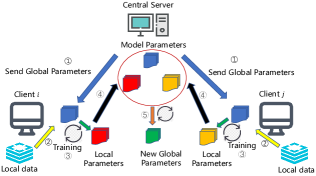
Figure 1: The schematic diagram of federal learning

As shown in Fig. 1, FL is a distributed ML paradigm in which a large number of mobile clients coordinate with the central server to learn an ML model without sharing their own training data [4]. During each global iteration, each client uses local data to perform batch stochastic gradient descent (SGD) to update the local model parameters, and the central server aggregates the local model parameters of all clients to generate new global model parameters for the next global iteration.

Given $N$ clients participating in training, we assume that each participating client $i\in\{1,...,N\}$ uses its local dataset $\mathcal{D}_{i}$ with data size $D_{i}$. Denote the collection of data samples in $\mathcal{D}_{i}$ as $\{\boldsymbol{x_{i}^{j}},y_{i}^{j}\}_{j=1}^{D_{i}}$, where $\boldsymbol{x_{i}^{j}}\in\mathbb{R}^{d\times 1},y_{i}^{j}\in\mathbb{R}$ refer to the input sample vector and the labeled output value, respectively. The loss function $f_{i}^{j}(\boldsymbol{w})$ is used to measure the difference between real output ${y_{i}^{j}}$ and predicted output ${{\hat{y}}_{i}^{j}}$. Then the loss function $F_{i}(\boldsymbol{w})$ of client $i$ on the dataset $\mathcal{D}_{i}$ is defined as:

$$F_{i}(\boldsymbol{w})=\frac{1}{D_{i}}\sum_{j\in{\mathcal{D}}_{i}}f_{i}^{j}(\boldsymbol{w}).$$ (1)

Without loss of generality, we denote the total training round of FL as $T$ and use a general principle of SGD optimization [18] to update the model. At iteration $t+1\in\{1,2,...,T\}$, each client updates the local parameters based on their own dataset and their own learning rate based on the last global parameters $\boldsymbol{w(t)}$ sent by the central server:

$$\boldsymbol{w_{i}(t+1)}=\boldsymbol{w(t)}-\eta_{i}\nabla F_{i}(\boldsymbol{w(t)}),$$ (2)

where $\eta_{i}$ is the learning rate of client $i$ and $\nabla F_{i}(\boldsymbol{w(t)})$ is the gradient of client $i$ at iteration $t$. The server averages the parameters sent back by $N$ training clients to generate the new global parameters:

$$\boldsymbol{w(t+1)}=\Sigma_{i=1}^{N}\theta_{i}\boldsymbol{w_{i}(t+1)},$$ (3)

where $\theta_{i}=\frac{D_{i}}{\sum_{j=1}^{N}D_{j}}$ is the weight of client $i$. Then the central server sends the updated global parameters $\boldsymbol{w(t+1)}$ to all clients for the next round’s training.

In general, the objective of the FL model is to find the optimal global parameters $\boldsymbol{w}$ to minimize the global loss function $F(\boldsymbol{w})$:

$$\underset{\boldsymbol{w}}{min}~{}F(\boldsymbol{w})=\Sigma_{i=1}^{N}\theta_{i}F_{i}(\boldsymbol{w}).$$ (4)

II-B Problem Formulation for Our Adaptive FL Strategy

In the traditional FL algorithms, each local client will use a static learning rate to train the model. However, there are some problems with this update method. First of all, it cannot adapt to parameters update for different clients, which will lead to the local model deviation from the optimal global model when the data distribution and devices of the clients are heterogeneous [8]. Moreover, the static learning rate reduces the convergence speed of the model as compared with the dynamic learning rate [20].

To solve the above problems, the following dynamic learning rate is introduced to update the local model parameters at iteration $t+1$:

$$\boldsymbol{w_{i}(t+1)}=\boldsymbol{w(t)}-\eta_{i}(t)\nabla F_{i}(\boldsymbol{w(t)}),$$ (5)

where $\eta_{i}(t)\in\mathbb{R}^{+}$ is the learning rate of client $i$ at iteration $t$.

In addition, the smaller the difference between each client’s parameters, the faster the model converges [21]. That is to say, the model will tend to converge when the local parameters of each client are similar. Note that the entropy function can be used to measure the diversity between variables. To spread out differences between the local parameters and achieve fast convergence, the entropy term $\Sigma_{i=1}^{N}p_{i}(t)\log p_{i}(t)=1$ with

$$p_{i}(t)=\frac{\theta_{i}\boldsymbol{w_{i}(t)}^{T}\boldsymbol{w_{i}(t)}}{\Sigma_{j=1}^{N}\theta_{j}\boldsymbol{w_{j}(t)}^{T}\boldsymbol{w_{j}(t)}}\in[0,1]$$ (6)

is introduced in the objective function $U_{i}(T)$ of client $i\in\{1,...,N\}$ for adaptive learning rate design:

$$U_{i}(T)=\underset{\begin{subarray}{c}\eta_{i}(t)\\ t\in\{0,...,T\}\end{subarray}}{min}\Sigma_{t=0}^{T}(\beta\Sigma_{j=1}^{N}p_{j}(t)\log p_{j}(t)+(1-\beta)\eta_{i}^{2}(t)),$$ (7)

s.t. $\boldsymbol{w_{i}(t+1)}=\boldsymbol{w(t)}-\eta_{i}(t)\nabla F_{i}(\boldsymbol{w(t)})$,   (5)

where $\beta$ controls the degree of aggregation.

However, there are two difficulties to solve in the optimization problem with the objective function $U_{i}(T)$. Firstly, it is difficult to solve the optimal dynamic learning rate by considering the huge number of learning rate combinations over time. Moreover, the design of learning rate $\eta_{i}(t)$ of client $i$ is not only affected by its own local parameters $\theta_{i}\boldsymbol{w_{i}(t)}^{T}\boldsymbol{w_{i}(t)}$, but also affected by the local parameters of other clients via the term $\Sigma_{j=1}^{N}\theta_{j}\boldsymbol{w_{j}(t)}^{T}\boldsymbol{w_{j}(t)}$. This makes the multi-agent joint learning rate design more challenging. To solve the above problem, we first derive the decentralized dynamic learning rate $\eta_{i}(t)$ for each client $i$ via a new mean-field approach, then we prove the existence of the approximate mean-field terms via fixed point theorem and propose a new algorithm to finalize the learning rate design.

III Analysis of Adaptive Learning Rate

In this section, we will find the optimal adaptive learning rate $\eta_{i}(t)$ for each client $i$ via a mean-field scheme. We first solve the adaptive learning rate $\eta_{i}(t)$ by constructing the mean-field terms $\boldsymbol{\phi_{1}(t)}$ and $\phi_{2}(t)$ to estimate the global parameters $\boldsymbol{w(t)}$ and $\Sigma_{i}^{N}\theta_{i}\boldsymbol{w_{i}(t)}^{T}\boldsymbol{w_{i}(t)}$, respectively. Then we prove the existence of the mean-field terms $\boldsymbol{\phi_{1}(t)}$ and $\phi_{2}(t)$ based the Brouwer’s fixed point theorem. Finally, we propose an algorithm used to find the adaptive learning rate.

III-A Adaptive Learning Rate for Each Client

In order to solve the adaptive learning rate for each client, we will first introduce the mean-field term that estimates the global weight $\Sigma_{j=1}^{N}\theta_{j}\boldsymbol{w_{j}(t)}^{T}\boldsymbol{w_{j}(t)}$. Note that $\Sigma_{j=1}^{N}\theta_{j}\boldsymbol{w_{j}(t)}^{T}\boldsymbol{w_{j}(t)}$ is the integration of local updated parameters obtained by various clients after local training. The learning rate will affect the local updated parameter of the individual client, as well as the value of $\Sigma_{j=1}^{N}\theta_{j}\boldsymbol{w_{j}(t)}^{T}\boldsymbol{w_{j}(t)}$, which in turn affects the local parameter updating and adaptive learning rate design. But other clients’ local information may be unknown when designing the adaptive learning rate for each client, especially for a large number of clients. Thus, we introduce the mean-field terms $\boldsymbol{\phi_{1}(t)},\phi_{2}(t),t\in\{0,...,T\}$ to estimate the $\sum_{i=1}^{N}\theta_{i}\boldsymbol{w_{i}(t)}$ and $\sum_{i=1}^{N}\theta_{i}\boldsymbol{w_{i}(t)}^{T}\boldsymbol{w_{i}(t)}$ respectively over time, i.e., we want to find two functions $\boldsymbol{\phi_{1}(t)}$ and $\phi_{2}(t)$ such that

$$\boldsymbol{\phi_{1}(t)}=\sum_{i=1}^{N}\theta_{i}\boldsymbol{w_{i}(t)},$$ (8)

$$\phi_{2}(t)=\sum_{i=1}^{N}\theta_{i}\boldsymbol{w_{i}(t)}^{T}\boldsymbol{w_{i}(t)}.$$ (9)

Then entropy term can be evaluated by:

$$\bar{p_{i}}(t)=\frac{\theta_{i}\boldsymbol{w_{i}(t)}^{T}\boldsymbol{w_{i}(t)}}{\phi_{2}(t)}\in[0,1].$$ (10)

The objective of client $i\in\{1,...,N\}$ becomes:

$$J_{i}(T)=\underset{\begin{subarray}{c}\eta_{t}(t)\\ t\in\{0,...,T\}\end{subarray}}{min}\Sigma_{t=0}^{T}(\beta\Sigma_{j=1}^{N}\bar{p_{j}}(t)\log\bar{p_{j}}(t)+(1-\beta)\eta^{2}_{i}(t)),$$ (11)

$$\text{s.t.}~{}~{}~{}\boldsymbol{w_{i}(t+1)}=\boldsymbol{\phi_{1}(t)}-\eta_{i}(t)\nabla F_{i}(\boldsymbol{\phi_{1}(t)})$$ (12)

According to the above system, the adaptive learning rate of each client $i$ is only affected by the mean-field terms $\boldsymbol{\phi_{1}(t)},\phi_{2}(t)$ and its local information. By constructing the Hamiltonian equation, we can obtain $\eta_{i}(t)$ as shown in the following proposition.

Proposition III.1

Given the mean-field term $\boldsymbol{\phi_{1}(t)}$ in (8), $\phi_{2}(t)$ in (9), $t\in\{0,1,...,T\}$, the optimal adaptive learning rate of client $i\in\{1,...,N\}$ at iteration $t\in\{0,1,...,T-1\}$ satisfies the following equation:

$$\begin{split}\eta_{i}(t)&=\Big{(}\frac{\theta_{i}(\boldsymbol{\phi_{1}(t)}-\eta_{i}(t)\nabla F_{i}(\boldsymbol{\phi_{1}(t)}))^{T}}{\phi_{2}(t+1)}\times\frac{\beta\nabla F_{i}(\boldsymbol{\phi_{1}(t)})}{(1-\beta)}\Big{)}\\ &*\Bigg{(}1+\log\bigg{[}\theta_{i}(\boldsymbol{\phi_{1}(t)}-\eta_{i}(t)\nabla F_{i}(\boldsymbol{\phi_{1}(t)}))^{T}\\ &\times\frac{(\boldsymbol{\phi_{1}(t)}-\eta_{i}(t)\nabla F_{i}(\boldsymbol{\phi_{1}(t)}))}{\phi_{2}(t+1)}\bigg{]}\Bigg{)},\end{split}$$ (13)

with $\eta_{i}(T)=0$.

Proof: Based on the objective function (11) with the mean-field terms $\boldsymbol{\phi_{1}(t)}$ and $\phi_{2}(t)$, we can construct the following Hamilton equation:

$$H(t) =\beta\Sigma_{j=1}^{N}\bar{p_{j}}(t)\log\bar{p_{j}}(t)+(1-\beta)\eta^{2}_{i}(t)$$ (14)

$$+\boldsymbol{\lambda_{i}(t+1)}(\boldsymbol{\phi_{1}(t)}-\eta_{i}(t)\nabla F_{i}(\boldsymbol{\phi_{1}(t)})-\boldsymbol{w_{i}(t)}),$$

where $\boldsymbol{\lambda_{i}(t+1)}\in\mathbb{R}^{1\times d}$ is a vector whose size is $1\times d$. Since $\frac{\partial^{2}H(t)}{\partial\eta_{i}^{2}(t)}=2(1-\beta)>0$, the Hamiltonian function $H(t)$ is convex in $\eta_{i}(t)$. Therefore, in order to find the optimal dynamic learning rate that minimizes the objective function $J_{i}(T)$ in (14), it is necessary to satisfy:

$$\frac{\partial H(t)}{\partial\eta_{i}(t)}=0,$$ (15)

$$\boldsymbol{\lambda_{i}(t+1)}-\boldsymbol{\lambda_{i}(t)}=-\frac{\partial H(t)}{\partial\boldsymbol{w_{i}(t)}}.$$ (16)

Based on Eq (15), we can derive:

$$2(1-\beta)\eta_{i}(t)+\boldsymbol{\lambda_{i}(t+1)}(-\nabla F_{i}(\boldsymbol{\phi_{1}(t)}))=0,$$ (17)

$$\eta_{i}(t)=\frac{\boldsymbol{\lambda_{i}(t+1)}\nabla F_{i}(\boldsymbol{\phi_{1}(t)})}{2(1-\beta)}.\\$$ (18)

According to Eq (16), we can get:

$$\begin{split}\boldsymbol{\lambda_{i}(t+1)}-\boldsymbol{\lambda_{i}(t)}&=\boldsymbol{\lambda_{i}(t+1)}-\bigg{(}\beta\frac{2\theta_{i}\boldsymbol{w_{i}(t)}^{T}}{\phi_{2}(t)}\\ &*\Big{(}\log\big{[}\frac{\theta_{i}\boldsymbol{w_{i}(t)}^{T}\boldsymbol{w_{i}(t)}}{\phi_{2}(t)}\big{]}+1\Big{)}\bigg{)}.\end{split}$$ (19)

$$\boldsymbol{\lambda_{i}(t)}=\beta\frac{2\theta_{i}\boldsymbol{w_{i}(t)}^{T}}{\phi_{2}(t)}\Big{(}\log\big{[}\frac{\theta_{i}\boldsymbol{w_{i}(t)}^{T}\boldsymbol{w_{i}(t)}}{\phi_{2}(t)}\big{]}+1\Big{)}.$$ (20)

By inserting $\boldsymbol{\lambda_{i}(t)}$ in (20) into the expression of $\eta_{i}(t)$ in (18), the optimal adaptive learning rate of client $i$ can be derived as Eq (13).  

Algorithm 1 Iterative Computation of Fixed Point

0:    Initiate the fixed point threshold $\varepsilon_{1}=0.001$, $\varepsilon_{2}=0.001$, global model parameter $w_{i}(0),i\in\{1,...N\}$, mean-field estimators $\boldsymbol{\phi_{1}^{0}(t)}$, $\phi_{2}^{0}(t)$, $t\in\{1,...,T\}$, $k=0$.

0:    The fixed point of the mean-field item $\boldsymbol{\phi_{1}(t)}$ and $\phi_{2}(t)$, $t\in\{1,2,...,T\}$.

1:  do

2:  for $t=0$ to $T-1$ do

3:     for $i=1$ to $N$ do

4:        compute $\eta_{i}(t)$ based on $\boldsymbol{\phi_{1}^{k}(t)},\phi_{2}^{k}(t)$, $t\in\{1,...,T\}$ according to Eq (13)

5:        compute $\boldsymbol{w_{i}(t+1)}$ according to Eq (12)

6:     end for

7:     compute $\boldsymbol{\phi_{1}^{k+1}(t+1)}$ according to Eq (8)

8:     compute $\phi_{2}^{k+1}(t+1)$ according to Eq (9)

9:  end for

10:  $k=k+1$

11:  while $\boldsymbol{\phi_{1}^{k}(t)}$-$\boldsymbol{\phi_{1}^{k-1}(t)}$ $\geq$ $\varepsilon_{1}$ and $\phi_{2}^{k}(t)-\phi_{2}^{k-1}(t)\geq\varepsilon_{2}$

III-B Update of Mean-Field Estimator for Finalizing Learning Rate

In this section, we determine the mean-field terms $\boldsymbol{\phi_{1}(t)}$ and $\phi_{2}(t)$ according to the given optimal adaptive learning rate $\eta_{i}(t)$ in (13). Note that the estimator $\boldsymbol{\phi_{1}(t)}$ and $\phi_{2}(t)$ which are constructed to estimate $\boldsymbol{w(t)}$ and $\Sigma_{i=1}^{N}\theta_{i=1}\boldsymbol{w_{i}(t)}^{T}\boldsymbol{w_{i}(t)}$ are affected by the local updated parameters $\boldsymbol{w_{i}(t)}$ of all clients, which will in turn affect the local parameters. In the following proposition, we will determine the appropriate mean-field estimators $\boldsymbol{\phi_{1}(t)}$ and $\phi_{2}(t)$ via fixed point theorem.

Proposition III.2

The mean-field estimators $\boldsymbol{\phi_{1}(t)},t\in\{0,1,...,T-1\}$ in (8) and $\phi_{2}(t),t\in\{0,1,...,T-1\}$ in (9) exist, as returned by Algorithm 1.

Proof: For any client $i\in\{1,...,N\}$, substitute $\boldsymbol{\phi_{1}(t)}=\Sigma_{i=1}^{N}\theta_{i}\boldsymbol{w_{i}(t)},\phi_{2}(t)=\sum_{i=1}^{N}\theta_{i}\boldsymbol{w_{i}(t)}^{T}\boldsymbol{w_{i}(t)}$ and $\eta_{i}(t)$ in (13) into (12), we can see that the local parameters $\boldsymbol{w_{i}(t)}$ of client $i$ at iteration $t$ is a function of the model parameters $\{\boldsymbol{w_{i}(t)}|t\in\{0,1,...,T\},i\in\{1,...,N\}\}$ of all the zones over time. Define the following function as a mapping from $\{\boldsymbol{w_{i}(t)}|t\in\{0,1,...,T\},i\in\{1,...,N\}\}$ to the model parameter of client $i$ $\boldsymbol{w_{i}(t)}$ in (13) at iteration $t$:

$$\Gamma_{i,t}(\{\boldsymbol{w_{i}(t)}|t\in\{0,1,...,T\},i\in\{1,...,N\}\})=\boldsymbol{w_{i}(t)}.$$ (21)

In order to summarize any possible mapping $\Gamma_{i,t}(*)$ in (21), we can define the following vector function as a mapping from $\{\boldsymbol{w_{i}(t)}|t\in\{0,1,...,T\},i\in\{1,...,N\}\}$to the set of all the clients’ model parameters over time:

$$\begin{split}&\Gamma(\{\boldsymbol{w_{i}(t)}|t\in\{0,1,...,T\},i\in\{1,...,N\}\})\\ =&\Big{(}\Gamma_{1,0}(\{\boldsymbol{w_{i}(t)}|t\in\{0,1,...,T\},i\in\{1,...,N\}\}),...,\\ &\Gamma_{1,T}(\{\boldsymbol{w_{i}(t)}|t\in\{0,1,...,T\},i\in\{1,...,N\}\}),....,\\ &\Gamma_{N,0}(\{\boldsymbol{w_{i}(t)}|t\in\{0,1,...,T\},i\in\{1,...,N\}\}),....,\\ &\Gamma_{N,T}(\{\boldsymbol{w_{i}(t)}|t\in\{0,1,...,T\},i\in\{1,...,N\}\})\Big{)}.\end{split}$$ (22)

Thus, the fixed point to $\Gamma(\{\boldsymbol{w_{i}(t)}|t\in\{0,1,...,T\},i\in\{1,...,N\}\})$ in (22) should be reached to let $\boldsymbol{\phi_{1}(t)}$ and $\phi_{2}(t)$ replicate $\sum_{i=1}^{N}\theta_{i}\boldsymbol{w_{i}(t)}^{T}\boldsymbol{w_{i}(t)}$ and $\Sigma_{i=1}^{N}\theta_{i}\boldsymbol{w_{i}(t)}$, respectively.

Firstly, $\boldsymbol{w_{i}(0)}$ as an initial model parameters value must be bounded for any client $i$. Thus, $\boldsymbol{\phi_{1}(0)}=\Sigma_{i=1}^{N}\theta_{i}\boldsymbol{w_{i}(0)}$ is bounded. According to Eq (13), we can derive:

$$\eta_{i}(t)=A_{i}(\boldsymbol{\phi_{1}(t)},\phi_{2}(t+1)),$$ (23)

where $A_{i}(*)$ is the analytic function of $\eta_{i}(t)$. Thus, we can obtain:

$$\begin{split}\phi_{2}(t+1)&=\Sigma_{i=1}^{N}\Bigg{(}\theta_{i}*\\ &\Big{(}\boldsymbol{\phi_{1}(t)}-A_{i}(\boldsymbol{\phi_{1}(t)},\phi_{2}(t+1))\nabla F_{i}(\boldsymbol{\phi_{1}(t)})\Big{)}^{T}\times\\ &\Big{(}\boldsymbol{\phi_{1}(t)}-A_{i}(\boldsymbol{\phi_{1}(t)},\phi_{2}(t+1))\nabla F_{i}(\boldsymbol{\phi_{1}(t)})\Big{)}\Bigg{)}.\end{split}$$ (24)

Then based on Eq (24), we can get:

$$\phi_{2}(t+1)=B(\boldsymbol{\phi_{1}(t)}),$$ (25)

where $B(*)$ is the analytic function of $\phi_{2}(t)$. Now we can derive:

$$\eta_{i}(t)=A_{i}(\boldsymbol{\phi_{1}(t)},B(\boldsymbol{\phi_{1}(t)})).$$ (26)

Based on Eq (26) and $A_{i}(*),B(*)$ are the analytic function, we can assume that the most at the maximum upper bound $C$ of $\eta_{i}(t)$:

$$0<\eta_{i}(t)\leq C.$$ (27)

Then we define the following local gradient bounded:

$$\|\nabla F_{i}(w_{i}(t))\|\leq D.$$ (28)

By inserting Eq (27), (28) into (12), we can get:

$$\begin{split}&\boldsymbol{w_{i}(1)}=\boldsymbol{\phi_{1}(0)}-\eta_{i}(0)\nabla F_{i}(\boldsymbol{\phi_{1}(0)}),\\ \end{split}$$ (29)

$$\boldsymbol{\phi_{1}(0)}-CD\leq\boldsymbol{w_{i}(1)}\leq\boldsymbol{\phi_{1}(0)}+CD,\\$$ (30)

$$\boldsymbol{\phi_{1}(0)}-CD\leq\boldsymbol{\phi_{1}(1)}\leq\boldsymbol{\phi_{1}(0)}+CD,$$ (31)

$$\boldsymbol{\phi_{1}(0)}-tCD\leq\boldsymbol{w_{i}(t)}\leq\boldsymbol{\phi_{1}(0)}+tCD.$$ (32)

Define set $\Omega=[\boldsymbol{\phi_{1}(0)}-CD,\boldsymbol{\phi_{1}(0)}+CD]\times...\times[\boldsymbol{\phi_{1}(0)}-TCD,\boldsymbol{\phi_{1}(0)}+TCD]$. Since $\Gamma_{i,t}$ is continuous, $\Gamma$ is a continuous mapping from $\Omega$ to $\Omega$. According to Brouwer’s fixed-point theorem, $\Gamma$ has a fixed point in $\Omega$.  

Algorithm 2 Federated Learning with Adaptive Learning Rate via Entropy (Adp_Entr)

0:    Initiate the global model parameter $\boldsymbol{w(0)}$, mean-filed terms $\phi_{1}(t),\phi_{2}(t),t\in\{0,1,..,T\}$ as returned by Algorithm 1, learning rate $\eta_{i}(-1)$, control parameter $\beta$, decay parameter $\gamma$ and the local training epoch of the client $E$.

0:    The optimal global model parameter $\boldsymbol{w(T)}$.

1:  for $t=0,...,T-1$ do

2:     $\boldsymbol{w_{i,0}(t)}=\boldsymbol{w(t)}$

3:     for each client $i\in\{1,2,...,N\}$ in parallel do

4:        Sample a random batch of data from $\mathcal{D}_{i}$ to compute the local gradient $\nabla F_{i}(w(t))$

5:        Solve $\eta_{i}(t)$ according to Eq (13), (33)

6:        for $k=0,...,E-1$ do

7:           Compute the local gradient $\nabla F_{i}(\boldsymbol{w_{i,k}(t)})$

8:           $\boldsymbol{w_{i,k+1}(t)}=\boldsymbol{w_{i,k}(t)}-\eta_{i}(t)\nabla F_{i}(\boldsymbol{w_{i,k}(t)})$

9:        end for

10:     end for

11:     $\boldsymbol{w(t+1)}=\Sigma_{i=1}^{N}\theta_{i}\boldsymbol{w_{i,E}(t+1)}$

12:  end for

As mentioned above, we summarize the process of solving fixed points in Algorithm 1. In addition, we use the following weight decay method to avoid excessive fluctuations in the learning rate:

$$\eta_{i}(t)=\gamma*\eta_{i}(t-1)+(1-\gamma)*\eta_{i}(t),$$ (33)

where $\gamma$ is the decay parameter. Refer to FedAvg [4], our adaptive federated learning process can be summarized in Algorithm 2 by considering $E$ local epochs performed by each client in parallel in every global iteration.

IV Experiments

In this section, we conduct simulation experiments on the MNIST dataset to evaluate the performance of our proposed adaptive learning FL algorithm. We first introduce how to set up the experiments. Then we compare the performance of our adaptive learning rate method with other FL algorithms in terms of model accuracy and convergence rate. Finally, we verify the impact of the penalty weight $\beta$ on the convergence performance of the FL model.

IV-A Experiment Setup

The experimental setup will be briefly introduced as follows.

Dataset: We use the MNIST dataset that is divided into training and test datasets. And there are 60,000 images in the test dataset and 10,000 images in the validation dataset. By default, the images in the MNIST dataset are 28x28 pixels, with a total of 10 categories.

Model: We use a linear model with a fully connected layer of input channel 784 and output channel 10.

Other FL Methods: The FL algorithms we mainly compare are FedAvg [4], FedAdam [11] and FedYogi [11].

Hyperparameters: Similar to [11], we set $\beta_{1}=0.9,\beta_{2}=0.99,\tau=10^{-5},\eta=10^{-2},\text{ and }\eta_{l}=10^{-2}$ for FedAdam and FedYogi. By default, let $\beta=0.99$, $\gamma=0.99$ and global iteration $T=50$. During each global iteration, the local client trains $E$ epochs with a batch size is 10. We consider $N=10$ clients and divide the Non-IID dataset similar to [8].

IV-B Comparison of the Algorithms

Methods	IID	Non-IID
FedAvg	0.925350010395050	0.868600070476532
FedAdam	0.926049888134002	0.875950068235397
FedYogi	0.926049917936325	0.860500067472457
Adp_Entr	0.924800097942352	0.896000087261200

TABLE I: The performance of different FL methods in MNIST dataset when the global iteration $T=50$ and local epoch $E=8$.

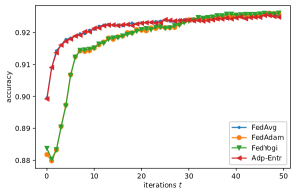
Figure 2: The performance of different FL methods on the IID data case when the global iteration $T=50$ and local epoch $E=8$.

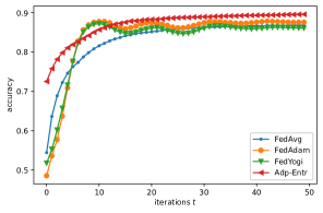
Figure 3: The performance of different FL methods on the Non-IID data case when the global iteration $T=50$ and local epoch $E=8$.

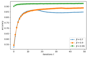
Figure 4: The impact of control parameter $\beta$ on the Non-IID data case.

We present the performance of different FL methods on the MNIST dataset as in Table I when the global iteration $T=50$ and local epoch $E=8$. For the IID dataset, there is not much difference between the several FL methods. As shown in Fig. 2, our method Adp_Entr converges faster than other adaptive models such as FedAdam and FedYogi. For the Non-IID client data distribution, our adaptive method achieves 2% accuracy improvement compared to other FL methods. Fig. 3 shows that our adaptive method converges faster and has higher accuracy than other methods. This indicates that our proposed adaptive method can effectively spread out the difference between different local parameters and achieve a faster convergent rate.

In addition, we analyze the influence of penalty parameter $\beta$ in Eq (7) on the model convergence performance. As shown in Fig. 4, with the increase of penalty weight $\beta$ on the diversity among the clients’ local parameters, our adaptive algorithm will try its best to minimize the difference between the local updating parameters, which leads to a faster convergent rate.

V Conclusion

In this paper, we discuss the convergent rate and accuracy of the global model in FL for Non-IID clients. Firstly, to achieve fast convergence, we utilize entropy theory to measure the difference between different local model parameters. Then, we propose the adaptive learning rate for each client via a mean-field approach, which effectively estimates the terms related to other clients’ model parameters over time and avoids frequent communication. Finally, the experimental results on the MNIST dataset show that the proposed adaptive learning rate algorithm has a higher accuracy and a faster convergent rate compared to other FL algorithms.

References

- [1] A. Ghosh, J. Chung, D. Yin, and K. Ramchandran, “An efficient framework for clustered federated learning,” Advances in Neural Information Processing Systems, vol. 33, pp. 19 586–19 597, 2020.
- [2] K. Bonawitz, V. Ivanov, B. Kreuter, A. Marcedone, H. B. McMahan, S. Patel, D. Ramage, A. Segal, and K. Seth, “Practical secure aggregation for privacy-preserving machine learning,” in proceedings of the 2017 ACM SIGSAC Conference on Computer and Communications Security, 2017, pp. 1175–1191.
- [3] Q. Yang, Y. Liu, T. Chen, and Y. Tong, “Federated machine learning: Concept and applications,” ACM Transactions on Intelligent Systems and Technology (TIST), vol. 10, no. 2, pp. 1–19, 2019.
- [4] B. McMahan, E. Moore, D. Ramage, S. Hampson, and B. A. y. Arcas, “Communication-Efficient Learning of Deep Networks from Decentralized Data,” in Proceedings of the 20th International Conference on Artificial Intelligence and Statistics, ser. Proceedings of Machine Learning Research, A. Singh and J. Zhu, Eds., vol. 54, 20–22 Apr 2017, pp. 1273–1282.
- [5] N. H. Tran, W. Bao, A. Zomaya, M. N. Nguyen, and C. S. Hong, “Federated learning over wireless networks: Optimization model design and analysis,” in IEEE INFOCOM 2019-IEEE conference on computer communications. IEEE, 2019, pp. 1387–1395.
- [6] A. Hard, K. Rao, R. Mathews, S. Ramaswamy, F. Beaufays, S. Augenstein, H. Eichner, C. Kiddon, and D. Ramage, “Federated learning for mobile keyboard prediction,” arXiv preprint arXiv:1811.03604, 2018.
- [7] Y. Zhao, M. Li, L. Lai, N. Suda, D. Civin, and V. Chandra, “Federated learning with non-iid data,” arXiv preprint arXiv:1806.00582, 2018.
- [8] T.-M. H. Hsu, H. Qi, and M. Brown, “Measuring the effects of non-identical data distribution for federated visual classification,” arXiv preprint arXiv:1909.06335, 2019.
- [9] S. P. Karimireddy, S. Kale, M. Mohri, S. Reddi, S. Stich, and A. T. Suresh, “Scaffold: Stochastic controlled averaging for federated learning,” in International Conference on Machine Learning. PMLR, 2020, pp. 5132–5143.
- [10] F. Sattler, S. Wiedemann, K.-R. Müller, and W. Samek, “Robust and communication-efficient federated learning from non-iid data,” IEEE transactions on neural networks and learning systems, vol. 31, no. 9, pp. 3400–3413, 2019.
- [11] S. J. Reddi, Z. Charles, M. Zaheer, Z. Garrett, K. Rush, J. Konečnỳ, S. Kumar, and H. B. McMahan, “Adaptive federated optimization,” in International Conference on Learning Representations, 2020.
- [12] A. Z. Tan, H. Yu, L. Cui, and Q. Yang, “Towards personalized federated learning,” IEEE Transactions on Neural Networks and Learning Systems, 2022.
- [13] T. Li, A. K. Sahu, M. Zaheer, M. Sanjabi, A. Talwalkar, and V. Smith, “Federated optimization in heterogeneous networks,” Proceedings of Machine Learning and Systems, vol. 2, pp. 429–450, 2020.
- [14] S. Wang, T. Tuor, T. Salonidis, K. K. Leung, C. Makaya, T. He, and K. Chan, “Adaptive federated learning in resource constrained edge computing systems,” IEEE Journal on Selected Areas in Communications, vol. 37, no. 6, pp. 1205–1221, 2019.
- [15] T. Nishio and R. Yonetani, “Client selection for federated learning with heterogeneous resources in mobile edge,” in ICC 2019-2019 IEEE international conference on communications (ICC). IEEE, 2019, pp. 1–7.
- [16] H. T. Nguyen, V. Sehwag, S. Hosseinalipour, C. G. Brinton, M. Chiang, and H. V. Poor, “Fast-convergent federated learning,” IEEE Journal on Selected Areas in Communications, vol. 39, no. 1, pp. 201–218, 2020.
- [17] Y. Chen, X. Sun, and Y. Jin, “Communication-efficient federated deep learning with layerwise asynchronous model update and temporally weighted aggregation,” IEEE transactions on neural networks and learning systems, vol. 31, no. 10, pp. 4229–4238, 2019.
- [18] H. Wu and P. Wang, “Fast-convergent federated learning with adaptive weighting,” IEEE Transactions on Cognitive Communications and Networking, 2020.
- [19] Q. Ma, Y. Xu, H. Xu, Z. Jiang, L. Huang, and H. Huang, “Fedsa: A semi-asynchronous federated learning mechanism in heterogeneous edge computing,” IEEE Journal on Selected Areas in Communications, vol. 39, no. 12, pp. 3654–3672, 2021.
- [20] S. Agrawal, S. Sarkar, M. Alazab, P. K. R. Maddikunta, T. R. Gadekallu, and Q.-V. Pham, “Genetic cfl: hyperparameter optimization in clustered federated learning,” Computational Intelligence and Neuroscience, vol. 2021, 2021.
- [21] F. Sattler, K.-R. Müller, and W. Samek, “Clustered federated learning: Model-agnostic distributed multitask optimization under privacy constraints,” IEEE transactions on neural networks and learning systems, vol. 32, no. 8, pp. 3710–3722, 2020.