On the functoriality of the space of equivariant smooth $h$-cobordisms

Abstract.

We construct an $(\infty,1)$-functor that takes each smooth $G$-manifold with corners $M$ to the space of equivariant smooth $h$-cobordisms $\mathcal{H}_{\textup{Diff}\,}(M)$. We also give a stable analogue $\mathcal{H}^{\mathcal{U}}_{\textup{Diff}\,}(M)$ where the manifolds are stabilized with respect to representation discs. The functor structure is subtle to construct, and relies on several new ideas. In the non-equivariant case $G=e$, our $(\infty,1)$-functor agrees with previous constructions of the smooth $h$-cobordism space as a functor to the homotopy category.

1. Introduction

The celebrated parametrized $h$-cobordism theorem, envisioned by Waldhausen and brought to fruition in seminal work of Waldhausen, Jahren, and Rognes, states that the stable space of piecewise-linear or topological $h$-cobordisms on a manifold $M$ is equivalent to the fiber of the $A$-theory assembly map,

and furthermore, the stable space of smooth $h$-cobordisms on a smooth manifold with boundary $M$ fits in a similar fiber sequence

[WJR13] gives a precise and detailed proof of the stable paramerized $h$-cobordism theorem in the PL case, which is then used to deduce the smooth version. Furthermore, if we assume that the stable $h$-cobordism spaces are functors, then these fiber sequences are natural in $M$.

The functoriality of $\mathcal{H}^{\infty}_{\textup{Top}}(M)$ and $\mathcal{H}^{\infty}_{\textup{PL}}(M)$ is easy to establish, but the functoriality of $\mathcal{H}^{\infty}_{\textup{Diff}\,}(M)$ is more subtle, and there does not seem to be a complete treatment in the literature. [Hat78, Wal82] provide sketches of how to define $\mathcal{H}^{\infty}_{\textup{Diff}\,}(M)$ as a functor to the homotopy category. Even defining the stabilization maps $\mathcal{H}_{\textup{Diff}\,}(M)\to\mathcal{H}_{\textup{Diff}\,}(M\times I)$ is a delicate problem, which is treated carefully in [Igu88].

To illustrate the problem, let us describe the standard method for making the unstable space of smooth $h$-cobordisms $\mathcal{H}_{\textup{Diff}\,}(M)$ into a functor on smooth manifolds and smooth embeddings. Given a smooth $h$-cobordism $W_{0}$ over $M_{0}$, and an embedding $M_{0}\to M_{1}$ with normal bundle $\nu$, we define a new $h$-cobordism $W_{1}$ on $M_{1}$ by taking the fiber product $W_{0}\times_{M_{0}}D(\nu)$, an $h$-cobordism over $D(\nu)$. It is not trivial on the sides, so we “pull up” a collar of the bottom to make it trivial. Equivalently, we bend the fiber product $W_{0}\times_{M_{0}}D(\nu)$ into a U-shape and glue in trivial regions above and below, as shown in Figure 1. (This idea was first introduced in [Igu88].)

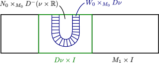
Figure 1. U-shaped stabilization of $W_{0}$ along $M_{0}\to M_{1}$.

This depends on choices, but the choices form a contractible space. So, we get a well-defined homotopy class of maps

$$\mathcal{H}_{\textup{Diff}\,}(M_{0})\to\mathcal{H}_{\textup{Diff}\,}(M_{1}).$$

For composable embeddings $M_{0}\to M_{1}\to M_{2}$, we need to show that these maps respect composition up to homotopy. If one ignores smooth structure, then this is not too difficult. Morally, the choice of smooth structure on the tricky bits is contractible, and so it should be possible to show that the rule respects composition up to homotopy. If we can prove this, then we stabilize by repeatedly embedding the manifolds $M$ into $M\times I$.

This may seem like a satisfactory sketch, but there is a significant issue. Even if all of the steps described above are accomplished and written down in detail, it only defines $\mathcal{H}^{\infty}_{\textup{Diff}\,}(M)$ as a functor to the homotopy category of spaces. To get the full strength of the naturality result in [WJR13, Thm 0.3], it is necessary to have a functor to the actual category of spaces, or at least an $(\infty,1)$-functor to the $(\infty,1)$-category of spaces. In other words, our functor does not have to respect the composition $M_{0}\to M_{1}\to M_{2}$ strictly, only up to a homotopy. If we then take a composite of three embeddings and the homotopies between all the two-fold compositions, those homotopies have to be coherent with each other. And so on.

This makes the problem easier, but even so, the sketch given above does not lead to a proof that $\mathcal{H}^{\infty}_{\textup{Diff}\,}(-)$ is an $(\infty,1)$-functor. It is not enough to know that the choices of data are contractible – one has to link the contractible choices together, showing that they are preserved under composition. And the most obvious ways of defining the contractible choices, e.g. choosing collars for $W_{0}$ and choosing the shape of the U-band, turn out to not be closed under composition, so they do not give an $(\infty,1)$-functor structure. We therefore have a nontrivial problem, that requires new ideas to solve.

Our main theorem is as follows. Since $(\infty,1)$-functors can be modeled by simplicially enriched functors, we state the result in terms of simplicially enriched functors. Let $G$ be a finite group, and let $\mathcal{H}_{\textup{Diff}\,}(M)$ denote the space of $G$-equivariant $h$-cobordisms over a compact $G$-manifold $M$. Let $\mathcal{M}^{\mathrm{Emb}}$ be the simplicial category of compact smooth $G$-manifolds and smooth equivariant embeddings.

Theorem 1.1.

There is a simplicially enriched functor

$$\mathcal{H}_{\textup{Diff}\,}(-)\colon\mathcal{M}^{\mathrm{Emb}}\to\textup{sSet}\,,$$

sending each compact $G$-manifold $M$ to a space equivalent to $\mathcal{H}_{\textup{Diff}\,}(M)$, and each homotopy class of equivariant embeddings $M_{0}\to M_{1}$ to the homotopy class of maps $\mathcal{H}_{\textup{Diff}\,}(M_{0})\to\mathcal{H}_{\textup{Diff}\,}(M_{1})$ given by the stabilization depicted in Figure 1.

Stabilizing the input $M$ by representation discs, we get a second functor $\mathcal{H}^{\mathcal{U}}_{\textup{Diff}\,}(M)$. We also prove that this stable $h$-cobordism space extends to all $G$-spaces:

Theorem 1.2.

The functor

$$\mathcal{H}^{\mathcal{U}}_{\textup{Diff}\,}(-)\colon\mathcal{M}^{\mathrm{Emb}}\to\textup{sSet}\,,$$

extends up to equivalence to a functor on the simplicial category of all $G$-CW complexes and equivariant continuous maps.

In the non-equivariant case $G=e$, Theorem 1.1 is closely related to the main result of the unpublished thesis [Pie18]. Pieper describes an $(\infty,1)$-functor structure on the smooth pseudoisotopy space, using an elaborate obstruction theory to show that one can simultaneously interpolate between different composites of U-bands. He obtains as a result the naturality of the $h$-cobordism splitting

$$A(X)\simeq Wh_{\textup{Diff}\,}(X)\times\Omega^{\infty}\Sigma^{\infty}_{+}X,\qquad\mathcal{P}^{\infty}_{\textup{Diff}\,}(X)\simeq\Omega^{2}Wh_{\textup{Diff}\,}(X).$$

It is a dense and technically impressive treatment, and unfortunately it appears that it will remain unpublished.

Our motivation for the current paper comes from current work of the first two authors on equivariant Reidemeister torsion, and separately of the last two authors on an equivariant stable parametrized $h$-cobordism theorem. Both of these projects require a functor structure on $\mathcal{H}_{\textup{Diff}\,}(M)$ in the equivariant case $G\neq e$. The prospect of expanding the treatment in [Pie18] to include equivariance seems daunting. Instead, we give a new approach that develops the $(\infty,1)$-functor structure in a simpler and more streamlined way.

We highlight three key ideas that make our approach work.

Instead of using U-shaped bands to stabilize cobordisms, we use polar stabilization, as pictured in Figure 2.

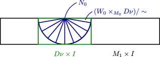
Figure 2. Polar stabilization of $W_{0}$ along $M_{0}\to M_{1}$.

This is an old idea, but there is a new feature. The innovation is to replace the space of cobordisms by an equivalent one in which each cobordism is equipped with an additional structure ensuring such that its polar stabilization is smooth and has the same kind of additional structure, so that it can be repeated multiple times without re-choosing collars. This makes it feasible to check coherence directly, instead of using a complicated and indirect obstruction theory as in [Pie18].

The extra structure is easy to describe: it is a choice of smooth structure on the double of $W_{0}$ along the top $N_{0}$ that extends the original smooth structure on each half. We call this a “mirror” structure. It exists and it is unique up to a contractible choice. The stabilization of a mirror $h$-cobordism is again canonically a mirror $h$-cobordism.

The second key idea is that in working with normal bundles of embeddings $M_{0}\to M_{1}$ we relax their structure, treating them as “round” disk bundles rather than the usual linear disk bundles. A round bundle is a smooth fiber bundle whose fiber is a disc, and whose structure group is the group of diffeomorphisms of the disc that preserve distance to the center – see Section 5.1. Round bundles have the advantage that they compose in a natural way along successive embeddings $M_{0}\to M_{1}\to M_{2}$, whereas vector bundles require additional contractible choices, and these choices are not easily made to be closed under composition.

The tradeoff for switching to round bundles is that it could be a priori more difficult to define the stabilization maps $\mathcal{H}_{\textup{Diff}\,}(M_{0})\to\mathcal{H}_{\textup{Diff}\,}(M_{1})$ using only the round structure on the normal bundle of $M_{0}\to M_{1}$. Miraculously, it turns out that it is not harder – it is actually a little easier. Pictorially, this means that it is more appropriate to think of the above polar stabilization using concentric circles, rather than rays, and to think of each circle as holding the points in $W_{0}$ that are at a single “height” along the cobordism.

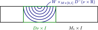
Figure 3. Polar stabilization defined using round bundles.

Lastly, we make use of the straightening-unstraightening theorem, originally due to Lurie [Lur09, 3.2.2]. It allows us to avoid defining the $(\infty,1)$-functor directly by specifying the spaces, maps, and coherent sets of homotopies. Rather, we define it indirectly by giving a fibration of $\infty$-categories with the correct lifting properties. The desired maps and homotopies then arise by universal properties.

To be more precise, we define the $h$-cobordism functor by specifying a map from a category object in simplicial sets to a simplicially enriched category,

(3) $$\mathcal{H}^{\mathrm{Stab}}\to\mathcal{M}^{\mathrm{Stab}}.$$

Taking nerves gives a map of Segal spaces, which we show is a left fibration. It follows from a version of the straightening-unstraightening theorem, specificially the version in [BdB18, Ras17], that this is equivalent to a simplicial functor from $\mathcal{M}^{\mathrm{Stab}}$ to spaces. Since $\mathcal{M}^{\mathrm{Stab}}$ is equivalent to the category of smooth manifolds and smooth embeddings, this gives the desired functor $\mathcal{H}_{\textup{Diff}\,}(-)$.

Theorem 1.1 and Theorem 1.2 give all of the functoriality one could hope for in the space of smooth $h$-cobordisms. In a subsequent paper, we use this functoriality to prove that the equivariant stable space of $h$-cobordisms splits into a product of non-equivariant stable $h$-cobordism spaces. The proof of this splitting takes a long detour through isovariant $h$-cobordism spaces, whose definition generalizes that of this paper, but with several additional subtleties. The construction of the stable equivariant $h$-cobordism space and the forthcoming splitting result are central to work in progress of the first two authors on equivariant Reidemeister torsion, and of the latter two authors on the equivariant stable parametrized $h$-cobordism theorem.

1.1. Outline

In Section 2, we establish and collect the necessary results about $G$-manifolds with corners. In Section 3, we describe the polar stabilization of pseudoisotopies. Even though our focus in this paper is on $h$-cobordisms, it is easiest to start with pseudoisotopies, because the technical lemmas we prove for pseudoisotopies are needed when stabilizing $h$-cobordisms.

In Section 4, we define the space of equivariant $h$-cobordisms on a smooth $G$-manifold with corners $M$. We also show that adding collars and mirror structure does not change the homotopy type of this space. In Section 5, we define the polar stabilization of smooth $h$-cobordisms. The construction of the smooth structure on this stabilization, and the proof that successive stabilizations give compatible smooth structures, form the technical core of the paper. As mentioned in the introduction, this requires choosing “mirror structure” on each cobordism, and the structure of a “round bundle” on the tubular neighborhoods.

In Section 6, we recall the notion of a left fibration of Segal spaces, following [BdB18, Ras17]. We then construct the map of simplicial categories (3) and take the associated left fibration, whose fibers are the $h$-cobordism spaces. Lastly, in Section 7, we stabilize the equivariant $h$-cobordism space with respect to all $G$-representations, and extend the resulting functor from smooth $G$-manifolds to all $G$-CW complexes.

1.2. Acknowledgments

We thank Wolfgang Lück for encouraging us to embark on this project of carefully working out the functoriality of the smooth $h$-cobordism space, and for making us aware of this gap in the literature. It is a pleasure to acknowledge contributions to this project arising from conversations with Mohammed Abouzaid, Julie Bergner, David Carchedi, Sander Kupers, Wolfgang Lück, Nima Rasekh, Emily Riehl, Hiro Lee Tanaka and Shmuel Weinberger. We especially thank David Carchedi and Nima Rasekh for directing us to the higher categorical results used in Section 6. We are very grateful to Dennis DeTurck, Herman Gluck, Ziqi Fang, Robert Kusner, and Leando Lichtenfelz for helping us think about Remark 5.5. We also thank Malte Pieper for sharing insights from his thesis with us.

Igusa was partially supported by Simons Foundation Grant 686616, Malkiewich was partially supported by NSF DMS-2005524 and DMS-2052923, and Merling was partially supported by NSF grants DMS-1943925 and DMS-2052988. This material is in part based on work supported by the National Science Foundation under DMS-1928930 while Merling was residence at the Simons Laufer Mathematical Sciences Institute (previously known as MSRI) in Berkeley, California, during the Fall 2022 semester. Lastly, Malkiewich and Merling thank the Max Planck Institute in Bonn, where they were in residence in the fall of 2018, and where the origins of this project can be traced back to.

2. Preliminaries on $G$-manifolds with corners

In this section we collect together the necessary technical results on $G$-manifolds with corners, where $G$ is a finite group. In particular, we require the existence of tubular neighborhoods for smooth embeddings, smooth approximations for continuous maps, the existence of collars, and smooth extensions of maps defined on the boundary $\partial M$ to an open neighborhood in $M$.

We claim no originality here – the results are either well-known or straightforward adaptions of existing arguments. We include them because the exact versions we need, in the presense of both corners and a $G$-action, can be difficult to find. We also highlight in Remark 2.15 a small surprise that occurs when one tries to smoothly extend a map from $\partial M$ to an open neighborhood in $M$.

2.1. $G$-manifolds with corners

Throughout, a manifold of dimension $n$ is always a smooth manifold with corners, i.e., a Hausdorff second-countable topological space $M$ with a maximal smooth atlas locally modeled on $[0,\infty)^{n}$, or equivalently on $[0,\infty)^{k}\times\mathbb{R}^{n-k}$ for $0\leq k\leq n$.

Definition 2.1.

A function on an open subset of $[0,\infty)^{k}\times\mathbb{R}^{n-k}$ is smooth if it extends to a smooth function on an open subset of $\mathbb{R}^{n}$. A map $f\colon M\to N$ between manifolds with corners is smooth if it is locally smooth in the sense that it corresponds via coordinate charts to a smooth map.

Definition 2.2.

The depth of a point $x$ in $M$ is the unique number $k$ such that there is a coordinate chart that identifies $x$ with the origin in an open subset of $[0,\infty)^{k}\times\mathbb{R}^{n-k}$. The set of all depth $0$ points is the interior of $M$. The set of depth $\geq 1$ points is the boundary subspace $\partial M\subset M$. Depth $\geq 2$ points are called corner points, and $\partial^{c}M\subset\partial M$ is the set of corner points.

Notice that $\partial M$ does not qualify as a smooth manifold with corners. (The corner points of $M$ lie in its interior.) It is of course a topological manifold.

Example 2.3.

A product of two or more manifolds with corners has the structure of a manifold with corners in a canonical way. For example, the $n$-dimensional cube $I^{n}$ and the polydisc $D^{n_{1}}\times\ldots\times D^{n_{k}}$ are manifolds with corners.

Example 2.4.

The standard $n$-simplex $\Delta^{n}$, with smooth structure inherited from $\mathbb{R}^{n+1}$, is a manifold with corners. The affine linear embedding $\Delta^{n}\to\mathbb{R}^{n}$ that takes one vertex to the origin and the remaining vertices to the standard basis vectors defines a diffeomorphism between the complement of one face in $\Delta^{n}$ and an open subset of $[0,\infty)^{n}$.

Because of Definition 2.1, the tangent space of a manifold with corners $M$ at a point $x\in M$ can be defined in the usual way using derivations of functions, even if the point is not in the interior. In the same way one defines the tangent bundle over all of $M$. Its total space is a smooth manifold with corners.

A diffeomorphism is a smooth map with smooth inverse, i.e. a homeomorphism that identifies the maximal atlases. The following is an easy consequence of the inverse function theorem.

Lemma 2.5.

A map $M\to N$ of smooth manifolds with corners is a diffeomorphism iff it is a smooth bijection and has invertible first derivative at every point of $M$ (including the boundary and corner points).

Smooth vector fields $\xi$ on a manifold with corners $M$ are defined in the obvious way, as smooth sections of the tangent bundle. In the presence of a group action we typically only consider $G$-invariant vector fields.

Following [Joy12], we define a manifold called the smooth boundary of $M$, whose interior may be identified with the set of depth $1$ points. This will be used later in discussing faces. For any point $x\in M$, one can define local boundary components near $x$ by intersecting a small enough neighborhood of $x$ with $\partial M\backslash\partial^{c}M$. Thus the depth of $x$ is the number of these. The smooth boundary $\widetilde{\partial}M$ is the set of pairs $(x,b)$ where $x\in M$ and $b$ is a local boundary component at $x$. This inherits a smooth atlas from $M$ so that $\widetilde{\partial}M$ becomes a smooth manifold with corners [Joy12, Definition 2.6.]. The map $i\colon\widetilde{\partial}M\to M$ that forgets the local boundary component is smooth, and its image is $\partial M$. It is not injective if $M$ has corner points.

Figure 4. The smooth boundary of a square consists of four line segments.

Definition 2.6.

Suppose that $M$ is a manifold with corners and that a finite group $G$ is acting smoothly on $M$. We say that the action is trivial on corners if any of the following equivalent conditions hold.

• For each boundary point $x\in\partial M$ with stabilizer $G_{x}$, the action of $G_{x}$ on the set of local boundary components near $x$ is trivial.

• $M$ is locally modeled by $G\times_{H}V\times[0,\infty)^{k}$, for varying $H\leq G$ and $H$-representations $V$.

• $M$ is locally modeled by finite products of smooth $G$-manifolds with boundary.

For example, a product $D(V_{1})\times\ldots\times D(V_{n})$, where each $D(V_{i})$ is the disk in a representation, has $G$-trivial action on corners, while the product $I\times I$ with action $(x,y)\mapsto(y,x)$ does not. We adopt the convention of only considering $G$-manifolds with $G$-trivial action on corners:

Definition 2.7.

A $G$-manifold with corners is a manifold with corners, with a smooth $G$ action that is trivial on corners.

Although the boundary subspace $\partial M$ is not a smooth manifold, it is locally modeled on $\partial([0,\infty)^{n})$ which is a subspace of $\mathbb{R}^{n}$, so we can still speak of smooth maps with domain $\partial M$. (A function on a subset $X$ of $\mathbb{R}^{n}$ is said to be smooth if near each point of $X$ it is the restriction of a smooth function from an open subset of $\mathbb{R}^{n}$.)

Lemma 2.8.

A map $f\colon\partial M\to N$ is smooth iff $f\circ i\colon\widetilde{\partial}M\to N$ is smooth.

Proof.

Since smoothness is defined locally, we may assume that $f$ is a map

$$\partial([0,\infty)^{k})\times\mathbb{R}^{n-k}\to\mathbb{R}^{m},$$

and we wish to extend $f$ smoothly to $[0,\infty)^{k}\times\mathbb{R}^{n-k}$. Let $V_{1},\ldots,V_{k}$ be the subspaces of the domain obtained by restricting one of the first $k$ coordinates to 0. Then $f$ is defined on the union of the $V_{i}$, and is smooth on each $V_{i}$ separately.

The question is unaffected if we subtract a function that admits a smooth extension to $[0,\infty)^{k}\times\mathbb{R}^{n-k}$. One such function is given by $f_{1}(x_{1},\dots,x_{n})=f(0,x_{2},\dots,x_{n})$. by projecting the first coordinate to 0 and then applying $f$. Replace $f$ by $f-f_{1}$. It now vanishes on $V_{1}$. Repeat with a second coordinate. Now the function vanishes on $V_{2}$ while still vanishing on $V_{1}$. Repeating with the remaining coordinates, $f$ now vanishes on every $V_{i}$, and therefore is zero. To put it another way, the original function $f$ is the sum of the functions $f_{i}$ that we have inductively defined. Each $f_{i}$ smoothly extends to $[0,\infty)^{k}\times\mathbb{R}^{n-k}$, so $f$ also extends in this way. ∎

Note that the lemma is also valid for equivariant maps of $G$-manifolds, since a local extension can always be made equivariant by averaging over the relevant isotropy subgroup of $G$.

2.2. Embeddings and tubular neighborhoods

A (smooth) embedding $M\to N$ is any smooth map that is a topological embedding and whose derivative has rank equal to the dimension of $M$ at every point, including corners. It is equivariant if it commutes with the action of $G$. It is a closed embedding or open embedding if it is topologically a closed or open embedding, respectively. It is elementary that $i$ is a closed embedding if it is smooth, full-rank, and injective, and if the source $M$ is compact.

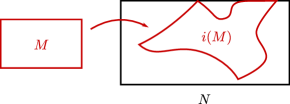
Figure 5. A smooth codimension 0 embedding of manifolds with corners.

Lemma 2.9.

If $i\colon M\to N$ is a smooth map of manifolds with corners (not necessarily compact) of the same dimension, and if $i$ is full-rank, injective, and depth-preserving, then it is an open embedding.

Proof.

We work locally at a point of depth $k$, so that without loss of generality $M$ and $N$ are neighborhoods of the origin in $[0,\infty)^{k}\times\mathbb{R}^{n-k}$ and $i$ preserves the origin. When $k=0$, openness is a standard consequence of the inverse function theorem. For higher values of $k$, inductively we know that the restriction of $i$ to each face of $[0,\infty)^{k}\times\mathbb{R}^{n-k}$ is open, so that the restriction to the boundary $\partial([0,\infty)^{k})\times\mathbb{R}^{n-k}$ contains a neighborhood of the origin. Therefore the image $i(\partial M)$ disconnects every sufficiently small neighborhood of the origin in $\mathbb{R}^{n}$.

Since $i$ has full rank, it admits an extension to an open neighborhood of the origin in $\mathbb{R}^{n}$ that is a homeomorphism to an open neighborhood in $\mathbb{R}^{n}$. By restricting the size of this neighborhood on the exterior of $[0,\infty)^{k}\times\mathbb{R}^{n-k}$, we can ensure that this extended version of $i$ does not send exterior points to interior points. Therefore the restriction to $[0,\infty)^{k}\times\mathbb{R}^{n-k}$ has image that is the intersection of an open set in $\mathbb{R}^{n}$ and the subspace $[0,\infty)^{k}\times\mathbb{R}^{n-k}$, which is exactly what we wanted. ∎

Lemma 2.10.

If $M$ is a compact $G$-manifold with corners, there is a closed embedding $M\to V$ into a sufficiently large orthogonal $G$-representation $V$.

Proof.

A standard proof of the non-equivariant statement can be adapted as follows. Cover $M$ by a finite set of coordinate charts that are preserved by the $G$-action, and take a partition of unity subordinate to this cover that is also $G$-invariant. This makes the resulting embedding (the coordinate charts scaled by the partition of unity) equivariant. ∎

The normal bundle of a smooth embedding is defined in the usual way, as the quotient of tangent bundles. Notice that this makes sense even at boundary and corner points. If the embedding is equivariant then the normal bundle is a $G$-vector bundle.

Definition 2.11.

For compact $G$-manifolds $M$ and $N$ and an equivariant embedding $i\colon M\to N$, a tubular neighborhood consists of a $G$-vector bundle $\nu\to M$ with invariant inner product and a codimension zero smooth equivariant embedding $\tilde{i}\colon D(\nu)\to N$ of the unit disk bundle extending $i$. Note that the embedding determines an isomorphism (of $G$-vector bundles without inner product) between $\nu$ and the normal bundle of $i$. Two tubular neighborhoods are considered equivalent if they are related by an isomorphism of $G$-vector bundles (preserving inner product). Thus in each equivalence class of tubular neighborhoods there is a representative in which $\nu$ is the normal bundle (with some inner product). There is a unique such representative such that the resulting isomorphism between $\nu$ and the normal bundle is the identity.

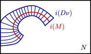
Figure 6. A tubular neighborhood of manifolds with corners.

We can also consider germs of tubular neighborhoods.

Definition 2.12.

A tubular neighborhood germ of the embedding $i:M\to N$ is given by a $G$-bundle $\nu\to M$, a $G$-invariant open subset $U\subseteq\nu$ containing the zero section, and a codimension zero embedding $\tilde{i}:U\to N$ extending $i$. Two such embeddings are said to give the same germ if they agree in some neighborhood of the zero section. Two germs are said to be equivalent if they related by a vector bundle isomorphism. Again there is a canonical representative for each class of germs, in which $\nu$ is the normal bundle of $i$.

Of course every tubular neighborhood determines a tubular neighborhood germ. Conversely, every tubular neighborhood germ is the germ of a tubular neighborhood. To see this, simply compose the given embedding $\tilde{i}:U\to N$ with an embedding $\nu\to U\subset\nu$, for example by using a diffeomorphism $[0,\infty)\to[0,\infty)$ that is the identity near zero and that sends $[0,1]$ into $[0,\epsilon)$ for some $\epsilon$. It will not always be necessary to distinguish carefully between tubular neighborhoods and their germs.

The usual proof of existence of tubular neighborhoods for embeddings into Euclidean space (e.g. [Hir94, Section 4.5]) applies in this equivariant setting:

Lemma 2.13.

If $M$ is a compact $G$-manifold with corners, every embedding into an orthogonal $G$-representation $V$ has a tubular neighborhood.

Proof.

For this argument we identify the normal space of $M$ at $x$ (a quotient of tangent spaces) with the space of vectors in $V$ that are perpendicular to the tangent space of $M$ at $x$. Now define $\tilde{i}$ by sending the vector $v\in V$ at the point $x\in M\subseteq V$ to $x+v\in V$. This map is clearly equivariant, and it is both full-rank and injective along $M$. It follows from a generalized version of the inverse function theorem that the map is full-rank and injective in a neighborhood of $M$, and from this it follows that it defines a tubular neighborhood germ. ∎

Note that a tubular neighborhood $D(\nu)$ for $M\to V$ comes with a smooth retraction $p$ from a neighborhood of $M$ in $D(\nu)$ to $M$, sending every point to its nearest neighbor in $M$. This retraction is useful for extending smooth maps from the boundary of a manifold with corners:

Lemma 2.14.

An equivariant map $f\colon\partial M\to\textup{int }N$ is smooth iff it extends to an equivariant smooth map $f\colon U\to N$ for an open subset $U\subseteq M$ containing $\partial M$.

Remark 2.15.

It is important that $f$ lands in the interior of $N$. If it hits boundary points then it is possible that no smooth extension exists. To give an example, let $M$ be $[0,\infty)^{3}$, let $N$ be $[0,\infty)$, and consider the quadratic form $x_{1}^{2}+x_{2}^{2}+x_{3}^{2}-c(x_{1}x_{2}+x_{1}x_{3}+x_{2}x_{3})$ with $1<c<2$. Since $c<2$, this maps $\tilde{\partial}M$ into $N$. On the other hand, any smooth real-valued function $f$ defined on a neighborhood of $\tilde{\partial}M$ in $M$ and agreeing with the quadratic form on $\tilde{\partial}M$ must agree with it to second order at the origin, and since $c>1$ this implies that $f(t,t,t)$ is negative for sufficiently small values of $t$.

Proof.

We give the proof in the special case that $M$ and $N$ are compact, but the general case is similar. Fix an equivariant smooth embedding $N\to V$ in a representation and choose an equivariant smooth retraction $p:\Omega\to N$ as above. The domain $\Omega$ is a neighborhood of $\textup{int }N$. Since $f(\partial M)$ is in the interior of $N$, $\Omega$ is a neighborhood of $f(\partial M)$ in $V$. It will be enough if $f$ has a smooth equivariant extension defined on a neighborhood of $\partial M$ and taking values in $\Omega$, for then we may compose $p$ with this extension. We construct the extension locally using Lemma 2.8 and then patch things together with a partition of unity.

In detail: Choose $\epsilon>0$ such that $\Omega$ contains every point of $V$ whose distance from $f(\partial M)$ is less than $\epsilon$. Choose also a continuous retraction $r$ from a neighborhood $U$ of $\partial M$ in $M$ to $\partial M$. Cover $\partial M$ by finitely many open sets $U_{i}\subset U$ such that $f$ has a smooth extension $f_{i}$ to $U_{i}$. Use a fine enough cover so that $f_{i}(x)$ is always in the $\epsilon$-ball with center $f(r(x))$. Now use a smooth partition of unity subordinate to this cover to add the resulting maps together as maps into $V$. Because all of the points $f_{i}(x)$ are within $\epsilon$ of $f(r(x))$, this stays inside $\Omega$. ∎

Lemma 2.13 gives the following corollary, see also [Was69, Corollary 1.12].

Corollary 2.16.

Any continuous equivariant map $f\colon M\to\textup{int }N$ can be approximated by a smooth equivariant map. If $f$ is smooth on a neighborhood of a closed subset $C\subseteq M$ then the smooth map can be taken to agree with $f$ on $C$.

Proof.

Take a non-equivariant smooth approximation rel $C$, and consider it as a map $M\to\textup{int }N\to V$. Conjugate by each element of $G$ and average the results together to produce another approximation $M\to V$ that is equivariant. Finally, apply a retraction $p$ as in the proof above to get the approximation $M\to\textup{int }N$. ∎

Recall from Definition 2.11 the definition of a tubular neighborhood.

Definition 2.17.

For an embedding $i:M\to N$ we define a space $\textup{Tub}_{\,\begin{picture}(-1.0,1.0)(0.5,-1.0)\circle*{1.8}\end{picture}\hskip 1.42271pt}(M)$ of tubular neighborhoods. A $k$-simplex assigns an equivariant tubular neighborhood to each point of $\Delta^{k}$ in such a way that the adjoint map $\Delta^{k}\times D(\nu)\to N$ is a smooth map of manifolds with corners. Since $D(\nu)$ is compact ([Gei18]), this is equivalent to asking that the track $\Delta^{k}\times D(\nu)\to\Delta^{k}\times N$ is a smooth embedding. (Compare to Definition 2.31 below.) Here $\nu$ is the normal bundle of $i$ (or any fixed bundle isomorphic to that), equipped with some invariant inner product.

Remark 2.18.

There is an analogous definition of a space of tubular neighborhood germs. The evident map from $\textup{Tub}_{\bullet}(M)$ to this is an equivalence; we omit the details.

Theorem 2.19 (Tubular Neighborhood Theorem, vector bundle version).

Assume $M$ is compact. For every equivariant embedding $i\colon M\to N$ landing in the interior of $N$, the space of equivariant tubular neighborhoods is a contractible Kan complex. Better, for any family of such embeddings $\Delta^{k}\times M\to N$, any system of tubular neighborhoods on $\partial\Delta^{k}$ can be extended to $\Delta^{k}$.

Proof.

Compactness of $M$ makes it easy to pass between germs and full neighborhoods, so we ignore the distinction here. We follow the usual proof as in [Hir94, Section 4.5], which goes in two stages. The first stage is Lemma 2.13, which shows the existence of one tubular neighborhood when $N=V$ is an orthogonal $G$-representation. Note that there is a continuous retraction $p$ of some open neighborhood of $M$ back to $M$ sending every point to the closest point in $M$, and that $p$ is smooth on the tubular neighborhood but only continuous on the rest of the open neighborhood of $M$.

To pass to the general case, we embed $N$ into an orthogonal $G$-representation $V$ and let $p$ be any smooth retraction to $N$ of any set that contains a neighborhood of the interior of $N$. Then we identify the normal bundle of $i$ as points in $M$ and vectors in $V$ that are tangent to the embedded $N$ and normal to $M$. Using this definition we then define $\tilde{i}$ by $\tilde{i}(x,v)=p(x+v)$. Since $i$ lands in the interior of $N$, so long as $v$ is sufficiently small this lands in the domain of $p$ and so the formula makes sense. We have therefore defined a tubular neighborhood germ.

To prove that the space of such neighborhood germs is contractible, we take any $\partial\Delta^{k}$ worth of such embeddings. Using Lemma 2.14, this extends to a $U_{0}$ worth of such embeddings where $U_{0}$ is a neighborhood of $\partial\Delta^{k}$ in $\Delta^{k}$. Then we take the “constant” tubular neighborhood described above on the interior of $\Delta^{k}$, and use a smooth partition of unity subordinate to $\{U_{0},\textup{int}\Delta^{k}\}$ to interpolate between these as maps into $\mathbb{R}^{n}$. Applying the retraction $p$ gives an interpolation as maps into $N$. Shrinking the domain of the germ if necessary, this is still a family of embeddings.

The argument works with the same formulas even if we allow the embedding $M\to N$ to change over $\Delta^{k}$, since the embedding $N\to\mathbb{R}^{n}$ is fixed throughout. ∎

A closed embedding is neat if it is locally modeled on the inclusion

$$[0,\infty)^{k}\times\mathbb{R}^{m-k}\times\{0\}^{n-m}\to[0,\infty)^{k}\times\mathbb{R}^{m-k}\times\mathbb{R}^{n-m}$$

with $m\leq n$, so in particular the depth of every point is preserved. Neat embeddings can have “neat” tubular neighborhoods, i.e. ones in which the map $\tilde{i}$ is an open embedding. Furthermore the space of neat tubular neighborhoods is contractible. However we will not need to prove such a statement in this paper.

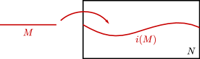
Figure 7. A codimension 1 neat embedding of manifolds with corners.

Definition 2.20.

A submersion of manifolds with corners is a smooth map locally modeled on the projection

$$[0,\infty)^{k}\times[0,\infty)^{k^{\prime}}\times\mathbb{R}^{\ell}\times\mathbb{R}^{\ell^{\prime}}\to[0,\infty)^{k}\times\{0\}\times\mathbb{R}^{\ell}\times\{0\}.$$

Note that when there are boundary points this condition is stronger than simply having full rank. For our submersions the derivative map of tangent spaces is surjective at each point, and additionally the derivative is surjective on the induced maps between different strata. By [Joy12, 5.1], these conditions are equivalent to being a submersion in our sense. The next result generalizes the Ehresmann fibration theorem to manifolds with corners.

Lemma 2.21.

Let $p\colon E\to M$ be an equivariant submersion of compact manifolds with corners. Then it is an equivariant smooth fiber bundle. Furthermore, if the base is $\Delta^{k}$ then the bundle is equivariantly diffeomorphic to a trivial bundle $\Delta^{k}\times F\to\Delta^{k}$.

Proof.

This follows from the usual proof of Ehresmann’s theorem. In more detail, let $\mathcal{V}$ be the class of vector fields $\xi$ on $E$ with the property that, in any chart on $E$ in which $p$ is a product as in Definition 2.20, the component of $\xi$ in the $[0,\infty)^{j}$ direction is, at each point, tangent to that point’s stratum in $[0,\infty)^{j}$. Note that $\mathcal{V}$ is convex and locally nonempty, and therefore globally nonempty using a partition of unity.

Near any point $x\in M$ locally modeled by $[0,\infty)^{k}\times\mathbb{R}^{\ell}$, we fix vector fields near $x$ that point in the coordinate directions. Using the product neighborhoods from Definition 2.20, we pick local lifts of each of these fields that lie in $\mathcal{V}$, and patch them together by a partition of unity to get a lift in $\mathcal{V}$ defined on an open subset containing $p^{-1}(x)$. Flowing along the resulting vector fields gives the desired local trivialization of $E$ near $x$. In the presence of a $G$-action, the proof is the same except that we also pick the fields to be $G$-invariant. ∎

2.3. Trimmings, faces, and collars

Let $M$ be a compact $G$-manifold with corners. A smooth ($G$-invariant) vector field on an open subset of $M$ containing $\partial M$ is inward pointing if for each point $x\in\partial M$, in one (therefore in all) charts the vector at $x$ points to the interior of $[0,\infty)^{k}\times\mathbb{R}^{n-k}$. Without loss of generality we may as well assume the vector field is defined on all of $M$. (It can be zero far away from $\partial M$.)

An embedded manifold with boundary $M^{\prime}\subseteq M$ is a trimming if there is a ($G$-invariant) inward-pointing vector field on $M$ that is nonvanishing on $M-\textup{int}\ M^{\prime}$, transverse to $\partial M^{\prime}$, and such that the integral curves give a homeomorphism $\partial M^{\prime}\cong\partial M$. In particular, this implies that $M^{\prime}\to M$ is continuously homotopic to a homeomorphism.

Figure 8. A trimming $M^{\prime}$ of a manifold with corners $M$.

Lemma 2.22.

Every compact $G$-manifold with corners has a trimming.

Proof.

Choose an inward-pointing vector field $\xi$, which exists by gluing together such fields locally using a smooth partition of unity on $M$. By averaging, we can assume that $\xi$ is $G$-invariant. As in [Wal82, Section 6], $\xi$ gives $\partial M$ a smooth structure in which the charts are obtained by taking discs transverse to $\xi$ and flowing to reach $\partial M$. We use this smooth structure on $\partial M$ throughout this proof.

Note that flowing along the vector field $\xi$ is defined for all positive times, since $M$ is compact and the field is inward-pointing. This gives us a map $\phi\colon\partial M\times[0,\infty)\to M$. Unfortunately, $\phi$ is not smooth, using the smooth structure on $\partial M$ described in the previous paragraph. However, it is still an open topological embedding.

Let $U=\phi(\partial M\times(0,1))$, with smooth structure coming from the fact that it is an open subset of $M$. Let $p\colon U\to\partial M$ be the projection back to $\partial M$. Although $\phi$ is not smooth, the projection $p$ is smooth, by construction. In fact, it is a smooth submersion whose fibers are open intervals. It therefore has a smooth section. This defines the boundary of the desired submanifold $M^{\prime}\subseteq M$. ∎

Proposition 2.23.

If $M$ is a compact smooth $G$-manifold with corners, there is an isotopy of equivariant embeddings from $\textup{id}_{M}$ to an embedding $M\to M$ sending $M$ into the interior.

Proof.

As before, choose an inward-pointing $G$-invariant vector field $\xi$. The flow along $\xi$ defines a smooth map $\phi\colon M\times[0,\infty)\to M$. Restricting to $M\times[0,1]$ gives the desired isotopy: at time $0$ it is the identity of $M$, and at time $1$, it is an embedding of $M$ into its interior. ∎

Corollary 2.24.

Every compact $G$-manifold with corners can be smoothly equivariantly embedded into the interior of another $G$-manifold with corners.

Combining Lemma 2.14 and Corollary 2.24, every map $\partial M\to N$ that is smooth as a map $\widetilde{\partial}M\to N$ extends to a smooth map $U\to N^{\prime}$, where $U$ is an open neighborhood of $\partial M$ in $M$, and $N^{\prime}$ is an open manifold containing $N$. By the counterexample in Remark 2.15, this is the best we can do in general.

Definition 2.25.

If $M$ is a $G$-manifold with corners, a face $F$ of $M$ is a $G$-invariant subspace of the smooth boundary $\widetilde{\partial}M$ such that

• $F$ is a union of components of $\widetilde{\partial}M$ and

• the map $i\colon\widetilde{\partial}M\to M$ is injective when restricted to $F$.

Example 2.26 (Faces).

We give some examples and nonexamples of faces.

1. Each side of the square $I\times I$ is a face, as is the union of two opposite sides. But the union of two adjacent faces is not, since the inclusion back to $I\times I$ is not injective.

2. The boundary of the $n$-simplex $\Delta^{n}$ consists of $n+1$ faces, each diffeomorphic to $\Delta^{n-1}$ as a manifold with corners.

3. In the teardrop-shaped 2-manifold, there are no faces. There is only one component in the smooth boundary, a closed interval whose endpoints both map under $i$ to the top of the teardrop, so $i$ is not injective on this component.

The following is an important consequence of Lemma 2.8, Lemma 2.14, and Corollary 2.24.

Corollary 2.27.

An equivariant map $M\times\partial\Delta^{n}\to N$ that is smooth on each face of $\Delta^{n}$ can always be smoothly, equivariantly extended to $M\times U\to N^{\prime}$, where $U$ is an open neighborhood of $\partial\Delta^{k}$ in $\Delta^{k}$, and $N^{\prime}$ contains $N$ in its interior.

Next we define collars on faces of a manifold with corners, which will play an important role in our definition of $h$-cobordisms.

Definition 2.28.

Let $F$ be a face of a $G$-manifold with corners $M$. A collar on $F$ is an extension of $F\to M$ to an equivariant embedding $c\colon F\times I\to M$ that preserves depth on $F\times[0,1)$ (and so is an open embedding on that subset). A collar is neat if it decreases depth by exactly 1 on $F\times\{1\}$.

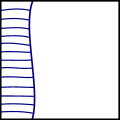
Figure 9. A neat collar for the left-hand face of a square.

Lemma 2.29.

Every face $F$ in a smooth compact $G$-manifold with corners $M$ has a neat collar $F\times I\to M$. Any two collars are isotopic through collars, and any two neat collars are related by an ambient isotopy of $M$.

As a result, we could re-define a face of $M$ to be a compact $G$-invariant subset $F\subseteq\partial M$ that has an open neighborhood diffeomorphic to $F\times[0,1)$.

Proof.

We can deform any collar to a neat collar by pre-composing with an isotopy of embeddings $I\to I$, so we focus on neat collars.

Note that near every point of $F$, the inclusion $F\to M$ is locally diffeomorphic to $F\to F\times I$. Consider $G$-invariant vector fields defined on all of $M$ with the following properties:

• for every point $x\in M\setminus F$ of depth $k$, the vector at $x$ lies in the tangent space of the stratum of depth $k$ points

• for every point $x\in F$ of depth $k$ in $F$ (so depth $k+1$ in $M$), when locally modeling $M$ as $F\times I$, the vector at $x$ lies in the tangent space of the manifold-with-boundary

  $$\textup{(depth $k$ points of $F$)}\times I,$$

  and is inward pointing (positive in the $I$ direction) at that point.

It is clear that the collection of fields with these conditions is convex. It is also nonempty because such fields exist locally, and we can add them together using a smooth partition of unity.

Each such vector field has unique integral curves defined starting from $F$, using for instance [Mel, Cor 1.13.1], and these curves are defined for all positive times $t\geq 0$ by our compactness assumptions. By the depth-preservation conditions, flowing along one such vector field until time $t=1$ provides a neat collar for the face $F$.

Conversely, any neat collar $F\times[0,1]\to M$ defines such a vector field on its image. We can then extend this vector field to the rest of $M$ using a smooth partition of unity and adding it to the zero vector field in all the other charts. So given two neat collars, we can linearly interpolate between these fields and get a one-parameter family of fields with the same condition. Flowing along these fields from $F$ defines a one-parameter family of neat collars.

To extend this to an ambient isotopy, we take the corresponding time-dependent vector field $F\times[0,1]\times[0,1]\to TM$ defined on the image of the isotopy, as in [Hir94, §8.1]. We extend this field to a time-dependent vector field $M\times[0,1]\to TM$ that is zero far away from this image, again using a smooth partition of unity. Flowing along this time-dependent field gives the desired ambient isotopy ([Hir94, 8.1.2]). ∎

Two collars are said to have the same germ if they agree on some $G$-invariant open neighborhood of the bottom and sides

$$(F\times\{0\})\cup(\partial F\times I)$$

inside $F\times I$. Just as with tubular neighborhoods, every collar germ is the germ of a collar:

Lemma 2.30.

If $M$ is compact, $F\subseteq M$ is a face, $L$ is an open subset of $F\times I$ containing the bottom and sides

$$(F\times\{0\})\cup(\partial F\times I)\subseteq L\subseteq F\times I,$$

and $\tilde{c}\colon L\to M$ is a partially-defined collar, then there is a collar $c\colon F\times I\to M$ whose germ agrees with that of $\tilde{c}$.

Proof.

By compactness there is an $\epsilon>0$ such that $L$ contains $F\times[0,\epsilon]$. Pick a smooth embedding $I\to I$ sending $I$ into $[0,\epsilon]$ and that is the identity near 0. Composing $\tilde{c}$ with this embedding gives an embedding $F\times I\to M$ that agrees with $\tilde{c}$ on a neighborhood of the bottom, though not the sides.

Now pick two $G$-invariant nested open neighborhoods $U_{0}\subseteq U_{1}\subseteq F$ containing $\partial F$ such that $U_{1}\times I\subseteq L$, and let $V_{1}$ be the complement of the closure of $U_{0}$. Pick a $G$-invariant partition of unity subordinate to the cover $\{U_{1},V_{1}\}$ and use it to add together the embedding $I\to I$ constructed above (on $V_{1}$) and the identity of $I$ (on $U_{1}$). The resulting equivariant embedding $F\times I\to F\times I$ agrees with the previous embedding outside of $U_{1}$, and is the identity outside of $V_{1}$. Therefore it is entirely contained in $L$. By construction it is also the identity near the bottom and sides. Therefore, composing with $\tilde{c}$ gives an equivariant collar $F\times I\to M$ whose germ agrees with that of $c$. ∎

This result will be useful – we will use germs of collars more than collars themselves.

2.4. Smooth simplices of diffeomorphisms

Suppose $W$ is a compact $G$-manifold with corners, $F\subseteq\partial W$ is a face, and and $C\subseteq\partial W$ is the closure of the complement of $F$ in $\partial W$. In particular, $C$ contains the boundary of $F$, and all of the corner points of $W$.

A diffeomorphism of $(W,F)$ is a diffeomorphism of $W$ that is the identity on some neighborhood of $C$. Thus it restricts to give a diffeomorphism of $F$ (which is the identity on a neighborhood of $\partial F$).

The simplicial group of diffeomorphisms of $(W,F)$ is defined using families of diffeomorphisms parametrized by $\Delta^{k}$ that correspond to smooth maps from $\Delta^{k}\times W$ to $W$:

Definition 2.31.

Let $\mathcal{D}_{\,\begin{picture}(-1.0,1.0)(0.5,-1.0)\circle*{1.8}\end{picture}\hskip 1.42271pt}(W,F)$ be the simplicial set whose $k$-simplices are (equivariant) diffeomorphisms $\Delta^{k}\times W\cong\Delta^{k}\times W$ over $\Delta^{k}$, that are the identity on $\Delta^{k}\times U$ for some open set $U$ containing $C$.

Lemma 2.32.

$\mathcal{D}_{\,\begin{picture}(-1.0,1.0)(0.5,-1.0)\circle*{1.8}\end{picture}\hskip 1.42271pt}(W,F)$ is a Kan complex, equivalent to the space of equivariant diffeomorphisms of $(W,F)$ with the $C^{\infty}$ topology.

Proof.

This proof is an adaptation of [Lur, Prop 1]. Let $\textup{Diff}\,(W,F)$ be the space of equivariant diffeomorphisms of $(W,F)$ with the $C^{\infty}$ topology. It suffices to take a diagram

and show that the bottom map can be changed by a simplicial homotopy rel $\partial\Delta[n]$ to a map for which a dotted lift exists. Indeed, we can then verify the Kan complex condition for $\mathcal{D}_{\,\begin{picture}(-1.0,1.0)(0.5,-1.0)\circle*{1.8}\end{picture}\hskip 1.42271pt}(W,F)$ by applying this fact twice, once to fill in the last face of the horn and again to fill in the interior. This condition demonstrates that the map is an isomorphism on simplicial homotopy groups, hence a weak equivalence because both simplicial sets are Kan complexes.

By Lemma 2.8, the top map corresponds to a smooth map $f\colon\partial\Delta^{n}\times W\to W$ and the bottom map is a continuous extension to

$$f\colon\Delta^{n}\times W\to W,$$

that at each point $t\in\Delta^{n}$ gives a diffeomorphism $f_{t}\colon W\to W$, that on some neighborhood $U_{t}$ of $C$ is the identity of $W$. (The partial derivatives in the $W$ direction are also continuous along the product $\Delta^{n}\times W$.) Furthermore, the neighborhoods $U_{t}$ can be chosen uniformly on each of the faces in $\partial\Delta^{n}$, and therefore over the entire boundary $\partial\Delta^{n}$. Call this uniform neighborhood $U_{0}$.

To deform this continuous family of diffeomorphisms to a smooth family, note that by Corollary 2.27, the restriction of $f$ to $\partial\Delta^{n}\times W$ extends to a smooth map $V_{0}\times W\to W^{\prime}$ for some open set $V_{0}\subseteq\Delta^{k}$ and some open extension $W^{\prime}$ of $W$. This will give smooth embeddings sufficiently close to $\partial\Delta^{n}$, but it will not necessarily give diffeomorphisms because the maps can fail to be surjective or to remain inside $W$. In addition, the embeddings may not be the identity on $U_{0}$.

To correct this, first extend to $V_{0}\times U_{0}$ by composing with the projection $V_{0}\times U_{0}\to U_{0}\subseteq W$. Then extend smoothly to the nontrivial face $V_{0}\times F\to F$. Note that the map is already given on an open neighborhood of the boundary of $F$, and therefore will stay inside $F$ provided $V_{0}$ is sufficiently small. Finally, extend these maps to $V_{0}\times W\to W^{\prime}$. Shrinking $V_{0}$ if necessary, each of the resulting maps $W\to W^{\prime}$ will be an embedding that is the identity on the neighborhood $U_{0}$ and sends the face $F$ to itself, therefore must send $W$ into itself, and therefore defines a diffeomorphism of $W$. Call this extension

$$f_{0}\colon V_{0}\times W\to W.$$

Next, pick a neat embedding of manifolds with boundary

$$W\setminus C\to\mathbb{R}^{n}\times[0,\infty),$$

so that $F\setminus C$ goes to $\mathbb{R}^{n}\times\{0\}$. Let $\pi$ be a smooth retract of a neighborhood back to $W$ that sends the points in $\mathbb{R}^{n}\times\{0\}$ to $F$. For each finite open cover $\{V_{i}\}_{i=1}^{n}$ of $\Delta^{n}-V_{0}$ by sets contained in the interior of $\Delta^{n}$, extend the cover to $\Delta^{n}$ by including $V_{0}$, then pick a smooth partition of unity $\{\phi_{i}\colon\Delta^{n}\to[0,1]\}$ subordinate to the resulting cover. Pick any point $t_{i}\in V_{i}$ and let $f_{i}=f_{t_{i}}$ be the diffeomorphism given by $f$ at $t_{i}$. Let $U_{i}$ be the neighborhood of $C$ on which $f_{i}$ is the identity. Then we define a new map $f^{\prime}\colon\Delta^{n}\times W\to W$ by the formula

$$f^{\prime}(w,t)=\pi\left(\sum_{i=0}^{n}\phi_{i}(t)f_{i}(t)\right).$$

It is clearly smooth and agrees with $f$ on $\partial\Delta^{n}$ by construction. It also respects a neighborhood $U$ of $C$ over the entire simplex, namely the intersection $\bigcap_{i=0}^{n}U_{i}$. By the assumption on $\pi$, it also preserves the face $F$ for each $t\in\Delta^{k}$. So long as the cover is fine enough, we can bound the $C^{1}$-distance from each $f^{\prime}_{t}$ to $f_{t}$, making each $f^{\prime}_{t}$ into an embedding as well. Again, since it is an embedding that respects the neighborhood $U$ pointwise and the face $F$ as a subspace, it must be a diffeomorphism.

Applying $\pi$ to a straight-line homotopy gives a deformation of this smooth family back to the original continuous family of diffeomorphisms. Again, this is through diffeomorphisms since they are embeddings and respect both $U$ and $F$. This concludes the proof. ∎

This gives us the following extension of Lemma 2.21. Consider an equivariant submersion of compact manifolds with corners $p\colon E\to\Delta^{k}$, with a face $F\subseteq\partial E$ such that the restricted map $F\to\Delta^{k}$ is also a submersion. By Lemma 2.21, we know that such a family can be trivialized to $\Delta^{k}\times(W,N)$ for some fixed manifold $W$ and face $N\subseteq\partial W$.

Corollary 2.33.

Any trivialization of $(E,F)$ that is defined on a proper union of $(k-1)$-dimensional faces $\cup_{i}D_{i}\subsetneq\partial\Delta^{k}$ can be extended to all of $\Delta^{k}$.

Proof.

Without loss of generality $(E,F)=(W,N)\times\Delta^{k}$, and so the given trivialization is a family of diffeomorphisms of $(W,N)$ defined on $\cup_{i}D_{i}$. By Lemma 2.32, $\mathcal{D}_{\,\begin{picture}(-1.0,1.0)(0.5,-1.0)\circle*{1.8}\end{picture}\hskip 1.42271pt}(W,N)$ is a Kan complex, so this family of diffeomorphisms can be extended to $\Delta^{k}$, giving the desired trivialization. ∎

3. Pseudoisotopies on manifolds with corners

In this section we consider the space of smooth pseudoisotopies on a compact smooth $G$-manifold with corners. We define an equivalent subspace, the space of “mirror” pseudoisotopies, designed in such a way that the “polar” stabilization of a mirror pseudoisotopy is again a mirror pseudoisotopy. This prepares the way for a similar construction involving spaces of smooth $h$-cobordisms.

3.1. Pseudoisotopies and mirror pseudoisotopies

Recall that for $W$ a compact $G$-manifold with corners, and $F\subseteq\partial W$ a face, Definition 2.31 gives a space $\mathcal{D}_{\,\begin{picture}(-1.0,1.0)(0.5,-1.0)\circle*{1.8}\end{picture}\hskip 1.42271pt}(W,F)$ of equivariant diffeomorphisms of $W$ that are the identity near the closure of $\partial W\setminus F$. The case of interest for us is when

$$W=M\times[-1,0]\cong M\times I$$

with $M$ a compact $G$-manifold with corners, and $F=M\times\{0\}$ is the top face. We call this the space of (equivariant) pseudoisotopies on $M$:

$$\mathcal{P}_{\,\begin{picture}(-1.0,1.0)(0.5,-1.0)\circle*{1.8}\end{picture}\hskip 1.42271pt}(M)=\mathcal{D}_{\,\begin{picture}(-1.0,1.0)(0.5,-1.0)\circle*{1.8}\end{picture}\hskip 1.42271pt}(M\times[-1,0],M\times\{0\}).$$

Let $r\colon M\times[-1,1]\to M\times[-1,1]$ be the reflection map $r(x,t)=(x,-t)$. Given a pseudoisotopy $f\colon M\times[-1,0]\to M\times[-1,0]$, the double of $f$ is the map

$$\bar{f}\colon M\times[-1,1]\to M\times[-1,1]$$

that commutes with $r$ and agrees with $f$ on $M\times[-1,0]$. Note that if we write $\bar{f}=(\bar{f}_{0},\bar{f}_{1})$ with

$$\bar{f}_{0}\colon M\times[-1,1]\to M$$

$$\bar{f}_{1}\colon M\times[-1,1]\to[-1,1]$$

then the requirement that $\bar{f}$ commutes with $r$ means that $\bar{f}_{0}(x,-t)=\bar{f}_{0}(x,t)$ and $\bar{f}_{1}(x,-t)=-\bar{f}_{1}(x,t)$ for all $x,t\in M\times[-1,1]$.

We call $f$ a mirror pseudoisotopy if its double $\bar{f}$ is smooth. In Figure 10, the pseudoisotopy on the right is mirror, while the one on the left is not.

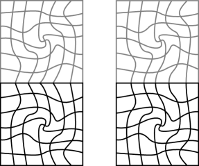
Figure 10. Two pseudoisotopies on $I$ and their doubles. The pseudoisotopy on the right is mirror, while the one on the left is not.

Let $\mathcal{P}_{\,\begin{picture}(-1.0,1.0)(0.5,-1.0)\circle*{1.8}\end{picture}\hskip 1.42271pt}^{\textup{mr}}(M)\subseteq\mathcal{P}_{\,\begin{picture}(-1.0,1.0)(0.5,-1.0)\circle*{1.8}\end{picture}\hskip 1.42271pt}(M)$ denote the subspace of those pseudoisotopies on $M$ that are mirror. Equivalently, these are the diffeomorphisms $\bar{f}$ of $M\times[-1,1]$ that are $(G\times C_{2})$-equivariant ($C_{2}$ being the group of order $2$, acting by $r$) and coincide with the identity on a neighborhood of the boundary. (Note that these conditions imply that the lower half of $M\times[-1,1]$ is sent to itself, so that $\bar{f}$ is in fact the double of some $f$.) When $f$ is mirror, we frequently drop the bar and just write $f$ for the double.

Lemma 3.1.

The inclusion $\mathcal{P}_{\,\begin{picture}(-1.0,1.0)(0.5,-1.0)\circle*{1.8}\end{picture}\hskip 1.42271pt}^{\textup{mr}}(M)\subseteq\mathcal{P}_{\,\begin{picture}(-1.0,1.0)(0.5,-1.0)\circle*{1.8}\end{picture}\hskip 1.42271pt}(M)$ is a weak equivalence.

Proof.

Call a pseudoisotopy regular if on some neighborhood $M\times(-\epsilon,0]$ of the top it coincides with the product of a diffeomorphism $M\to M$ and the identity in the $I$ coordinate. Note that regular implies mirror. For this proof, let $\mathcal{P}_{\,\begin{picture}(-1.0,1.0)(0.5,-1.0)\circle*{1.8}\end{picture}\hskip 1.42271pt}^{\rm reg}(M)$ consist of the ($\Delta^{k}$-families of) regular pseudoisotopies.

We will show that the inclusion $\mathcal{P}_{\,\begin{picture}(-1.0,1.0)(0.5,-1.0)\circle*{1.8}\end{picture}\hskip 1.42271pt}^{mr}(M)\subseteq\mathcal{P}_{\,\begin{picture}(-1.0,1.0)(0.5,-1.0)\circle*{1.8}\end{picture}\hskip 1.42271pt}(M)$ is a weak equivalence by showing that the same is true of the other inclusion and the composed inclusion in

$$\mathcal{P}_{\,\begin{picture}(-1.0,1.0)(0.5,-1.0)\circle*{1.8}\end{picture}\hskip 1.42271pt}^{reg}(M)\subseteq\mathcal{P}_{\,\begin{picture}(-1.0,1.0)(0.5,-1.0)\circle*{1.8}\end{picture}\hskip 1.42271pt}^{\textup{mr}}(M)\subseteq\mathcal{P}_{\,\begin{picture}(-1.0,1.0)(0.5,-1.0)\circle*{1.8}\end{picture}\hskip 1.42271pt}(M).$$

Given a $k$-simplex of pseudoisotopies $f$ (not necessarily mirror) that are regular along $\partial\Delta^{k}$, take the $k$-simplex of diffeomorphisms at the top

$$f_{0}\colon M\times\Delta^{k}\to M$$

and multiply by the identity of $[-1,0]$. We will deform $f$ through families of pseudoisotopies to one which agrees with $f_{0}\times 1$ near the top. Write $f=(f_{0}\times 1)\circ g$. We must deform $g$ to a diffeomorphism that coincides with the identity in a neighborhood of the top, and we need $g$ to be unchanged in a neighborhood of the bottom and sides and also over $\partial\Delta^{k}$. On $\partial\Delta^{k}$ the family of diffeomorphisms $g$ coincides with the identity near the top. Represent $g$ by vector fields flowing down from the top, then linearly interpolate the vector fields to point straight down (but fade out this modification so that far away from the top the vector fields do not change). Composing with $f_{0}\times\textup{id}$ gives a homotopy from $f$ to a family that is regular.

If the family $f$ is mirror then this entire procedure goes through mirror pseudoisotopies. This is because they are preserved by composition, and because a pseudoisotopy defined by a flow along a vector field $\xi=(\xi_{0},\xi_{1})$ transverse to $M\times\{0\}$ will be mirror iff the vector field satisfies $\xi_{0}(x,-t)=-\xi_{0}(x,t)$ and $\xi_{1}(x,-t)=\xi_{1}(x,t)$, and these conditions are preserved by linear interpolation. Since the procedure works for both ordinary and mirror pseudoisotopies, they are both equivalent to regular pseudoisotopies, giving the desired homotopy equivalence. ∎

3.2. Smoothness properties of even and odd functions

In order to understand the stabilization of a pseudoisotopy, we will need to recall some facts about even and odd functions. Let $M$ be any smooth manifold with corners. Let

$$r\colon M\times\mathbb{R}\to M\times\mathbb{R}$$

be the reflection map $r(x,t)=(x,-t)$. We say that a function

$$f\colon M\times\mathbb{R}\to\mathbb{R}$$

is odd if $f\circ r=-f$, and that a function

$$f\colon M\times\mathbb{R}\to X$$

to any set $X$ is even if $f\circ r=f$. These definitions also apply when $f$ is defined on an $r$-invariant subset of $M\times\mathbb{R}$, such as $M\times[-1,1]$.

Lemma 3.2.

If $f\colon M\times\mathbb{R}\to\mathbb{R}$ is smooth and odd then $f(x,t)=tg(x,t)$ for a smooth even function $g\colon M\times\mathbb{R}\to\mathbb{R}$.

Proof.

The following well known argument is valid even when $M$ has corners. Write $f_{2}(x,t)=\frac{\partial}{\partial t}f(x,t)$. Then

$$f(x,t)=\int_{0}^{t}f_{2}(x,u)du=t\int_{0}^{1}f_{2}(x,st)\ ds.$$

The last integral is a smooth function of $(x,t)$ by differentiation under the integral. ∎

Lemma 3.3.

If $f\colon M\times\mathbb{R}\to\mathbb{R}$ is smooth and even then $f(x,t)=g(x,t^{2})$ for a smooth function $g$.

Define $g(x,u)=f(x,\sqrt{u})$. In contrast to the previous lemma, this $g$ is only defined on $M\times[0,\infty)$, not all of $M\times\mathbb{R}$. We must prove that it is smooth.

Proof.

Recursively define a sequence of smooth even functions $h_{r}(x,t)$ on $M\times\mathbb{R}$, beginning with $h_{0}=f$. When $h_{r}$ has been defined, then because it is even its partial derivative with respect to $t$ is odd. By Lemma 3.2 we can factor out a $t$ (and a 2) and get a smooth even function $h_{r+1}$ such that

$$\frac{\partial h_{r}}{\partial t}(x,t)=2th_{r+1}(x,t).$$

We now prove by induction on $r$ that

$$\frac{\partial^{r}g}{\partial t^{r}}(x,t^{2})=h_{r}(x,t).$$

(and in particular that the left hand side is defined). Here the derivatives with respect to $t$ are defined in the usual way where $t>0$, and at $t=0$ they are defined as one-sided derivatives.

When $r=0$ this equality is true by the definition of $g$. Assuming the equality for a given $r$, we differentiate to get

$$2t\frac{\partial^{r+1}g}{\partial t^{r+1}}(x,t^{2})=\frac{\partial h_{r}}{\partial t}(x,t)=2th_{r+1}(x,t)$$

which gives the equality for $r+1$. This is valid for $t>0$; for $t=0$ we evaluate the $(r+1)$st derivative of $g$ to be

$$\frac{\partial}{\partial u}h_{r}(x,\sqrt{u})|_{u=0}=\lim_{u\to 0}\frac{h_{r}(x,\sqrt{u})-h_{r}(x,0)}{u}=\lim_{t\to 0}\frac{h_{r}(x,t)-h_{r}(x,0)}{t^{2}}$$

$$=\frac{1}{2}\frac{\partial^{2}}{\partial t^{2}}h_{r}(x,t)|_{t=0}=\frac{1}{2}\frac{\partial}{\partial t}(2th_{r+1}(x,t))|_{t=0}=h_{r+1}(x,0).$$

(Here the third to last equality used that $h_{r}$ is even.) This finishes the induction.

Finally, since $\frac{\partial^{r}g}{\partial t^{r}}(x,t)$ is equal to the continuous function $h_{r}(x,\sqrt{t})$, it has a $C^{0}$ extension to $M\times\mathbb{R}$. Integrating this $r$ times in the $t$ direction shows that $g$ admits a $C^{r}$ extension to $M\times\mathbb{R}$ for any $r\geq 0$. It now follows by [Mel, Theorem 1.4.1] or [Whi34] that $g$ is a smooth function. ∎

Corollary 3.4.

If $N$ is any smooth manifold with corners and $f\colon M\times\mathbb{R}\to N$ is smooth and even, then the function

$$g\colon M\times[0,\infty)\to N,\qquad g(x,t)=f(x,\sqrt{t})$$

is also smooth.

3.3. Stabilization

Recall that an (equivariant) pseudoisotopy $f$ is mirror if its double is smooth. Think of such a mirror pseudoisotopy as a diffeomorphism

$$f\colon M\times\mathbb{R}\to M\times\mathbb{R}$$

$$f(x,t)=(f_{0}(x,t),f_{1}(x,t))$$

such that $f_{0}$ is a $G$-equivariant even function to $M$, $f_{1}$ is a $G$-invariant odd function to $\mathbb{R}$, and $f$ is the identity on an open set containing $\partial M\times\mathbb{R}$ and all the points $(x,t)$ in which $|t|\geq 1$.

Given a mirror pseudoisotopy $f$ and an orthogonal $G$-representation $V$, define

$$\mathrm{St}^{V}f\colon M\times V\times\mathbb{R}\to M\times V\times\mathbb{R}$$

to be the function that applies $f$ along $M\times L$ for every line $L$ through the origin in $V\times\mathbb{R}$. In formulas,

$$(\mathrm{St}^{V}f)(x,v,t)=\left(f_{0}(x,\|(v,t)\|),\frac{v}{\|(v,t)\|}f_{1}(x,\|(v,t)\|),\frac{t}{\|(v,t)\|}f_{1}(x,\|(v,t)\|)\right).$$

The formula becomes simpler if we write $W=V\times\mathbb{R}$. Then for $(x,w)\in M\times W$ we have

$$(\mathrm{St}^{V}f)(x,w)=\left(f_{0}(x,\|w\|),\frac{w}{\|w\|}f_{1}(x,\|w\|)\right).$$

Note that when $\|w\|\geq 1$

$$(\mathrm{St}^{V}f)(x,w)=\left(x,\frac{w}{\|w\|}\cdot\|w\|\right)=(x,w).$$

As a result we can regard $\mathrm{St}^{V}f$ as a pseudoisotopy of $M\times D(V)$ instead of $M\times V$.

Lemma 3.5.

$\mathrm{St}^{V}f$ is smooth, $G$-equivariant, and mirror.

Proof.

It is straightforward to see that $f_{0}(x,\|(v,t)\|)$ and $\frac{v}{\|(v,t)\|}f_{1}(x,\|(v,t)\|)$ are even, $\frac{t}{\|(v,t)\|}f_{1}(x,\|(v,t)\|)$ is odd, and all three are $G$-equivariant. Clearly $\mathrm{St}^{V}f$ is smooth away from the cone point $w=0$. For smoothness at the cone point, note that by Lemma 3.2 and Corollary 3.4

$$(f_{0}(x,t),f_{1}(x,t))=(g_{0}(x,t^{2}),tg_{1}(x,t^{2}))$$

for some smooth equivariant functions $g_{0}$ and $g_{1}$ on $M\times[0,\infty)$, and therefore

$$(\mathrm{St}^{V}f)(x,w)=\left(g_{0}(x,\|w\|^{2}),w\cdot g_{1}(x,\|w\|^{2})\right).$$

The key is that $\|w\|^{2}$ is smooth (even though $\|w\|$ is not). Finally, $\mathrm{St}^{V}f$ is a diffeomorphism because its inverse is $\mathrm{St}^{V}(f^{-1})$. ∎

The same applies to a $k$-simplex of pseudoisotopies $\Delta^{k}\times M\times\mathbb{R}\to M\times\mathbb{R}$. The only difference is that now the functions $f_{0}$ and $f_{1}$ (and therefore $g_{0}$ and $g_{1}$ in the proof) depend smoothly on an extra argument $u\in\Delta^{k}$. The operation $\mathrm{St}^{V}$ clearly respects faces and degeneracies, and hence defines a map

$$\mathrm{St}^{V}\colon\mathcal{P}_{\,\begin{picture}(-1.0,1.0)(0.5,-1.0)\circle*{1.8}\end{picture}\hskip 1.42271pt}^{\textup{mr}}(M)\to\mathcal{P}_{\,\begin{picture}(-1.0,1.0)(0.5,-1.0)\circle*{1.8}\end{picture}\hskip 1.42271pt}^{\textup{mr}}(M\times D(V)).$$

The next lemma is functoriality for pseudoisotopies along inclusions of vector spaces.

Lemma 3.6.

For representations $V$ and $W$, $\mathrm{St}^{W\times V}f=\mathrm{St}^{W}\mathrm{St}^{V}f$.

Proof.

One can check this directly from the formulas, but it perhaps clearer to say this: $\mathrm{St}^{W}\mathrm{St}^{V}f$ applies $\mathrm{St}^{V}f$ along every subspace of $W\times V\times\mathbb{R}$ that is $V$ times a line in $W\times\mathbb{R}$, and $\mathrm{St}^{V}f$ applies $f$ along every line in this subspace, so that $\mathrm{St}^{W}\mathrm{St}^{V}f$ applies $f$ along every line in $W\times V\times R$, and this matches the definition of $\mathrm{St}^{W\times V}f$. ∎

As a result we get the commuting square

Remark 3.7.

For the most part, the results in this section serve as a technical underpinning and a plausibility check for the more sophisticated stabilization we perform later on $h$-cobordisms. It should be possible to go further and establish functoriality of pseudoisotopies along embeddings of manifolds, as in [Pie18], but we do not do so here.

4. $h$-cobordisms on manifolds with corners

In this section we define the space of $h$-cobordisms on a compact smooth $G$-manifold with corners. We also describe an extra structure that parallels the condition of a pseudoisotopy being mirror. This will help us form “polar” stabilizations of $h$-cobordisms just as for pseudoisotopies.

4.1. Definitions

Let $M$ be a compact smooth $n$-dimensional $G$-manifold with corners. An equivariant cobordism on $M$ is a compact $(n+1)$-manifold $W$ with corners, equipped with the following structure. There is a face of $W$ identified with $M$, called the bottom. There is a face $N$ of $W$, disjoint from $M$, called the top. The closure of the complement of $M\cup N$ in $\partial W$ is called the sides. There is an equivariant diffeomorphism between a neighborhood of the bottom and sides of $M\times[-1,0]$ and a neighborhood of the bottom and sides of $W$, taking $M\times\{-1\}$ to the bottom of $W$ and taking $\partial M\times[-1,0]$ to the sides of $W$, and therefore taking a neighborhood of $\partial M\times\{0\}$ in $M\times\{0\}$ to a neighborhood of $\partial N$ in $N$. We refer to this embedding of a neighborhood of $M\times\{-1\}\cup\partial M\times[-1,0]$ in $W$ as the lower collar and denote it by $c$.

(We use $[-1,0]$ instead of $[0,1]$ because later we will be doubling $W$ along the top and we like $[-1,1]$ better than $[0,2]$.).

Definition 4.1.

An equivariant $h$-cobordism on $M$ is a cobordism as above such that the inclusions $M\to W$ and $N\to W$ are equivariant homotopy equivalences.

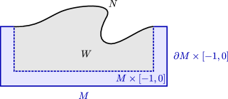
Figure 11. An $h$-cobordism on a manifold with corners $M$.

For definiteness, we fix a sufficiently large set $\mathcal{U}$ containing $M$ and assume that the underlying set of each cobordism $W$ is a subset of $\mathcal{U}$.

The double $\bar{W}$ of an $h$-cobordism $W$ is two copies of $W$ glued along their common top face $N$. We think of one as “flipped over” and use the interval $[0,1]$ in the place of $[-1,0]$, with $M$ located at 1 and $N$ located at 0.

Definition 4.2.

We define some structures on $h$-cobordisms.

1. A mirror $h$-cobordism is an $h$-cobordism $W$ together with a $(G\times C_{2})$-equivariant smooth structure on its double $\bar{W}$ that restricts to the smooth structure of $W$ on each copy of $W$ in the double.

2. Given a mirror $h$-cobordism, an encasing function is a smooth $G$-equivariant map

   $$\rho=(r,h)\colon W\to M\times[-1,0],$$

   having the following properties. The composition $\rho\circ c$ coincides with the identity map of $M\times[-1,0]$ in a neighborhood of the bottom and sides; in particular $r:W\to M$ is a retraction to the bottom. The function $h$ satisfies $h^{-1}(0)=N$, and the derivative $Dh$ has rank 1 along $N$; we call it the height function The map $\bar{W}\to M\times[-1,1]$, that extends $\rho$ and commutes with reflection is smooth. (We sometimes denote this extended map by $\rho$, or by $(r,h)$.) Note that the extended $\rho$ maps a neighborhood of the boundary of $\bar{W}$ to a neighborhood of the boundary of $M\times[-1,1]$ by a diffeomorphism.

An encased $h$-cobordism is a mirror $h$-cobordism equipped with an encasing function. This additional structure will be useful when we introduce stabilizations of $h$-cobordisms.

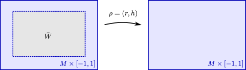
Figure 12. An encased $h$-cobordism.

Note that when making an encased $h$-cobordism it is redundant to specify the lower collar $c$, since it must coincide with the inverse of the encasing function $\rho$ near the boundary.

For a fixed mirror $h$-cobordism $W$, we can define a space of encasing functions by defining a $k$-simplex to be a smooth map $\Delta^{k}\times\bar{W}\to M\times[-1,1]$ that for each point of $\Delta^{k}$ defines an encasing function. We require there to be a single open neighborhood on which the encasing functions agree with $c^{-1}$, throughout the entire simplex $\Delta^{k}$.

Lemma 4.3.

The space of equivariant encasing functions on an equivariant mirror $h$-cobordism is contractible.

Proof.

The space of encasing functions is a product of two spaces, a space of retractions and a space of height functions, so we consider the two factors separately.

The set of height functions is nonempty and convex, and therefore contractible.

To see that it is nonempty, we create one height function on $\bar{W}$ by picking a bicollar for $N$ that agrees with the collar on $W$ near the sides (using Theorem 2.19), then using this bicollar to define the height function near $N$. We extend it continuously and equivariantly to the rest of $\bar{W}$ using that $[0,1]$ is contractible, then use smooth approximation (Corollary 2.16) to change the map rel the closure of a neighborhood of $N$ and the bottom and sides, to make it equivariant and smooth.

Then any other height function can be deformed by a straight-line homotopy to the given one. More generally any $k$-simplex of height functions may be deformed to the constant $k$-simplex in the same way. This yields a simplicial homotopy by triangulating $\Delta^{k}\times I$ in the usual prismatic way.

For retractions, suppose we have a $\partial\Delta^{k}$ worth of retractions. We use smooth extension (Lemma 2.14) to give us a $U$ worth of retractions where $U$ is an open neighborhood of $\partial\Delta^{k}$ inside $\Delta^{k}$. This is a map $U\times\bar{W}\to M$ that agrees with the projection to $M$ on a neighborhood $L$ of the bottom and sides of $\bar{W}$, so we get

$$(U\times\bar{W})\cup(\Delta^{k}\times L)\to M.$$

There is a slight problem in that some of the points in $U\times\bar{W}$ other than the sides $U\times(\partial M\times[-1,1])$ might be sent to $\partial M$, but this can be corrected by embedding $M$ in a larger open manifold and flowing along an inward-pointing vector field. Therefore outside of $\Delta^{k}\times L$, our map lands in the interior of $M$.

Since $M\to W$ is an equivariant homotopy equivalence, we can then extend this partially-defined retraction to a fully-defined retraction $\Delta^{k}\times\bar{W}\to M$, that is equivariant but only continuous. Since the region on which it is not smooth lands in the interior of $M$, we can again use equivariant smooth approximation (Corollary 2.16) to change the map to be smooth while leave it unchanged in a closed neighborhood of the boundary of $\Delta^{k}\times\bar{W}$. ∎

4.2. The space of $h$-cobordisms

Definition 4.4.

A diffeomorphism of $h$-cobordisms $W\cong W^{\prime}$ over $M$ is an (equivariant) diffeomorphism of manifolds with corners whose composition with the germ of the lower collar of $W$ is the germ of the given lower collar of $W^{\prime}$.

A mirror diffeomorphism between mirror $h$-cobordims is one whose extension to the doubles is also a diffeomorphism. An encased diffeomorphism is one that also commutes with the encasing functions.

Recall from Definition 2.31 that, for a compact manifold $W$ with face $F$, $\mathcal{D}_{\,\begin{picture}(-1.0,1.0)(0.5,-1.0)\circle*{1.8}\end{picture}\hskip 1.42271pt}(W,F)$ is the space (simplicial set) of equivariant diffeomorphisms that coincide with the identity in a neighborhood of $\overline{(\partial W\setminus F)}$. Therefore the space of diffeomorphisms of the $h$-cobordism $W$ is exactly $\mathcal{D}_{\,\begin{picture}(-1.0,1.0)(0.5,-1.0)\circle*{1.8}\end{picture}\hskip 1.42271pt}(W,N)$.

For a fixed manifold $M$, the desired homotopy type for the space of $h$-cobordisms $\mathcal{H}(M)$ is the disjoint union, over all diffeomorphism classes of $W$, of the classifying spaces $B\mathcal{D}_{\,\begin{picture}(-1.0,1.0)(0.5,-1.0)\circle*{1.8}\end{picture}\hskip 1.42271pt}(W,N)$. We could take this as our definition, but the following definition using families is more canonical and more convenient.

Definition 4.5.

A family of equivariant $h$-cobordisms over $\Delta^{k}$ is a smooth fiber bundle $p\colon E\to\Delta^{k}$ with $G$-action, whose fibers are equivariant $h$-cobordisms over $M$. Specifically it has a face $\Delta^{k}\times M\subseteq E$ and a lower collar $c\colon\Delta^{k}\times M\times[-1,0]\to E$, satisfying the same conditions on $c$ as in Definition 4.1. Again, it is only the germ of the collar along the bottom and sides that is considered to be part of the structure.

For definiteness we assume that each family has as its underlying set a subset of $\Delta^{k}\times\mathcal{U}$.

Families of mirror $h$-cobordisms are defined similarly, as are families of encased $h$-cobordisms. (In the latter case the retraction and height function that constitute the encasement are required to be smooth across the entire family.) We let $\bar{E}$ refer to the (fiberwise) double of the family $E$.

By Lemma 2.21, every $\Delta^{k}$-family of $h$-cobordisms can be trivialized, along with the lower collars. The same holds for mirror $h$-cobordisms, thinking of the double of the family $\bar{E}$ as a $(G\times C_{2})$-equivariant fiber bundle over $\Delta^{k}$ containing a trivial bundle (the germ of the bottom, sides, and their reflections).

Remark 4.6.

For a family of encased $h$-cobordisms, it is not true that the encasing function can be trivialized as well. In other words, we cannot assume the family is of the form $\Delta^{k}\times W$ with a single encasing function on $W$. If we imposed the assumption that the encasing functions were constant along families, it would make Proposition 4.12 below false.

Definition 4.7.

Let $M$ be a smooth compact $G$-manifold with corners. The space of equivariant $h$-cobordisms over $M$ is the simplicial set $\mathcal{H}_{\,\begin{picture}(-1.0,1.0)(0.5,-1.0)\circle*{1.8}\end{picture}\hskip 1.42271pt}(M)$ whose $k$ simplices are families of equivariant $h$-cobordisms over $\Delta^{k}$. Similarly, we define the space of mirror $h$-cobordisms $\mathcal{H}_{\,\begin{picture}(-1.0,1.0)(0.5,-1.0)\circle*{1.8}\end{picture}\hskip 1.42271pt}^{m}(M)$, and the space of encased mirror $h$-cobordisms $\mathcal{H}_{\,\begin{picture}(-1.0,1.0)(0.5,-1.0)\circle*{1.8}\end{picture}\hskip 1.42271pt}^{c}(M)$. The face and degeneracy maps are clear.

Lemma 4.8.

$\mathcal{H}_{\,\begin{picture}(-1.0,1.0)(0.5,-1.0)\circle*{1.8}\end{picture}\hskip 1.42271pt}(M)$ is a Kan complex.

Proof.

Given a horn $\Lambda^{k}_{i}\to\mathcal{H}_{\,\begin{picture}(-1.0,1.0)(0.5,-1.0)\circle*{1.8}\end{picture}\hskip 1.42271pt}(M)$, each face $\Delta^{k-1}\to\mathcal{H}_{\,\begin{picture}(-1.0,1.0)(0.5,-1.0)\circle*{1.8}\end{picture}\hskip 1.42271pt}(M)$ is a $\Delta^{k-1}$-family of $h$-cobordisms, which is isomorphic to a trivial family $W\times\Delta^{k-1}$. We identify the entire family with $W\times\Lambda^{k}_{i}$ by an induction on the faces, using Corollary 2.33.

Once the entire family has been identified with $W\times\Lambda^{k}_{i}$, we extend it to $W\times\Delta^{k}$. Then we take the underlying set of $W\times\Delta^{k}$ and apply a bijection to the subset $W\times\Lambda^{k}_{i}$ so that we get the underlying set of the original family (before trivialization). This produces a map $\Delta^{k}\to\mathcal{H}_{\,\begin{picture}(-1.0,1.0)(0.5,-1.0)\circle*{1.8}\end{picture}\hskip 1.42271pt}(M)$ that along $\Lambda^{k}_{i}$ strictly agrees with our original map. ∎

Lemma 4.9.

$\mathcal{H}_{\,\begin{picture}(-1.0,1.0)(0.5,-1.0)\circle*{1.8}\end{picture}\hskip 1.42271pt}(M)$ is equivalent to the disjoint union, over all diffeomorphism classes of $h$-cobordisms $W$ over $M$, of the classifying spaces $B\mathcal{D}_{\,\begin{picture}(-1.0,1.0)(0.5,-1.0)\circle*{1.8}\end{picture}\hskip 1.42271pt}(W,N)$.

Proof.

These spaces clearly have the same components, so we restrict to a single component $\mathcal{H}_{\,\begin{picture}(-1.0,1.0)(0.5,-1.0)\circle*{1.8}\end{picture}\hskip 1.42271pt}(M)_{[W]}$. Let $\mathcal{E}_{\,\begin{picture}(-1.0,1.0)(0.5,-1.0)\circle*{1.8}\end{picture}\hskip 1.42271pt}(M)_{[W]}$ denote the same simplicial set except that each family $E\to\Delta^{k}$ is equipped with a choice of trivialization $E\cong W\times\Delta^{k}$, and the face and degeneracy maps respect this trivialization.

Since every family in $\mathcal{E}_{\,\begin{picture}(-1.0,1.0)(0.5,-1.0)\circle*{1.8}\end{picture}\hskip 1.42271pt}(M)_{[W]}$ has a chosen trivialization, the entire simplicial set deformation retracts onto a single fixed 0-simplex. Specifically, we extend each $\Delta^{k}$ family $E\cong W\times\Delta^{k}$ to the $\Delta^{k+1}$ family given by $W\times\Delta^{k+1}$, but with the $\Delta^{k}$-face changed by a bijection on the underlying set so that it agrees with $E$.

Furthermore $\mathcal{E}_{\,\begin{picture}(-1.0,1.0)(0.5,-1.0)\circle*{1.8}\end{picture}\hskip 1.42271pt}(M)_{[W]}$ has a free action by the simplicial group $\mathcal{D}_{\,\begin{picture}(-1.0,1.0)(0.5,-1.0)\circle*{1.8}\end{picture}\hskip 1.42271pt}(W,N)$, changing the trivializations. The quotient by this action is $\mathcal{H}_{\,\begin{picture}(-1.0,1.0)(0.5,-1.0)\circle*{1.8}\end{picture}\hskip 1.42271pt}(M)_{[W]}$ (because by Lemma 2.21 every family can be trivialized). It follows that $\mathcal{H}_{\,\begin{picture}(-1.0,1.0)(0.5,-1.0)\circle*{1.8}\end{picture}\hskip 1.42271pt}(M)_{[W]}$ is a classifying space for $\mathcal{D}_{\,\begin{picture}(-1.0,1.0)(0.5,-1.0)\circle*{1.8}\end{picture}\hskip 1.42271pt}(W,N)$. ∎

Proposition 4.10.

The forgetful map from mirror to ordinary $h$-cobordisms

$$\mathcal{H}_{\,\begin{picture}(-1.0,1.0)(0.5,-1.0)\circle*{1.8}\end{picture}\hskip 1.42271pt}^{m}(M)\to\mathcal{H}_{\,\begin{picture}(-1.0,1.0)(0.5,-1.0)\circle*{1.8}\end{picture}\hskip 1.42271pt}(M)$$

is a weak equivalence of Kan complexes.

Proof.

The source is also a Kan complex by the same proof as in Lemma 4.8. We have a commuting diagram

(11)

where $\mathcal{H}_{G}^{v}(M)$ is the space of $h$-cobordisms equipped with the extra data of a germ of an inward pointing $G$-invariant vector field along the top face $N$ (as in the proof of Lemma 2.29). This is equivalent to giving the germ of a $G$-equivariant collar on $N$. Such a collar gives a mirror structure in a canonical way, by doubling it to a bicollar on $\bar{W}$ and using it to define the smooth structure at $N$.

It suffices to show that each diagonal map of (11) is a weak equivalence. This follows if we can produce lifts

            

For the first diagram, we first trivialize the family of cobordisms $E\cong W\times\Delta^{k}$, so that we can regard the vector fields as living on a fixed $h$-cobordism $W$. Then, as we observed in Lemma 2.29, the space of inward pointing vector fields on $W$ is convex and open. Given a family of such fields smoothly parametrized over $\partial\Delta^{k}$ we can extend it smoothly to an open neighborhood $U$ of $\partial\Delta^{k}$ in $\Delta^{k}$ by Lemma 2.14 (or Corollary 2.27), then cone it off to give a continuous extension to $\Delta^{k}$, then use smooth approximation (Corollary 2.16) to make the extension smooth on the interior of $\Delta^{k}$. Carrying the resulting family of fields from $W\times\Delta^{k}$ back to $E$ produces the desired lift.

For the second diagram the proof is the same except that we trivialize the family as a family of mirror $h$-cobordisms, and we restrict our attention to those inward pointing vector fields that respect the mirror structure on $W$. Specifically, we want the fields that are smooth when extended to $\bar{W}$ by applying the $C_{2}$ action and then negating the vectors. Note that if the mirror structure comes from a vector field then the vector field must have this property, so the given $\partial\Delta^{k}$ of vector fields has this property. Since the space of such fields is convex, we can extend as before to $\Delta^{k}$ and get the desired lift. ∎

Proposition 4.12.

The forgetful map from encased to mirror $h$-cobordisms

$$\mathcal{H}_{\,\begin{picture}(-1.0,1.0)(0.5,-1.0)\circle*{1.8}\end{picture}\hskip 1.42271pt}^{c}(M)\to\mathcal{H}_{\,\begin{picture}(-1.0,1.0)(0.5,-1.0)\circle*{1.8}\end{picture}\hskip 1.42271pt}^{m}(M)$$

is a weak equivalence of Kan complexes.

Proof.

It suffices to define lifts

Given a $\Delta^{k}$-family of mirror cobordisms with encasement data on $\partial\Delta^{k}$, we trivialize the family as before and then use Lemma 4.3 to extend the encasement over the rest of $\Delta^{k}$. ∎

Definition 4.13.

Suppose that $e\colon M\hookrightarrow M^{\prime}$ is a codimension 0 embedding. We define $W^{\prime}$, a mirror $h$-cobordism on $M^{\prime}$, by taking the double $\bar{W^{\prime}}$ to be the extension of $\bar{W}$ from $M$ to $M^{\prime}$ by the trivial cobordism. Here are the details. Topologically we take the pushout of

$$\overline{(M^{\prime}\setminus M)}\times[-1,1]\leftarrow\partial M\times[-1,1]\to\bar{W}.$$

To specify a smooth structure on this that restricts to the given smooth structures on $\overline{(M^{\prime}\setminus M)}\times[-1,1]$ and $\bar{W}$, we use the lower collar of $W$. The latter gives a definite way of identifying a neighborhood of $\partial M\times[-1,1]$ in $W$ with a neighborhood of $\partial M\times[-1,1]$ in $M\times[-1,1]$ and therefore a way of identifying a neighborhood of $\overline{(M^{\prime}\setminus M)}\times[-1,1]$ in $\bar{W^{\prime}}$ with a neighborhood of $\overline{(M^{\prime}\setminus M)}\times[-1,1]$ in $M^{\prime}\times[-1,1]$.

The encasing functions on $\bar{W}$ extend to $\bar{W^{\prime}}$ in the obvious way, and are smooth.

The same applies to families, so that a codimension zero embedding $M\to M^{\prime}$ yields a map $\mathcal{H}_{\,\begin{picture}(-1.0,1.0)(0.5,-1.0)\circle*{1.8}\end{picture}\hskip 1.42271pt}^{c}(M)\to\mathcal{H}_{\,\begin{picture}(-1.0,1.0)(0.5,-1.0)\circle*{1.8}\end{picture}\hskip 1.42271pt}^{c}(M^{\prime})$.

The following lemma establishes that the homotopy type of the $h$-cobordism space of a manifold with corners is not changed by rounding the corners. Recall the notion of trimming from Section 2.3.

Lemma 4.14.

If $M^{\prime}$ is a trimming of $M$ then the map $\mathcal{H}_{\,\begin{picture}(-1.0,1.0)(0.5,-1.0)\circle*{1.8}\end{picture}\hskip 1.42271pt}^{c}(M^{\prime})\to\mathcal{H}_{\,\begin{picture}(-1.0,1.0)(0.5,-1.0)\circle*{1.8}\end{picture}\hskip 1.42271pt}^{c}(M)$ induced by the embedding of $M^{\prime}$ in $M$ is a weak equivalence.

Proof.

In light of Proposition 4.10 and Proposition 4.12, it suffices to prove the same for the ordinary $h$-cobordism spaces $\mathcal{H}_{\,\begin{picture}(-1.0,1.0)(0.5,-1.0)\circle*{1.8}\end{picture}\hskip 1.42271pt}(M^{\prime})\to\mathcal{H}_{\,\begin{picture}(-1.0,1.0)(0.5,-1.0)\circle*{1.8}\end{picture}\hskip 1.42271pt}(M)$. We show that any diagram

(15)

admits a lift after modifying the horizontal maps by a homotopy of commuting squares. (A strict lift may not exist, because the map is not a Kan fibration.)

In geometric terms, this means we have a trivial family of $h$-cobordisms $W\times\Delta^{k}$ over $M$ such that for every point in $\partial\Delta^{k}$, the cobordism comes from a cobordism of $M^{\prime}$. This means that, as a cobordism over $M$, its lower collar has been extended to one whose domain contains $\overline{(M\setminus M^{\prime})}\times I$. (In the rest of $\Delta^{k}$ the lower collars lack this condition, instead only being open embeddings on $U_{0}\times I$ for some fixed open set $U_{0}$ containing $\partial M$.)

Pick an inward-pointing vector field in the sense of Section 2.3. By flowing along this field, we can produce a homotopy of diffeomorphisms of $M$, from the identity diffeomorphism, to one that sends $\overline{(M\setminus M^{\prime})}$ into $U_{0}$. Furthermore, throughout the homotopy, $\overline{(M\setminus M^{\prime})}$ is always sent into itself.

Take the lower collar germs for the entire family over $\Delta^{k}$ and pre-compose by this homotopy (times the identity of $I$). Those germs that were open embeddings on $\overline{(M\setminus M^{\prime})}$ continue to be so, and all of the remaining germs become open embeddings on $\overline{(M\setminus M^{\prime})}$ by the end. This produces the desired homotopy of the square (15) to one in which the lift exists. (We do not change the cobordisms, only their lower collars!) ∎

5. Stabilization of $h$-cobordisms

In this section we describe how a smooth embedding $M\to M^{\prime}$ determines a map of $h$-cobordism spaces $\mathcal{H}^{c}(M)\to\mathcal{H}^{c}(M^{\prime})$. In the case of a codimension zero embedding this was done in Definition 4.13. In the general case it is a two-step process: first use a cobordism over $M$ to make a cobordism over the total space of the normal disc bundle $D(\nu)$ of $M$ in $M^{\prime}$, and then extend along the codimension 0 embedding $D(\nu)\to M^{\prime}$ as before.

Although $\nu$ is a vector bundle, we will need to weaken its structure to something called a “round bundle” first. This is not necessary for defining the stabilization, but it becomes essential when we stabilize multiple times and compare the results. The structure of a vector bundle is too rigid – composites of vector bundles are not naturally vector bundles, and this creates an issue when composing tubular neighborhoods of successive embeddings.

5.1. Round diffeomorphisms

The composite of two disc bundles is not a disc bundle in a natural way. It is not just that the fiber is a product of discs instead of a disk; the structure group is also wrong.

Definition 5.1.

Let $V$ be an inner product space. A diffeomorphism $\rho\colon D(V)\to D(V)$ is round if $|\rho(v)|=|v|$ for all $v\in D(V)$. The round diffeomorphisms form a topological group $R(V)$ with the $C^{\infty}$ topology.

A round bundle is a smooth fiber bundle with fiber $D(V)$ and structure group $R(V)$. That is, it is a smooth fiber bundle with fibers diffeomorphic to $D(V)$ and with a preferred class of local smooth trivializations related by round diffeomorphisms. A $G$-equivariant round bundle is a round bundle with $G$-action (i.e. compatible smooth $G$-actions on base and total space) such that G acts through isomorphisms of round bundles, i.e., isomorphisms of bundles with structure group $R(V)$.

The inclusion $O(V)\subset R(V)$ is proper. For example, suppose that $V=V_{1}\oplus V_{2}$, $\phi\in O(V_{1})$, and we have a family of elements $\gamma_{v_{1}}\in O(V_{2})$ depending smoothly on $v_{1}\in V_{1}$. Then

$$(v_{1},v_{2})\mapsto(\phi(v_{1}),\gamma_{v_{1}}(v_{2}))$$

belongs to $R(V)$ but not in general to $O(V)$.

Lemma 5.2.

The inclusion $O(V)\to R(V)$ is a homotopy equivalence.

Proof.

For any $\rho\in R(V)$ the derivative $D_{0}\rho$ of $\rho$ at the origin belongs to $O(V)$. To see this, observe that

$$\frac{|\rho(v)-D_{0}\rho(v)|}{|v|}\to 0\quad\textup{ as }\quad v\to 0,$$

which implies that

$$\frac{|\rho(v)|}{|v|}-\frac{|D_{0}\rho(v)|}{|v|}\to 0\quad\textup{ as }\quad v\to 0.$$

Since $\frac{|\rho(v)|}{|v|}=1$ for all $v$, this means that $\frac{|D_{0}\rho(v)|}{|v|}\to 1$. But this last quantity is constant along rays, so it must be identically equal to $1$, and $|D_{0}\rho(v)|=|v|$ for all $v$. A linear map that preserves distance to the origin must belong to $O(V)$.

We can now make a deformation retraction from $R(V)$ to $O(V)$, using the homotopy

$$(\rho,t)\mapsto\frac{1}{t}\cdot\rho(t-).$$

At time $t=1$ this is equal to $\rho$. The limit as $t\to 0$ is $D_{0}\rho$. ∎

Corollary 5.3.

Every equivariant smooth round bundle is smoothly isomorphic (as an equivariant round bundle) to the unit disc bundle of an equivariant Euclidean vector bundle.

Proof.

We deduce this not from Lemma 5.2 but from its proof. (One issue is smooth versus topological isomorphism of bundles. The other is that when nontrivial $G$-action on the base of the bundle is allowed then equivariant bundles do not simply correspond to bundles with a certain structure group.)

We first prove the statement for trivial $G$. Given a round bundle $E_{1}\to M$, the homotopy of Lemma 5.2 defines a smooth bundle $E\to M\times I$, which at one endpoint is the original bundle $E_{1}\to M\times\{1\}$, and at the other end is a smooth round bundle $E_{0}\to M\times\{0\}$ whose structure group is $O(V)$, so that it arises from a vector bundle.

To be more specific, we present $E_{1}$ by preferred local trivializations $U\times D(V)$ and clutching functions $\phi(-)\colon U\cap U^{\prime}\to R(V)$. We then define $E$ by taking the spaces $U\times I\times D(V)$, and gluing them together along the clutching functions $(U\times I)\cap(U^{\prime}\times I)\to R(V)$ defined by $\frac{1}{t}\cdot\phi(t-)$. When $t=0$, these clutching functions land in $O(V)$, as desired.

We need to ensure that $E$ can be trivialized in the $I$-direction as a round bundle, so that $E_{0}\cong E_{1}$ as round bundles. We arrange that by choosing a lift to $E$ of the standard vector field in $M\times I$ pointing in the $I$-direction. The lift should be such that in any preferred local trivialization $U\times I\times D(V)$, the component of the vector field along $D(V)$ has no radial component. Note that this condition is preserved by the clutching functions, since the clutching functions take values in the round diffeomorphism group $R(V)$. We may therefore define such fields in each trivialization $U\times I\times D(V)$ separately, and patch them together by a partition of unity.

When flowing along such a vector field, each integral curve maintains a constant distance to the origin in $D(V)$. Thus the flow is through round diffeomorphisms. This proves that we can trivialize $E$ in the $I$-direction as a round bundle, so that $E_{0}\cong E_{1}$ as round bundles.

In the presence of a $G$-action preserving the round structure, this proof can be carried out equivariantly. We define the $G$-action on $E$ the same way we define the clutching functions, by taking the existing action of each element $g\in G$ on $E_{1}$ and extending it to $E$ by the map $\frac{1}{t}\cdot g(t-)$. When $t=0$, this is a linear action on each fiber, making $E_{0}$ into the disc bundle of an equivariant Euclidean vector bundle. The vector fields in $E$ with no radial component are preserved by this action, so we construct such a field non-equivariantly as before, then average it over $G$ to construct such a field that is $G$-invariant. Flowing along this $G$-invariant field, we get an isomorphism of equivariant round bundles $E_{0}\cong E_{1}$. ∎

Corollary 5.4.

For finite groups $G$, every homomorphism $G\to R(V)$ is conjugate to a homomorphism $G\to O(V)$.

Remark 5.5.

In the non-equivariant case, Corollary 5.3 would follow directly from Lemma 5.2 using the main result of [MW09], if we knew that the structure group of round diffeomorphisms forms a Frechet Lie group. This is known for $\textup{Diff}\,(D^{n})$, but seems more difficult to show for the subgroup of round diffeomorphisms. We leave this as an open question which may be interesting in its own right.

The point of round bundles is that they allow us to compose tubular neighborhoods of successive embeddings without selecting additional trivialization data. Given round bundles $E\to A$ and $A\to B$ with fibers $D(V_{2})$ and $D(V_{1})$ respectively, the composite bundle has fiber $D(V_{1})\times D(V_{2})$. We define the round composite of the bundles by starting with $E\to B$ and then restricting to the subset of $E$ whose fiber over $b\in B$ is the subset of $D(V_{1})\times D(V_{2})$ corresponding to $D(V_{1}\times V_{2})$. In other words we restrict attention to those points in $E$ such that $s^{2}+t^{2}\leq 1$ where $s$ is the norm in the fiber of $E\to A$ and $t$ is the norm of the image in the fiber of $A\to B$. The round composite is again a round bundle with fiber $D(V_{1}\times V_{2})$. What makes this well-defined independent of local trivialization is that a twisted product of round diffeomorphisms

always restricts to a round diffeomorphism of $D(V_{1}\times V_{2})$.

We need a variant of Theorem 2.19 for round bundles. A round tubular neighborhood of $M\to N$ is a smooth $G$-invariant codimension 0 submanifold $D\subseteq N$ containing $M$, a smooth equivariant map $p\colon D\to M$ that is a left inverse of the inclusion of $M$, and the structure of an equivariant round bundle on $p$. These are considered up to the appropriate equivalence relation. In view of Corollary 5.3, a round tubular neighborhood corresponds to an equivalence class of vector bundle tubular neighborhoods in the sense of Definition 2.17, where two such are identified if there is a round isomorphism of the disc bundles commuting with the embedding into $N$.

Theorem 5.6 (Tubular Neighborhood Theorem, round bundle version).

Assume $M$ is compact. For every family of equivariant embeddings $i\colon M\times\Delta^{k}\to N$ landing in the interior of $N$, any system of round tubular neighborhoods on $\partial\Delta^{k}$ can be extended to $\Delta^{k}$.

Proof.

By Corollary 5.3, the given system of round tubular neighborhoods refines to a system of vector tubular neighborhoods. By Theorem 2.19, the system of vector tubular neighborhoods can be extended over the interior. But that extension is, by neglect of structure, an extension as a system of round tubular neighborhoods. ∎

5.2. The stabilization and its smooth structure

Let $M$ be a compact $G$-manifold with corners, let $W$ be a mirror $h$-cobordism on $M$, and suppose that $W$ is equipped with an encasing function. We follow the notation of the previous section, letting $N$ be the top of the cobordism and denoting the double by $\bar{W}$.

We will make an encased $h$-cobordism $St^{\nu}(W)$ on the manifold $D(\nu)$, where $\nu$ is the normal bundle of an embedding $e:M\to M^{\prime}$ and $D(\nu)\to M$ is its closed unit disc bundle. We define $St^{\nu}(W)$ by defining its double $St^{\nu}(\bar{W})$.

For the next definition, $p\colon D(\nu)\to M$ may be any equivariant round bundle. Let $D(\nu\times\mathbb{R})\to M$ be the round composite of $p$ with the trivial bundle

$$D(\nu)\times[-1,1]=D(\nu)\times D(\mathbb{R})\to D(\nu).$$

In addition to the projection $D(\nu\times\mathbb{R})\to M$ this has a map to $[0,1]$, namely the norm in the fiber over $M$. On the other hand, $W$ also has a map to $M\times[0,1]$, namely the encasing function $\rho$ to $M\times[-1,0]$ flipped upside down. We can therefore form the fiber product

$$W\times_{M\times[0,1]}D(\nu\times\mathbb{R}).$$

This space will be the essential part of $St^{\nu}(\bar{W})$.

For an inner product bundle $\xi$, let $S(\xi)$ be the total space of the unit sphere bundle. Let $D_{0}(\xi)\subset D(\xi)$ be the zero section, homeomorphic to the base of the bundle. Let $D_{0}^{\prime}(\xi)$ be the complement of $D_{0}(\xi)$ in $D(\xi)$.

Consider the map

$$W\times_{M}S(\nu\times\mathbb{R})\to W\times_{M\times[0,1]}D(\nu\times\mathbb{R})$$

given by $(w,u)\mapsto(w,|h(w)|u)$. This maps the open subset $(W\backslash N)\times_{M}S(\nu\times\mathbb{R})$ homeomorphically to the open subset $(W\backslash N)\times_{M\times(0,1]}D_{0}^{\prime}(\nu\times\mathbb{R})$. It maps the complementary closed subset $N\times_{M}S(\nu\times\mathbb{R})$ onto the closed set $N\times_{M\times\{0\}}D_{0}(\nu\times\mathbb{R})$, and when we identify this last set with $N$ the map becomes the projection $(n,u)\mapsto n$.

The fiber product $W\times_{M\times[0,1]}D(\nu\times\mathbb{R})$ can therefore be rewritten as the colimit

Let $C(\nu\times\mathbb{R})$ denote the complement of the interior of $D(\nu\times\mathbb{R})$ inside $D(\nu)\times[-1,1]$, so that $D(\nu)\times[-1,1]$ is the union of $C(\nu\times\mathbb{R})$ and $D(\nu\times\mathbb{R})$ along $S(\nu\times\mathbb{R})$.

Definition 5.7.

As a topological space with $G$-action, $\mathrm{St}^{\nu}(\bar{W})$ is the colimit of the diagram

or more simply the colimit of

The middle horizontal map is induced by the inclusion of $M\cong M\times\{-1\}$ into $W$.

The group $C_{2}$ acts on $\mathrm{St}^{\nu}(\bar{W})$ by flipping the $\mathbb{R}$ direction. The set of $C_{2}$-fixed points is the fiber product

$$W\times_{M\times[0,1]}D(\nu),$$

which in Figure 13 corresponds to the center line. The whole is the double of the lower half along its top, and this lower half is called $\mathrm{St}^{\nu}(W)$.

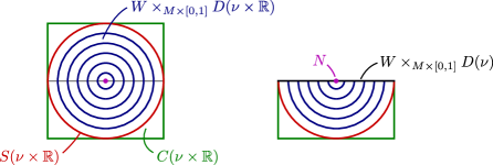
Figure 13. The doubled stabilization $\mathrm{St}^{\nu}(\bar{W})$ and its lower half $\mathrm{St}^{\nu}(W)$.

Before providing a smooth structure, we verify that we have made a topological equivariant $h$-cobordism.

Lemma 5.8.

If $W$ is $G$-equivariantly homotopy equivalent to its top and bottom, then so is $\mathrm{St}^{\nu}(W)$.

Proof.

Pick a presentation of $\nu$ as a vector bundle, not just a round bundle. Then deformation retract $C(\nu\times\mathbb{R})$ in the $\mathbb{R}$-direction back to $S(\nu\times\mathbb{R})$, then shrink the rest to the center using the $G$-equivariant deformation retraction of $W$ to $N$. Throughout the homotopy we vary the corresponding point in $D(\nu\times\mathbb{R})$ by scaling in the radial direction (for which we need the vector bundle structure). This shows that the inclusion of $N$ into $\mathrm{St}^{\nu}(W)$ is a $G$-equivariant homotopy equivalence.

The same homotopy shows that $N$ is also equivalent to the top of $\mathrm{St}^{\nu}(W)$. Therefore $\mathrm{St}^{\nu}(W)$ is equivariantly homotopy equivalent to its top. The zig-zag of subspaces of $\mathrm{St}^{\nu}(W)$

and equivariant homotopy equivalences now shows that the inclusion of the bottom $D(\nu)$ into $\mathrm{St}^{\nu}(W)$ is an equivalence as well. ∎

The following language will help us talk about $\mathrm{St}^{\nu}(\bar{W})$ more efficiently.

• The trivial region of $\mathrm{St}^{\nu}(\bar{W})$, pictured in green in Figure 13, is $C(\nu\times\mathbb{R})$.

• The nontrivial region of $\mathrm{St}^{\nu}(\bar{W})$, pictured in blue in Figure 13, is

  $$W\times_{M\times[0,1]}D(\nu\times\mathbb{R}).$$

• The frontier of $\mathrm{St}^{\nu}(\bar{W})$, pictured in red in Figure 13, is the intersection

  $$S(\nu\times\mathbb{R})=N\times_{M\times\{1\}}S(\nu\times\mathbb{R})$$

  of the trivial and nontrivial regions.

• The cone locus of $\mathrm{St}^{\nu}(\bar{W})$, pictured in purple in Figure 13, is the set

  $$N\times_{M\times\{0\}}D_{0}(\nu\times\mathbb{R})\cong N$$

  inside the nontrivial region.

Definition 5.9.

We define the smooth structure on the double $\mathrm{St}^{\nu}(\bar{W})$ as follows.

The interior of the trivial region $C(\nu\times\mathbb{R})$ has an obvious smooth structure. Moreover, the map $D(\nu\times\mathbb{R})\to M\times[0,1]$ is a submersion over the interior of $[0,1]$, giving the fiber product $W\times_{M\times[0,1]}D(\nu\times\mathbb{R})$ an induced smooth structure away from 0 and 1. We still need to define the smooth structure near the frontier and near the cone locus.

To define a smooth structure near the frontier $S(\nu\times\mathbb{R})$, we use the lower collar of $W$ to identify a neighborhood of the frontier in the nontrivial region with a neighborhood of $S(\nu\times\mathbb{R})$ in $D(\nu\times\mathbb{R})$, and thus to identify a neighborhood of the trivial region in $St^{\nu}(\bar{W})$ with a neighborhood of $C(\nu\times\mathbb{R})$ in the smooth manifold $D(\nu)\times[-1,1]$

It remains to define a smooth structure at the cone locus $N$. For each $n\in N$, pick a contractible neighborhood $U\to N$ of $n$ and a collar

$$b:U\times(-\epsilon,0]\to W,$$

such that the double

$$b:U\times(-\epsilon,\epsilon)\to\bar{W}$$

is smooth. Choose it such that $h\circ b$ is projection on the second factor; this is possible because the height function has full rank. It should also be equivariant with respect to the isotropy group $G_{n}\subset G$.

Choose also a smooth trivialization of the round bundle $D(\nu)\to M$ near $r(n)\in M$, compatible with the action of $G_{r(w)}$. Pulling this back to $\bar{W}$ and adding on $\mathbb{R}$ gives a trivialization of the round bundle $W\times_{M}D(\nu\times\mathbb{R})\to W$ over the contractible set $U\times(-\epsilon,0]$.

This gives a neighborhood of $(n,0)\in W\times_{M\times[0,1]}D(\nu\times\mathbb{R})$ of the form

$$(U\times[0,\epsilon))\times_{M\times[0,1]}(M\times D(V\times\mathbb{R})).$$

Since the height function is full-rank along $U\times\{0\}$, it induces a local diffeomorphism $U\times[0,\epsilon)\to U\times[0,1]$ defined near 0, so up to homeomorphism this neighborhood is identified with an open subset of the product

$$U\times D(V\times\mathbb{R}).$$

Therefore, we define the smooth chart on this neighborhood to be the projection map to $U\times D(V\times\mathbb{R})$.

Proposition 5.10.

The smooth structure given by each chart in Definition 5.9 is independent of the choice of bicollar for $N$ and trivialization of $\nu$ as a round bundle. The charts therefore give a well-defined smooth structure on $\mathrm{St}^{\nu}(\bar{W})$.

In other words, the smooth structure on the stabilization comes from the mirror structure of $W$ (the extension of its smooth structure to $\bar{W}$), not the particular choice of smooth bicollar used to present this mirror structure. (In contrast, the smooth structure at the frontier depends on the choice of lower collar for the cobordism $W$, which is fixed in advance.)

Proof.

Suppose $b_{1},b_{2}\colon U\times(-\epsilon,\epsilon)\to\bar{W}$ are two $(G\times C_{2})$-equivariant bicollars of $N\to\bar{W}$ defined near $n_{0}\in N$, both such that $h\circ b_{i}\colon U\times(-\epsilon,\epsilon)\to[-1,1]$ is the projection map on the second coordinate. Assume also that for each one we choose a trivialization of $\nu\to M$ as a round bundle near $r(n_{0})$. The transition between these two charts is a partially-defined map

that is a homeomorphism on a neighborhood of $(n_{0},0,0)$. By the definitions of the charts, we get $b_{1}(n,t)=b_{2}(n^{\prime},t^{\prime})$, and $v^{\prime}=\ell(n,t)(v)$ for a round diffeomorphism $\ell(n,t)\in R(V\times\mathbb{R})$ that is smooth and even as a function of $(n,t)\in U\times(-\epsilon,\epsilon)$. (It is a function of the projection to $M$, which is $r\circ b_{1}$, which is even.)

By the definition of the fiber products we have

$$|v|=|h\circ b_{1}(n,t)|=|h\circ b_{2}(n^{\prime},t^{\prime})|=|v^{\prime}|.$$

By the extra assumption that $h\circ b_{1}(n,t)=t$, we have $|t|=|v|$.

By our conventions, the formula $b_{2}^{-1}\circ b_{1}$ defines the germ of a diffeomorphism of $U\times(-\epsilon,\epsilon)$, whose $U$ coordinate is even. Applying Corollary 3.4 to the first coordinates rewrites it as

$$(b_{2}^{-1}\circ b_{1})_{1}(n,t)=g_{1}(n,t^{2}),$$

for a smooth function $g_{1}\colon U\times[0,\epsilon)\to U$. Therefore $n^{\prime}=g_{1}(n,t^{2})=g_{1}(n,|v|^{2})$.

Similarly, since $\ell$ is even in $t$, we have by Corollary 3.4

$$\ell(n,t)=g_{2}(n,t^{2})$$

for a smooth function $g_{2}\colon U\times[0,\epsilon)\to R(V\times\mathbb{R})$. Therefore $v^{\prime}=g_{2}(n,t^{2})(v)=g_{2}(n,|v|^{2})(v)$.

Putting this all together, the transition between the two charts is the map

which is smooth since $|v|^{2}$, $g_{1}$, and $g_{2}$ are smooth. Furthermore the map is full-rank as $\ell(n,t)=g_{2}(n,|v|^{2})$ is a diffeomorphism that to first order does not depend on $v$, whereas $(b_{2}^{-1}\circ b_{1})_{1}(n,t)$ extends to a diffeomorphism of $U\times(-\epsilon,\epsilon)$, so it is full-rank in the $n$ direction. ∎

Definition 5.11.

The encasing

$$\mathrm{St}^{\nu}\rho\colon\ \mathrm{St}^{\nu}(\bar{W})\to D(\nu)\times[-1,1]$$

is defined by projecting away from $W$ to the pushout

which is $D(\nu)\times[-1,1]$.

We record the following characterization of points in the stabilization. It follows immediately from the definition, and it will be very useful later.

Lemma 5.12.

Each point in $\mathrm{St}^{\nu}(\bar{W})$ is determined uniquely by its image under $\mathrm{St}^{\nu}\rho$, together with its associated point in $W$ when in the nontrivial region.

Lemma 5.13.

The encasing function $\mathrm{St}^{\nu}\rho$ is smooth.

Proof.

On the trivial region and the chart that includes the frontier, this becomes the identity map of a neighborhood of the trivial region, so it is smooth. At the cone locus this becomes the projection

$$U\times D(V\times\mathbb{R})\to M\times D(V\times\mathbb{R})$$

by applying $r$ to the first coordinate, which is smooth. ∎

In order to define a collar for $\mathrm{St}^{\nu}(\bar{W})$, we first show that $\mathrm{St}^{\nu}\rho$ is a diffeomorphism onto its image, when restricted to some neighborhood of the boundary of $\mathrm{St}^{\nu}(\bar{W})$.

Lemma 5.14.

$\mathrm{St}^{\nu}\rho$ is full-rank on an open set containing the trivial region, and at any point in the nontrivial region for which $\rho$ is full-rank at the associated $w\in W$.

Proof.

For the trivial region this is obvious because the inclusion $C(\nu\times\mathbb{R})\subseteq D(\nu)\times[-1,1]$ is full-rank. For the nontrivial region away from the cone locus, this is also obvious because it is the pullback of the full-rank map $\rho$. At the cone locus, it is full-rank iff $r\colon N\to M$ is full-rank, which is true iff $\rho\colon W\to M\times[-1,0]$ is full-rank because we are already assuming that $h$ is full rank along $N$. ∎

Now suppose $\rho|_{O}$ is a diffeomorphism, from some open $(G\times C_{2})$-invariant subset $O\subseteq\bar{W}$ containing $\partial\bar{W}$, to an open set $V\subseteq M\times[-1,1]$. Let $O^{\prime}$ be the union of the trivial region and the points in the nontrivial region associated to $O$.

Corollary 5.15.

Under these assumptions, $(\mathrm{St}^{\nu}\rho)|_{O^{\prime}}$ is a diffeomorphism onto its image $V^{\prime}\subseteq D(\nu)\times[-1,1]$.

Proof.

Follows immediately from Lemma 5.12 and Lemma 5.14. ∎

To give the collar for $\mathrm{St}^{\nu}(\bar{W})$, we take $O\subseteq\bar{W}$ to be the image of a germ of a collar, an open subset containing the top, bottom, and sides of $\bar{W}$. By Corollary 5.15, since $\rho$ is a diffeomorphism on $O$, $(\mathrm{St}^{\nu}\rho)|_{O^{\prime}}$ is a diffeomorphism to an open subset $V^{\prime}\subseteq D(\nu)\times[-1,1]$. It is easy to check that $V^{\prime}$ contains the top, bottom, and sides (including the side $D(\nu)|_{\partial M}\times[-1,1]$), so we use this as our germ of a collar for $\mathrm{St}^{\nu}(\bar{W})$.

This concludes the construction of $\mathrm{St}^{\nu}(\bar{W})$ as an encased mirror $h$-cobordism. Combining this with codimension 0 embeddings allows us to stabilize along an arbitrary embedding $M\to M^{\prime}$.

Definition 5.16.

Let $W$ be a mirror $h$-cobordism on $M$, $M\to M^{\prime}$ an embedding with normal bundle $\nu\to M$, and $D(\nu)\to M^{\prime}$ a tubular neighborhood. We define the double $\mathrm{St}^{e}(\bar{W})$ of the stabilization $\mathrm{St}^{e}(W)$ by first forming $\mathrm{St}^{\nu}(\bar{W})$ as in Definition 5.7 and then applying Definition 4.13 to the codimension 0 embedding $D(\nu)\to M^{\prime}$.

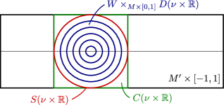
Figure 14. The stabilization $\mathrm{St}^{e}(\bar{W})$ for an embedding $e\colon M\to M^{\prime}$.

Note that Lemma 5.12 applies also to this extended stabilization. Let $C$ be the complement of the image of the interior of $D(\nu)$. The trivial region now means the union of $C\times[-1,1]$ and $C(\nu\times\mathbb{R})$. The image of the nontrivial region under $\mathrm{St}^{e}\rho$ is still $D(\nu\times\mathbb{R})\subseteq M^{\prime}\times[-1,1]$, while the image of the trivial region under $\mathrm{St}^{e}\rho$ is the complement of the interior of this disc bundle.

We will also need the following functoriality property of stabilization with respect to isomorphisms, which is easy to check from the definitions.

Lemma 5.17.

Each encased diffeomorphism $f\colon W\xrightarrow{\cong}W^{\prime}$ of $h$-cobordisms over $M$ (Definition 4.4) induces an encased diffeomorphism

$$\mathrm{St}^{e}(f)\colon\mathrm{St}^{e}(\bar{W})\xrightarrow{\cong}\mathrm{St}^{e}(\bar{W}^{\prime})$$

of $h$-cobordisms over $M^{\prime}$.

5.3. Iterated stabilization

Now assume that we have two composable embeddings of compact $G$-manifolds with corners

$$M_{0}\to M_{1}\to M_{2}$$

extending to codimension 0 embeddings

$$e_{01}\colon D(\nu_{01})\to M_{1},\quad e_{12}\colon D(\nu_{12})\to M_{2},\quad e_{02}\colon D(\nu_{02})\to M_{2}$$

where the various $D(\nu_{ij})$ are smooth $G$-equivariant round bundles

$$D(\nu_{01})\to M_{0},\quad D(\nu_{12})\to M_{1},\quad D(\nu_{02})\to M_{0}$$

and the embedding $e_{02}$ identifies $D(\nu_{02})$ with the round composite of

In this setup we will define a bijection $\mathrm{St}^{e_{12}}\mathrm{St}^{e_{01}}(\bar{W})\cong\mathrm{St}^{e_{02}}(\bar{W})$ and prove it is a diffeomorphism.

Proposition 5.18.

There is a canonical natural homeomorphism

$$\mathrm{St}^{e_{12}}\mathrm{St}^{e_{01}}(\bar{W})\cong\mathrm{St}^{e_{02}}(\bar{W}).$$

The map will preserve the encasing function, and it will also preserve the associated point in $W$, when it exists. By Lemma 5.12, there is at most one map with this property, so we are really just claiming that such a map exists and is a homeomorphism. The canonical map is also natural with respect to isomorphisms, meaning that for each encased diffeomorphism $f\colon W\xrightarrow{\cong}W^{\prime}$ the following square commutes.

Proof.

We begin by identifying the trivial regions. The trivial region of $\mathrm{St}^{e_{01}}(\bar{W})$ consists of all points that go to the complement of the interior of $D(\nu_{01}\times\mathbb{R})$ in $M_{1}\times[-1,1]$. If we apply Corollary 5.15 to an open neighborhood of this first trivial region, we conclude that $\mathrm{St}^{e_{12}}\mathrm{St}^{e_{01}}\rho$ is a diffeomorphism on an “extended trivial region” in the double stabilization $\mathrm{St}^{e_{12}}\mathrm{St}^{e_{01}}(\bar{W})$, consisting of both the complement of the interior of $D(\nu_{12}\times\mathbb{R})$ in $M_{2}\times[-1,1]$, and those points in

$$\mathrm{St}^{e_{01}}(W)\times_{M_{1}\times[0,1]}D(\nu_{12}\times\mathbb{R})$$

where the first coordinate in $\mathrm{St}^{e_{01}}(W)$ is in the first trivial region. This hits all the points in $D(\nu_{12}\times\mathbb{R})$ except those in the image of

$$D(\nu_{01}\times[0,1])\times_{D(\nu_{01})\times[0,1]}D(\nu_{12}\times\mathbb{R})|_{D(\nu_{01})},$$

mapping to $D(\nu_{12}\times\mathbb{R})\subseteq M_{2}\times[-1,1]$ by projection. The map sends $(v,|u|,u)$ to $(v,u)$, so if we regard the restricted disc bundle as a product

$$D(\nu_{12}\times\mathbb{R})|_{D(\nu_{01})}\cong D(\nu_{01})\times D(\nu_{12}\times\mathbb{R})$$

then the map hits all pairs $(v,u)$ such that $|v|^{2}+|u|^{2}<1$. In other words, the extended trivial region is identified with the complement of the interior of $D(\nu_{02}\times\mathbb{R})$. However this is exactly the same set of points that are identified with the trivial region in $\mathrm{St}^{e_{02}}(\bar{W})$. We conclude there is a unique identification between the extended trivial region in $\mathrm{St}^{e_{12}}\mathrm{St}^{e_{01}}(\bar{W})$ and the trivial region in $\mathrm{St}^{e_{02}}(\bar{W})$ that commutes with the encasing functions.

For the nontrivial regions, we pick a trivialization of $D(\nu_{12})$ along the fibers of $D(\nu_{01})$, so that we can regard $D(\nu_{02})$ as the disc inside a direct sum round bundle $D(\nu_{01}\oplus\nu_{12})$. We take the map of fiber products

(19)

Here $v\in\nu_{01}$, $t\in[0,1]$, and $u\in\nu_{12}\times\mathbb{R}$. This map satisfies Lemma 5.12 because it preserves the associated point in $W$, and the encasing functions take each side to

$$(v,\ u)\in D(\nu_{01})\times D(\nu_{12}\times\mathbb{R})\subseteq M_{2}\times[-1,1].$$

It is also a bijection with inverse $(w,v,u)\mapsto(w,v,|u|,u)$.

All together this gives the canonical bijection $\mathrm{St}^{e_{12}}\mathrm{St}^{e_{01}}(\bar{W})\cong\mathrm{St}^{e_{02}}(\bar{W})$. It is clearly continuous, and since the source is compact it is also a homeomorphism. ∎

We note the following associative property of the canonical homeomorphism.

Lemma 5.20.

For any composite of three embeddings with tubular neighborhoods, the iterated stabilization maps fit into a commutative square

Here the bottom horizontal map is the canonical isomorphism from Proposition 5.18, applied to the cobordism $\mathrm{St}^{e_{01}}\bar{W}$, and the right vertical map is the isomorphism from Lemma 5.17 induced on the stabilization $\mathrm{St}^{e_{23}}$ by the canonical isomorphism $\mathrm{St}^{e_{02}}\bar{W}\cong\mathrm{St}^{e_{12}}\mathrm{St}^{e_{01}}\bar{W}$.

Proof.

This follows easily from the defining property of the canonical homeomorphism of Proposition 5.18. ∎

Lastly, we prove that the iterated stabilization map is a diffeomorphism with respect to the smooth structures we defined on the stabilizations.

Theorem 5.21.

The canonical homeomorphism

$$\mathrm{St}^{e_{12}}\mathrm{St}^{e_{01}}(\bar{W})\cong\mathrm{St}^{e_{02}}(\bar{W})$$

is an encased diffeomorphism.

Proof.

We already know this homeomorphism commutes with the encasing functions. The fact that it is a diffeomorphism between the extended trivial region in $\mathrm{St}^{e_{12}}\mathrm{St}^{e_{01}}(\bar{W})$ and the trivial region in $\mathrm{St}^{e_{02}}(\bar{W})$ follows because the encasing functions are diffeomorphisms on those regions (and so the canonical homeomorphism is a composite of two diffeomorphisms).

It remains to show that the canonical homeomorphism is smooth and full-rank inside the nontrivial region, where it is given by (19). Since the check is local and the smooth charts are defined by trivializing the bundles, without loss of generality the bundles are trivial, so the map to check is

(22)

The points in the nontrivial region can be divided into three cases.

Case 1: Points not in the cone locus of $\mathrm{St}^{e_{12}}$. These are the points $(w,v,t,u)$ for which $t\neq 0$, and therefore also $u\neq 0$ and $w\not\in N$. Both fiber products on the left-hand side of (22) are being taken over $(0,1)$ here, where the map on the right is a submersion and the smooth structure on the fiber product is being inherited from the product. Smoothness is therefore clear. The inverse has formula $(w,v,u)\mapsto(w,v,|u|,u)$, which is also smooth since $|u|>0$. Therefore the map has full rank at these points as well.

Case 2: Points in the cone locus of $\mathrm{St}^{e_{12}}$ but not also in the cone locus of $\mathrm{St}^{e_{02}}$. These are the points $(w,v,t,u)$ for which $t=0$ and therefore $u=0$, but $w\not\in N$. On the left-hand side of (22) this means the first fiber product is over $(0,1)$ but the second is at 0.

We adopt the shorthand

$$W_{0}=W\setminus(M\amalg N),\qquad D_{0}=D\setminus(\{0\}\cup\partial D),$$

$$N_{1}=W_{0}\times_{(0,1)}D_{0}(V_{1}),\qquad\bar{W}_{1}=W_{0}\times_{(0,1)}D_{0}(V_{1}\times\mathbb{R}).$$

So $N_{1}$ is the top of $\mathrm{St}^{\nu_{01}}(W)$ minus the cone locus and frontier, and $\bar{W}_{1}$ is a neighborhood of $N_{1}$ in $\mathrm{St}^{\nu_{01}}(\bar{W})$. We choose the bicollar for $N_{1}$ in $\bar{W}_{1}$ by the formula

As interpreted strictly, this is not defined on the entire domain, but we interpret it as defined near an arbitrary point in the domain for small enough $\epsilon$. It is equivariant and full-rank and therefore defines an equivariant bicollar.

The chart from Definition 5.9 that gives the smooth structure on $\mathrm{St}^{\nu_{12}}$ is the composite of the first two maps below. The remaining map below is the canonical homeomorphism.

The composite is (a restriction of) an identity map, so it is smooth and full rank.

Case 3: Points in the cone locus of both $\mathrm{St}^{e_{01}}$ and $\mathrm{St}^{e_{02}}$. These are the points $(w,v,t,u)=(n_{0},0,0,0)$ with $n_{0}\in N$. From Definition 5.9, the smooth structure on $\mathrm{St}^{e_{01}}(W)$ near one such point is defined by taking a neighborhood $U$ of $n_{0}$ in $N$ and $(G\times C_{2})$-equivariant bicollar $b\colon U\times(-\epsilon,\epsilon)\to\bar{W}$. The smooth chart has the formula

Inside this smooth chart, the top of the cobordism is identified with the subset $U\times D(V_{1})$. This top has a bicollar that is the inclusion (defined sufficiently close to the center of $D(V_{1})$)

$$c\colon U\times D(V_{1})\times(-\epsilon,\epsilon)\subseteq U\times D(V_{1}\times\mathbb{R}).$$

In the following diagram, the top horizontal is the canonical homeomorphism. The left-hand column is the smooth chart on the double stabilization $\mathrm{St}^{e_{12}}\mathrm{St}^{e_{01}}(\bar{W})$, obtained by taking the smooth chart on the first stabilization defined just above using $b$, and then defining the smooth structure on the second stabilization inside that chart using $c$. The right-hand column is the smooth chart in the single stabilization $\mathrm{St}^{e_{02}}(\bar{W})$, defined using the same bicollar $b$.

The top horizontal has the formula $(w,v,t,u)$ to $(w,v,u)$ as in (22). On the second line we can define the dashed map in the same way, replacing $w$ by $(n,s)$, which makes the top square commute. On the third line we similarly send $(n,y,t,u)$ to $(n,y,u)$, making the second square commute:

Therefore the canonical homeomorphism, in these charts, is given by the lower route of the diagram:

This is just the identity map (restricted to a neighborhood of zero), which is obviously smooth and full-rank. ∎

5.4. Stabilizing a family

If $E\to\Delta^{k}$ is a family of encased $h$-cobordisms over $M$, then we can regard it as a cobordism over $M\times\Delta^{k}$. Given a round bundle $D(\nu)\to M\times\Delta^{k}$, we can apply the procedure of Definition 5.7 to the cobordism $E$ to produce a cobordism $\mathrm{St}^{\nu}(E)$ over $D(\nu)\times\Delta^{k}$. Given a $k$-simplex of tubular neighborhoods $e\colon D(\nu)\to M^{\prime}\times\Delta^{k}$, we then extend by zero to produce a cobordism $\mathrm{St}^{e}(E)$ over $M^{\prime}\times\Delta^{k}$.

The one difference in this case is that $E$ is not trivial over $M\times\partial\Delta^{k}$, only over $\partial M\times\Delta^{k}$. However, we only need $\mathrm{St}^{e}(E)$ to be trivial on $\partial M^{\prime}\times\Delta^{k}$, not $M^{\prime}\times\partial\Delta^{k}$. So the collar of $\mathrm{St}^{e}(E)$ only has to be defined near the bottom $M^{\prime}\times\Delta^{k}\times\{0\}$ and the part of the sides corresponding to $\partial M^{\prime}\times\Delta^{k}\times I$, and indeed it is using Lemma 5.14.

We have to establish the following lemma, so that by Lemma 2.21 the stabilization $\mathrm{St}^{e}(\bar{E})$ is a smooth fiber bundle over $\Delta^{k}$, as required by Definition 4.7.

Proposition 5.23.

If $E\to\Delta^{k}$ is a submersion then so is $\mathrm{St}^{e}(\bar{E})\to\Delta^{k}$.

Proof.

As this is a local statement, we can assume that $E=W\times\Delta^{k}$ and the bundle $\nu$ is trivial, but we cannot assume that the encasing function is constant. On an open neighborhood of the trivial region, the map is identified with a product projection

$$M^{\prime}\times\Delta^{k}\times[-1,1]\to\Delta^{k}$$

and is therefore a submersion.

On the interior of the nontrivial region minus the cone locus, we can ignore the $C_{2}$ quotient, and since $S(V\times\Delta^{k})\to M\times\Delta^{k}$ and $\bar{W}\times\Delta^{k}\to\Delta^{k}$ are submersions, so is the map

$$((\bar{W}\setminus N)\times\Delta^{k})\times_{(M\times\Delta^{k})}S(V\times\Delta^{k})\to\Delta^{k}.$$

The fact that the retraction $r\colon\bar{W}\to M$ is not a submersion does not interfere with this.

Finally, on any chart at the cone locus

$$U\times\Delta^{k}\times D(V\times\mathbb{R}),$$

in which we have chosen the bicollar $U\times\Delta^{k}\times(-\epsilon,\epsilon)\to\bar{W}\times\Delta^{k}$ to be fiberwise over $\Delta^{k}$, the map to $\Delta^{k}$ is just the projection, so it is a submersion here as well. ∎

For definiteness, each cobordism $W$ is a subset of some sufficiently large set $\mathcal{U}$, and for the stabilization procedure we fix a way of assigning the stabilized cobordism $\mathrm{St}^{e}(W)$ to another subset of $\mathcal{U}$. Each family $E\to\Delta^{k}$ is then considered as a subset of $\mathcal{U}\times\Delta^{k}$ – this guarantees that restricting to a face or pulling back along a degeneracy strictly commutes with stabilization. As a result we get a map of spaces

$$\mathrm{St}^{e}\colon\mathcal{H}_{\,\begin{picture}(-1.0,1.0)(0.5,-1.0)\circle*{1.8}\end{picture}\hskip 1.42271pt}^{c}(M)\to\mathcal{H}_{\,\begin{picture}(-1.0,1.0)(0.5,-1.0)\circle*{1.8}\end{picture}\hskip 1.42271pt}^{c}(M^{\prime}).$$

For two stabilizations, the canonical homeomorphism $\mathrm{St}^{e_{01}}\mathrm{St}^{e_{12}}(\bar{E})\cong\mathrm{St}^{e_{02}}(\bar{E})$ has the same definition as before over each point of $\Delta^{k}$. As the formulas are built using functions that are smooth on all of $E$, the results are still smooth, and full-rank whenever they are full-rank over each point of $\Delta^{k}$ separately (because the derivative is the identity in the $\Delta^{k}$ direction). The canonical homeomorphism is therefore a diffeomorphism of manifolds over $\Delta^{k}$.

One can directly construct out of this a homotopy

$$\mathrm{St}^{e_{01}}\mathrm{St}^{e_{12}}\sim\mathrm{St}^{e_{02}}\colon\mathcal{H}_{\,\begin{picture}(-1.0,1.0)(0.5,-1.0)\circle*{1.8}\end{picture}\hskip 1.42271pt}^{c}(M_{0})\times I\to\mathcal{H}_{\,\begin{picture}(-1.0,1.0)(0.5,-1.0)\circle*{1.8}\end{picture}\hskip 1.42271pt}^{c}(M_{2}).$$

This makes $\mathcal{H}_{\,\begin{picture}(-1.0,1.0)(0.5,-1.0)\circle*{1.8}\end{picture}\hskip 1.42271pt}^{c}$ (and therefore $\mathcal{H}_{\,\begin{picture}(-1.0,1.0)(0.5,-1.0)\circle*{1.8}\end{picture}\hskip 1.42271pt}$) into a functor from the homotopy category of manifolds and smooth embeddings to the homotopy category of spaces. (Note the choice of tubular neighborhood $D(\nu)\to M^{\prime}$ is contractible by Theorem 2.19, making the induced maps well-defined up to homotopy.) In the next section, we do this in a more structured way and get a functor up to coherent homotopy.

6. The $h$-cobordism space as an $(\infty,1)$-functor

Now that we have most of the geometric preliminaries out of the way, we review a categorical framework to construct $(\infty,1)$-functors using Segal spaces, following [BdB18, Ras17]. We then build the smooth $h$-cobordism functor using this setup.

6.1. Left fibrations of Segal spaces

We start by recalling the basic definitions. In this section any time we say “space” we mean simplicial set.

Definition 6.1.

A Segal space is a simplicial space $X_{\,\begin{picture}(-1.0,1.0)(0.5,-1.0)\circle*{1.8}\end{picture}\hskip 1.42271pt}$ (i.e. a bisimplicial set) such that the derived Segal maps

are weak equivalences. An important special case is a Segal category, which is a Segal space with $X_{0}$ discrete.

Nerves of simplicially enriched categories are always Segal spaces, as are nerves of categories internal to simplicial sets, provided the source or target map $X_{1}\to X_{0}$ is a fibration.

In contrast to much of the literature on Segal spaces, following [BdB18], we do not assume that our Segal spaces are Reedy fibrant. This will be convenient for the examples we aim to build.

Definition 6.2.

Let $B$ be a Segal space. A left fibration over $B$ is a map of simplicial spaces $X\to B$ such that $X$ is also a Segal space, and the square

is homotopy cartesian. By [BdB18, 1.7], in lieu of checking that $X$ is a Segal space, we could alternatively check that for each $n>0$ the square

is homotopy cartesian.

Let $\mathcal{F}_{B}$ denote the category of left fibrations over the Segal space $B$. A weak equivalence of Segal spaces is a levelwise equivalence, i.e. $X_{n}\to Y_{n}$ is an equivalence of spaces for all $n$. Inverting these weak equivalences on the category of left fibrations over $B$, gives a homotopy category of left fibrations over $B$, which we denote $ho\mathcal{F}_{B}$.

Proposition 6.3.

Any weak equivalence of Segal spaces $B^{\prime}\to B$ induces an equivalence on homotopy categories of fibrations $ho\mathcal{F}_{B^{\prime}}\simeq ho\mathcal{F}_{B}$.

In fact, the homotopy category $ho\mathcal{F}_{B}$ comes from a model structure on the category $ssSet_{B}$ of all simplicial spaces over $B$, described in [BdB18, Proposition 1.10], and any weak equivalence of Segal spaces induces a Quillen equivalence. We can see the equivalence of homotopy categories from Proposition 6.3 quite easily though:

A left fibration $X\to B$ is fibrant if the maps $X_{n}\to B_{n}$ are Kan fibrations. If $B^{\prime}\to B$ is any weak equivalence of Segal spaces, the pullback of any fibrant left fibration $X$ over $B$ to $B^{\prime}$ is a left fibration, see [BdB18, 1.11]. We therefore get a functor $\mathcal{F}_{B}\to\mathcal{F}_{B^{\prime}}$. This functor preserves weak equivalences between fibrant left fibrations over $B$, giving a functor $ho\mathcal{F}_{B}\to ho\mathcal{F}_{B^{\prime}}$. The left adjoint $\mathcal{F}_{B^{\prime}}\to\mathcal{F}_{B}$ sends each left fibration $X^{\prime}\to B^{\prime}$ to the composite $X^{\prime}\to B^{\prime}\to B$. This is always a Segal space, and is a left fibration as well under the assumption that $B^{\prime}\to B$ is a weak equivalence. It is easy to see that the derived functors of this adjunction give an equivalence of homotopy categories $ho\mathcal{F}_{B^{\prime}}\simeq ho\mathcal{F}_{B}$.

We will rely on the following result from [BdB18, Ras17], which we restate in terms of left instead of right fibrations.

Theorem 6.4.

Let $\mathcal{C}$ be a simplicially enriched category. There exists a Quillen equivalence

$$\textup{ssSet}_{/N\mathcal{C}}\leftrightarrows\textup{Fun}(\mathcal{C},\textup{sSet}),$$

where the category of bisimplicial sets ssSet over $N\mathcal{C}$ is endowed with the left fibration model structure, and the functor category is endowed with the projective model structure.

Along this equivalence, each left fibration $X\to N\mathcal{C}$ is sent to a diagram in which the objects and morphisms can be described explicitly up to homotopy. Let $X(c)$ be the pullback $X_{0}\times_{(N\mathcal{C})_{0}}\{c\}$, in other words the subspace of $X_{0}$ lying over the object $c$. Note that

$$X_{0}=\coprod_{c}X(c),$$

and the left fibration condition on $X$ gives canonical weak equivalences

(5)

In particular, for $n=1$ we get a canonical zig-zag

(6)

This gives an action-up-to-homotopy of the morphism space $\mathcal{C}(c,d)$ on the space $X(c)$.

Lemma 6.7.

The equivalence of Theorem 6.4 sends each left fibration $X\to N\mathcal{C}$ to a diagram whose value at $c$ is equivalent to $X(c)$, and for which the action of $\mathcal{C}(c,d)$ is in the same homotopy class as the zig-zag (6).

Proof.

The description we gave of the objects and the actions is invariant under weak equivalence of left fibrations. Furthermore, each left fibration is equivalent to one coming from a diagram on $\mathcal{C}$. Therefore without loss of generality, $X$ arose from a diagram on $\mathcal{C}$ by applying the right adjoint functor from Theorem 6.4.

Explicitly, this right adjoint takes a diagram with spaces $X(c)$ and forms a simplicial space by the categorical bar construction. In other words, the maps (5) are isomorphisms. Furthermore the action of $d_{1}$ in (6) is by the action of $\mathcal{C}$ on the diagram $X(-)$. This verifies the claim in this special case, and therefore in general as well. ∎

Remark 6.8.

The equivalence does not take all points in $X_{n}$ for each $n$ that project to $n$ copies of the identity map in $(N\mathcal{C})_{n}$. In other words, it does not take “everything projecting to an identity map in $\mathcal{C}$,” only the subspaces of $X_{0}$ that project to each object in $\mathcal{C}$.

Using this machinery, our strategy will be as follows: we construct a simplicial category $\mathcal{M}^{\mathrm{Stab}}$ of manifolds and stabilization data, and show it is equivalent to the simplicial category $\mathcal{M}^{\mathrm{Emb}}$ of manifolds and smooth embeddings. We then construct a left fibration $X\to N\mathcal{M}^{\mathrm{Stab}}$, such that $X_{0}$ is the disjoint union of the $h$-cobordism spaces $\mathcal{H}_{\,\begin{picture}(-1.0,1.0)(0.5,-1.0)\circle*{1.8}\end{picture}\hskip 1.42271pt}^{c}(M)$, and the actions coming from $X_{1}$ are the required stabilization maps, up to homotopy. Applying Lemma 6.7, produces the desired $h$-cobordism functor on $\mathcal{\mathcal{M}^{\mathrm{Emb}}}$.

6.2. The category of smooth manifolds and tubular neighborhoods

Definition 6.9.

Let $\mathcal{M}^{\mathrm{Sm}}$ refer to the category of smooth compact $G$-manifolds with corners, and smooth equivariant maps. The morphisms from $M_{0}$ to $M_{1}$ are the simplicial set $\mathrm{Sm}(M_{0},M_{1})$ whose $p$-simplices are equivariant smooth maps

$$M_{0}\times\Delta^{p}\to M_{1}.$$

Let $\mathcal{M}^{\mathrm{Emb}}$ refer to the subcategory with the same objects, but where the morphism spaces are restricted to the subspace

$$\mathrm{Emb}(M_{0},M_{1})\subseteq\mathrm{Sm}(M_{0},M_{1})$$

of those smooth maps that are smooth embeddings.

One can show that these mapping spaces are Kan complexes, equivalent to the singular simplices of the spaces of smooth maps or of embeddings with the $C^{\infty}$ topology.

Definition 6.10.

The category of manifolds and stabilization data $\mathcal{M}^{\mathrm{Stab}}$ is a category enriched in simplicial sets, described as follows. The objects are smooth compact $G$-manifolds with corners. A map from $M_{0}$ to $M_{1}$ is given by a round bundle $p_{0}\colon D(\nu_{01})\to M_{0}$ and an embedding $e_{01}\colon D(\nu_{01})\hookrightarrow M_{1}$. The round bundles are considered up to isomorphism of the bundles commuting with the embeddings.

Given another morphism from $M_{1}$ to $M_{2}$ defined by a round bundle $p_{12}\colon D(\nu_{12})\to M_{1}$ and embedding $e_{12}\colon D(\nu_{12})\hookrightarrow M_{2}$, we define the composite map from $M_{0}$ to $M_{2}$ by taking the subspace $D(\nu_{02})$ of the pullback

(11)

consisting of points $(s,t)$ such that $s^{2}+t^{2}\leq 1$. This is a round bundle $p_{02}\colon D(\nu_{02})\to M_{0}$, and it has an embedding $e_{02}\colon D(\nu_{02})\hookrightarrow M_{2}$. Note that this composition is associative.

We simplicially enrich $\mathcal{M}^{\mathrm{Stab}}$ by defining a $p$-simplex of morphisms from $M_{0}$ to $M_{1}$ to be a round bundle $D(\nu_{01})\to M_{0}\times\Delta^{p}$ with a codimension 0 embedding $D(\nu_{01})\to M_{1}\times\Delta^{p}$ over $\Delta^{p}$. The composition map is then a map of simplicial sets.

Theorem 6.12.

The map that forgets the stabilization data is an equivalence of simplicial categories $\mathcal{M}^{\mathrm{Stab}}\to\mathcal{M}^{\mathrm{Emb}}$.

Proof.

Applying Proposition 2.23 to $N$, we can deform any $\Delta^{p}$ family of embeddings $M\to N$ to a family of embeddings that all lie in the interior of $N$. Furthermore, if the embeddings along $\partial\Delta^{p}$ already lie in the interior of $N$, then this homotopy can be done rel $\partial\Delta^{p}$. Therefore, if we restrict the mapping spaces $\mathcal{M}^{\mathrm{Emb}}(M,N)$ to those embeddings that land in the interior of the target, we get an equivalent Kan complex. Similarly, restricting $\mathcal{M}^{\mathrm{Stab}}(M,N)$ to the data where $D(\nu)\to N$ lands in the interior of $N$, gives an equivalent simplicial set that is a Kan complex. Now the result follows from Theorem 5.6, the tubular neighborhood theorem for round bundles. ∎

Remark 6.13.

We do not prove that the mapping spaces $\mathcal{M}^{\mathrm{Stab}}(M,N)$ are Kan complexes. This would be easy to prove if we made $D\nu\to N$ always land in the interior of $N$. However the stabilization from Definition 5.16 works just fine even if $D\nu$ touches $\partial N$, and this occurs frequently in examples. So it is a little more convenient in our setup if $\mathcal{M}^{\mathrm{Stab}}$ allows all embeddings $D\nu\to N$.

6.3. The homotopy coherent $h$-cobordism functor

The next step is to define the desired left fibration over $N\mathcal{M}^{\mathrm{Emb}}$. By Proposition 6.3 and Theorem 6.12, it suffices to build the left fibration over $N\mathcal{M}^{\mathrm{Stab}}$ instead.

Definition 6.14.

We define $\mathcal{H}^{\mathrm{Stab}}$ as the following category internal to simplicial sets. The simplicial set of objects is $\coprod_{M}\mathcal{H}_{\,\begin{picture}(-1.0,1.0)(0.5,-1.0)\circle*{1.8}\end{picture}\hskip 1.42271pt}^{c}(M)$, the space of all encased $h$-cobordisms over all compact $G$-manifolds with corners $M$. A $0$-simplex of morphisms from an $h$-cobordism $W_{0}$ on $M_{0}$ to an $h$-cobordism $W_{1}$ on $M_{1}$ is a morphism in $\mathcal{M}^{\mathrm{Stab}}$ from $M_{0}$ to $M_{1}$ together with an encased diffeomorphism $f_{01}\colon\mathrm{St}^{e_{01}}\bar{W}_{0}\cong\bar{W}_{1}$.

Given another morphism from $W_{1}$ to an $h$-cobordism $W_{2}$ on $M_{2}$, and encased diffeomorphism $f_{12}\colon\mathrm{St}^{e_{12}}\bar{W}_{1}\cong\bar{W}_{2}$, we define the composite morphism from $W_{0}$ to $W_{2}$ as follows. We compose the morphisms in $\mathcal{M}^{\mathrm{Stab}}$, and define the encased diffeomorphism $f_{02}\colon\mathrm{St}^{e_{02}}\bar{W}_{0}\cong W_{2}$ as

(15) $$\mathrm{St}^{e_{02}}\bar{W}_{0}\xrightarrow[\cong]{}\mathrm{St}^{e_{12}}\mathrm{St}^{e_{01}}\bar{W}_{0}\xrightarrow[\cong]{\mathrm{St}^{e_{12}}(f_{01})}\mathrm{St}^{e_{12}}\bar{W}_{1}\xrightarrow[\cong]{f_{12}}\bar{W}_{2},$$

where the first unlabeled diffeomorphism is the canonical isomorphism of Proposition 5.18. We show associativity in the next lemma.

A $p$-simplex of morphisms in $\mathcal{H}^{\mathrm{Stab}}$ is a $p$-simplex in $\mathcal{M}^{\mathrm{Stab}}$ from $M_{0}$ to $M_{1}$ together with an encased diffeomorphism of families $f_{01}\colon\mathrm{St}^{e_{01}}\bar{E}_{0}\cong\bar{E}_{1}$ over $\Delta^{p}$. The composition is defined in the same was as above. The source, target, and composition maps are all maps of simplicial sets.

Lemma 6.16.

The composition rule for $\mathcal{H}^{\mathrm{Stab}}$ defined in Definition 6.14 is associative.

Proof.

We consider the associativity of composition on 0-simplices of the morphism simplicial set, since on $p$-simplices the argument is similar.

Suppose we are given morphisms $M_{0}\to M_{1}\to M_{2}\to M_{3}$ in $\mathcal{H}^{\mathrm{Stab}}$. First, this is the data of such morphisms in $\mathcal{M}^{\mathrm{Stab}}$, which is a diagram of round bundle composites

We recall that this composition in $\mathcal{M}^{\mathrm{Stab}}$ is strictly associative. Moreover, we are given the data of isomorphisms

$$\mathrm{St}^{e_{01}}\bar{W}_{0}\xrightarrow[\cong]{f_{01}}\bar{W}_{1},\ \ \ \ \mathrm{St}^{e_{12}}\bar{W}_{1}\xrightarrow[\cong]{f_{12}}\bar{W}_{2},\ \ \ \ \mathrm{St}^{e_{23}}\bar{W}_{2}\xrightarrow[\cong]{f_{23}}\bar{W}_{3}.$$

The two ways of associating the three-fold composition are given by the top and bottom routes of the following diagram, from $\mathrm{St}^{e_{03}}\bar{W}_{0}$ to $W_{3}$. The left-hand square commutes by Lemma 5.20 and the middle square commutes by Proposition 5.18. This verifies associativity in $\mathcal{H}^{\mathrm{Stab}}$.

∎

Since $\mathcal{H}^{\mathrm{Stab}}$ is a category internal to simplicial sets, its nerve is a strict Segal space. It will be a consequence of Proposition 6.17 below that it is also a (homotopical) Segal space.

There is an evident forgetful map of simplicial categories $\mathcal{H}^{\mathrm{Stab}}\to\mathcal{M}^{\mathrm{Stab}}$, and therefore a map of bisimplicial sets $N\mathcal{H}^{\mathrm{Stab}}\to N\mathcal{M}^{\mathrm{Stab}}$, that forgets the $h$-cobordism but remembers the base manifold.

Proposition 6.17.

The map $N\mathcal{H}^{\mathrm{Stab}}\to N\mathcal{M}^{\mathrm{Stab}}$ is a left fibration.

Proof.

By Definition 6.2, it suffices to show that the morphism spaces, object spaces, and source maps define a homotopy pullback square:

In the right-hand column, the target $\mathcal{M}^{\mathrm{Stab}}_{0}$ is discrete, the set of all compact $G$-manifolds with corners $M$. Each fiber of the map $\mathcal{H}^{\mathrm{Stab}}_{0}\to\mathcal{M}^{\mathrm{Stab}}_{0}$ is a space of encased equivariant $h$-cobordisms $\mathcal{H}_{\,\begin{picture}(-1.0,1.0)(0.5,-1.0)\circle*{1.8}\end{picture}\hskip 1.42271pt}^{c}(M)$. By Proposition 4.12, these fiber spaces are Kan complexes, so the right-hand vertical is a Kan fibration. Therefore it suffices to show that the map from $\mathcal{H}^{\mathrm{Stab}}_{n}$ to the strict pullback is an acyclic Kan fibration.

We prove this first when $n=1$. The claim is that if we have a $p$-simplex of morphisms $e\colon M_{0}\to M_{1}$ in $N\mathcal{M}^{\mathrm{Stab}}$, a family $E_{0}$ of $h$-cobordisms over $M_{0}\times\Delta^{p}$ that restricts to a family $\partial E_{0}$ over $M_{0}\times\partial\Delta^{p}$, a family of $h$-cobordisms $\partial E_{1}$ on $M_{1}\times\partial\Delta^{p}$, and a diffeomorphism $\partial E_{1}\cong\mathrm{St}^{e}(\partial E_{0})$, then this data can be extended to a family $E_{1}$ on $M_{1}\times\Delta^{p}$ and a diffeomorphism $E_{1}\cong\mathrm{St}^{e}(E)$. This is easy – we form $E_{1}$ by taking $\mathrm{St}^{e}(E)$, and applying a bijection to the underlying set along $M_{1}\times\partial\Delta^{p}$, so that the points in that subset are replaced by the corresponding points in the original family $\partial E_{1}$.

For $n>1$ the proof is the same, except that we have a $p$-simplex of composable morphisms $M_{0}\to M_{1}\to\cdots\to M_{n}$, a family $E_{0}$ over $M_{0}\times\Delta^{p}$, and the restricted family $\partial E_{0}$ over $M_{0}\times\partial\Delta^{p}$ is stabilized to each $M_{i}$ and identified with some family $\partial E_{i}$ over $M_{i}\times\partial\Delta^{p}$, for each $i$. Again, we extend this to a full family $E_{i}$ over $M_{i}\times\Delta^{p}$ by stabilizing all of $E_{0}$, and relabeling the points over $\partial\Delta^{p}$ to match the original given family $\partial E_{i}$. ∎

Applying Lemma 6.7 to this left fibration gives the main theorem of the paper.

Theorem 6.18.

There is a functor

$$\mathcal{H}_{\,\begin{picture}(-1.0,1.0)(0.5,-1.0)\circle*{1.8}\end{picture}\hskip 1.42271pt}(-)\colon\mathcal{M}^{\mathrm{Emb}}\to\textup{sSet}\,,$$

sending each compact $G$-manifold with corners $M$ to a space equivalent to $\mathcal{H}_{\,\begin{picture}(-1.0,1.0)(0.5,-1.0)\circle*{1.8}\end{picture}\hskip 1.42271pt}(M)$, and each homotopy class of smooth equivariant embeddings $M\to M^{\prime}$ to the homotopy class of maps $\mathcal{H}_{\,\begin{picture}(-1.0,1.0)(0.5,-1.0)\circle*{1.8}\end{picture}\hskip 1.42271pt}(M)\to\mathcal{H}_{\,\begin{picture}(-1.0,1.0)(0.5,-1.0)\circle*{1.8}\end{picture}\hskip 1.42271pt}(M^{\prime})$ given by the stabilization in Section 5.

7. The stable $h$-cobordism space

Now that we have made the space of equivariant $h$-cobordisms into a functor on smooth manifolds and smooth embeddings, the last task is to stabilize with respect to representation discs, and extend the functor to all $G$-CW complexes and continuous maps. Let $\mathcal{H}(-)$ denote a fixed model for the smooth $h$-cobordism space, as a strict functor from $\mathcal{M}^{\mathrm{Emb}}$ to sSet, using Theorem 6.18. Let $\mathcal{U}$ be a complete $G$-universe.

Definition 7.1.

Let

$$\mathcal{H}^{\mathcal{U}}(M)=\mathcal{H}(M\times\mathcal{U})=\underset{\textup{compact }K\subseteq M\times\mathcal{U}}{\textup{colim}\,}\ \ \mathcal{H}(K)$$

be the space (simplicial set) obtained as the colimit over inclusions of compact $G$-invariant submanifolds of $M\times\mathcal{U}$. When $G=1$ we also refer to this as $\mathcal{H}^{\infty}(M)$.

Since colimits are natural, $\mathcal{H}^{\mathcal{U}}(-)$ is also a functor on the category $\mathcal{M}^{\mathrm{Emb}}$ of compact smooth $G$-manifolds and embeddings.

Remark 7.2.

By cofinality, this colimit can be evaluated by taking only the submanifolds of the form $M\times D_{R}(V)$ for finite-dimensional representations $V\subseteq\mathcal{U}$, and $R\geq 1$ a radius that goes to infinity. Since $M\times D(V)\to M\times D_{R}(V)$ is homotopic through embeddings to a diffeomorphism, it induces an equivalence on $\mathcal{H}(-)$, and therefore we have an equivalence from the colimit over representation discs,

Remark 7.3.

Also by cofinality, the colimit can be evaluated by taking only the submanifolds of $M\times\mathcal{U}$ that are framed, or stably framed. Intuitively, this means that $\mathcal{H}^{\mathcal{U}}(M)$ is the homotopy colimit over “all” stably framed manifolds mapping to $M$, as in [Wal82, p.152].

Our next task is to extend $\mathcal{H}^{\mathcal{U}}(-)$ from the category of embeddings $\mathcal{M}^{\mathrm{Emb}}$ to the larger category of smooth maps $\mathcal{M}^{\mathrm{Sm}}$ from Definition 6.9. To do this, we define the space $\mathrm{Emb}(M_{0},M_{1}\times\mathcal{U})$ as the colimit of the spaces of embeddings into compact submanifolds of $M_{1}\times\mathcal{U}$. Including the origin into $\mathcal{U}$, and projecting away $\mathcal{U}$, induce maps

(4)

whose composite is the inclusion of the space of embeddings into the space of all smooth maps.

Lemma 7.5.

The second map in (4), that projects away $\mathcal{U}$, is a weak equivalence.

Proof.

The argument is similar to that of Theorem 2.19 and Lemma 4.3. Given a $\Delta^{k}$-family of smooth maps $f_{t}\colon M_{0}\to M_{1}$ and $\partial\Delta^{k}$-family of smooth maps $g_{t}\colon M_{0}\to\mathcal{U}$ such that the product maps $(f_{t},g_{t})\colon M_{0}\to M_{1}\times\mathcal{U}$ are embeddings for all $t\in\partial\Delta^{k}$, we need to extend the family $g_{t}$ to all of $\Delta^{k}$ so that the product maps are embeddings for all $t\in\Delta^{k}$.

We first use Lemma 2.14 to extend $g_{t}$ to an open subset $U\subseteq\Delta^{k}$ containing $\partial\Delta^{k}$. The product maps $(f_{t},g_{t})$ are still embeddings provided $U$ is small enough. We shrink $U$ to a closed neighborhood $C$ containing the boundary, whose complement in $\Delta^{k}$ is convex.

Then we extend $g_{t}$ to a continuous family of smooth maps on $\Delta^{k}$, so that $g_{t}$ is an embedding outside of $C$. For instance, by compactness, the maps $g_{t}$ for $t\in C$ all land in a finite-dimensional subspace $V\subseteq\mathcal{U}$, so on $\Delta^{k}\setminus C$ we can linearly interpolate from the embeddings $g_{t}$ for $t\in\partial C$ to a fixed embedding $g$ of $M_{0}$ to the orthogonal complement of $V$ in $\mathcal{U}$. This gives a continuous family of smooth maps $g_{t}\colon M_{0}\to\mathcal{U}$ on $\Delta^{k}$ that are embeddings on $\Delta^{k}\setminus C$, so that the product maps $(f_{t},g_{t})$ are embeddings for all $t\in\Delta^{k}$.

Finally we use smooth approximation (Corollary 2.16) to modify $g_{t}$ away from $\partial\Delta^{k}$ to make the family smooth. Provided the approximation is small enough, the product maps $(f_{t},g_{t})$ are still embeddings for all $t\in\Delta^{k}$. ∎

This motivates us to find an intermediate category $\mathcal{M}^{\mathrm{\mathcal{U}\textup{-}Emb}}$ that is equivalent to $\mathcal{M}^{\mathrm{Sm}}$, but whose morphism spaces involve embeddings of $M_{0}$ into $M_{1}\times\mathcal{U}$. The construction of this category is subtle – we can’t take all embeddings $M_{0}\times\mathcal{U}\to M_{1}\times\mathcal{U}$, because then projecting away $\mathcal{U}$ doesn’t respect composition. On the other hand, we can’t take all maps $M_{0}\to M_{1}\times\mathcal{U}$ and compose them using isometries $\mathcal{U}\times\mathcal{U}\to\mathcal{U}$, because then the category lacks identity maps. The following definition circumvents both of these issues.

Let $\mathcal{L}(\mathcal{U},\mathcal{U})$ be the space of equivariant linear isometries $\mathcal{U}\to\mathcal{U}$, i.e. maps that are equivariant, linear, and metric-preserving, but not necessarily isomorphisms. This is a simplicial set in which a $p$-simplex of linear isometries $\mathcal{U}\times\Delta^{p}\to\mathcal{U}$ must be smooth in the sense that the restriction to $V\times\Delta^{p}$ is smooth for any finite-dimensional subspace $V\subseteq\mathcal{U}$.

Definition 7.6.

The category of manifolds and $\mathcal{U}$-embeddings $\mathcal{M}^{\mathrm{\mathcal{U}\textup{-}Emb}}$ has as objects the smooth compact $G$-manifolds with corners. The morphism space from $M_{0}$ to $M_{1}$ is the subspace

$$\mathcal{M}^{\mathrm{\mathcal{U}\textup{-}Emb}}(M_{0},M_{1})\subseteq\mathcal{L}(\mathcal{U},\mathcal{U})\times\mathrm{Emb}(M_{0},M_{1}\times\mathcal{U})$$

of all isometries $f\colon\mathcal{U}\to\mathcal{U}$ and embeddings $e=(e^{(1)},e^{(2)})\colon M_{0}\to M_{1}\times\mathcal{U}$ such that the second coordinate $e^{(2)}$ lands in the orthogonal complement $f(\mathcal{U})^{\perp}$.

The composition is by composing the isometries $f$, and composing the embeddings $e$ by the rule

It is straightforward to check this is associative and preserves the simplicial structure.

We define functors

that are the identity on objects. The first functor sends each embedding $e\colon M_{0}\to M_{1}$ to the identity $\textup{id}\colon\mathcal{U}\to\mathcal{U}$ and the embedding $(e,0)\colon M_{0}\to M_{1}\times\mathcal{U}$. The second functor sends each pair $f\colon\mathcal{U}\to\mathcal{U}$ and $e=(e^{(1)},e^{(2)})$ to the smooth map $e^{(1)}\colon M_{0}\to M_{1}$. The composite of these functors sends $e\colon M_{0}\to M_{1}$ to itself, forgetting that $e$ is an embedding.

Lemma 7.7.

The stable $h$-cobordism space $\mathcal{H}^{\mathcal{U}}(-)$ extends from $\mathcal{M}^{\mathrm{Emb}}$ to $\mathcal{M}^{\mathrm{\mathcal{U}\textup{-}Emb}}$.

Proof.

From the definition of the functor $\mathcal{H}^{\mathcal{U}}(-)$, it clearly extends to the larger category whose objects are manifolds $M_{0}$, and whose morphisms are embeddings

$$\mathrm{Emb}(M_{0}\times\mathcal{U},M_{1}\times\mathcal{U}).$$

However, this category contains $\mathcal{M}^{\mathrm{\mathcal{U}\textup{-}Emb}}$ inside, by restricting the morphisms to the subset of embeddings of the form

$$(x,v)\mapsto(e^{(1)}(x),f(v)+e^{(2)}(x)).$$

This subcategory, in turn, contains $\mathcal{M}^{\mathrm{Emb}}$ inside, as those embeddings of the form

$$(x,v)\mapsto(e(x),v),$$

and on this subcategory we get the original functor $\mathcal{H}^{\mathcal{U}}(-)$. ∎

To extend $\mathcal{H}^{\mathcal{U}}(-)$ to the category manifolds and smooth maps $\mathcal{M}^{\mathrm{Sm}}$, we need to prove that the forgetful map $\mathcal{M}^{\mathrm{\mathcal{U}\textup{-}Emb}}\to\mathcal{M}^{\mathrm{Sm}}$ is an equivalence on morphism spaces.

Lemma 7.8.

$\mathcal{L}(\mathcal{U},\mathcal{U})$ is contractible.

Proof.

We import a standard proof from the continuous case [LMS86] to the smooth case. Fix two isometries $i_{1},i_{2}\colon\mathcal{U}\to\mathcal{U}$ such that the sum map

is an isomorphism. For instance, if we write $\mathcal{U}$ as a countable sum of regular representations $\bigoplus_{n=1}^{\infty}V_{n}$, we could take $i_{1}$ to be a shuffle map that sends the $n$th summand to the $(2n)$th summand by an identity map, and $i_{2}$ the shuffle map that takes the $n$th summand to the $(2n-1)$st summand.

Suppose there a exists smooth homotopy of isometries $H_{1}$ from id to $i_{1}$. Then, post-composing with $H_{1}$ gives a homotopy from the identity of $\mathcal{L}(\mathcal{U},\mathcal{U})$ to a map landing in the subspace of isometries that factor through $i_{1}$. Specifically, for each isometry $f$, the homotopy $H_{1}(f(-),t)$ deforms from $f$ to $i_{1}\circ f$. After this, we can apply the homotopy

$$H_{2}(v,t)=(\cos t)\cdot i_{1}(f(v))+(\sin t)\cdot i_{2}(g(v))$$

for a fixed isometry $g$. Since the images of $i_{1}$ and $i_{2}$ are orthogonal, this is a homotopy through isometries, and deforms the map $i_{1}\circ(-)$ on $\mathcal{L}(\mathcal{U},\mathcal{U})$ to the constant map taking everything to the fixed isometry $i_{2}\circ g$. Each of these homotopies is smooth and so induces a simplicial homotopy on $\mathcal{L}(\mathcal{U},\mathcal{U})$. (Pasting them together makes something that is only piecewise smooth, which is why we have to carry out the two homotopies separately.) Therefore $\mathcal{L}(\mathcal{U},\mathcal{U})$ is contractible.

It remains to construct the homotopy $H_{1}$ – in other words, we have reduced to showing that $\mathcal{L}(\mathcal{U},\mathcal{U})$ is path-connected. As in [LMS86], if we take the above explicit choices for $i_{1}$ and $i_{2}$, then the straight-line homotopy

$$H_{1}(v,t)=(1-t)v+(t)i_{1}(v)$$

is a smooth homotopy through equivariant linear injective maps $\mathcal{U}\to\mathcal{U}$. To make this into a homotopy through isometries, we apply a version of Gram-Schmidt orthogonalization.

We note that this homotopy is through maps of the form $f\otimes_{\mathbb{R}}V$, where $f$ is a non-equivariant isometry and $V$ is a regular representation. Therefore it suffices to apply Gram-Schmidt to a one-parameter family of non-equivariant linear injective maps, to make them into isometries. This is straightforward: we pick a well-ordered orthonormal basis and apply the algorithm to its image under $(1-t)v+(t)i_{1}(v)$ for each value of $t$ separately. The resulting formulas are clearly smooth in $t$, and the resulting vectors are orthonormal, hence they define a one-parameter family of linear isometries from the identity to $i_{1}$. Applying $(-)\otimes_{R}V$ provides the desired smooth homotopy of equivariant linear isometries from the identity to $i_{1}$, finishing the proof. ∎

Proposition 7.9.

The forgetful map $\mathcal{M}^{\mathrm{\mathcal{U}\textup{-}Emb}}(M_{0},M_{1})\to\mathcal{M}^{\mathrm{Sm}}(M_{0},M_{1})$ is a weak equivalence.

Proof.

This is a modification of the proof of Lemma 7.8. We take the same homotopy $H_{1}$ from the identity of $\mathcal{U}$ to the inclusion $i_{1}$, and compose both $f$ and $e^{(2)}$ with $H_{1}$ to deform them to maps that factor through $i_{1}$. Then we use the homotopy $H_{2}$ to deform the smooth map $i_{1}\circ e^{(2)}$ to $i_{2}\circ g$ for a fixed embedding $g\colon M_{0}\to\mathcal{U}$. Since $g$ is an embedding, throughout this homotopy the resulting product map $M_{0}\to M_{1}\times\mathcal{U}$ is an embedding. Also, since both $i_{2}(\mathcal{U})$ and $i_{1}(f(\mathcal{U})^{\perp})$ are orthogonal to $i_{1}(f(\mathcal{U}))$, this homotopy is through embeddings that are in the orthogonal complement of $i_{1}(f(\mathcal{U}))$. Finally, we deform the isometry $i_{1}\circ f$ to $i_{1}$ by pre-composing $i_{1}$ by the homotopy $H_{1}$. Throughout this homotopy, the isometry lands in $i_{1}(\mathcal{U})$, so the embedding in $i_{2}(\mathcal{U})$ is always in its orthogonal complement.

Together, these homotopies deform the identity map of $\mathcal{M}^{\mathrm{\mathcal{U}\textup{-}Emb}}(M_{0},M_{1})$ to the map that sends $(f,(e^{(1)},e^{(2)}))$ to $(i_{1},(e^{(1)},i_{2}\circ g))$. So we have made everything fixed, except the smooth map $e^{(1)}\colon M_{0}\to M_{1}$.

To show that the forgetful map is a weak equivalence, we now define its homotopy inverse to be the map sending $e$ to $(i_{1},(e,i_{2}\circ g))$. The composite of these two in one direction gives the identity of $\mathcal{M}^{\mathrm{Sm}}(M_{0},M_{1})$, while in the other direction we get the map that we have shown is homotopic to the identity of $\mathcal{M}^{\mathrm{\mathcal{U}\textup{-}Emb}}(M_{0},M_{1})$. ∎

Corollary 7.10.

Up to equivalence, the stable $h$-cobordism space $\mathcal{H}^{\mathcal{U}}(-)$ extends from $\mathcal{M}^{\mathrm{Emb}}$ to $\mathcal{M}^{\mathrm{Sm}}$.

Proof.

We already know by Lemma 7.7 that $\mathcal{H}^{\mathcal{U}}(-)$ extends from $\mathcal{M}^{\mathrm{Emb}}$ to $\mathcal{M}^{\mathrm{\mathcal{U}\textup{-}Emb}}$. The map $\mathcal{M}^{\mathrm{\mathcal{U}\textup{-}Emb}}\to\mathcal{M}^{\mathrm{Sm}}$ is a bijection on objects, and by Proposition 7.9, it is a weak equivalence on mapping spaces. It follows that any functor on $\mathcal{M}^{\mathrm{\mathcal{U}\textup{-}Emb}}$ extends up to equivalence to $\mathcal{M}^{\mathrm{Sm}}$, using either Proposition 6.3 and Theorem 6.4 on the associated Segal spaces, or by taking a homotopy left Kan extension (see e.g. [DHKS04]). In particular, since the stable $h$-cobordism space $\mathcal{H}^{\mathcal{U}}(-)$ is a functor on $\mathcal{M}^{\mathrm{\mathcal{U}\textup{-}Emb}}$, it is equivalent to a functor that extends to $\mathcal{M}^{\mathrm{Sm}}$. ∎

For the penultimate step, we include $\mathcal{M}^{\mathrm{Sm}}$ into the simplicial category of $\mathcal{F}$ of finite $G$-CW complexes and continuous maps.

Proposition 7.11.

The inclusion $\mathcal{M}^{\mathrm{Sm}}\to\mathcal{F}$ is an equivalence on mapping spaces.

Proof.

The proof is largely the same as in Lemma 7.5: given a $\partial\Delta^{k}$ of smooth maps of manifolds that extends to a $\Delta^{k}$ of continuous maps, we can extend it smoothly to a small neighborhood of $\partial\Delta^{k}$, deform the continuous extension to match this smooth extension, then smooth the rest out by Corollary 2.16. This shows a lift of $\Delta^{k}$ exists after deforming it rel $\partial\Delta^{k}$, which is enough to prove that the map of simplicial sets is a weak equivalence. ∎

We also recall the following standard fact, which can be proven by embedding into a representation and taking a sufficiently nice neighborhood:

Proposition 7.12.

Every finite $G$-CW complex is equivalent to some compact smooth $G$-manifold with boundary.

Together Proposition 7.11 and Proposition 7.12 prove that $\mathcal{M}^{\mathrm{Sm}}\to\mathcal{F}$ is a Dwyer-Kan equivalence – they have different objects, but the same equivalence classes of objects, and the mapping spaces are equivalent. As in the proof of Corollary 7.10, this is enough to conclude that the functor $\mathcal{H}^{\mathcal{U}}(-)$ extends up to equivalence to $\mathcal{F}$, for instance by taking a homotopy left Kan extension from $\mathcal{M}^{\mathrm{Sm}}$ to $\mathcal{F}$.

Finally, we can perform an additional homotopy left Kan extension to extend the functor $\mathcal{H}^{\mathcal{U}}(-)$ from $\mathcal{F}$ to the category of all $G$-CW complexes, not necessarily finite, and continuous maps. This does not change its homotopy type on the finite complexes. Therefore, on the smooth compact $G$-manifolds and embeddings, we still have the same $h$-cobordism space up to equivalence, and the same stabilization map up to homotopy. We conclude:

Theorem 7.13.

Up to equivalence, $\mathcal{H}^{\mathcal{U}}(-)$ extends to a simplicial functor from all $G$-CW complexes to spaces.

In particular, this implies that $\mathcal{H}^{\mathcal{U}}(-)$ sends equivariant homotopy equivalences to homotopy equivalences.

Remark 7.14.

The constructions in this paper also apply to topological $h$-cobordisms $W$ over smooth manifolds $M$. The doubles, mirror structures, and height functions are unnecessary, and all functions only have to be continuous, not smooth. We get a forgetful natural transformation from the smooth functor to the topological one, both before and after stabilizing by $\mathcal{U}$. We therefore get a natural transformation of functors on all $G$-CW complexes

$$\mathcal{H}^{\mathcal{U}}_{\textup{Diff}\,}(-)\to\mathcal{H}^{\mathcal{U}}_{\textup{Top}}(-).$$

In the non-equivariant case, these stable $h$-cobordism functors agree (as functors on the homotopy category) with earlier definitions found in the literature. It would be useful to upgrade this by showing that our definition agrees with earlier ones in the topological category as $(\infty,1)$ functors, as in [Pie18]. This would require further elaborations concerning PL $h$-cobordisms and simple maps that go beyond the scope of this paper.

References

- [BdB18] Pedro Boavida de Brito, Segal objects and the Grothendieck construction, An alpine bouquet of algebraic topology, Contemp. Math., vol. 708, Amer. Math. Soc., [Providence], RI, [2018] ©2018, pp. 19–44. MR 3807750
- [Cer61] Jean Cerf, Topologie de certains espaces de plongements, Bull. Soc. Math. France 89 (1961), 227–380. MR 140120
- [DHKS04] William G. Dwyer, Philip S. Hirschhorn, Daniel M. Kan, and Jeffrey H. Smith, Homotopy limit functors on model categories and homotopical categories, Mathematical Surveys and Monographs, vol. 113, American Mathematical Society, Providence, RI, 2004. MR 2102294
- [Gei18] Hansjoerg Geiges, Isotopies vis-à-vis level-preserving embeddings, Archiv der Mathematik 110 (2018), no. 2, 197–200.
- [Hat78] A. E. Hatcher, Concordance spaces, higher simple-homotopy theory, and applications, Algebraic and geometric topology (Proc. Sympos. Pure Math., Stanford Univ., Stanford, Calif., 1976), Part 1, Proc. Sympos. Pure Math., XXXII, Amer. Math. Soc., Providence, R.I., 1978, pp. 3–21. MR 520490
- [Hir94] Morris W. Hirsch, Differential topology, Graduate Texts in Mathematics, vol. 33, Springer-Verlag, New York, 1994, Corrected reprint of the 1976 original. MR 1336822
- [Igu88] Kiyoshi Igusa, The stability theorem for smooth pseudoisotopies, -Theory 2 (1988), no. 1-2, vi+355. MR 972368 (90d:57035)
- [Joy12] Dominic Joyce, On manifolds with corners, Advances in geometric analysis, Adv. Lect. Math. (ALM), vol. 21, Int. Press, Somerville, MA, 2012, pp. 225–258. MR 3077259
- [LMS86] L. G. Lewis, Jr., J. P. May, and M. Steinberger, Equivariant stable homotopy theory, Lecture Notes in Mathematics, vol. 1213, Springer-Verlag, Berlin, 1986, With contributions by J. E. McClure. MR 866482 (88e:55002)
- [Lur] Jacob Lurie, Topics in Geometric Topology, Lecture 6: Diffeomorphisms and PL Homeomorphisms, available at author’s webpage.
- [Lur09] by same author, Higher topos theory, Annals of Mathematics Studies, vol. 170, Princeton University Press, Princeton, NJ, 2009. MR 2522659
- [Mel] Richard B. Melrose, Differential analysis on manifolds with corners, available at author’s webpage.
- [MW09] Christoph Müller and Christoph Wockel, Equivalences of smooth and continuous principal bundles with infinite-dimensional structure group, Adv. Geom. 9 (2009), no. 4, 605–626. MR 2574141
- [Pie18] Malte Mario Pieper, Assembly maps and pseudoisotopy functors, Dissertation, Rheinische Friedrich-Wilhelms-Universität Bonn (2018).
- [Ras17] Nima Rasekh, Yoneda lemma for simplicial spaces, arXiv preprint arXiv:1711.03160 (2017).
- [Wal82] Friedhelm Waldhausen, Algebraic -theory of spaces, a manifold approach, Current trends in algebraic topology, Part 1 (London, Ont., 1981), CMS Conf. Proc., vol. 2, Amer. Math. Soc., Providence, R.I., 1982, pp. 141–184. MR 686115
- [Was69] Arthur G. Wasserman, Equivariant differential topology, Topology 8 (1969), 127–150. MR 250324
- [Whi34] Hassler Whitney, Analytic extensions of differentiable functions defined in closed sets, Trans. Amer. Math. Soc. 36 (1934), no. 1, 63–89. MR 1501735
- [WJR13] Friedhelm Waldhausen, Bjørn Jahren, and John Rognes, Spaces of PL manifolds and categories of simple maps, Annals of Mathematics Studies, vol. 186, Princeton University Press, Princeton, NJ, 2013. MR 3202834