5 wave interactions in internal gravity waves

Abstract

We use multiple scale analysis to study a 5-wave system (5WS) composed of two different internal gravity wave triads. Each of these triads consists of a parent wave and two daughter waves, with one daughter wave common between the two triads. The parent waves are assumed to have the same frequency and wavevector norm co-existing in a region of constant background stratification. Such 5-wave systems may emerge in oceans, for example, via tide-topography interactions, generating multiple parent internal waves that overlap. Two 2D cases are considered: Case 1(2) has parent waves with the same horizontal (vertical) wavenumber but with different vertical (horizontal) wavenumber. For both cases, the 5WS is more unstable than triads for $f/\omega_{1}\gtrapprox 0.3$, where $\omega_{1}$ and $f$ are the parent wave and the local Coriolis frequency, respectively. For $f/\omega_{1}\gtrapprox 0.3$, the common daughter wave’s frequency is $\approx\omega_{1}-f$ and $f$ respectively for Cases 1 and 2. For 3D cases, 5WSs become more unstable as the angle ($\theta$) between the horizontal wavevectors of the parent waves is decreased. Moreover, for any $\theta$, 5WSs have higher growth rates than triads for $f/\omega_{1}\gtrapprox 0.3$. Numerical simulations match the theoretical growth rates of 5WSs for a wide range of latitudes, except when $f/\omega_{1}\approx 0.5$ (critical latitude). More than three daughter waves are forced by the two parent waves when $f/\omega_{1}\approx 0.5$. We formulate a reduced order model which shows that for any $\theta$, the maximum growth rate near the critical latitude is approximately twice the maximum growth rate of all triads.

1 Introduction

Internal waves play a major role in sustaining Meridional Overturning Circulation by causing diapycnal mixing (Munk & Wunsch, 1998; Ferrari & Wunsch, 2009). Wave-wave interaction is estimated to be one of the most dominant mechanisms through which internal waves’ energy cascades to small length scales (de Lavergne et al., 2019), where it can cause mixing. As a result, understanding wave-wave interactions can be important to model the internal waves’ energy cascade.

The stability of a plane internal gravity wave has been studied extensively. A primary/parent internal wave with small steepness is unstable to secondary (daughter) waves through triad interactions if the secondary waves’ frequencies are lesser than the parent wave’s frequency (Hasselmann, 1967). Moreover, the three waves’ frequencies and wavevectors should also satisfy the resonant triad conditions: $\mathbf{k}_{1}=\mathbf{k}_{2}+\mathbf{k}_{3}$ and $\omega_{1}=\omega_{2}+\omega_{3}$ (Thorpe, 1966; Davis & Acrivos, 1967; Hasselmann, 1967), where daughter waves are denoted by subscripts 2 and 3, while the parent wave by subscript 1. For parent waves with small steepness, a 2D stability analysis is sufficient to find the most dominant instability (Klostermeyer, 1991), and the most unstable daughter wave combination depends on $\omega_{1}/N$ (Sonmor & Klaassen, 1997), kinematic viscosity $(\nu)$ (Bourget et al., 2013, 2014) and Coriolis frequency ($f$) (Young et al., 2008; Maurer et al., 2016). Without any rotational effects and under inviscid conditions, for $\omega_{1}/N<0.68$, the wavevectors of the most unstable daughter wave combination satisfy $|\mathbf{k}_{3}|<|\mathbf{k}_{1}|<|\mathbf{k}_{2}|$. However, for $\omega_{1}/N>0.68$, the most unstable daughter waves’ wavevectors satisfy $|\mathbf{k}_{2}|\approx|\mathbf{k}_{3}|\gg|\mathbf{k}_{1}|$. This instability is called as Parametric Subharmonic Instability (PSI) (MacKinnon & Winters, 2005; Young et al., 2008). PSI is a special type of triad interaction where $\omega_{2}\approx\omega_{3}\approx\omega_{1}/2$.

For internal wave triads, rotational effects can be very important for a wide range of latitudes and especially near the critical latitude. Near the critical latitude (where $f\approx\omega_{1}/2$), for any $\omega_{1}/N$, the primary wave gives its energy to waves whose frequency is close to the inertial frequency. Moreover, the inertial waves have very small vertical length scales which can lead to increased kinetic energy dissipation (Richet et al., 2018). Semidiurnal mode-1 internal waves have been observed to lose a non-negligible portion of their energy as they pass through the critical latitude (MacKinnon & Winters, 2005; Alford et al., 2007; Hazewinkel & Winters, 2011). Moreover, when semidiurnal internal wave modes interact with an ambient wave field that follows Garrett-Munk spectrum, their decay is fastest near the critical latitude (Hibiya et al., 1998; Onuki & Hibiya, 2018; Olbers et al., 2020).

In this paper, we study the stability of two weakly nonlinear plane parent waves that coexist in a region. The motivation for this study stems from the fact that parent internal waves generated in different locations often meet/overlap in the oceans. For example, tide-topography interactions result in the generation of internal waves that propagate in horizontally opposite directions, and these waves overlap/coexist above the topography, c.f. Nikurashin & Legg (2011, figure 7). When two energetic parent waves meet in a region, they can resonantly interact with each other. Internal wave beam collision is an example of such direct interaction between the parent waves, and it has been studied extensively over the last few decades (Tabaei et al., 2005; Jiang & Marcus, 2009; Akylas & Karimi, 2012). Parent waves, however, do not always resonantly interact with each other and form a triad. In the absence of direct interaction, each parent wave would still be susceptible to triad interactions leading to the growth of daughter waves, and this is the setting explored in this paper. Specifically, we focus on the 5-wave system instability. In this instability, five waves (two parent waves and three daughter waves) are involved, and two distinct triads are formed between the five waves. Note that this implies one daughter wave is forced by both parent waves and is a part of two different triads. Some examples of parent waves overlapping are given in figures 1(a)–1(b), and the examples shown can easily occur in the oceans when internal waves are generated by tide-topography interactions. In both figures, the region enclosed inside the green box would be a potential location for a 5-wave system. The wavevector and frequency conditions satisfied in a 5-wave system is given in figure 1(c).

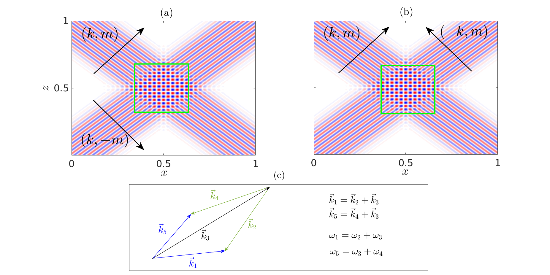
Figure 1: Examples of different orientations of propagating parent waves: in (a) vertically and (b) horizontally opposite directions, with the intersection region marked in green. (c) Frequency and wavevector triad conditions that are satisfied between the 5 waves that are involved in the interaction region. Waves 1 and 5 are parent waves, while waves 2,3, and 4 are daughter waves, with wave-3 being the common daughter wave.

In the context of internal gravity waves, 5-wave systems have been studied recently (Pan et al., 2021a, b). Pan et al. (2021a) focus on 5-wave systems where the same parent wave generates four different daughter waves, which is not the focus of this paper. Pan et al. (2021b) explore 5-wave interactions that consist of two parent waves and three daughter waves, but their focus is on rogue wave generation. They study the 5-wave systems in a 2D setting without the rotational effects. Moreover, no detailed study was conducted on the growth rates. In this paper, we consider a 3D setting with rotational effects, which is observed to be important in our case. The primary focus is on the growth rates of the daughter waves and to understand scenarios in which the 5-wave system instability is faster than the 3-wave system instability (standard triads). In our study, the frequencies of the two parent waves are always assumed to be the same, and this assumption can be important in an oceanographic context since internal waves generated by the same tide have the same frequency. The paper is organized as follows. In §2, we use multiple scale analysis to simplify the 3D, Boussinesq Navier-Stokes equations in the $f-$plane and derive the wave amplitude equations. Expressions for growth rates are provided. In §3, theoretical comparisons between the growth rates of 3-wave systems and 5-wave systems for different combinations of parent waves are provided. In §4, numerical validations are provided for the 5-wave systems, and specific focus is also given to the fate of the parent waves near the critical latitude. The paper is summarized in §5.

2 Governing equations

The 3D, incompressible, Boussinesq, Navier-Stokes equations in the $f-$plane in primitive variables are given by

$$\frac{\textnormal{D}\textbf{u}}{\textnormal{D}t}+f\hat{z}\times\textbf{u} =-\frac{1}{\rho_{0}}\nabla p+b\hat{z}+\nu\Delta\textbf{u},$$ (1a)

$$\frac{\textnormal{D}b}{\textnormal{D}t}+N^{2}w =\kappa\Delta b,$$ (1b)

$$\nabla.\textbf{u} =0.$$ (1c)

Here $\textbf{u}=(u,v,w)$, where the components respectively denote the zonal, meridional, and vertical velocities. Moreover, $f$ is the local Coriolis frequency, $\rho_{0}\approx 1000\,\textnormal{kg}\,\textnormal{m}^{-3}$ is the reference density, $p$ is the perturbation pressure, $b$ is the buoyancy perturbation, $\nu$ is the kinematic viscosity, $N$ is the background buoyancy frequency, and $\kappa$ is the diffusion coefficient. The operator $\Delta$ is defined as $\Delta\equiv\partial^{2}/\partial x^{2}+\partial^{2}/\partial y^{2}+\partial^{2}/\partial z^{2}$, while ${\textnormal{D}}/{\textnormal{D}t}$ is the material derivative.

We intend to study wave-wave interactions using multiple-scale analysis. To this end, we combine equations (1a)–(1c) into a single equation. After some simple manipulations, the single equation describing the evolution of vertical velocity is written in a compact form:

$$\frac{\partial^{2}}{\partial t^{2}}(\Delta w)+N^{2}(\nabla^{2}_{h}w)+f^{2}\frac{\partial^{2}w}{\partial z^{2}}+\textnormal{NLT}\hskip 11.38092pt=\hskip 11.38092pt\textnormal{VT},$$ (2)

where $\nabla_{h}^{2}\equiv\partial^{2}/\partial x^{2}+\partial^{2}/\partial y^{2}$. NLT denotes all the nonlinear terms:

NLT $$=\nabla^{2}_{h}\frac{\partial(\textbf{u}.\nabla w)}{\partial t}+\nabla^{2}_{h}(\textbf{u}.\nabla b)-\frac{\partial^{3}(\textbf{u}.\nabla u)}{\partial x\partial z\partial t}$$

$$+f\frac{\partial^{2}(\textbf{u}.\nabla u)}{\partial y\partial z}-f\frac{\partial^{2}(\textbf{u}.\nabla v)}{\partial x\partial z}-\frac{\partial^{3}(\textbf{u}.\nabla v)}{\partial y\partial z\partial t}.$$ (3)

Moreover, VT denotes viscous and molecular diffusion terms:

$$\textnormal{VT}=\nu\frac{\partial}{\partial t}\left(\Delta^{2}w\right)+\nabla^{2}_{h}(\kappa\Delta b)+f\nu\frac{\partial^{2}(\Delta u)}{\partial y\partial z}-f\nu\frac{\partial^{2}(\Delta v)}{\partial x\partial z}.$$ (4)

For simplicity, we assume $\kappa=0$. Furthermore, we mainly focus on plane waves. Similar to the procedure used in Bourget et al. (2013), the vertical velocity of the $j-$th wave $(j=1,2,\ldots,5)$ is assumed to be a product of a rapidly varying phase and an amplitude that slowly varies in time. Mathematically this can be written as

$$w_{j}(x,y,z,t)=a_{j}(\epsilon_{t}t)\exp{[\textnormal{i}(k_{j}x+l_{j}y+m_{j}z-\omega_{j}t)]}+\mathrm{c.c}.,$$ (5)

where $k_{j},l_{j},m_{j},$ and $\omega_{j}$ are respectively the zonal wavenumber, meridional wavenumber, vertical wavenumber, and frequency of the $j-$internal wave. ‘c.c.’ denotes the complex conjugate. The amplitude is assumed to evolve on a slow time scale $\epsilon_{t}t$, where $\epsilon_{t}$ is a small parameter. Moreover, $a_{j}$ itself is $\mathcal{O}(\epsilon_{a})$, where $\epsilon_{a}\ll 1$. For weakly nonlinear wave-wave interactions, wave steepness should be a small quantity (Koudella & Staquet, 2006), and $\epsilon_{a}$ is chosen accordingly. On substituting (5) in (2), at the leading order ($\mathcal{O}(\epsilon_{a})$) we obtain the dispersion relation in 3D:

$$\omega_{j}^{2}=\frac{N^{2}(k_{j}^{2}+l_{j}^{2})+f^{2}m_{j}^{2}}{k_{j}^{2}+l_{j}^{2}+m_{j}^{2}}.$$ (6)

All 5 waves involved in the interaction must satisfy this dispersion relation.

Energy transfer between the waves due to weakly nonlinear wave-wave interactions occurs at $\mathcal{O}(\epsilon_{a}^{2})$. For the $j$-th wave, the amplitude evolution equation reads

$$\mathcal{D}_{j}\frac{\partial a_{j}}{\partial t} =-\textnormal{NLT}_{j}+\textnormal{VT}_{j},$$ (7)

where $\mathcal{D}_{j}\equiv 2\textnormal{i}\omega_{j}(k_{j}^{2}+l_{j}^{2}+m_{j}^{2})$ is defined for convenience. $\textnormal{NLT}_{j}$ and $\textnormal{VT}_{j}$ represent all the nonlinear and viscous terms with the phase of the $j-$th wave, respectively. The expression for $\textnormal{VT}_{j}$ is given by

$$\textnormal{VT}_{j}=-\mathcal{D}_{j}{\nu}/{2}\left(\frac{f^{2}m_{j}^{2}}{\omega_{j}^{2}}+m_{j}^{2}+l_{j}^{2}+k_{j}^{2}\right).$$ (8)

$\textnormal{NLT}_{j}$ is obtained by substituting the fields $(u_{j},v_{j},w_{j},b_{j})$ in NLT, and by retaining all the nonlinear terms that have the same phase as the $j-$th wave. Nonlinear terms that do not have the phase of any of the five waves are the ‘non-resonant terms’ and are neglected. From $w_{j}$, we can obtain $u_{j},v_{j},$ and $b_{j}$ by using the polarisation relations:

$$\begin{bmatrix}u_{j}\\ \\ v_{j}\\ \\ b_{j}\end{bmatrix}=\begin{bmatrix}U_{j}\\ \\ V_{j}\\ \\ B_{j}\end{bmatrix}w_{j}=\begin{bmatrix}-{m_{j}(\omega_{j}k_{j}+\textnormal{i}l_{j}f_{j})}{/[\omega_{j}(k_{j}^{2}+l_{j}^{2})]}\\ \\ -{m_{j}(\omega_{j}l_{j}-\textnormal{i}k_{j}f_{j})}{/[\omega_{j}(k_{j}^{2}+l_{j}^{2})]}\\ \\ -\textnormal{i}{N^{2}}{/\omega_{j}}\end{bmatrix}w_{j}.$$ (9)

Polarisation expressions are also used to evaluate $\textnormal{NLT}_{j}$, the expressions for which are given in appendix A.

2.1 Wave-amplitude equations and growth rates

The amplitude evolution of each of the $5$ waves can be obtained from (7):

$$\frac{da_{1}}{dt}={\mathcal{M}}_{1}a_{2}a_{3}-\mathcal{V}_{1}a_{1},\hskip 28.45274pt\frac{da_{2}}{dt}={\mathcal{M}}_{2}a_{1}\bar{a}_{3}-\mathcal{V}_{2}a_{2}$$ (10)

$$\frac{da_{5}}{dt}=\mathcal{N}_{5}a_{4}a_{3}-\mathcal{V}_{5}a_{5}\hskip 28.45274pt\frac{da_{4}}{dt}=\mathcal{N}_{4}a_{5}\bar{a}_{3}-\mathcal{V}_{4}a_{4}$$ (11)

$$\frac{da_{3}}{dt}={\mathcal{M}}_{3}a_{1}\bar{a}_{2}+\mathcal{N}_{3}a_{5}\bar{a}_{4}-\mathcal{V}_{3}a_{3}$$ (12)

where $\mathcal{V}_{j}={\nu}/{2}\left({f^{2}m_{j}^{2}}/{\omega_{j}^{2}}+m_{j}^{2}+l_{j}^{2}+k_{j}^{2}\right)$. As depicted in figure 1(c), wave-1,-2, and -3 form a triad, whose nonlinear coefficients are given by $\mathcal{M}_{j}$. Likewise, wave-3, -4, and -5 also form a triad, whose nonlinear coefficients are given by $\mathcal{N}_{j}$. Expressions for $\mathcal{M}_{j}$ and $\mathcal{N}_{j}$ are given in appendix A. Wave-3, therefore, becomes the common daughter wave in two different triads. Moreover, wave-3 can be thought of as the daughter wave in a triad with wave-1 and -5 as the two parent waves.

Using pump wave approximation (McEwan & Plumb, 1977; Young et al., 2008), (10)–(12) can be simplified to a set of linear differential equations which are given below in a compact form:

$$\begin{bmatrix}\dfrac{d\bar{a}_{2}}{dt}\\ \\ \dfrac{d\bar{a}_{4}}{dt}\\ \\ \dfrac{d{a}_{3}}{dt}\end{bmatrix}=\begin{bmatrix}-\mathcal{V}_{2}&0&\bar{{\mathcal{M}}}_{2}\bar{A}_{1}\\ \\ \\ 0&-\mathcal{V}_{4}&\bar{\mathcal{N}}_{4}\bar{A}_{5}\\ \\ \\ {\mathcal{M}}_{3}{A}_{1}&{\mathcal{N}}_{3}{A}_{5}&-\mathcal{V}_{3}\end{bmatrix}\begin{bmatrix}\bar{a}_{2}\\ \\ \\ \bar{a}_{4}\\ \\ \\ {a}_{3}\end{bmatrix}.$$ (13)

Note that $a_{1}(a_{5})$ has been changed to $A_{1}(A_{5})$ to denote the fact that they are now constants. By assuming $da_{j}/dt=\sigma a_{j}$, we arrive at the equation

$$(\sigma+\mathcal{V}_{2})(\sigma+\mathcal{V}_{3})(\sigma+\mathcal{V}_{4})-\bar{\mathcal{N}}_{4}{\mathcal{N}}_{3}|A_{5}|^{2}(\sigma+\mathcal{V}_{2})-\bar{\mathcal{M}}_{2}{\mathcal{M}}_{3}|A_{1}|^{2}(\sigma+\mathcal{V}_{4})=0,$$ (14)

where $\sigma$ is the growth rate of the system of equations given in (13). A real, positive $\sigma$ implies the daughter waves can extract energy from the parent wave. For $\nu=0$ (inviscid flow), the growth rate has a simple expression given by

$$\sigma=\sqrt{\bar{\mathcal{M}}_{2}{\mathcal{M}}_{3}|A_{1}|^{2}+\bar{\mathcal{N}}_{4}{\mathcal{N}}_{3}|A_{5}|^{2}}.$$ (15)

Note that by setting either $A_{1}=0$ or $A_{5}=0$, we arrive at the standard growth expression for triads (3-wave systems). Moreover, we can also obtain the condition

$$\sqrt{\bar{\mathcal{M}}_{2}{\mathcal{M}}_{3}|A_{1}|^{2}+\bar{\mathcal{N}}_{4}{\mathcal{N}}_{3}|A_{5}|^{2}}\leq\sqrt{2}\widehat{\sigma}_{1}\hskip 14.22636pt\textnormal{or}\hskip 14.22636pt\sqrt{\bar{\mathcal{M}}_{2}{\mathcal{M}}_{3}|A_{1}|^{2}+\bar{\mathcal{N}}_{4}{\mathcal{N}}_{3}|A_{5}|^{2}}\leq\sqrt{2}\widehat{\sigma}_{5}$$ (16)

where $\widehat{\sigma}_{1}(\widehat{\sigma}_{5})$ is the maximum growth rate of all 3-wave systems of parent wave-1(5). If both the parent waves have the same amplitude $(A_{1}=A_{5})$, frequency, and wavevector norm, then $\widehat{\sigma}_{1}=\widehat{\sigma}_{5}$. In such cases, (16) implies that any 5-wave system’s growth rate could, in principle, be higher (maximum being $\sqrt{2}$ times) than the maximum growth rate of all 3-wave systems. For all the parent wave combinations considered in this paper, $A_{1}=A_{5}$ is consistently taken for the analysis.

2.2 5-wave system identification

For a resonant 5-wave system, all three daughter waves should satisfy the dispersion relation. This leads to 3 constraints, which are given below:

$$\omega_{3}^{2} =\frac{N^{2}(k_{3}^{2}+l_{3}^{2})+f^{2}m_{3}^{2}}{k_{3}^{2}+l_{3}^{2}+m_{3}^{2}},$$ (17a)

$$\omega_{2}^{2} =\frac{N^{2}(k_{2}^{2}+l_{2}^{2})+f^{2}m_{2}^{2}}{k_{2}^{2}+l_{2}^{2}+m_{2}^{2}},$$ (17b)

$$\omega_{4}^{2} =\frac{N^{2}(k_{4}^{2}+l_{4}^{2})+f^{2}m_{4}^{2}}{k_{4}^{2}+l_{4}^{2}+m_{4}^{2}}.$$ (17c)

The following triad conditions also add additional constraints:

$$\omega_{2} =\omega_{1}-\omega_{3},\hskip 8.5359pt\textbf{k}_{2}=\textbf{k}_{1}-\textbf{k}_{3},$$ (18a)

$$\omega_{4} =\omega_{5}-\omega_{3},\hskip 8.5359pt\textbf{k}_{4}=\textbf{k}_{5}-\textbf{k}_{3},$$ (18b)

where $\textbf{k}_{j}=(k_{j},l_{j},m_{j})$ is the wavevector of the $j-$wave. Substitution of (18a) in (17b), and (18b) in (17c) lead to

$$\omega_{3}^{2} =\frac{N^{2}(k_{3}^{2}+l_{3}^{2})+f^{2}m_{3}^{2}}{k_{3}^{2}+l_{3}^{2}+m_{3}^{2}},$$ (19a)

$$(\omega_{1}-\omega_{3})^{2} =\frac{N^{2}((k_{1}-k_{3})^{2}+(l_{1}-l_{3})^{2})+f^{2}(m_{1}-m_{3})^{2}}{(k_{1}-k_{3})^{2}+(l_{1}-l_{3})^{2}+(m_{1}-m_{3})^{2}},$$ (19b)

$$(\omega_{5}-\omega_{3})^{2} =\frac{N^{2}((k_{5}-k_{3})^{2}+(l_{5}-l_{3})^{2})+f^{2}(m_{5}-m_{3})^{2}}{(k_{5}-k_{3})^{2}+(l_{5}-l_{3})^{2}+(m_{5}-m_{3})^{2}}.$$ (19c)

Solutions for (19a)-(19c) would provide resonant 5-wave systems, and they are found by varying $(\omega_{3},k_{3},l_{3},m_{3})$. Hereafter we always assume $|\textbf{k}_{1}|=|\textbf{k}_{5}|$, however, $\textbf{k}_{1}\neq\textbf{k}_{5}$, and $\omega_{1}=\omega_{5}=0.1N$. Such small frequency values appear in many other studies, for example, Nikurashin & Legg (2011); Mathur et al. (2014).

3 Results from the reduced–order model

3.1 Parent waves in the same vertical plane

3.1.1 $\mathbf{k}_{1}=(k_{1},0,m_{1})$ and $\mathbf{k}_{5}=(k_{1},0,-m_{1})$

We first consider the scenario where the two parent waves have the same horizontal wavevector ($k,l$) but travel in vertically opposite directions, see figure 1(a). For simplicity, the meridional wavenumbers of the parent waves ($l_{1}$ and $l_{5}$) are assumed to be 0. Internal waves propagating in vertically opposite directions are ubiquitous in the oceans. For example, internal wave beams getting reflected from the bottom surface of the ocean, or from the air-water interface, or even from the pycnocline, will result in scenarios where parent waves travelling in vertically opposite directions meet.

For the given set of parent waves, a resonant 5-wave system is possible only when $\omega_{3}\approxeq\omega_{1}-f$. No other resonant 5-wave systems were found for $0<f/\omega_{1}<0.5$. Hence, the 5-wave system always consists of (a) two parent waves, each with frequency $\omega_{1}$ (as per our assumption), (b) a common daughter wave with frequency $\omega_{1}-f$, and (c) two inertial (frequency $f$) daughter waves, which also propagate in vertically opposite directions.

Next we study the growth rates of the 5-wave system. First, we decide on the viscosity values in a non-dimensionalised form. In this regard we choose $|A_{1}|/k_{1}\nu=10^{4}$ and $|A_{1}|/k_{1}\nu=10^{7}$, which are used throughout the paper. At $|A_{1}|/k_{1}\nu=10^{7}$, viscous effects are usually negligible, hence $|A_{1}|/k_{1}\nu=10^{4}$ is also considered to see what 5-wave systems are affected by the viscosity. We note in passing that $|A_{1}|/k_{1}\nu\sim\mathcal{O}(10^{6})$ was used by Bourget et al. (2013) to study triads with realistic oceanic parameters.

Figure 2(a) shows how the maximum growth rate of the 5-wave system and 3-wave systems vary with $f/\omega_{1}$ for different $\nu$. The growth rates are evaluated by fixing $k_{1}$ and $A_{1}$ as $f$ is varied. Figures 2(b)–2(c) respectively show the horizontal and the vertical wavenumbers of the daughter waves involved in the 5-wave interaction. Note that the common daughter wave’s horizontal wavevector $(k_{1},0)$ is always the same as that of the parent waves. This is expected since the other two daughter waves are inertial waves. Moreover, the common daughter wave can have a positive or negative vertical wavenumber, and both cases have the same growth rate. For low $f$ values, the 3-wave system has a higher growth rate, hence it is the dominant instability. This is because the two 3-wave systems that combine to form the 5-wave system always contain inertial daughter waves. Moreover, the growth rate of 3-wave systems containing inertial waves is much smaller than the maximum possible growth rate (Richet et al., 2018, figure 8). As a result, the resonant 5-wave system is of little significance at low latitudes.

As $f$ is increased, the 5-wave system’s growth rate becomes higher than the maximum growth rate of all 3-wave systems. The transition occurs near $f/\omega_{1}\approx 0.3$, see figure 2(a). For high values of $f/\omega_{1}$, 5-wave systems may be faster in locations where an internal wave beam gets reflected from a flat bottom surface or from a nearly flat air-water surface. However, for inclined reflecting surfaces, the results presented here (which are based on the assumption that the two parent waves have the same wavevector norm) may not be valid since inclination results in a significant change in wavevector norm (Phillips, 1977).

Finally, we note that the parent waves combination considered in this subsection produces a field that resembles an internal wave mode in a vertically bounded domain. Hence, the predictions made in this section should also hold for modes in a bounded domain. However, in a vertically bounded domain, only a discrete set of vertical wavenumbers are allowed for a particular frequency. As a result, for a resonant 5-wave system to exist, the vertical wavenumbers of the daughter waves should be a part of the discrete vertical wavenumber spectrum.

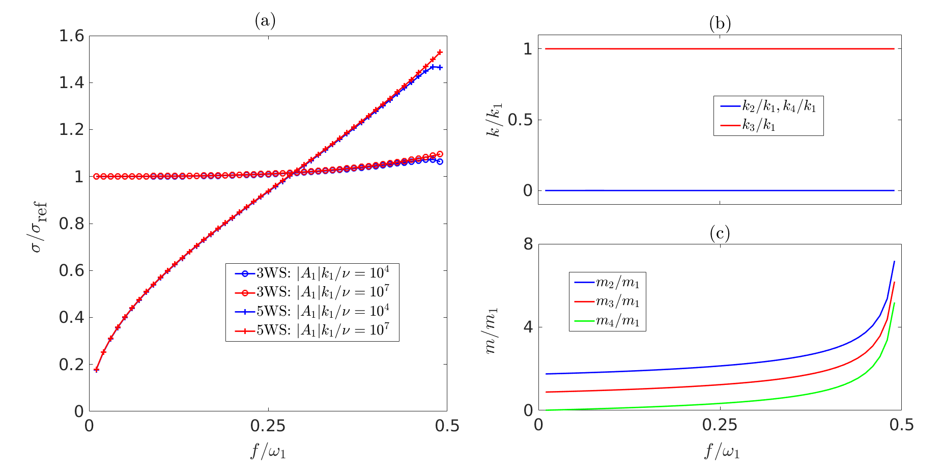
Figure 2: (a) Variation of 5-wave system’s (denoted by 5WS) growth rate and 3-wave systems’ (denoted by 3WS) maximum growth rate with $f$ for $\mathbf{k}_{1}=(k_{1},0,m_{1})$ and $\mathbf{k}_{5}=(k_{1},0,-m_{1})$ for two different viscosity values. $\sigma_{\textnormal{ref}}$ is the maximum growth rate of a 3-wave system at $f/\omega_{1}=0.01$ and $|A_{1}|/k_{1}\nu=10^{4}$. The horizontal and vertical wavenumbers of the daughter waves in the 5-wave system are respectively shown in (b) and (c). Note that in (b), $k_{2}=k_{4}=0$.

3.1.2 $\mathbf{k}_{1}=(k_{1},0,m_{1})$ and $\mathbf{k}_{5}=(-k_{1},0,m_{1})$

Here we focus on the scenario where the two parent waves have the same vertical wavenumber but travel in horizontally opposite directions, as given in figure 1(b). Moreover, $l_{1}=l_{5}=0$ is again assumed. For this particular combination of parent wavevectors, resonant 5-wave systems are possible for $\omega_{3}\in(f,0.53\omega_{1})$. For $f/\omega_{1}=0.01$, resonant 5-wave systems exist up to $\omega_{3}\approx 0.53\omega_{1}$. As $f$ increases, the maximum possible value of $\omega_{3}$ slowly reduces to $0.5\omega_{1}$. We define two branches: 5-wave systems where the common daughter wave has a positive (negative) vertical wave number is defined as Branch-1(2). Figures 3(a)–3(b) show how the maximum growth rate for each of these two branches varies with $f$ for two different viscosity values. The maximum growth rate of 3-wave systems is once again plotted so as to provide a clear comparison between 5-wave and 3-wave systems. For lower $f$ values, resonant 5-wave systems have a lesser maximum growth rate than the maximum growth rate of 3-wave systems ($\sigma/\sigma_{\textnormal{ref}}<1$). However, the 5-wave instability is faster than the 3-wave instability for the higher $f$ values. The transition once again occurs near $f\approx 0.3\omega_{1}$. All these observations are similar to that in figure 2(a). For high $f$ values, the maximum growth rate of both branches is almost the same. Viscosity has a non-negligible effect only when $f\approx\omega_{1}/2$, where the daughter waves have a high vertical wavenumber.

Figures 4(a)–4(c) show how the growth rate of both the branches vary with $\omega_{3}/\omega_{1}$ for three different $f/\omega_{1}$ values that are greater than $0.3$. Figure 4 reveals that growth rates always decrease as $\omega_{3}$ is increased, indicating the maximum growth rate is at $\omega_{3}=f$. For $f/\omega_{1}>0.3$, the common daughter wave is always an inertial wave in the most unstable 5-wave system. Interestingly, as $\omega_{3}$ is increased from $f$, the meridional wavenumber of the common daughter wave increases, hence making the instability 3D. Moreover, for the three $f$ values analysed in figure 4, the zonal wavenumber of the common daughter wave $(k_{3})$ is nearly zero for all the 5-wave systems. Note that the maximum growth rate occurs at $\omega_{3}\approx f$ where $(k_{3},l_{3})\xrightarrow{}0$. As a result, the system’s most unstable mode can be studied/simulated by considering a 2D system. The effects of viscosity are more apparent for $|A_{1}|/k_{1}\nu=10^{4}$ as expected, and Branch-1 is affected by viscous effects more than Branch-2.

For high $f$ values, inertial waves have been observed to be the daughter waves of a parent internal wave with semidiurnal frequency, see Yi et al. (2017); Richet et al. (2017, 2018); Chen et al. (2019). In topographic generation of internal waves, internal wave beams intersecting each other is quite common. The locations where internal wave beams intersect can serve as spots where a single inertial wave can extract energy from two different internal wave beams.

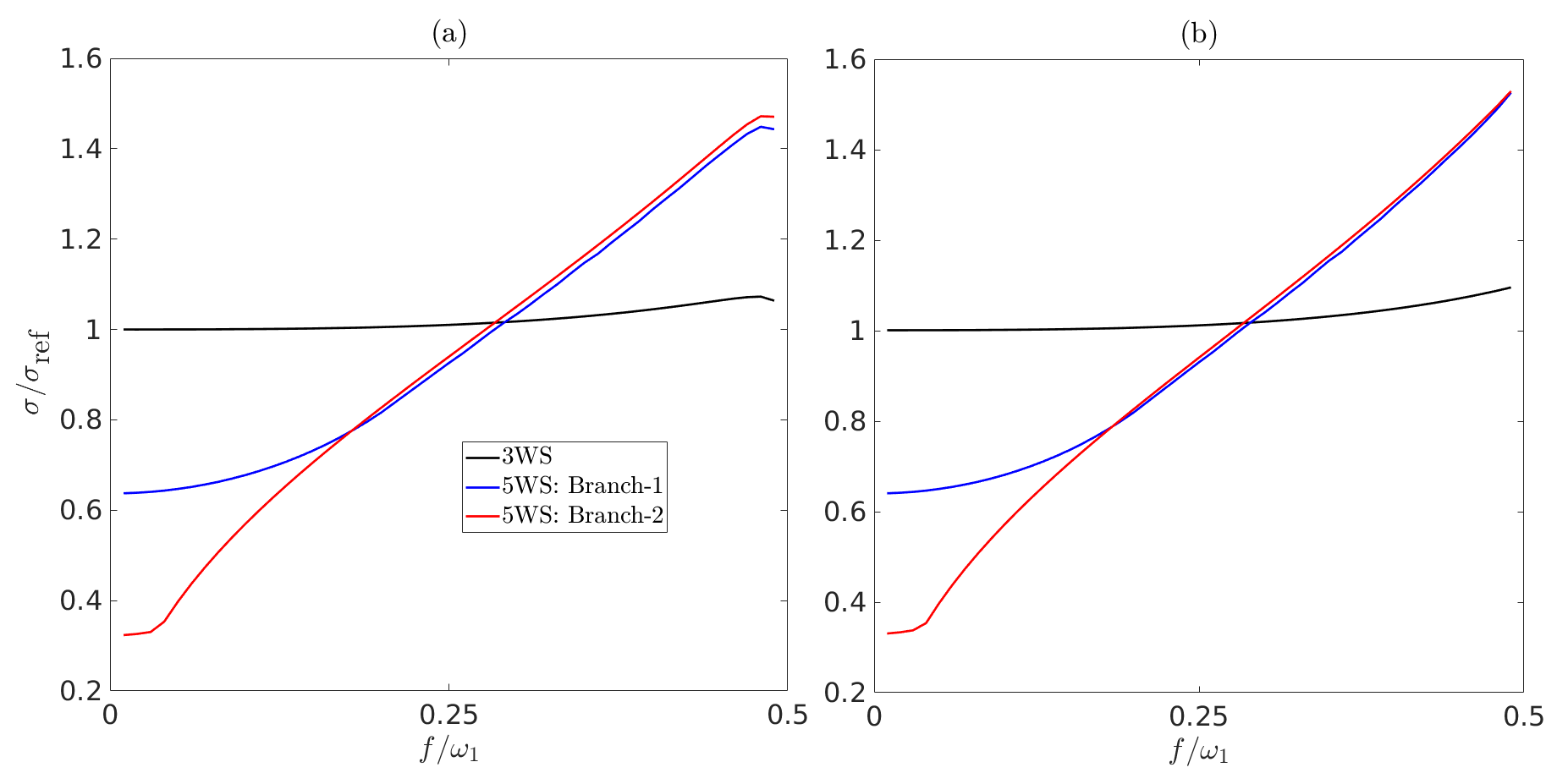
Figure 3: Comparison of maximum growth rates of 5-wave systems and 3-wave systems for $\mathbf{k}_{1}=(k_{1},0,m_{1})$ and $\mathbf{k}_{5}=(-k_{1},0,m_{1})$. (a) $|A_{1}|/k_{1}\nu=10^{4}$, and (b) $|A_{1}|/k_{1}\nu=10^{7}$.

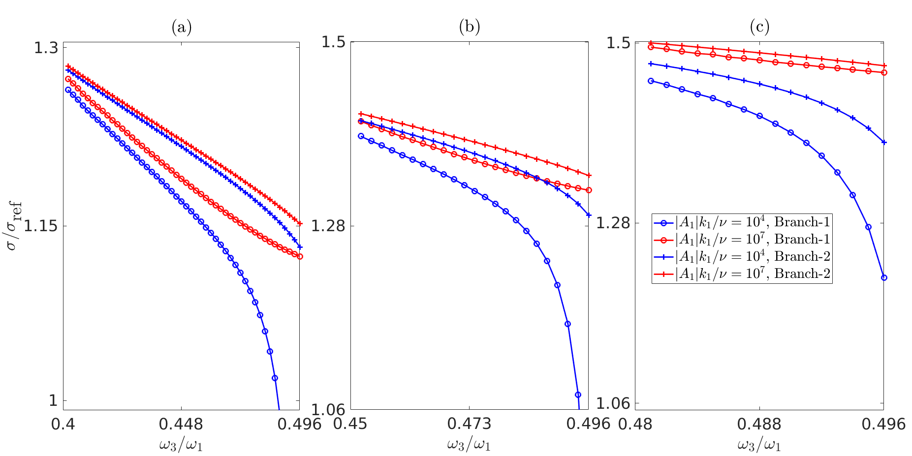
Figure 4: Growth rate variation with $\omega_{3}/\omega_{1}$ for Branch-1 and 2 for (a) $f/\omega_{1}=0.40$, (b) $f/\omega_{1}=0.45$, and (c) $f/\omega_{1}=0.48$.

3.2 Oblique parent waves

In the oceans, parent waves that are not on the same vertical plane can also propagate amidst each other. Here we study the maximum growth rate for 5-wave systems where the parent waves have a non-zero meridional wavenumber. The parent wavevectors are given by

$$\mathbf{k}_{1}=(k_{1}\sin{(\theta/2)},k_{1}\cos{(\theta/2)},m_{1}),\hskip 28.45274pt\mathbf{k}_{5}=(-k_{1}\sin{(\theta/2)},k_{1}\cos{(\theta/2)},m_{1}),$$ (20)

where the parameter $\theta$ is used to vary the angle between the two parent wavevectors in the $(k,l)$ plane. Note that $\theta=\pi$ leads to the wavevector combination $\mathbf{k}_{1}=(k_{1},0,m_{1})$ and $\mathbf{k}_{5}=(-k_{1},0,m_{1})$ considered in §3.1.2. Following (20), the condition $|\mathbf{k}_{1}|=|\mathbf{k}_{5}|$ will be automatically satisfied. The direction of the parent wavevectors can be changed by varying $\theta$, and how that impacts the growth rates of 5-wave systems will be explored and analysed. Figures 5(a)–5(c) show the variation of the maximum growth rate of 3-wave systems and 5-wave systems with $f$ respectively for three different $\theta$ values: $\pi/4$, $\pi/2$, and $3\pi/4$. Increasing $\theta$ results in 5-wave systems being less effective than 3-wave systems in the lower latitudes. For $\theta=\pi/4$, the 5-wave system is the dominant instability regardless of the latitude. A similar result is observed for $\theta=\pi/2$, however, the difference between the 5-wave and 3-wave systems is clearly reduced compared to $\theta=\pi/4$. For $\theta=3\pi/4$, the 5-wave system is the dominant instability only for $f/\omega_{1}\gtrapprox 0.25$. Note that regardless of the $\theta$ value, 5-wave instability is expected to be faster than the 3-wave instability when $f/\omega_{1}\gtrapprox 0.3$ considering the results from §3.1.2. For $\theta=\pi$ and $f/\omega_{1}\gtrapprox 0.3$, the maximum growth rate for 5-wave systems occurs when $\omega_{3}=f$. However, for $\theta=\pi/4$ and $\pi/2$, in the most unstable 5-wave system, wave-3 is not an inertial wave even for $f/\omega_{1}=0.45$. Hence, as $\theta$ is reduced, it is not necessary that the most unstable 5-wave system contains inertial waves. Note that the predictions for the 5-wave system will fail as $\theta\xrightarrow{}0$ since both parent waves will have the same wavevector.

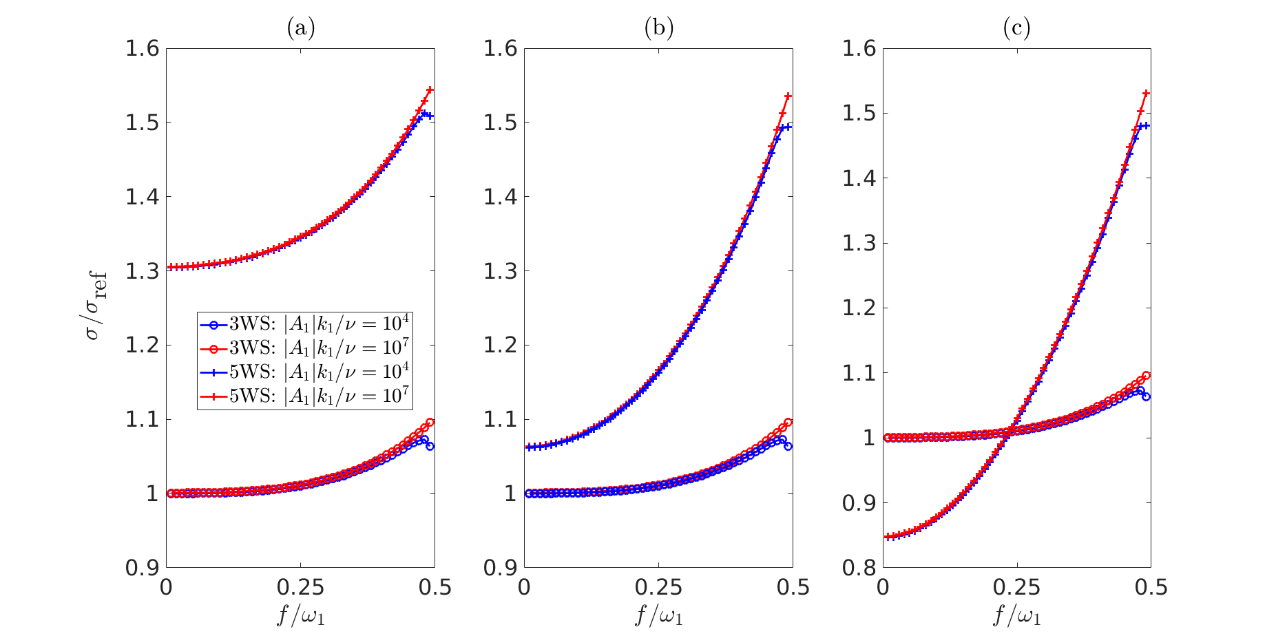
Figure 5: Variation of maximum growth rate with $f$ for 5-wave systems and 3-wave systems for a oblique set of parent waves. (a) $\theta=\pi/4$, (b) $\theta=\pi/2$, and (c) $\theta=3\pi/4$.

4 Numerical simulations

Here we present results from numerical simulations conducted to validate the predictions from reduced-order analysis presented in §3, with the primary focus being on §3.1.1 and §3.1.2. Equations (1a)–(1c) are solved with an open source pseudo-spectral code Dedalus (Burns et al., 2020). For numerical validations, we only consider 2D situations, i.e. $\partial/\partial y=0$, implying $l_{j}=0$. The details of the simulations are as follows: we fix the parent waves’ horizontal wavenumber at $k_{1}=1/H$, where $H=500$m. We consistently use $N=10^{-3}\textnormal{s}^{-1}$ and $\omega_{1}/N=0.1$. However $f/\omega_{1}$ is varied, and hence the vertical wavenumber of the parent waves ($m_{1}$) is a function of $f/\omega_{1}$. The amplitude of the parent waves is chosen such that the maximum zonal velocity ($u$) is always $0.001\textnormal{ms}^{-1}$. Computational time is variable and depends on the simulation in question. For all simulations, $4$-th order Runge-Kutta method is used as the time-stepping scheme with a time step size of $(2\pi/\omega_{1})/800$ (i.e. $800$ steps for one time period of the parent wave). All the fields are expressed using Fourier modes in the horizontal direction, and either 64 or 128 modes are used per one horizontal wavelength of the parent wave. Moreover, the vertical direction is resolved using Chebyshev polynomials or Fourier modes, and the resolution is varied from a minimum of 96 to a maximum of 512 grid points per one vertical wavelength of the parent wave. All simulations are initialised with a small amplitude noise, the spectrum of which is given by

$$\mathcal{R}_{\textrm{noise}}(x,z)=\int_{0}^{k_{\textrm{noise}}}\int_{m_{\textrm{lowest}}}^{m_{\textrm{noise}}}A_{\textrm{noise}}\sin(kx+mz+\phi_{\textrm{noise}}(k,m))dmdk,$$ (21)

where $\phi_{\textrm{noise}}(k,m)\in[0,2\pi]$ is the random phase part, which is generated using the ‘rand’ function in Matlab for each $(k,m)$. Unless otherwise specified, $k_{\textrm{noise}}=48k_{1}$ and $m_{\textrm{noise}}=48m_{1}$. Moreover, $m_{\textrm{lowest}}=2\pi/Lz$, where $Lz$ is the length of the domain in the $z$-direction. Equation (21) is added to the $b$ or $v$ field. The noise amplitude $A_{\textrm{noise}}$ is at least $10^{-3}$ times smaller than the primary waves’ corresponding amplitude. Unless otherwise mentioned, $\nu=10^{-6}\textnormal{m}^{2}\textnormal{s}^{-1}$ is taken. Equation (21) is added to the $b$ or $v$ field. The noise amplitude $A_{\textrm{noise}}$ is at least $10^{-3}$ times smaller than the primary waves’ corresponding amplitude. Unless otherwise mentioned, $\nu=10^{-6}\textnormal{m}^{2}\textnormal{s}^{-1}$ is taken.

4.1 $\mathbf{k}_{1}=(k_{1},0,m_{1})$ and $\mathbf{k}_{5}=(k_{1},0,-m_{1})$

We first focus on the parent wavevector combination $\mathbf{k}_{1}=(k_{1},0,m_{1})$ and $\mathbf{k}_{5}=(k_{1},0,-m_{1})$. As mentioned previously, the combination of wavevectors $\mathbf{k}_{1}=(k_{1},0,m_{1})$ and $\mathbf{k}_{5}=(k_{1},0,-m_{1})$ leads to fields that are very similar to an internal wave mode in a vertically bounded domain. As a result, we also simulate low modes (modes-1 and 2) in a vertically bounded domain to observe whether there is an emergence of the ‘5-wave instability’. The decay of the parent waves are simulated at specific latitudes where the daughter waves’ vertical wavenumbers in the resonant 5-wave system are multiples of $m_{1}/3$ or $m_{1}/2$. This choice helps in reducing the computational resources required for the simulations. To estimate the energy in different wavevectors, we simply use the Fast Fourier Transform (FFT) for both $x$ and $z$ directions in simulations where the parent waves are plane waves. In a vertically bounded domain, FFT is used only in the $x$ direction, while for the $z-$direction, the orthogonal nature of the modes is exploited. As a measure of the energy contained in a wavevector, a non-dimensionalised energy $\widehat{E}$ is introduced:

$$\widehat{E}(k,0,m,t)=\frac{|\hat{u}(k,0,m,t)|^{2}+|\hat{w}(k,0,m,t)|^{2}+|\hat{v}(k,0,m,t)|^{2}+|\hat{b}(k,0,m,t)|^{2}/N^{2}}{E_{\textnormal{ref}}}$$ (22)

where the hat variables ($\hat{u},\hat{w},\hat{v},\hat{b}$) respectively denote the Fourier amplitudes of (${u},{w},{v},{b}$). $E_{\textnormal{ref}}$ serves as the measure of parent waves’ energy at $t=0$ and is defined as

$$E_{\textnormal{ref}}=\left(|\hat{u}(k_{1},0,m_{1})|^{2}+|\hat{w}(k_{1},0,m_{1})|^{2}+|\hat{v}(k_{1},0,m_{1})|^{2}+|\hat{b}(k_{1},0,m_{1})|^{2}/N^{2}\right)\bigg{|}_{t=0}$$ (23)

We simulate a total of 6 cases: 2 cases for parent waves in an unbounded domain (plane waves), and 2 cases each for mode-1 and mode-2 waves in a vertically bounded domain. For mode-1, $m_{\textrm{noise}}=96m_{1}$ is chosen. For every simulation, a different $f$ value is used, and hence the resonant 5-wave system is different in each case. Figure 6 shows the exponential growth of daughter waves at 6 different latitudes due to 5-wave interactions. Figures 6(a)–6(e) plot four different wavevectors. The wavevector $(|k_{1}|,0,|m_{1}|)$ contains the energy of both parent waves, while the other three wavevectors indicate the daughter waves. All three daughter waves grow exponentially, which provides clear evidence that this is a 5-wave system. In 6(f), two different 5-wave systems emerge and both of them are plotted. Note that as the $f$ value increases, the daughter waves’ vertical wavenumber also increases in the simulations (see the legend) which is in line with the theoretical predictions given in figure 2(c). In all six simulations, inertial waves are present ($k=0$). The growth rate of the daughter waves is calculated by estimating $d\ln{(\widehat{E})}/dt$. The comparison of growth rates from simulations and theory is presented in figure 7, which shows a reasonably good agreement. For all the cases, the average of the three daughter waves’ growth rate in a particular 5-wave system is taken. Moreover, figure 7 reveals that the growth rates are well above the maximum growth rate of all 3-wave systems. Note that the 5-wave interactions can happen for standing modes only at specific latitudes because the vertical wavenumbers are discrete, not continuous. However, for plane waves, there is no such constraint. As per the predictions in §3, 5-wave interactions should be faster than the 3-wave interactions provided $f/\omega_{1}\gtrapprox 0.3$.

It was observed that as $f/\omega_{1}\xrightarrow[]{}0.5$, multiple daughter wave combinations grow and extract a considerable amount of energy from the parent waves. This can even be seen in figure 6(f), where two different 5-wave systems emerge and extract a significant amount of energy. As $f/\omega_{1}\xrightarrow[]{}0.5$, multiple 5-wave systems can become coupled and grow at a rate which is faster than any single 5-wave system (discussed in detail in §4.2). Hence, the growth rates predicted from a single 5-wave interaction will not be accurate when $f\approx\omega_{1}/2$. As $f\xrightarrow[]{}\omega_{1}/2$, the growth rate for a mode-1 wave with zonal velocity amplitude $0.002\textnormal{ms}^{-1}$ will approach $2\sigma_{\textnormal{cl}}$ instead of $\sqrt{2}\sigma_{\textnormal{cl}}$, where $\sigma_{\textnormal{cl}}$ is the maximum growth rate for a plane wave with zonal velocity amplitude $0.001\textnormal{ms}^{-1}$ at the critical latitude (Young et al., 2008). We realise that in Young et al. (2008), the mode-1 wave was considered in the presence of a non-constant $N$. However, their prediction is still expected to hold in the present scenario (constant $N$). Our numerical simulations (results not shown here) also show the growth rates of the daughter waves being well above $\sqrt{2}\sigma_{\textnormal{cl}}$ for $f\approx\omega_{1}/2$.

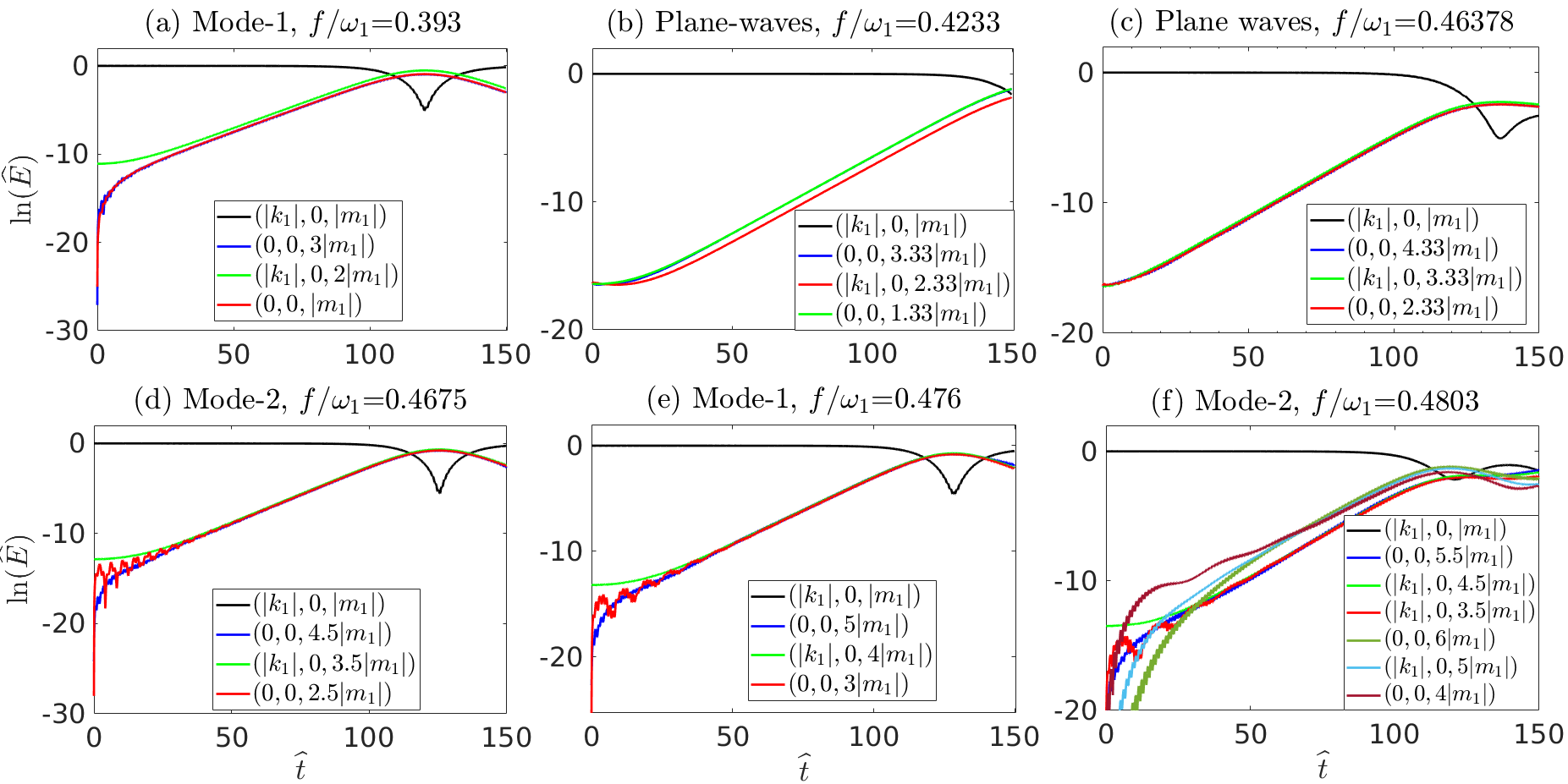
Figure 6: 5-wave interactions for plane waves, mode-1, and mode-2 different $f$ values (i.e. latitudes), plotted in ascending order. $\widehat{t}\equiv t\omega_{1}/2\pi$.

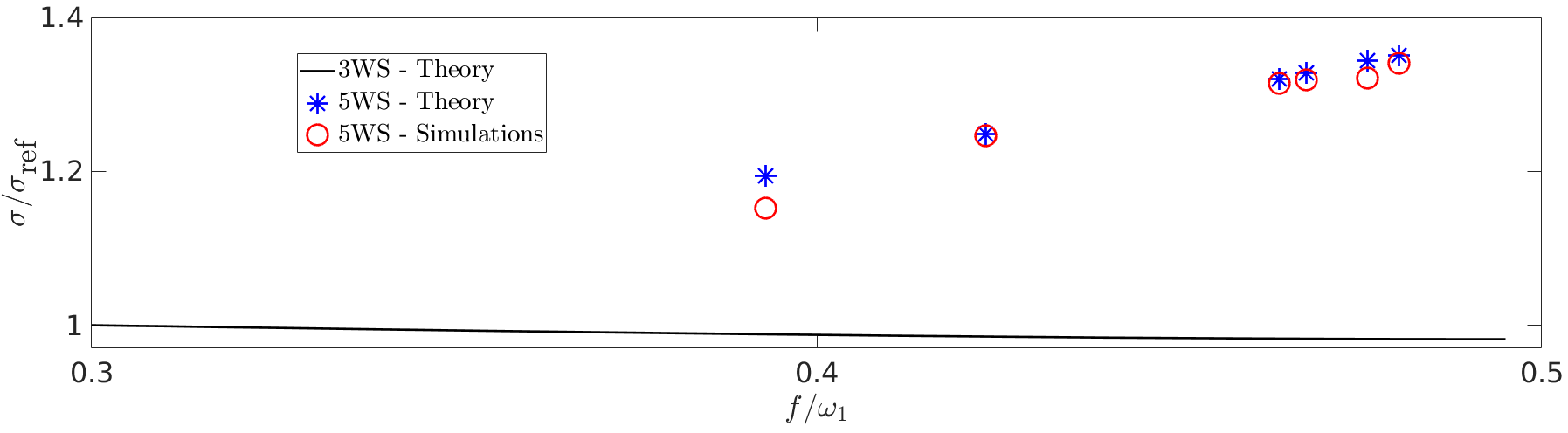
Figure 7: Comparison between theoretical growth rates and growth rates obtained from the simulations for $\mathbf{k}_{1}=(k_{1},0,m_{1})$ and $\mathbf{k}_{5}=(k_{1},0,-m_{1})$. Red (blue) markers indicate results from the simulations (theory), see legend. The black curve plots the variation of maximum growth rate of 3-wave systems with $f$.

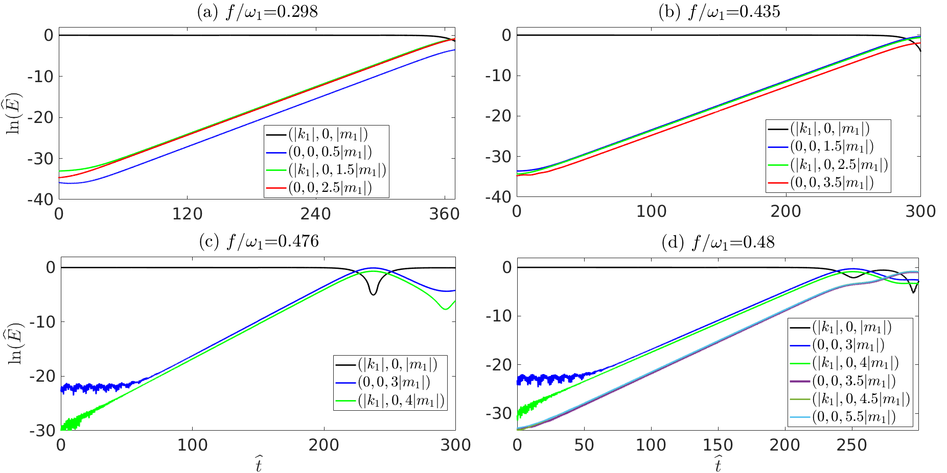
Figure 8: Four different 5-wave interactions for parent waves with wavevectors $\mathbf{k}_{1}=(k_{1},0,m_{1})$ and $\mathbf{k}_{5}=(-k_{1},0,m_{1})$.

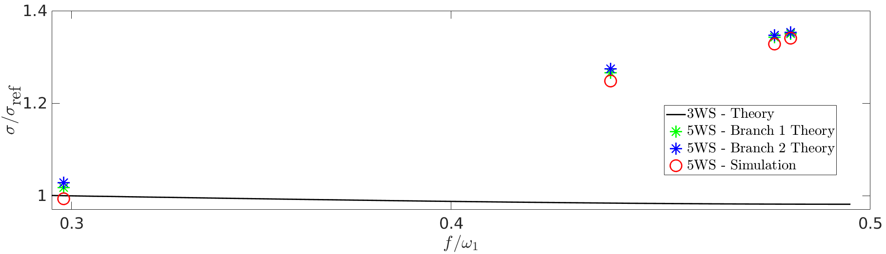
Figure 9: Comparison between theoretical growth rates and growth rates obtained from the simulations for $\mathbf{k}_{1}=(k_{1},0,m_{1})$ and $\mathbf{k}_{5}=(-k_{1},0,m_{1})$. Red markers indicate results from the simulations. Blue and green markers are predictions from the reduced order model. The black curve plots the variation of maximum growth rate of all 3-wave systems with $f$.

4.2 $\mathbf{k}_{1}=(k_{1},0,m_{1})$ and $\mathbf{k}_{5}=(-k_{1},0,m_{1})$

We now validate 5-wave interactions for parent waves propagating in horizontally opposite directions. In this regard, we focus on latitudes where the daughter waves’ vertical wavenumbers are multiples of $m_{1}/2$. Figure 8 shows the growth of daughter waves for four different $f/\omega_{1}$ values. Figures 8(a)–8(b) show energy in three wavevectors growing exponentially. The three wavevectors encompass both branch-1 and branch-2 daughter waves’ wavevectors, and the simulation results are in line with theoretical predictions. The green curve (the wave with non-zero horizontal wavenumber) contains the energy of both leftward and rightward propagating waves. The growth rates estimated from the simulations are much higher than what is expected for a 3-wave interaction. For example, at $f=0.298\omega_{1}$, the growth rate of the daughter waves is $\approx 30\%$ more than the growth rate of the individual 3-wave interactions that combine to form the 5-wave interaction. Figure 8(c) shows only two daughter waves, which are part of the Branch-2 5-wave system. In this case, Branch-1 did not have a growth comparable to Branch-2. Finally, 8(d) has three distinct 5-wave systems

• System-1 (daughter waves): $(k_{1},0,4m_{1})$, $(-k_{1},0,4m_{1})$, $(0,0,-3m_{1})$,

• System-2 (daughter waves): $(k_{1},0,4.5m_{1})$, $(-k_{1},0,4.5m_{1})$, $(0,0,-3.5m_{1})$,

• System-3 (daughter waves): $(k_{1},0,-4.5m_{1})$, $(-k_{1},0,-4.5m_{1})$, $(0,0,5.5m_{1})$.

System-1 is also present for $f/\omega_{1}=0.476$. This 5-wave system is present in both $f/\omega_{1}=0.476$ and $0.48$ because the change in $f$ is not that significant and hence the specific interaction is not expected to be detuned significantly. As a result, the system has an exponential growth. Even though the growth rates of System-2 and System-3 are observed to be higher than the growth rate of System-1, System-1 drains the largest amount of energy from the parent waves because the daughter waves in this system have a slightly higher energy at $t=0$. Growth rates obtained from the reduced order models are once again compared with the growth rates obtained from the numerical simulations, see figure 9. When there are multiple branches growing, the average growth rate of the (two) branches is taken since both branches have nearly the same growth rate. For $f/\omega_{1}=0.48$ in figure 8(d), the average of system-2 and system-3’s growth rates is compared with the theoretical growth rate since these are the two resonant Branch-1 and Branch-2 systems at $f/\omega_{1}=0.48$. It can be seen that theoretical predictions match reasonably well with the simulations. Moreover, similar to §4.1, the growth rates of 5-wave systems are well above the maximum growth of 3-wave systems (shown by the black curve in figure 9) for $f/\omega_{1}>0.4$.

4.3 Simulations and analysis for $f\approx\omega_{1}/2$

In §4.1, we saw that the theoretical growth rates of 5-wave systems are not accurate for $f\approx\omega_{1}/2$. To test whether the 5-wave systems’ growth rate holds near the critical latitude for $\mathbf{k}_{1}=(k_{1},0,m_{1})$ and $\mathbf{k}_{5}=(-k_{1},0,m_{1})$, we ran simulations for three different $f/\omega_{1}$ values: $f/\omega_{1}=0.496,0.498$ and $0.499$. Moreover, for each $f$, we ran three simulations: one with $\nu=10^{-6}\textnormal{m}^{2}\textnormal{s}^{-1}$, one with $\nu=0.25\times 10^{-6}\textnormal{m}^{2}\textnormal{s}^{-1}$, and finally one simulation with hyperviscous terms instead of viscous terms (i.e. by setting $\nu=0$). The hyperviscous operator $-\nu_{H}\Delta^{4}()$ is added to right hand side of (1a)–(1b) with $\nu_{H}=0.25\times 10^{-6}\textnormal{m}^{8}\textnormal{s}^{-1}$. Hyperviscous terms are intended to make the simulation nearly inviscid, and they have been used previously to study PSI (Hazewinkel & Winters, 2011). All simulations are run for $150$ time periods of the parent wave. The simulations are stopped before the small-scale daughter waves attain energy comparable to the parent waves. The small-scale waves will break in such cases, and the ensuing turbulence is not resolved and is also not the focus of this study. We are only interested in the growth rate of the daughter waves.

Figure 10 shows the non-dimensionalised growth rates ($\sigma/\sigma_{\textnormal{cl}}$) of the daughter waves for all nine cases. In figure 10, each row is for a different $f$ value. Moreover, for each column, $\nu$ or $\nu_{H}$ is held constant. For the hyperviscous simulations and simulations with the lower viscosity, it can be seen that the non-dimensionalised growth rates are well above $\sqrt{2}$ for all three $f$-values (second and third column of figure 10). Daughter waves with $m=20-40m_{1}$ have $\sigma/\sigma_{\textnormal{cl}}\approx 1.85$ in the simulations with hyperviscous terms. For each $f$, simulations with $\nu=10^{-6}\textnormal{m}^{2}\textnormal{s}^{-1}$ have considerably lower growth rates (especially for higher wavenumbers) compared to the other simulations because of the viscous effects.

We provide the reason for $\sigma/\sigma_{\textnormal{cl}}$ being well above $\sqrt{2}$ using the reduced order model. The dispersion relation for the daughter waves can be rewritten as

$$(f+\delta\omega)^{2}=\frac{N^{2}(nk_{1})^{2}+f^{2}m^{2}}{(nk_{1})^{2}+m^{2}},$$ (24)

where $\delta\omega$ is the difference between the wave’s frequency ($f+\delta\omega$) and the inertial frequency ($f$), and $n$ is some constant (but for our purposes, will primarily be an integer). Note that $k_{1}$ is the zonal wavenumber of the parent waves, but $m$ is not the vertical wavenumber of parent waves. Near the critical latitude, in a wave-wave interaction, any daughter wave’s frequency would be approximately equal to the inertial frequency, implying $\delta\omega\!\ll\!f$. Hence (24) leads to

$$\frac{\delta\omega}{f}\approx\frac{(N^{2}-f^{2})(nk_{1})^{2}}{2f^{2}[(nk_{1})^{2}+m^{2}]}\ll 1.$$ (25)

In scenarios where $N^{2}\gg f^{2}$, this yields

$$m^{2}\gg\frac{N^{2}(nk_{1})^{2}}{2f^{2}}.$$ (26)

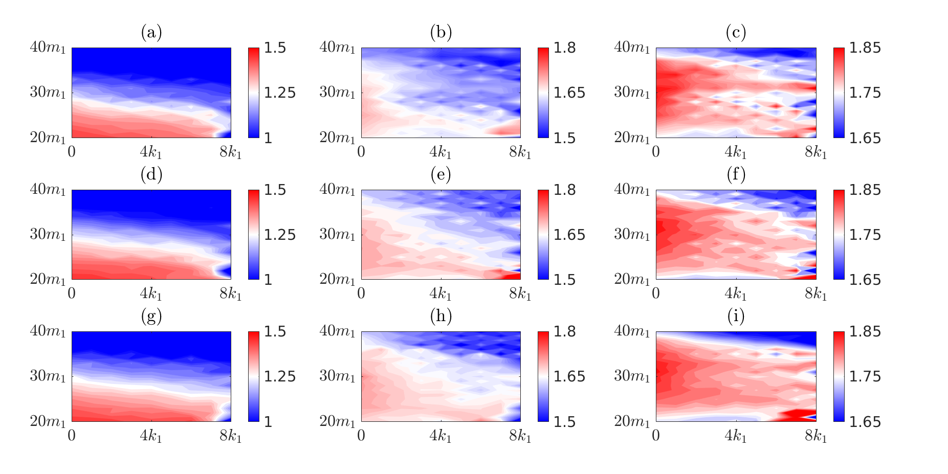
Figure 10: Growth rate contours ($\sigma/\sigma_{\textnormal{cl}}$) for the parent waves with wavevectors $\mathbf{k}_{1}=(k_{1},0,m_{1})$ and $\mathbf{k}_{5}=(-k_{1},0,m_{1})$ near the critical latitude ($f/\omega_{1}\approx 0.5$). $f/\omega_{1}=0.496$ for Row-1 ((a), (b) and (c)), $f/\omega_{1}=0.498$ for Row-2 ((d), (e) and (f)), and $f/\omega_{1}=0.499$ for Row-3 ((g), (h) and (i)). Viscosity/hyperviscosity values used are as follows: $\nu=10^{-6}\textnormal{m}^{2}\textnormal{s}^{-1}$ for Column-1 ((a), (d) and (g)), $\nu=0.25\times 10^{-6}\textnormal{m}^{2}\textnormal{s}^{-1}$ for Column-2 ((b), (e) and (h)), and $\nu_{H}=0.25\times 10^{-6}\textnormal{m}^{8}\textnormal{s}^{-1}$ for Column-3 ((c), (f) and (i)).

Near the critical latitude, $2f\approx\omega_{1}$. As a result, the sum of two daughter waves’ frequencies would be $\approx\!\omega_{1}$ provided their wavenumbers satisfy (26). As a consequence of this special scenario, a chain of coupled triads is possible as shown in figure 11. Every box contains the wavevector of a daughter wave. The absolute value of the horizontal wavenumber is lowest at the center of the chain, and it increases in either direction. However, the vertical wavenumber takes only two values. Note that $n$ would be an integer considering how the absolute value of the horizontal wavenumber increases in either direction of the central box $(0,0,m)$. Any two boxes that are connected by the same blue line add up to give a parent wave’s wavevector. For example, $(2k_{1},0,m)+(-k_{1},0,m_{1}-m)$ gives $(k_{1},0,m_{1})$, which is the wavevector of one of the parent waves. Moreover, $(-k_{1},0,m_{1}-m)+(0,0,m)$ gives $(-k_{1},0,m_{1})$, which is the other parent wave’s wavevector. Except for the daughter waves at the ends of the chain, every daughter wave would be forced by both parent waves. Assuming the wavenumbers of the daughter waves in the chain satisfy (26), the sum of any two waves’ frequencies would be $\approx\omega_{1}$, thus satisfying all the required triad conditions. For a fixed $m$, $\delta\omega$ would increase as $n$ is increased, which is evident from (24). Hence for very large $n$, the daughter wave’s frequency ($f+\delta\omega$) cannot be approximated by $f$ and the sum of two daughter waves’ frequencies cannot be approximated by $\omega_{1}$ simply because $\delta\omega$ would be large. As a result, the triad conditions would not be satisfied for very large $n$. Assuming $\delta\omega$ is negligible up to some $n$, the wave amplitude equations for the $2n+1$ daughter waves shown in figure 11 can be written in a compact way as follows:

$$\frac{d\mathbf{a}}{dt} =\mathcal{H}\mathbf{\bar{a}}$$ (27)

$$\mathbf{a} =[a_{-n}\hskip 5.69046pta_{1-n}\hskip 5.69046pt\dots\hskip 5.69046pta_{n-1}\hskip 5.69046pta_{n}]^{T}$$ (28)

$$\mathcal{H} =\begin{bmatrix}-\mathcal{V}_{-n}&\mathcal{M}_{(-n,1-n)}{A}_{1}&0&0&0\\ \mathcal{M}_{(1-n,-n)}{A}_{1}&-\mathcal{V}_{1-n}&\mathcal{N}_{(1-n,2-n)}{A}_{5}&0&0\\ \vdots&\ddots&\ddots&\ddots&\vdots\\ 0&0&\mathcal{M}_{(n-1,n-2)}{A}_{1}&-\mathcal{V}_{n-1}&\mathcal{N}_{(n-1,n)}{A}_{5}\\ 0&0&0&\mathcal{N}_{(n,n-1)}{A}_{5}&-\mathcal{V}_{n}\\ \end{bmatrix}$$ (29)

where the coefficients $\mathcal{N}_{(i,j)}$ and $\mathcal{M}_{(i,j)}$ are given by

$$\mathcal{N}_{(i,j)}=\frac{\mathfrak{N}_{(i,5,j)}}{\mathcal{D}_{i}},\hskip 14.22636pt\mathcal{M}_{(i,j)}=\frac{\mathfrak{N}_{(i,1,j)}}{\mathcal{D}_{i}}.$$ (30)

The expression for $\mathfrak{N}_{(i,*,j)}$ is given in Appendix A. Equation (27) is an extension of the system given in (13) to an arbitrary number of daughter waves. Note that using $n=1$ in (27) would result in equation (13). The growth rate for the system given in (27) can be found by calculating the eigenvalues of $\mathcal{H}$. In addition to the $\mathbf{k}_{1}=(k_{1},0,m_{1})$ and $\mathbf{k}_{5}=(-k_{1},0,m_{1})$ case, we also analyze the theoretical growth rates for oblique parent waves near the critical latitude using (27). To this end, we consider four $\theta$ values: $\theta=\pi/4$, $\pi/2$, $3\pi/4$, and $\pi$ (see (20) for the definition of $\theta$). For $\theta\neq\pi$, the parent waves have a non-zero meridional wavenumber ($l_{1}$). In such cases, the meridional wavenumber of all the daughter waves in the chain is simply assumed to be $l_{1}/2$. For all four $\theta$ values, figure 12 shows the gradual increase of the growth rate as $n$ increases for two different $m$ values. The vertical wavenumbers are chosen to be a large value so that they satisfy (26) up to $n=7$. For all the $\theta$ values, $\sigma/\sigma_{\textnormal{cl}}\approx 2$ for the higher $n$ values, which is what we observed in the simulation results shown in figure 10. Moreover, for $n=1$, $\sigma/\sigma_{\textnormal{cl}}\approx\sqrt{2}$ which is what we would expect for a 5-wave system with three daughter waves. Interestingly, for an oblique set of parent waves, the results are similar to the 2D case. Hence, 5-wave system growth rates do not apply near the critical latitude for an oblique set of parent waves as well. Note that even though high values of $m$ are used in the reduced order model, simulations show that the resonance can occur even at $m=20-40m_{1}$. As a result, near the critical latitude, regardless of the $\theta$ value, two parent waves force daughter waves as if they are a single wave with approximately twice the amplitude.

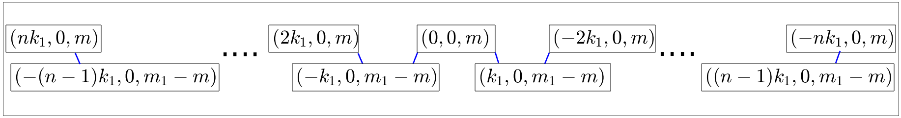
Figure 11: A simplified schematic showing how different daughter waves are coupled. Any two wavevectors (boxes) connected by the same blue line can act as a daughter wave combination for the wavevector $\textbf{k}_{1}=(k_{1},0,m_{1})$ or $\textbf{k}_{5}=(-k_{1},0,m_{1})$.

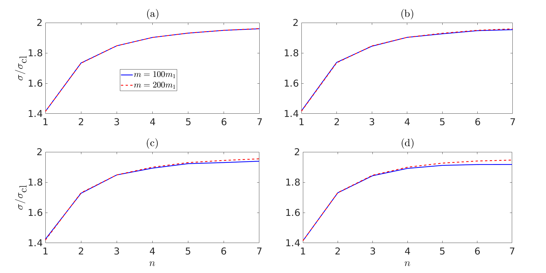
Figure 12: Variation of maximum growth rate with $n$ for triad chains near the critical latitude. (a) $\theta=\pi/4$, (b) $\theta=\pi/2$, (c) $\theta=3\pi/4$, and (d) $\theta=\pi$. Two different $m$ values are shown for each $\theta$.

5 Conclusions

Wave-wave interactions play a major role in the energy cascade of internal gravity waves. In this paper, we use multiple scale analysis to study wave-wave interactions of two plane parent waves co-existing in a region. The main instability mechanism that is focused on is the 5-wave system instability that involves two parent waves and three daughter waves. The 5-wave system is composed of two different triads (3-wave systems) with one daughter wave being a part of both triads (see figure 1(c)). For parent waves with wavevectors $(k_{1},0,m_{1})$ and $(k_{1},0,-m_{1})$, the 5-wave system is only possible when the common daughter wave’s frequency is almost equal to $\omega_{1}-f$ (where $\omega_{1}$ is the parent wave’s frequency). The other two daughter waves are inertial waves that always propagate in vertically opposite directions. The growth rate of the above-mentioned 5-wave system is higher than the maximum growth rate of 3-wave systems for $f/\omega_{1}\gtrapprox 0.3$. For parent waves with wavevectors $(k_{1},0,m_{1})$ and $(-k_{1},0,m_{1})$ (parent waves that propagate in horizontally opposite directions), similar to the previous parent wave combination, the maximum growth rate of 5-wave systems is higher than the maximum growth rate of 3-wave systems for $f/\omega_{1}\gtrapprox 0.3$. For $f/\omega_{1}\gtrapprox 0.3$, the common daughter wave’s frequency is nearly equal to $f$ in the most unstable 5-wave system. Moreover, as the common daughter wave’s frequency is increased from $f$, the meridional wavenumber increases significantly while the zonal wavenumber of the common daughter wave stays negligible.

We also study 5-wave systems for cases where the two parent waves are not confined to the same vertical plane. In such scenarios, the dominance of the 5-wave systems increase as the angle between the horizontal wavevectors of the parent waves (denoted by $\theta$) is decreased. Moreover, for any $\theta$, the 5-wave system’s instability is more dominant than the 3-wave system’s instability for $f\gtrapprox 0.3\omega_{1}$. Numerical simulations are conducted to test the theoretical predictions, and the theoretical growth rate of the 5-wave systems matches reasonably well with the results of the numerical simulations for a wide range of $f-$values. However, for all the 2D parent wave combinations considered, the growth rates from the simulations do not match the theoretical 5-wave systems’ growth rate near the critical latitude where $f\approx\omega_{1}/2$. Near the critical latitude, more than two triads become coupled, hence a chain of daughter waves is forced by the two parent waves. By modifying the reduced order model to account for a chain of daughter waves, the maximum growth rate is shown to be twice the maximum growth rate of all 3-wave systems. Moreover, the reduced order model showed similar results for parent waves that are not on the same vertical plane. Hence, near the critical latitude, the 5-wave systems’ prediction is not expected to hold for oblique parent waves as well.

Declaration of interests. The authors report no conflict of interest.

Appendix A Nonlinear coupling coefficients

The quantities $\mathfrak{N}_{(j,p,d)}$ and $\mathfrak{O}_{(j,b,c)}$ are defined so that the nonlinear coefficients can be written in a compact form:

$$\mathfrak{N}_{(j,p,d)}= -{(\omega_{p}-\omega_{d})k_{j}m_{j}}\left[\left(U_{p}\bar{U}_{d}(k_{j})+U_{p}\bar{V}_{d}l_{p}-V_{p}\bar{U}_{d}l_{d}+U_{p}m_{p}-m_{d}\bar{U}_{d}\right)\right]$$

$$-{(\omega_{p}-\omega_{d})l_{j}m_{j}}\left[\left(V_{p}\bar{V}_{d}(l_{j})-U_{p}\bar{V}_{d}k_{d}+V_{p}\bar{U}_{d}k_{p}+V_{p}m_{p}-m_{d}\bar{V}_{d}\right)\right]$$

$$+{(\omega_{p}-\omega_{d})(l_{j}^{2}+k_{j}^{2})}\left[\bar{V}_{d}l_{p}-l_{d}V_{p}+m_{j}+k_{p}\bar{U}_{d}-U_{p}k_{d}\right]$$

$$+\textnormal{i}{(l_{j}^{2}+k_{j}^{2})}\left[\bar{U}_{d}B_{p}k_{p}-U_{p}\bar{B}_{d}k_{d}+\bar{V}_{d}B_{p}l_{p}-V_{p}\bar{B}_{d}l_{d}+B_{p}m_{p}-\bar{B}_{d}m_{d}\right]$$

$$+\textnormal{i}{fl_{j}m_{j}}\left[\left(U_{p}\bar{U}_{d}(k_{j})+U_{p}\bar{V}_{d}l_{p}-V_{p}\bar{U}_{d}l_{d}+U_{p}m_{p}-m_{d}\bar{U}_{d}\right)\right]$$

$$-\textnormal{i}{fk_{j}m_{j}}\left[\left(V_{p}\bar{V}_{d}(l_{j})-U_{p}\bar{V}_{d}k_{d}+V_{p}\bar{U}_{d}k_{p}+V_{p}m_{p}-m_{d}\bar{V}_{d}\right)\right],$$ (31)

$$\mathfrak{O}_{(j,b,c)}= -{(\omega_{b}+\omega_{c})k_{j}m_{j}}\left[\left(U_{b}{U}_{c}(k_{j})+U_{b}{V}_{c}l_{b}+V_{b}{U}_{c}l_{c}+U_{b}m_{b}+{U}_{c}m_{c}\right)\right]$$

$$-{(\omega_{b}+\omega_{c})l_{j}m_{j}}\left[\left(V_{b}{V}_{c}l_{j}+U_{b}{V}_{c}k_{c}+V_{b}{U}_{c}k_{b}+V_{b}m_{b}+m_{c}{V}_{c}\right)\right]$$

$$+{(\omega_{b}+\omega_{c})(l_{j}^{2}+k_{j}^{2})}\left[{V}_{c}l_{b}+l_{c}V_{b}+m_{j}+k_{b}{U}_{c}+U_{b}k_{c}\right]$$

$$+\textnormal{i}{(l_{j}^{2}+k_{j}^{2})}\left[{U}_{c}B_{b}k_{b}+U_{b}{B}_{c}k_{c}+{V}_{c}B_{b}l_{b}+V_{b}{B}_{c}l_{c}+B_{b}m_{b}+{B}_{c}m_{c}\right]$$

$$+\textnormal{i}{fl_{j}m_{j}}\left[\left(U_{b}{U}_{c}k_{j}+U_{b}{V}_{c}l_{b}+V_{b}{U}_{c}l_{c}+U_{b}m_{b}+m_{c}{U}_{c}\right)\right]$$

$$-\textnormal{i}{fk_{j}m_{j}}\left[\left(V_{b}{V}_{c}l_{j}+U_{b}{V}_{c}k_{c}+V_{b}{U}_{c}k_{b}+V_{b}m_{b}+m_{c}{V}_{c}\right)\right],$$ (32)

where the indices $(j,p,d,b,c)$ are used to denote waves. Using (31) and (32), the nonlinear terms and coefficients used in wave amplitude equations can be written as

$$\mathcal{M}_{1} =\frac{\mathfrak{O}_{(1,2,3)}}{\mathcal{D}_{1}},\hskip 14.22636pt\mathcal{M}_{2}=\frac{\mathfrak{N}_{(2,1,3)}}{\mathcal{D}_{2}},\hskip 14.22636pt\mathcal{M}_{3}=\frac{\mathfrak{N}_{(3,1,2)}}{\mathcal{D}_{3}},$$ (33)

$$\mathcal{N}_{5} =\frac{\mathfrak{O}_{(5,3,4)}}{\mathcal{D}_{5}},\hskip 14.22636pt\mathcal{N}_{4}=\frac{\mathfrak{N}_{(4,5,3)}}{\mathcal{D}_{4}},\hskip 14.22636pt\mathcal{N}_{3}=\frac{\mathfrak{N}_{(3,5,4)}}{\mathcal{D}_{3}},$$ (34)

$$\textnormal{NLT}_{1} =\mathcal{M}_{1}\mathcal{D}_{1}a_{2}a_{3},\hskip 14.22636pt\textnormal{NLT}_{5}=\mathcal{N}_{5}\mathcal{D}_{5}a_{3}a_{4},$$ (35)

$$\textnormal{NLT}_{4} =\mathcal{N}_{4}\mathcal{D}_{4}a_{5}\bar{a}_{3},\hskip 14.22636pt\textnormal{NLT}_{3}=\mathcal{N}_{3}\mathcal{D}_{3}a_{5}\bar{a}_{4}+\mathcal{M}_{3}\mathcal{D}_{3}a_{1}\bar{a}_{2},\hskip 14.22636pt\textnormal{NLT}_{2}=\mathcal{M}_{2}\mathcal{D}_{2}a_{1}\bar{a}_{3}.$$ (36)

References

- Akylas & Karimi (2012) Akylas, T. R. & Karimi, H. H. 2012 Oblique collisions of internal wave beams and associated resonances. J. Fluid Mech. 711, 337–363.
- Alford et al. (2007) Alford, M. H., MacKinnon, J. A., Zhao, Z., Pinkel, R., Klymak, J. & Peacock, T. 2007 Internal waves across the pacific. Geophys. Res. Lett. 34 (24).
- Bourget et al. (2013) Bourget, B., Dauxois, T., Joubaud, S. & Odier, P. 2013 Experimental study of parametric subharmonic instability for internal plane waves. J. Fluid Mech. 723, 1–20.
- Bourget et al. (2014) Bourget, B., Scolan, H., Dauxois, T., Le Bars, M., Odier, P. & Joubaud, S. 2014 Finite-size effects in parametric subharmonic instability. J. Fluid Mech. 759, 739–750.
- Burns et al. (2020) Burns, K. J., Vasil, G. M., Oishi, J. S., Lecoanet, D. & Brown, B. P. 2020 Dedalus: A flexible framework for numerical simulations with spectral methods. Phys. Rev. Res. 2, 023068.
- Chen et al. (2019) Chen, Z., Chen, S., Liu, Z., Xu, J., Xie, J., He, Y. & Cai, S. 2019 Can tidal forcing alone generate a gm-like internal wave spectrum? Geophys. Res. Lett. 46 (24), 14644–14652.
- Davis & Acrivos (1967) Davis, R. E. & Acrivos, A. 1967 The stability of oscillatory internal waves. J. Fluid Mech. 30 (4), 723–736.
- de Lavergne et al. (2019) de Lavergne, C., Falahat, S., Madec, G., Roquet, F., Nycander, J. & Vic, C. 2019 Toward global maps of internal tide energy sinks. Ocean Model. 137, 52 – 75.
- Ferrari & Wunsch (2009) Ferrari, R. & Wunsch, C. 2009 Ocean circulation kinetic energy: Reservoirs, sources, and sinks. Annu. Rev. Fluid Mech. 41 (1), 253–282.
- Hasselmann (1967) Hasselmann, K. 1967 A criterion for nonlinear wave stability. J. Fluid Mech. 30 (4), 737–739.
- Hazewinkel & Winters (2011) Hazewinkel, J. & Winters, K. B. 2011 Psi of the internal tide on a plane: Flux divergence and near-inertial wave propagation. J. Phys. Oceanogr. 41 (9), 1673 – 1682.
- Hibiya et al. (1998) Hibiya, T., Niwa, Y. & Fujiwara, K. 1998 Numerical experiments of nonlinear energy transfer within the oceanic internal wave spectrum. J. Geophys. Res. Oceans 103 (C9), 18715–18722.
- Jiang & Marcus (2009) Jiang, C.-H. & Marcus, P. S. 2009 Selection rules for the nonlinear interaction of internal gravity waves. Phys. Rev. Lett. 102, 124502.
- Klostermeyer (1991) Klostermeyer, J. 1991 Two- and three-dimensional parametric instabilities in finite-amplitude internal gravity waves. Geophys. Astrophys. Fluid Dyn. 61 (1-4), 1–25.
- Koudella & Staquet (2006) Koudella, C. R. & Staquet, C. 2006 Instability mechanisms of a two-dimensional progressive internal gravity wave. J. Fluid Mech. 548, 165–196.
- MacKinnon & Winters (2005) MacKinnon, J. A. & Winters, K. B. 2005 Subtropical catastrophe: Significant loss of low-mode tidal energy at 28.9°. Geophys. Res. Lett. 32 (15).
- Mathur et al. (2014) Mathur, M., Carter, G. S. & Peacock, T. 2014 Topographic scattering of the low-mode internal tide in the deep ocean. J. Geophys. Res. Oceans 119 (4), 2165–2182.
- Maurer et al. (2016) Maurer, P., Joubaud, S. & Odier, P. 2016 Generation and stability of inertia–gravity waves. J. Fluid Mech. 808, 539–561.
- McEwan & Plumb (1977) McEwan, A.D. & Plumb, R.A. 1977 Off-resonant amplification of finite internal wave packets. Dynam. Atmos. Ocean 2 (1), 83 – 105.
- Munk & Wunsch (1998) Munk, W. & Wunsch, C. 1998 Abyssal recipes ii: energetics of tidal and wind mixing. Deep Sea Res. Part I Oceanogr. Res. Pap. 45 (12), 1977–2010.
- Nikurashin & Legg (2011) Nikurashin, M. & Legg, S. 2011 A mechanism for local dissipation of internal tides generated at rough topography. J. Phys. Oceanogr. 41 (2), 378 – 395.
- Olbers et al. (2020) Olbers, D., Pollmann, F. & Eden, C. 2020 On PSI interactions in internal gravity wave fields and the decay of baroclinic tides. J. Phys. Oceanogr. 50 (3), 751 – 771.
- Onuki & Hibiya (2018) Onuki, Y. & Hibiya, T. 2018 Decay rates of internal tides estimated by an improved wave–wave interaction analysis. J. Phys. Oceanogr. 48 (11), 2689 – 2701.
- Pan et al. (2021a) Pan, Q., Peng, N. N., Chan, H. N. & Chow, K. W. 2021a Coupled triads in the dynamics of internal waves: Case study using a linearly stratified fluid. Phys. Rev. Fluids 6, 024802.
- Pan et al. (2021b) Pan, Q., Yin, H.-M. & Chow, K. W. 2021b Triads and rogue events for internal waves in stratified fluids with a constant buoyancy frequency. J. Mar. Sci. 9 (6).
- Phillips (1977) Phillips, O. M. 1977 The dynamics of the upper ocean. 2nd edition. Cambridge University Press .
- Richet et al. (2018) Richet, O., Chomaz, J.-M. & Muller, C. 2018 Internal tide dissipation at topography: Triadic resonant instability equatorward and evanescent waves poleward of the critical latitude. J. Geophys. Res 123 (9), 6136–6155.
- Richet et al. (2017) Richet, O., Muller, C. & Chomaz, J.-M. 2017 Impact of a mean current on the internal tide energy dissipation at the critical latitude. J. Phys. Oceanogr. 47 (6), 1457 – 1472.
- Sonmor & Klaassen (1997) Sonmor, L. J. & Klaassen, G. P. 1997 Toward a unified theory of gravity wave stability. J. Atmos. Sci. 54 (22), 2655 – 2680.
- Tabaei et al. (2005) Tabaei, A., Akylas, T. R. & Lamb, K.G. 2005 Nonlinear effects in reflecting and colliding internal wave beams. J. Fluid Mech. 526, 217–243.
- Thorpe (1966) Thorpe, S. A. 1966 On wave interactions in a stratified fluid. J. Fluid Mech. 24 (4), 737–751.
- Yi et al. (2017) Yi, Young R., Legg, S. & Nazarian, R.H. 2017 The impact of topographic steepness on tidal dissipation at bumpy topography. Fluids 2 (4).
- Young et al. (2008) Young, W. R., Tsang, Y.-K. & Balmforth, N. J. 2008 Near-inertial parametric subharmonic instability. J. Fluid Mech. 607, 25–49.