Chaotic dynamics of off-equatorial orbits around pseudo-Newtonian compact objects with dipolar halos

Abstract

In this paper, we implement a generalised pseudo-Newtonian potential to study the off-equatorial orbits inclined at a certain angle with the equatorial plane around Schwarzschild and Kerr-like compact object primaries surrounded by a dipolar halo of matter. The chaotic dynamics of the orbits are detailed for both non-relativistic and special-relativistic test particles. The dependence of the degree of chaos on the Kerr parameter $a$ and the inclination angle $i$ is established individually using widely used indicators, such as the Poincaré Maps and the Maximum Lyapunov Exponents. Although the orbits’ chaoticity has a positive correlation with $i$, the growth in the chaotic behaviour is not systematic. There is a threshold value of the inclination angle $i_{\text{c}}$, after which the degree of chaos sharply increases. On the other hand, the chaoticity of the inclined orbits anti-correlates with $a$ throughout its entire range. However, the negative correlation is systematic at lower values of the inclination angle. At higher values of $i$, the degree of chaos increases rapidly below a threshold value of the Kerr parameter, $a_{\text{c}}$. Above this threshold value, the correlation becomes weak. Furthermore, we establish a qualitative correlation between the threshold values and the overall chaoticity of the system. The studies performed with different orbital parameters and several initial conditions reveal the intricate nature of the system.

[inst1]organization=Joint Astronomy Programme, Department of Physics, Indian Institute of Science,city=Bangalore, postcode=560012, country=India

[inst2]organization=Department of Physics, St. Xavier’s College,addressline=30 Park Street, city=Kolkata, postcode=700016, country=India

Acronyms

ABN	Artemova-Björnsson-Novikov pseudo-potential in Artemova et al. [1]
BH	Black Hole
COP	Compact Object Primary
GM	Ghosh-Mukhopadhyay pseudo-potential in Ghosh and Mukhopadhyay [2]
GMf	Ghosh-Mukhopadhyay pseudo-potential after fitting with $\left(V_{\text{GMf}}\right)$
GMS	Ghosh-Mukhopadhyay pseudo-potential for Schwarzschild-like geometry with $a=0$
ISCO	Innermost Stable Circular Orbit
MLE	Maximum Lyapunov Exponent
PNP	Pseudo-Newtonian Potential
PW	Paczynsky-Wiita pseudo-potential in Paczynsky and Wiita [3]

1 Introduction

In the last two decades, the study of the dynamics of orbits around a single BH [4, 5, 6] or a BH binary [7, 8, 9] has become very popular. With the instrumental development of the detection and measuring techniques, it is already established that most of the galaxies consist of supermassive BH s at their galactic centres [10, 11]. In almost all cases, the BH s are usually surrounded by a hollow spherical halo of matter and large accretion disks around them [12, 13]. Any particle travelling within the disk region or the corona will be influenced by both the central BH and the halo around it, and both of them need to be considered while looking for the locus of the particle. This is where the Core-Shell Model comes into the picture while modelling systems like these [14]. Not only the stand-alone BH s or neutron stars with accretion disks around them but even the galaxies can be modelled using the core-shell scheme because of the observational evidence of their structures which consist of huge rings and shells around the supermassive BH s located at their individual galactic centres [15, 16, 17, 18, 19, 20].

In the present work, we are focusing on the two-body system, where one of them is a nonrotating or a rotating COP surrounded by a hollow halo of matter, and the other one is a test particle with a unit mass. While studying the dynamics of the orbit of the test particle around the COP, the phenomenon of chaos naturally comes into the picture. Several works have already been done on the chaotic behaviour of the orbits under the influence of the fully relativistic gravitational field of a BH-halo system [21, 22, 14, 23, 24, 25, 26, 27, 28, 29]. Incorporating the charge into the system also brings out interesting results where the charged test particle is influenced by the gravitational field as well as the magnetic force of the central BH along with its magnetosphere [30, 31, 32, 33, 34]. The spin of the COP plays an essential role in the orbital dynamics around it. As most of the BH s are rotating in nature [35, 36, 37, 38, 39, 40, 41, 42, 43], we are more interested in studying the chaotic dynamics of the orbits around a Kerr-like BH, or a COP in general.

While many research groups encounter the problem of accretion dynamics with a fully relativistic approach, it is very intensive and computationally demanding to simulate these systems exactly. Therefore, we will follow a beyond-Newtonian approach or a pseudo-Keplerian formalism, where a Newtonian-like potential is designed in such a way that it mimics the actual potential by sustaining the essential aspects of the spacetime around the COP within a feasible limit of error. Indeed, the mimicking potential, known as the PNP, will not precisely reproduce the fully relativistic scenario because of the nonlinearity in spacetime close to the event horizon. Nevertheless, it reproduces spacetime far from the event horizon with a high degree of accuracy as the relativistic nonlinearity weakens in this region. Furthermore, it simplifies the calculation and the computation significantly. Such a PNP was first developed by Paczynsky and Wiita [3] (PW PNP), which is applicable for the orbits on or near the equatorial plane of a Schwarzschild-like COP. After the successful implementation of this PNP, many pseudo-potentials were introduced for both Schwarzschild and Kerr-type COP s, each with different sets of advantages and drawbacks [44, 45, 46, 47, 48, 49, 50]. Till now, one of the most popular and widely implemented PNP s for a Kerr-like COP is the one developed in Artemova et al. [1] (ABN PNP). However, all of the mentioned PNP s apply to the orbits near the equatorial plane. Even if they are prescribed for thick accretion disks, they do not include the inclination of the orbit in their models. For this reason, hardly any study has been done on the chaotic behaviour of inclined orbits in a pseudo-Newtonian framework. Nonetheless, a few studies have been performed on the dynamics of the off-equatorial orbits in a fully relativistic formalism [51, 52, 53]. However, the chaotic nature of the equatorial orbits and their correlation with the rotation parameter has been widely studied using the previously available PNP s [54, 55, 56, 57, 58, 4].

The potential developed in Ghosh and Mukhopadhyay [2] (GM PNP) allows us to look for the chaotic dynamics of the off-equatorial orbits inclined at a certain angle $i$ with the equatorial plane. The generalised PNP is useful to study the accretion dynamics around rotating and nonrotating BH s in the off-equatorial planes [59]. The vector potential, derived from the generalised pseudo-Keplerian gravitational force prescribed in [2], is also suitable for the hydrodynamical accretion studies of thick accretion disks [60]. Besides its applicability over a wide range of inclination angles ($0^{\circ}\leq i\leq 30^{\circ}$), the potential is valid for the entire range of the rotation parameter of the COP ($-1\leq a<1$). As the PNP is directly developed from the spacetime metric, it reproduces the values of the radius of marginally bound orbit $R_{\text{mb}}$, and the efficiency of unit mass at marginally stable orbit $E_{\text{ms}}$ with minimal error, and the radius of the ISCO, $R_{\text{ISCO}}$, with no error at all. This helps us implement this PNP to look at how the chaoticity of the off-equatorial orbits depends on the entire range of the Kerr parameter and the angle of inclination. The PNP sustains the frame-dragging effect [61, 58], an important characteristic of the Kerr geometry, which is a direct consequence of the Lense-Thirring Precession of the orbits around a Kerr-like COP [62].

As mentioned earlier, we have used the core-shell model in the present work because it closely resembles the realistic picture of an actual astrophysical BH [14]. We have used a dipolar perturbative term signifying the hollow halo of matter around the COP. As opposed to the quadrupolar term used in this regard [58], the dipolar term will be predominant when the halo is somewhat asymmetrically placed about the equatorial plane of the COP, even if it is axially symmetric about the rotations axis of the system. The asymmetric mass distribution of the halo about the equatorial plane is more practical [63]. The dipolar term, corresponding to this asymmetric halo, has been used several times in literature [54, 4].

In the current piece of work, we have implemented the GM PNP to study the off-equatorial orbits around a Schwarzschild and a Kerr-like COP. The paper is organised as follows. In section 2, we briefly describe the PNP s and a numerical scheme to study the off-equatorial orbits. We have also presented the required equations of motion for both non-relativistic and special relativistic test particles. In section 3, we study the stability of both circular and generic orbits. In the case of the latter, we use the previously developed equations of motion to study the chaotic dynamics of the orbits by generating the Poincaré Maps of sections of their phase-space trajectories. Through the analysis, we establish a correlation of the degree of chaos with the inclination angle $i$ of the orbit and the Kerr parameter $a$ of the COP in a qualitative manner. In section 4, we quantify the chaoticity using MLE, one of the widely used chaotic indicators implemented in this context. We implement them to corroborate the previously obtained qualitative results and to analyse the chaotic correlations in more depth. Finally, in section 5, we conclude our findings and discuss the future directions of our research.

2 Formulation of the pseudo-Newtonian potentials and the equations of motion

We begin our study by providing a mathematical description of the PNP s, along with the necessary equations of motion to study the system’s orbital dynamics. For the special case of equatorial orbits, we compare the effective potential consisting of GM PNP with that of ABN PNP, another well-established PNP widely used in this regard.

2.1 Pseudo-Newtonian potential

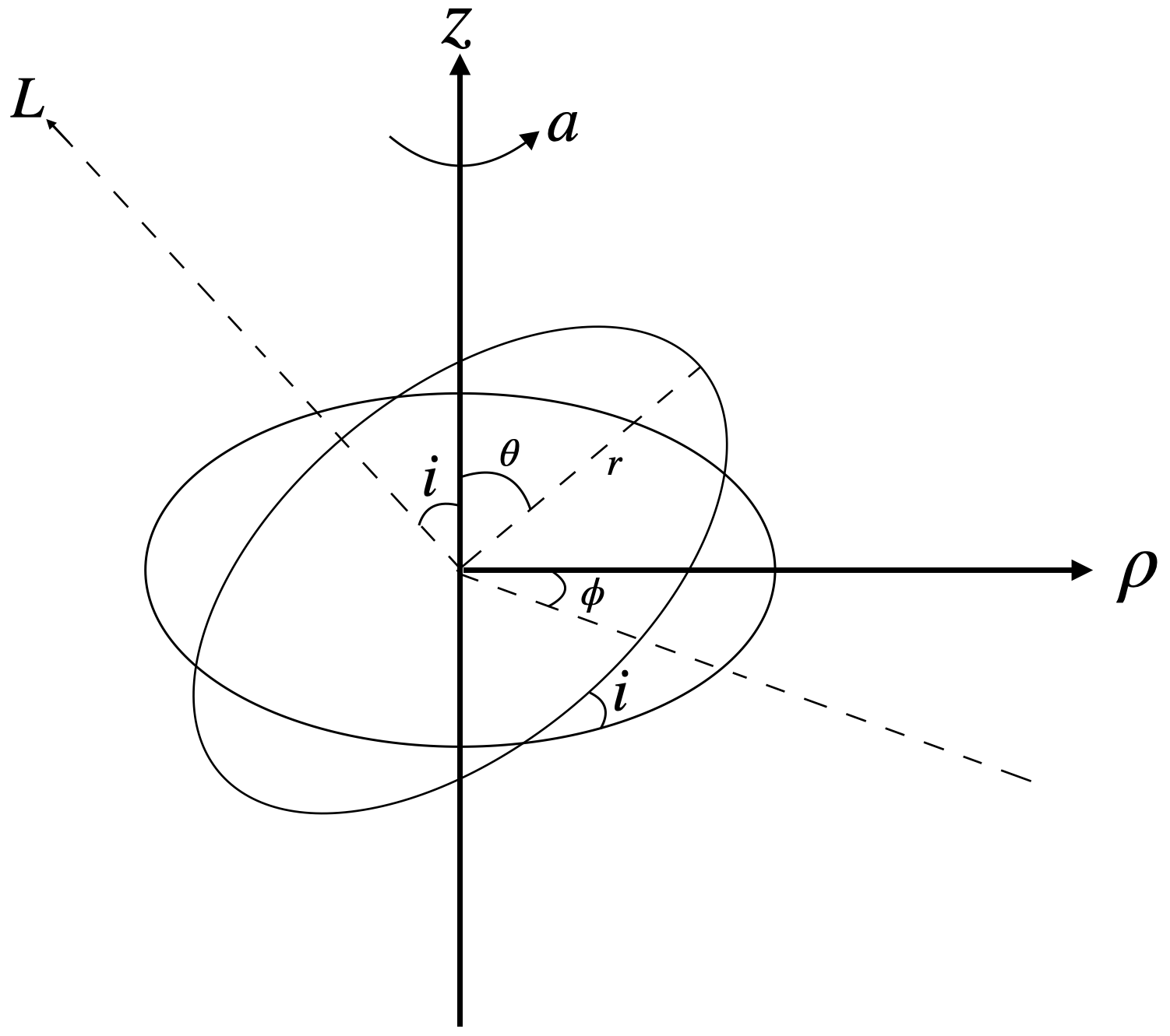
Figure 1: Different dynamical parameters of an off-equatorial orbit around a COP. The inclined plane consists of a circular orbit along which the test particle rotates. The orbit is inclined at an angle $i$ with the symmetry axis of the COP (the $z$-axis) and its equatorial plane. The rotation parameter of the COP is $a$. $L$ denotes the total angular momentum of the test particle, and its direction is along the rotating axis of the inclined orbit.

If a particle of unit mass is accreting around a rotating COP of mass $M_{\text{BH}}$ and angular momentum $J_{\phi}$ on a plane inclined at an angle $i$ with the equatorial plane of the COP (Figure 1), the generalised gravitational force on the particle, as prescribed in Ghosh and Mukhopadhyay [2], can be mimicked by the expression

$$F_{\text{GM}r}=\frac{2\mathcal{A}^{2}\sec^{2}i}{\left[a\sqrt{2}r^{3/2}\left\{\Delta+2r\left(r-1\right)\right\}+r\Delta\sqrt{\left\{\mathcal{A}+r^{4}-a^{2}(\Delta+r^{2}-3r)\right\}\cos 2i\sec^{2}i}\right]^{2}}$$ (1)

where $\mathcal{A}=a^{4}+r^{4}+2a^{2}r(r-2)$ and $\Delta=r^{2}+a^{2}-2r$. The Kerr parameter $a=J_{\phi}/M_{\text{BH}}$ denotes the rotation parameter of the COP, such that $a\in[-1,1)$. Here, $r$ is the radial distance of the rotating particle from the origin in the spherical polar coordinate $(r,\theta,\phi)$. The gravitational force on the particles, given in equation (1), can be applied successfully by taking the value of $i$ in the range $i\in[0^{\circ},30^{\circ}]$ while keeping the error within a reasonable limit, and maintaining a resemblance with the actual physical scenario [2]. The corresponding pseudo-Kerr potential $V_{\text{GM}}$, for particular values of $a$ and $i$, can be evaluated from the generalised force using the relation

$$V_{\text{GM}}(r,a,i)=-\int_{r}^{\infty}F_{\text{GM}r}(r^{\prime},a,i)dr^{\prime}$$ (2)

For Schwarzschild-like COP s, the value of $a$ becomes $0$. Thus, by putting $a=0$ in the equation (2), we get the PNP for the inclined orbits around a Schwarzschild-like COP, which is given by

$$V_{\text{GMS}}(r)=-\frac{\sec(2i)}{r-2}$$ (3)

It should be mentioned that throughout the work, the velocities have been scaled by $c$, the speed of light in vacuum, and the distances are scaled by $r_{\text{g}}=GM_{\text{BH}}/c^{2}$, where $G$ is the gravitational constant. We have scaled all the parameters such that $G=M_{\text{BH}}=c=1$.

The potential, given in equation (3), is strikingly similar to the PNP presented in Paczynsky and Wiita [3]. By putting $i=0$, $V_{\text{GMS}}$ gets equal to the PW potential. The fact that $V_{\text{GM}}$ comes down to the PW PNP for $a=i=0$ signifies the generic nature of the GM PNP. Similarly, if we put $i=0$ but $a\neq 0$, we get the PNP for the orbits on the equatorial plane in the Kerr geometry.

The analytically closed form of the generalised PNP $V_{\text{GM}}$, however, is complicated to derive by a straightforward integration, as per the expression given in equation (2), because of the complex mathematical form of the gravitational force, given in equation (1). Therefore, we take a numerical approach where we integrate the generalised force $F_{\text{GM}r}$ numerically for several values of $r$ and fit the data with a fitting function of the form

$$V_{\text{GMf}}(r)=-\frac{\exp\left(\frac{\gamma_{1}}{(r-\gamma_{2})^{\gamma_{3}}}+\gamma_{4}\right)}{(r-\gamma_{2})^{\gamma_{5}}}$$ (4)

where $\gamma_{1},\gamma_{2},\gamma_{3},\gamma_{4}$, and $\gamma_{5}$ are fitting parameters. It is evident that the potential $V_{\text{GMf}}$ is spherically symmetric, similar to the potential $V_{\text{GM}}$. The fitting function asymptotically approaches zero when the test particle moves towards infinity $\left(V_{\text{GMf}}\rightarrow 0\text{, when }r\rightarrow\infty\right)$. Also, it tends to infinity when the test particle approaches the event horizon at the radial distance $r=\gamma_{2}r_{\text{g}}$ $\left(V_{\text{GMf}}\rightarrow-\infty\text{, when }r\rightarrow\gamma_{2}\right)$. Moreover, the function $V_{\text{GMf}}$ fits with the PNP $V_{\text{GM}}$ efficiently with a minimal relative error, keeping the radii of the ISCO $R_{\text{ISCO}}$, and the marginally bound orbit $R_{\text{mb}}$ to be almost same as that in the Kerr geometry. These facts satisfy the conditions of a PNP, and it leads us to implement $V_{\text{GMf}}$, given in equation (4), as a suitable fitting function. For particular values of $a$ and $i$, the fitting parameters are evaluated so that $V_{\text{GMf}}$ fits with $V_{\text{GM}}$, and after that we can use the fitting function as an independent PNP.

As there is azimuthal symmetry in the orbital motion of the particle revolving around a COP, it is convenient to write equation (4) in the cylindrical polar coordinates $(\rho,\phi,z)$ as

$$V_{\text{GMf}}(\rho,z)=-\frac{\exp\left(\frac{\gamma_{1}}{\left(\sqrt{\rho^{2}+z^{2}}-\gamma_{2}\right)^{\gamma_{3}}}+\gamma_{4}\right)}{\left(\sqrt{\rho^{2}+z^{2}}-\gamma_{2}\right)^{\gamma_{5}}}$$ (5)

The absence of any $\phi$ term in the potential signifies the azimuthal symmetry. Section 3.2.2 presents more details about the fitting function.

As the GM PNP is generic in nature, it is worthwhile to ask how this potential will behave for the orbits on the equatorial plane around a rotating COP ($i=0$ but $a\neq 0$) and how this potential differs from any other PNP which is being applied in this scenario. We consider the well-known ABN PNP to draw a comparison with GMf PNP for $i=0$.

The ABN PNP, after integrating the free-fall acceleration prescribed in Artemova et al. [1], comes out to be

$$V_{\text{ABN}}(r)=-\frac{1}{r_{1}(\beta-1)}\left[\frac{r^{\beta-1}}{(r-r_{1})^{\beta-1}}-1\right]$$ (6)

Here, $r_{1}$ represents the radius of the event horizon, given as follows.

$$r_{1}=1+\sqrt{1-a^{2}}$$ (7)

The value of $\beta$ is given by

$$\beta=\frac{r_{\text{in}}}{r_{1}}-1$$ (8)

where $r_{\text{in}}$ is the radius of ISCO such that

$$r_{\text{in}}=3+Z_{2}\mp\sqrt{(3-Z_{1})(3+Z_{1}+2Z_{2})}$$ (9)

The values of the parameters $Z_{1}$ and $Z_{2}$ are defined as

$$Z_{1}=1+(1-a^{2})^{\frac{1}{3}}\left[(1+a)^{\frac{1}{3}}+(1-a)^{\frac{1}{3}}\right]\text{ and }Z_{2}=\sqrt{3a^{2}+Z_{1}^{2}}$$ (10)

The negative and positive signs in equation (9) signify the co-rotating ($a>0$) and counter-rotating ($a<0$) COP s, respectively.

Along with the monopole term represented by any of the PNP s, which is conservative, we use a dipolar, non-central, perturbative term, which is introduced to simulate a halo far from the central object. The distribution of the halo is such that it is axially symmetric about the rotating axis of the COP. If the halo is also symmetric about the equatorial plane, the first non-central, contributing term in the potential will be quadrupolar in nature [14, 58]. However, we consider the halo to be asymmetrically placed about the equatorial plane, somewhat deformed in the polar regions [63]. In this case, the non-central, leading term will be dipolar, which can be represented with a potential

$$\psi_{\text{dip}}=\mathcal{D}rP_{1}(\cos\theta)=\mathcal{D}z$$ (11)

Here, $\mathcal{D}$ is the dipole coefficient, $P_{n}(x)$ is the Legendre polynomial of degree $n$, $\cos\theta=z/r$, and $r^{2}=\rho^{2}+z^{2}$. The value of $\mathcal{D}$ will depend on the asymmetry in the mass distribution of the halo, and it will be small for any practical system [14, 4]. Therefore, the net potential that the particle experiences while revolving around a COP surrounded by an asymmetrically distributed halo can be represented by a linear superposition of the potentials, i.e.,

$$\Phi_{\text{g}}(\rho,z)=V_{\text{PNP}}(\rho,z)+\psi_{\text{dip}}$$ (12)

The pseudo-potential term $V_{\text{PNP}}$ in equation (12) will be replaced by either of the monopole terms, which is $V_{\text{GM}}$, $V_{\text{GMS}}$, $V_{\text{GMf}}$, or $V_{\text{ABN}}$, depending on the nature of the COP under consideration. The linear nature of the Newtonian framework allows the superposition of the potentials, in this case [58].

The orbit of the test particle, with specific angular momentum $L$, is inclined with respect to the equatorial plane with an inclination angle $i$, and it is precessing about the spinning axis of the COP. This phenomenon is known as the Lense-Thirring Precession [62]. The $z$-component of the angular momentum $L_{z}$ is conserved due to the azimuthal symmetry of the orbit. The locus of the particle will not always make an angle $i$ with the equatorial plane. Still, the plane of orbital precession will always be inclined at $i$ with the spinning axis of the COP (Figure 1). Therefore, $L_{z}=L\cos i$, which implies that $L$ is also conserved [2].

The motion of the orbiting particle in the $\phi$ direction will induce a centrifugal force on it along the radial direction. This can be taken into account by adding a term $\left(\dfrac{L^{2}}{2\rho^{2}}\right)$ with the potential $\Phi_{\text{g}}(\rho,z)$ in equation (12). Hence, the following expression can describe the effective potential in Kerr geometry.

$$\left.V_{\text{eff}}(\rho,z)\right|_{a\neq 0}=-\frac{\exp\left(\frac{\gamma_{1}}{\left(\sqrt{\rho^{2}+z^{2}}-\gamma_{2}\right)^{\gamma_{3}}}+\gamma_{4}\right)}{\left(\sqrt{\rho^{2}+z^{2}}-\gamma_{2}\right)^{\gamma_{5}}}+\mathcal{D}z+\frac{L^{2}}{2\rho^{2}}$$ (13)

The net potential for an off-equatorial orbit in Schwarzschild geometry $(a=0)$ is more straightforward. We can use the potential given in equation (3) and write down the net effective potential as follows.

$$\left.V_{\text{eff}}(\rho,z)\right|_{a=0}=-\frac{\sec(2i)}{\sqrt{\rho^{2}+z^{2}}-2}+\mathcal{D}z+\frac{L^{2}}{2\rho^{2}}$$ (14)

The dynamics of the test particle will be governed by these effective potentials, the choice of which depends on the type of COP it is rotating around.

2.2 Equations of motion

We move on to formulating the equations of motion for our system. The equations of motion of the test particle can be derived from the non-dimensional Hamiltonian [64, 58], given by

$$H=\frac{1}{2}\left(p_{\rho}^{2}+p_{z}^{2}\right)+V_{\text{eff}}(\rho,z)$$ (15)

where $V_{\text{eff}}$ can be replaced by either the potential given in equation (13) for a Kerr-like COP or the one given in equation (14) for a Schwarzschild-like COP. Thus, the equations of motion can be formulated as follows.

$$\dot{\rho}=p_{\rho}$$ (16a)

$$\dot{p_{\rho}}=-\frac{\partial V_{\text{eff}}}{\partial\rho}=-\frac{\partial\Phi_{\text{g}}}{\partial\rho}+\frac{L^{2}}{\rho^{3}}$$ (16b)

$$\dot{z}=p_{z}$$ (16c)

$$\dot{p_{z}}=-\frac{\partial V_{\text{eff}}}{\partial z}=-\frac{\partial\Phi_{\text{g}}}{\partial z}$$ (16d)

Here, there is no special relativistic correction as the particle’s speed is assumed to be much less than $c$. The energy of the test particle is given by $E=\sqrt{1+2E_{\text{mech}}}$, where

$$E_{\text{mech}}=\frac{1}{2}\left(p_{\rho}^{2}+p_{z}^{2}\right)+\Phi_{\text{g}}(\rho,z)+\frac{L^{2}}{2\rho^{2}}$$ (17)

Therefore, the conservation equation can be written as

$$E^{2}-p_{\rho}^{2}-p_{z}^{2}-2\Phi_{\text{g}}-\frac{L^{2}}{\rho^{2}}=1$$ (18)

From equation (18), it can be concluded that the motion of the test particle will be restricted by $E^{2}-2\Phi_{\text{g}}-\dfrac{L^{2}}{\rho^{2}}-1\geq 0$, which is a direct consequence of the conservation of energy and angular momentum.

However, if the speed of the particle is comparable to the speed of light, special relativistic corrections to the equations in (16a-16d) have to be performed [4, 54]. We consider the non-dimensional Lagrangian of the relativistic particle $\mathcal{L}=-\dfrac{1}{\gamma}-\Phi_{\text{g}}$, where the term $\gamma$ is given by

$$\gamma=\frac{1}{\sqrt{1-\left(\dot{\rho}^{2}+\rho^{2}\dot{\phi}^{2}+\dot{z}^{2}\right)}}$$

The energy of the particle will be $E=\gamma+\Phi_{\text{g}}$, and the angular momentum of the particle will be $L=\dfrac{\partial\mathcal{L}}{\partial\dot{\phi}}=\gamma\rho^{2}\dot{\phi}$. The Lagrange’s equations for $\rho$ and $z$ can be found as

$$\left(\Phi_{\text{g}}-E\right)\ddot{\rho}=\frac{\partial\Phi_{\text{g}}}{\partial\rho}\left(1-\dot{\rho}^{2}\right)-\frac{\partial\Phi_{\text{g}}}{\partial z}\dot{\rho}\dot{z}-\frac{L^{2}}{(E-\Phi_{\text{g}})\rho^{3}}$$ (19a)

$$\left(\Phi_{\text{g}}-E\right)\ddot{z}=\frac{\partial\Phi_{\text{g}}}{\partial z}\left(1-\dot{z}^{2}\right)-\frac{\partial\Phi_{\text{g}}}{\partial\rho}\dot{\rho}\dot{z}$$ (19b)

As we have considered the test particle of unit mass, we can write $\dot{\rho}=p_{\rho}$ and $\dot{z}=p_{z}$. Thus, the relativistic equations of motion turn out to be

$$\dot{\rho}=p_{\rho}$$ (20a)

$$\dot{p_{\rho}}=\frac{1}{\Phi_{\text{g}}-E}\left[\frac{\partial\Phi_{\text{g}}}{\partial\rho}\left(1-p_{\rho}^{2}\right)-\frac{\partial\Phi_{\text{g}}}{\partial z}p_{z}p_{\rho}-\frac{L^{2}}{(E-\Phi_{\text{g}})\rho^{3}}\right]$$ (20b)

$$\dot{z}=p_{z}$$ (20c)

$$\dot{p_{z}}=\frac{1}{\Phi_{\text{g}}-E}\left[\frac{\partial\Phi_{\text{g}}}{\partial z}\left(1-p_{z}^{2}\right)-\frac{\partial\Phi_{\text{g}}}{\partial\rho}p_{z}p_{\rho}\right]$$ (20d)

From the expressions of energy $E$ and angular momentum $L$, along with the relation $u^{\mu}u_{\mu}=1$, the conservation equation can be evaluated as

$$p_{\rho}^{2}+p_{z}^{2}+\frac{L^{2}}{(E-\Phi_{\text{g}})^{2}\rho^{2}}+\frac{1}{(E-\Phi_{\text{g}})^{2}}=1$$ (21)

Similar to the non-relativistic case, the motion of the relativistic test particle will be restricted within the region governed by $1-\dfrac{L^{2}}{(E-\Phi_{\text{g}})^{2}\rho^{2}}-\dfrac{1}{(E-\Phi_{\text{g}})^{2}}\geq 1$.

It is worth mentioning that similar to the velocities and distances, all the terms signifying the physical quantities have been scaled to make them non-dimensional. The time $t$ has been scaled as $ct/r_{\text{g}}$, the momentum $p$ has been scaled as $p/(\mu c)$, and the angular momentum has been scaled as $L/(\mu cr_{\text{g}})$, where $\mu$ is the mass of the test particle taken to be unity in our analysis.

The energy conservation equations, given in equation (18) for non-relativistic case and equation (21) for relativistic case, converts the 4-dimensional phase space consisting of $(\rho,p_{\rho},z,p_{z})$ into an effective 3-dimensional hypersurface consisting of $(\rho,p_{\rho},z)$. The value of $p_{z}$ is bound to satisfy equation (21) for a particular set of the values of $(\rho,p_{\rho},z)$. This provides comprehensibility in analysing the system and also gives the advantage of minimising errors in numerical calculations.

2.3 Comparison between GMf PNP and ABN PNP for equatorial orbits

Before implementing the GMf PNP in studying the off-equatorial orbits, it is essential to consider the PNP for the equatorial orbits by putting the inclination angle $i=0^{\circ}$. In this context, we compare the two pseudo-potentials, namely the GMf PNP and the ABN PNP, and investigate which is more appropriate for sustaining the essential aspects of general relativity. Both potentials reproduce the radii of the ISCO to be the same as that in the fully relativistic case. Both of them reproduce the values of the radii of marginally bound orbits ($R_{\text{mb}}$) and the energy of unit mass at the marginally stable orbits ($E_{\text{ms}}$) with similar accuracy. The margin of dissimilarity being significantly less, both the PNP s can be implemented efficiently to study the accretion dynamics of equatorial disks. However, the simpler mathematical form of ABN PNP makes it more comprehensive and convenient to implement in complicated mathematical problems, for example, the Hill problem [61]. For off-equatorial orbits, the GM PNP is possibly one of the mandatory choices despite having a complex mathematical form.

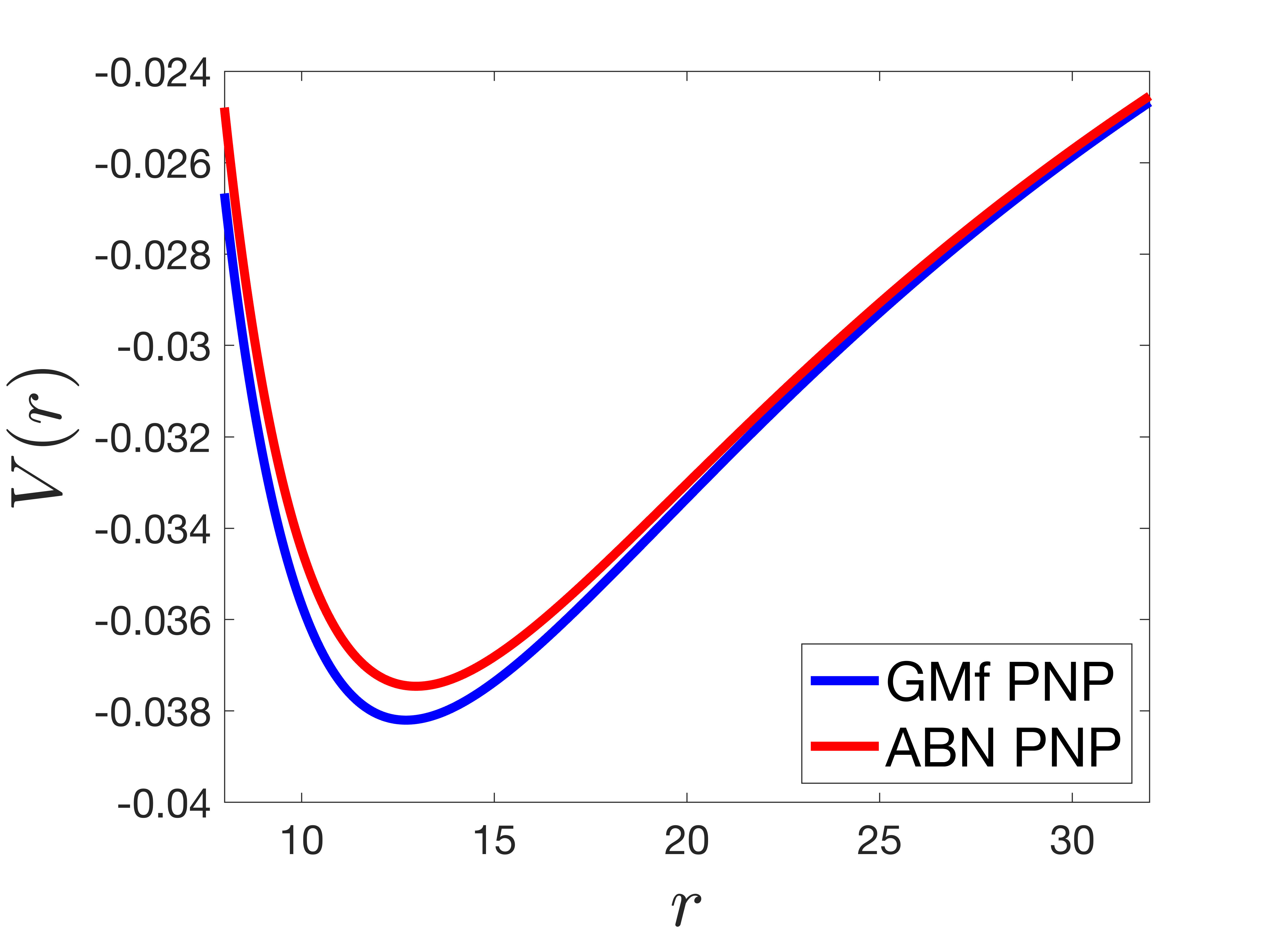
(a) $a$=0.1

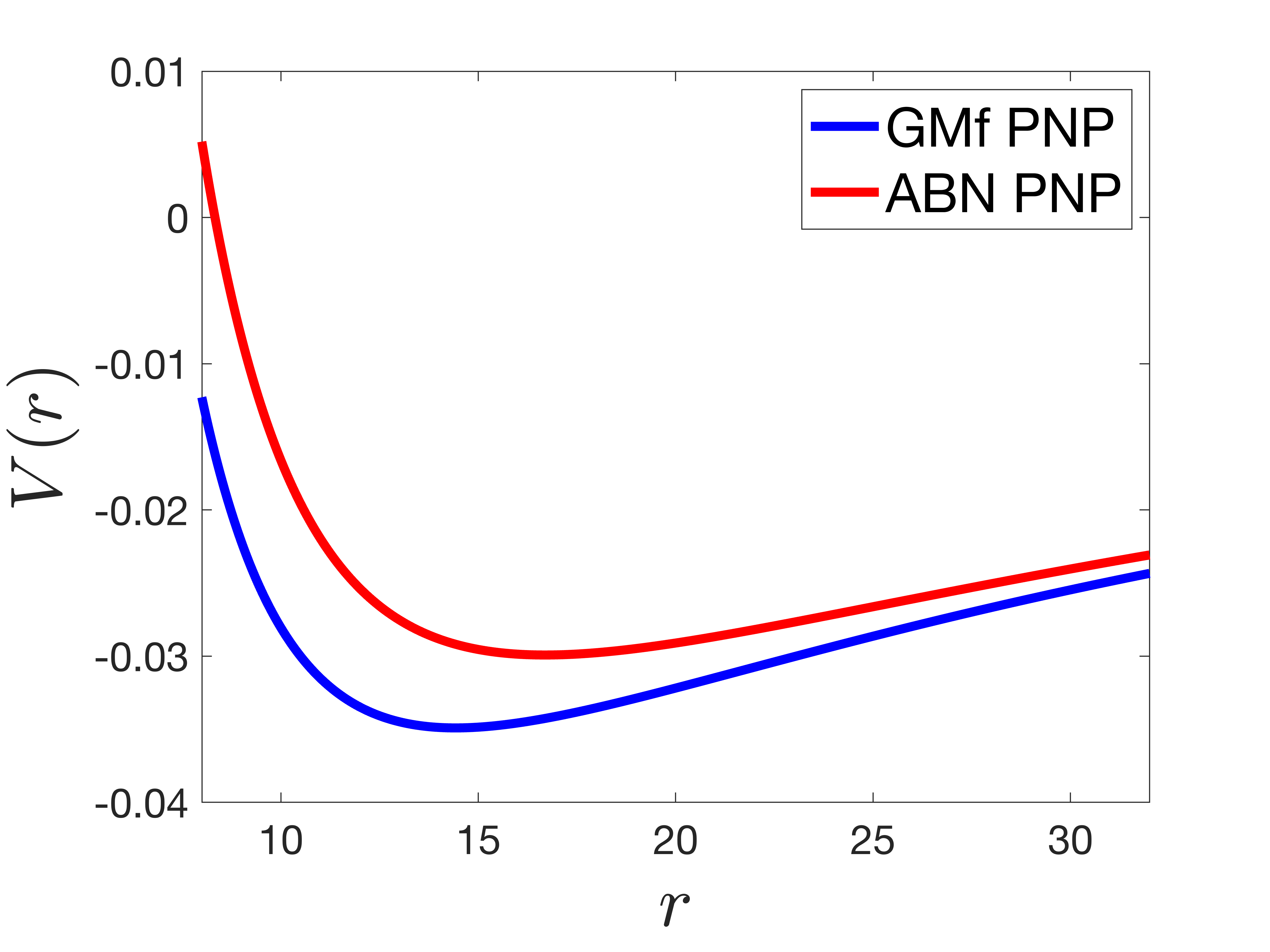
(b) $a$=0.9

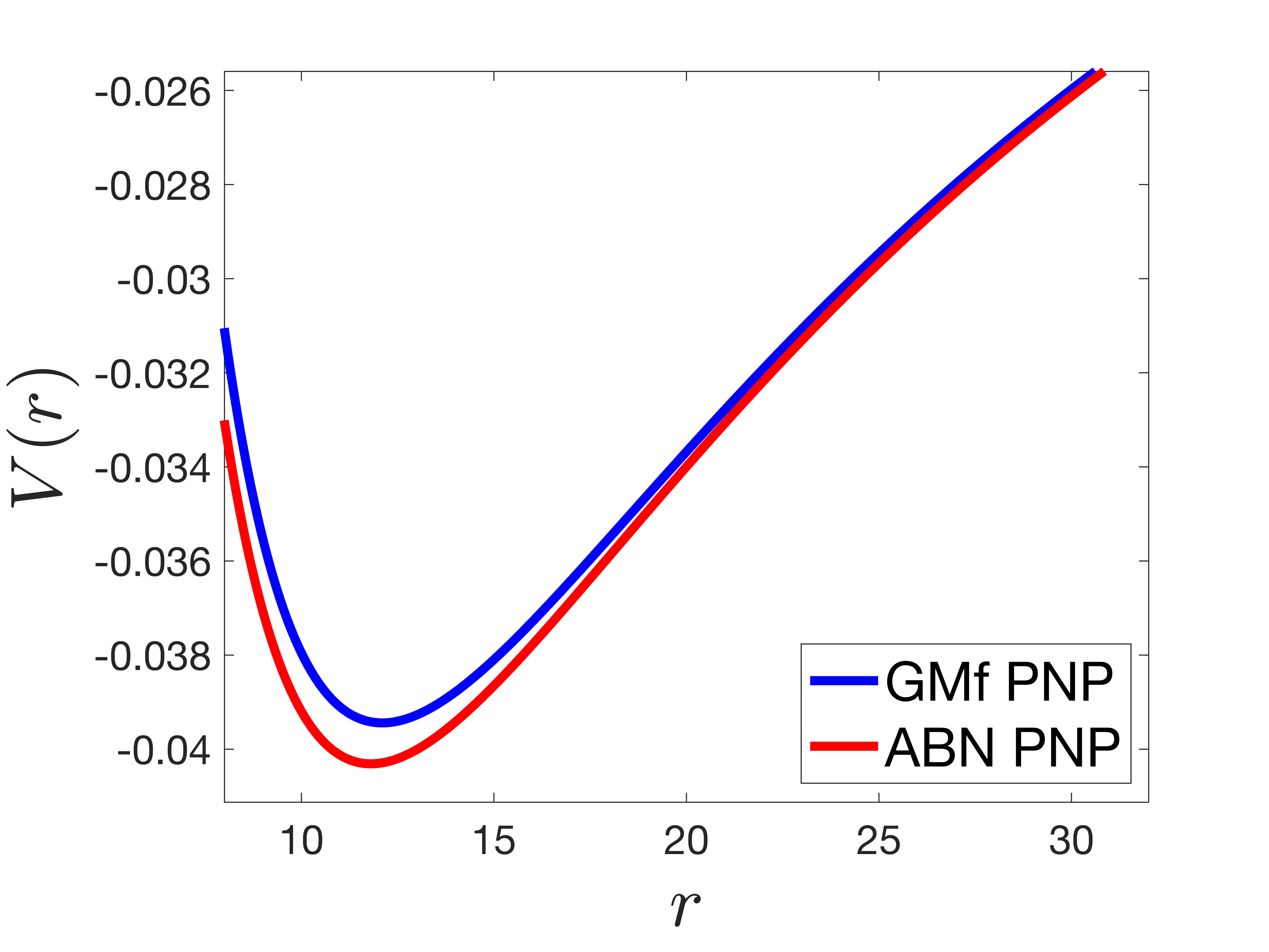
(c) $a$=-0.1

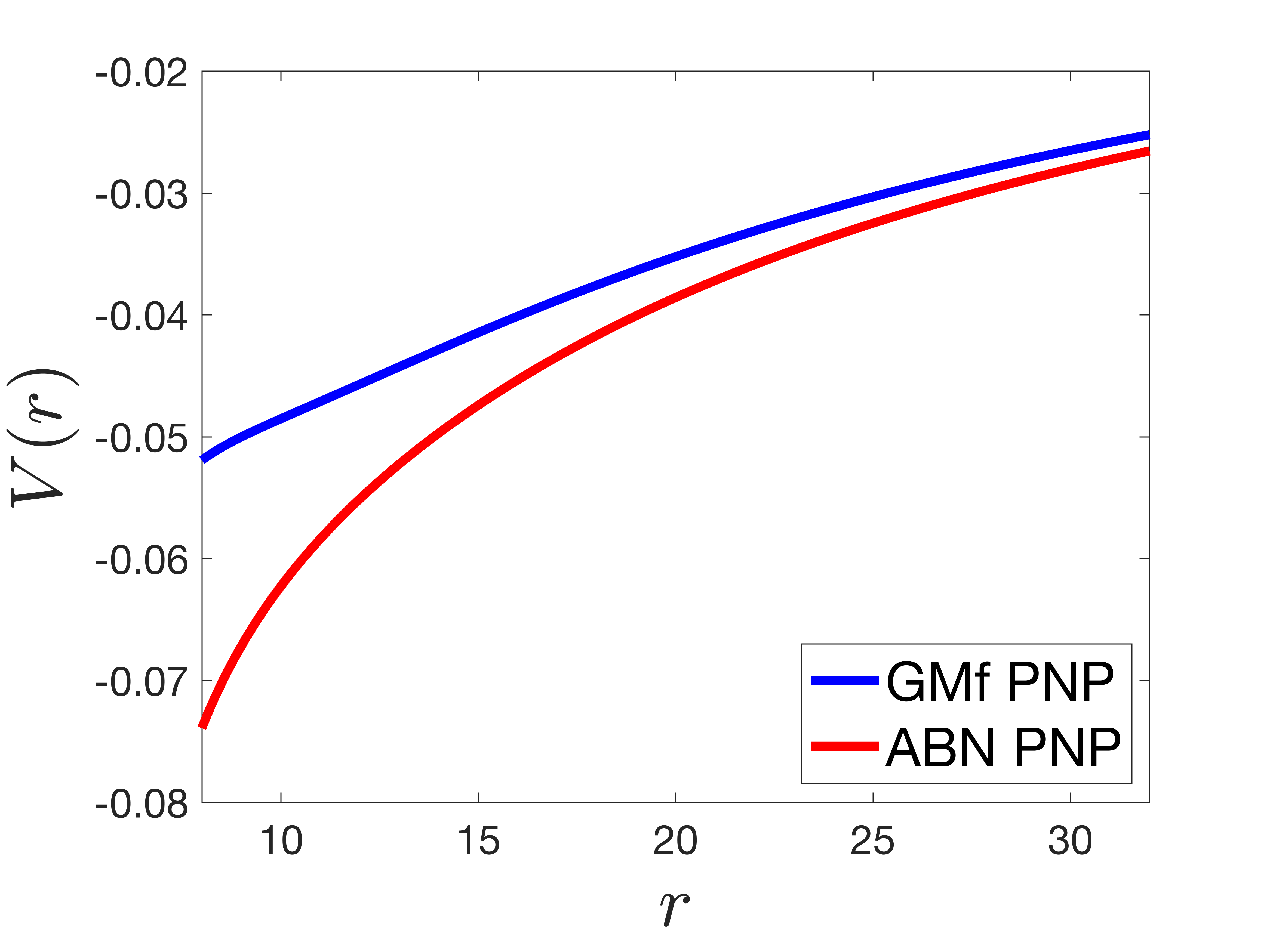
(d) $a$=-0.9

Figure 2: Comparison between the GMf PNP $\left(V(r)=V_{\text{GMf}}(r)+L^{2}/2r^{2}\right)$ and ABN PNP $\left(V(r)=V_{\text{ABN}}(r)+L^{2}/2r^{2}\right)$, for $z=0$, $L=4.2$, and different values of the Kerr parameter $a$.

If we find out the differences between the two PNP s at higher radial distances far from the event horizon, we can see a trend in their behaviour, which has a correlation with the rotation parameter $a$. Let us consider the effective potential $V(r)$ consisting of the GMf PNP $V_{\text{GMf}}(r)$, or the ABN PNP $V_{\text{ABN}}(r)$, along with the centrifugal contribution $\left(\dfrac{L^{2}}{2r^{2}}\right)$. At $a=0$, which represents a Schwarzschild-like COP, both the PNP s come down to the PW PNP. That is why both ABN PNP and GMf PNP are equal to each other for $a=0$. For $a>0$, which represents a co-rotating Kerr-like COP, the effective potential consisting of the ABN PNP is more than that of the GMf PNP (Figure 2(a)-2(b)). For $a<0$, which represents a counter-rotating Kerr-like COP, the situation is opposite (Figure 2(c)-2(d)). In this case, the effective potential consisting of the ABN PNP is less compared to that of the GMf PNP. This impacts the chaotic behaviour of the equatorial orbits in a certain way, which has been studied in section 3.

3 Stability of orbits and visualization of chaos

In this section, we analyse the dynamical behaviours of the orbits around Schwarzschild or Kerr-like COP. We begin with the special case of stable circular orbits. Thereafter, we move on to the behaviours of generic orbits, where the coexistence of order and chaos occurs naturally. We look for the transitions from order to chaos and establish how the chaoticity correlates with the orbital parameters qualitatively using the Poincaré sections of the orbits.

3.1 Dynamical analysis of circular orbits

A circular orbit essentially satisfies the relations $\dot{r}=0$ and $\dot{p_{r}}=0$. As the gravitational force corresponding to the PNP s is central in nature, we can expect stable circular orbits to exist around the COP s. However, the dipolar perturbation term in equation (12) restricts the stable circular orbits to exist on any plane other than the equatorial plane where the dipolar term vanishes as $z=0$. In the off-equatorial planes, the dipolar term disrupts the spherical symmetry of the system. However, we are also interested in considering the off-equatorial planes. Therefore, we suppress the dipolar term for the time being by putting $\mathcal{D}=0$ in equation (12).

For an orbit around a COP with specific values of $a$ and $i$ to be circular, the relation $\dfrac{\partial V_{\text{eff}}}{\partial r}=0$ is required to be satisfied. For it to be stable, the extremum has to be a minimum. Therefore, the condition for an orbit to be a stable circular orbit turns out to be

$$\frac{\partial V_{\text{eff}}}{\partial r}=0\text{, and }\frac{\partial^{2}V_{\text{eff}}}{\partial r^{2}}\geq 0$$ (22)

Instead of the inequality, if we equate the second relation in equation (22) with 0 and solve the equations simultaneously, the solution essentially gives the radius of the ISCO for given values of $a$ and $i$ [65].

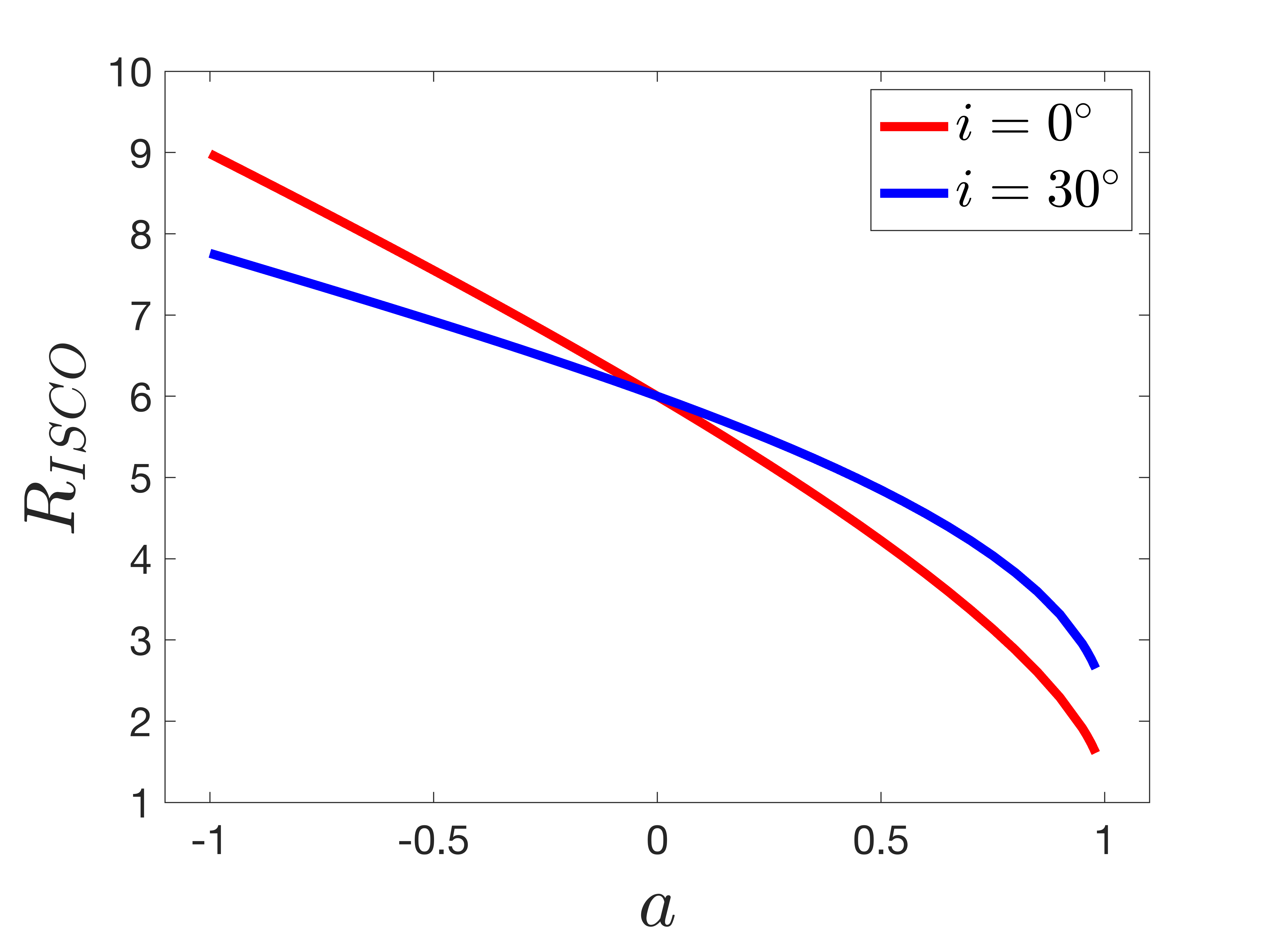
(a) $R_{\text{ISCO}}$ vs $a$, $i=0^{\circ}$, $30^{\circ}$

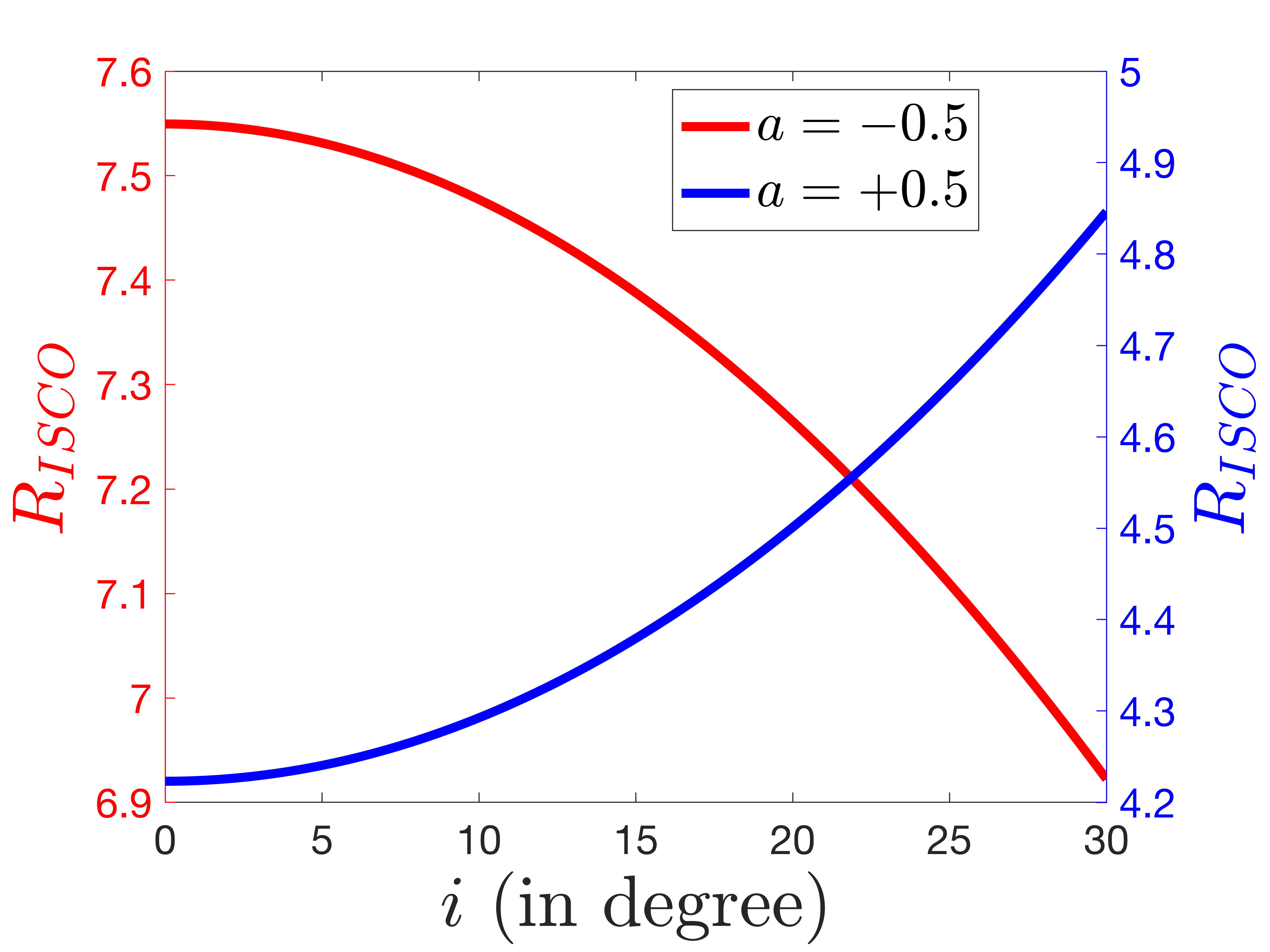
(b) $R_{\text{ISCO}}$ vs $i$, $a=\pm 0.5$

Figure 3: Correlations of the radii of ISCO s $\left(R_{\text{ISCO}}\right)$ with the Kerr parameter $a$ and the inclination angle $i$. The orbits are governed by the GMf PNP.

In Figure 3, we study how the radii of ISCO s vary with the rotation parameter of the COP $a$ and the inclination of the orbit $i$. At first, we observe that the change in $R_{\text{ISCO}}$ with respect to the Kerr parameter $a$ is significant for any angle of inclination, be it $i=0^{\circ}$, or $i=30^{\circ}$ (Figure 3(a)). For the equatorial orbits with $i=0^{\circ}$, the radii change from $9r_{\text{g}}$ to $\approx 1r_{\text{g}}$ in the span of $a\in[-1,1)$. The change in $R_{\text{ISCO}}$ with respect to $a$ for ABN PNP is precisely the same as that for GMf PNP. The value of $R_{\text{ISCO}}$ is almost linearly decreasing for most of the range of $a$, except for the orbits around the maximally co-rotating COP s (when $a\rightarrow 1$), in which case the change in $R_{\text{ISCO}}$ is more drastic. For $i=30^{\circ}$, the value of $R_{\text{ISCO}}$ varies in a similar way with $a$, although it changes from $7.76r_{\text{g}}$ to $\approx 2.5r_{\text{g}}$ in the span of $a\in[-1,1)$. For $a=0$, there is no change in the radius of ISCO as the inclination angle varies, and it remains unchanged at $R_{\text{ISCO}}=6r_{\text{g}}$. The result is expected for the Schwarzschild-like COP, as there is no rotation axis to identify the equatorial plane. Hence, all the planes are equivalent, and there is no special plane to impose larger or smaller stability on the circular orbits.

In Figure 3(b), we can see the dependence of $R_{\text{ISCO}}$ on the inclination angle $i$ for both co-rotating ($a>0$) and counter-rotating ($a<0$) COP s. In both cases, the change in the value of $R_{\text{ISCO}}$ in the range $i\in[0^{\circ},30^{\circ}]$ is small. For the orbits around the counter-rotating COP, the value of $R_{\text{ISCO}}$ decreases monotonically with $i$. On the contrary, it increases monotonically with the inclination angle for the orbits around the co-rotating COP s. The radii change more rapidly at the higher values of $i$ than at its lower values.

With the above analysis, we get a picture of the stable circular orbits in our system, including their dependence on the Kerr parameter $a$ and inclination angle $i$. We observed that the radii of ISCO s are significantly more influenced by $a$ than by $i$. For orbits around counter-rotating COP s, $R_{\text{ISCO}}$ decreases with $i$. On the other hand, it increases with $i$ for the orbits around the co-rotating COP s. For the Schwarzschild-like COP ($a=0$), $R_{\text{ISCO}}$ does not change with $i$. However, generic orbits are much more complicated and nuanced, requiring more detailed analysis and special tools to study their stability.

3.2 Dynamical analysis of generic orbits

We move on to the analysis of the generic orbits. We have implemented the method of Poincaré Map of the sections of phase space to visualise the change in chaos and order in the system qualitatively. In this method, instead of looking at the entire three-dimensional hypersurface $(\rho,p_{\rho},z)$, we look at a two-dimensional cross-section of the phase space, which consists of the points of intersection of the trajectories on a fixed plane (such as $z=0$) while moving in a particular direction along the trajectory [66]. The periodic orbits give rise to one or more isolated points on the sectional map, whereas the chaotic orbits give rise to a sea of scattered points [66, 67]. There can be other stable orbits, quasi-periodic regular orbits, which form systematic patterns in the map corresponding to the concentric Kolmogorov-Arnold-Moser (KAM) tori.

In this paper, we have plotted the Poincaré sections on the $z=0$ plane, while the orbits are moving out of the plane along their trajectories in the phase space. For a particular set of orbital parameters, the initial conditions, i.e., the coordinates $\rho(t=0)$, $z(t=0)$ and the momentum $p_{\rho}(t=0)$, are varied, and the value of $p_{z}(t=0)>0$ is evaluated from the conservation equation (18) for non-relativistic test particles and conservation equation (21) for relativistic test particles. We have studied the dependence of chaos on a particular parameter through a comparative study of the Poincaré maps by varying that parameter while keeping the rest fixed.

3.2.1 nonrotating compact object primaries

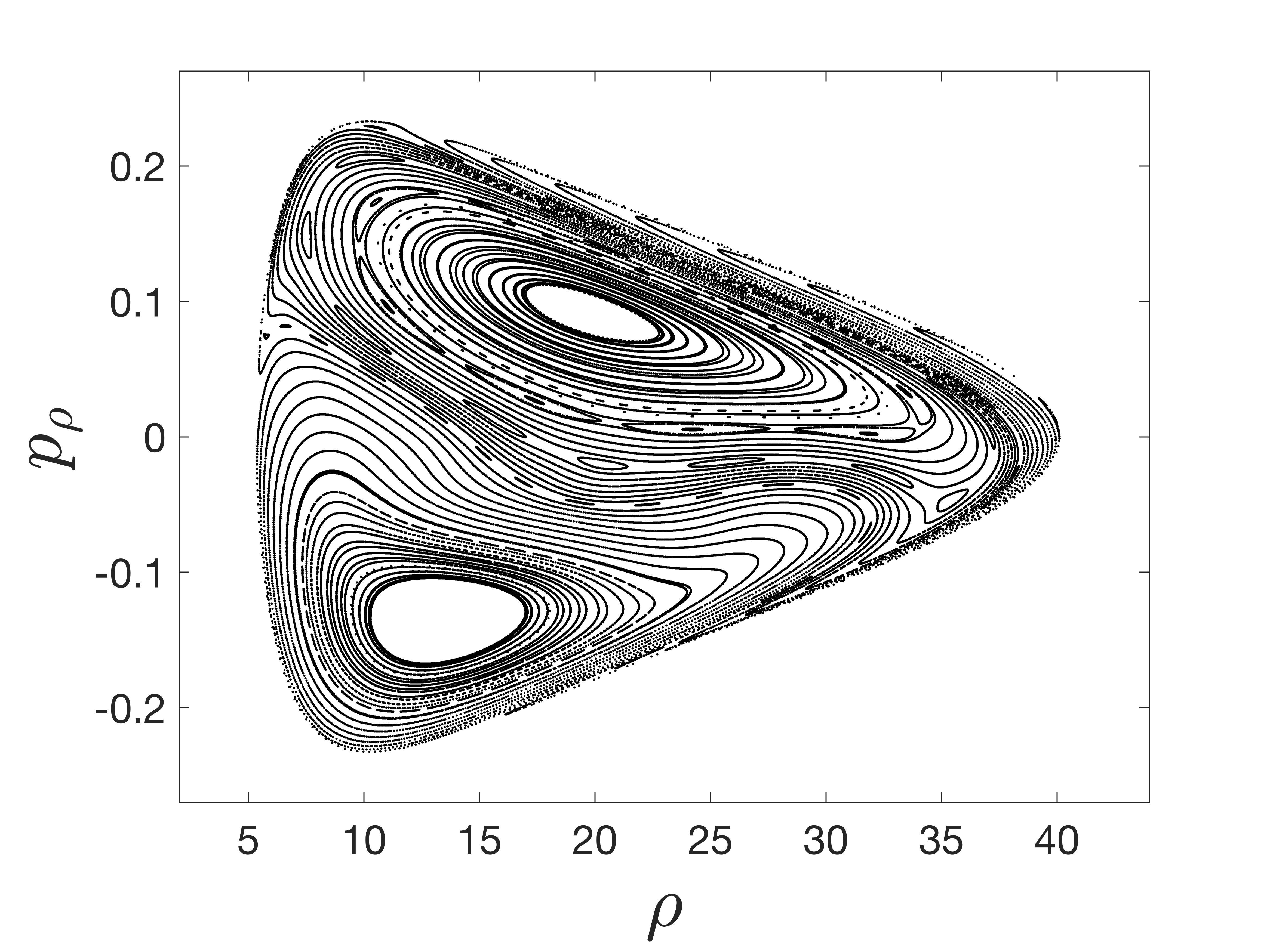
(a) $i=13^{\circ}$, Non-relativistic

(b) $i=15^{\circ}$, Non-relativistic

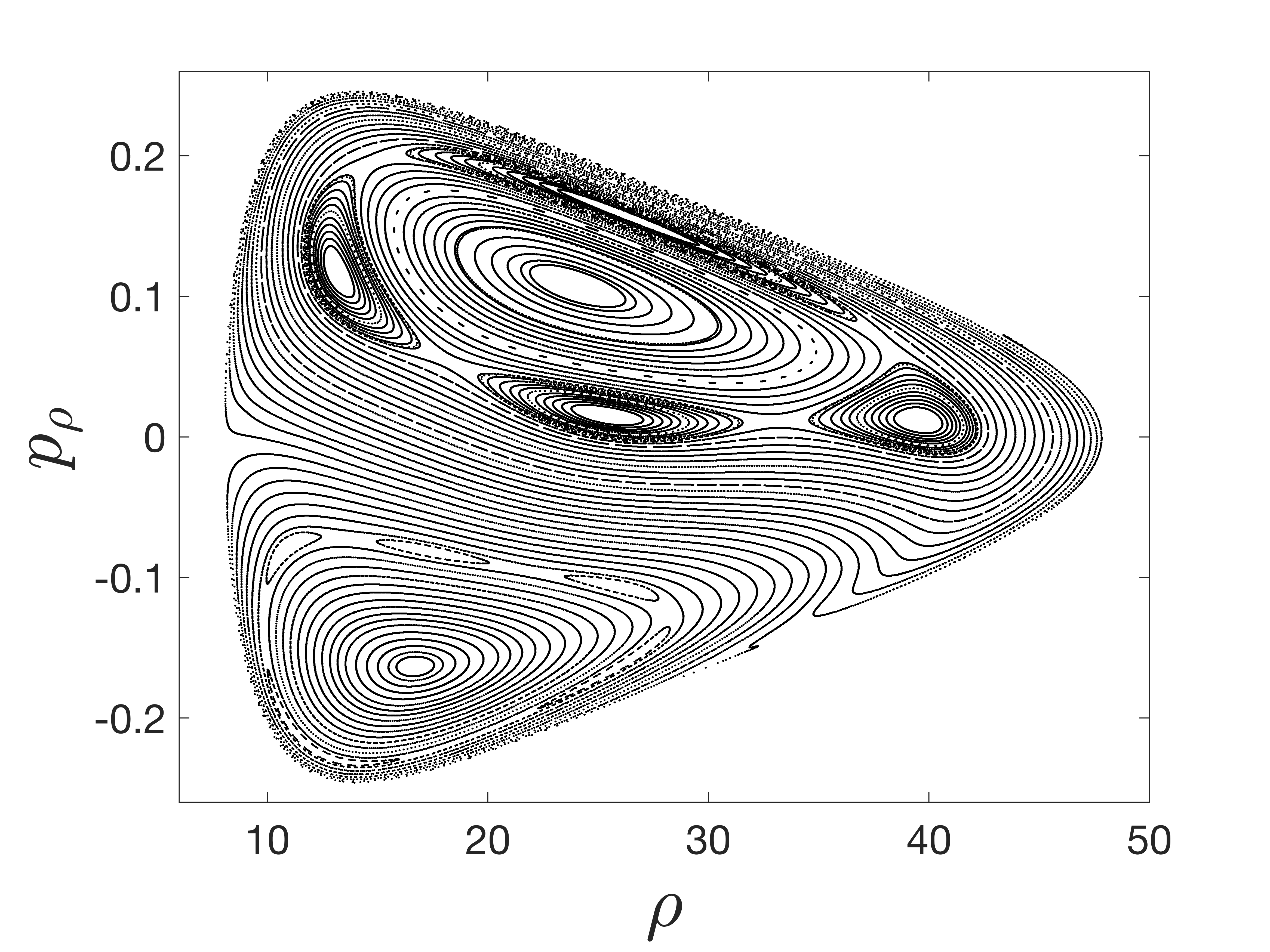
(c) $i=28^{\circ}$, Non-relativistic

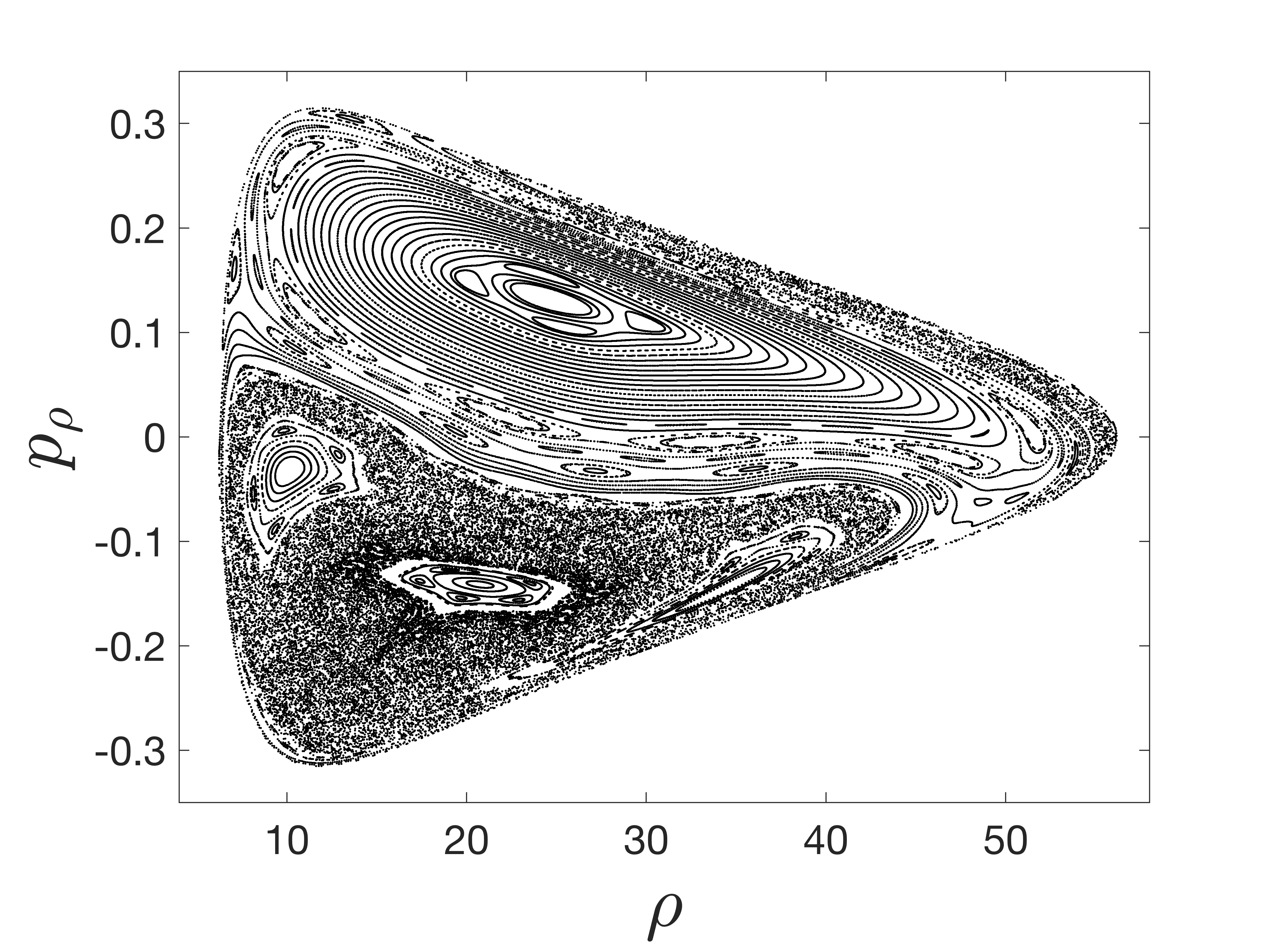
(d) $i=30^{\circ}$, Non-relativistic

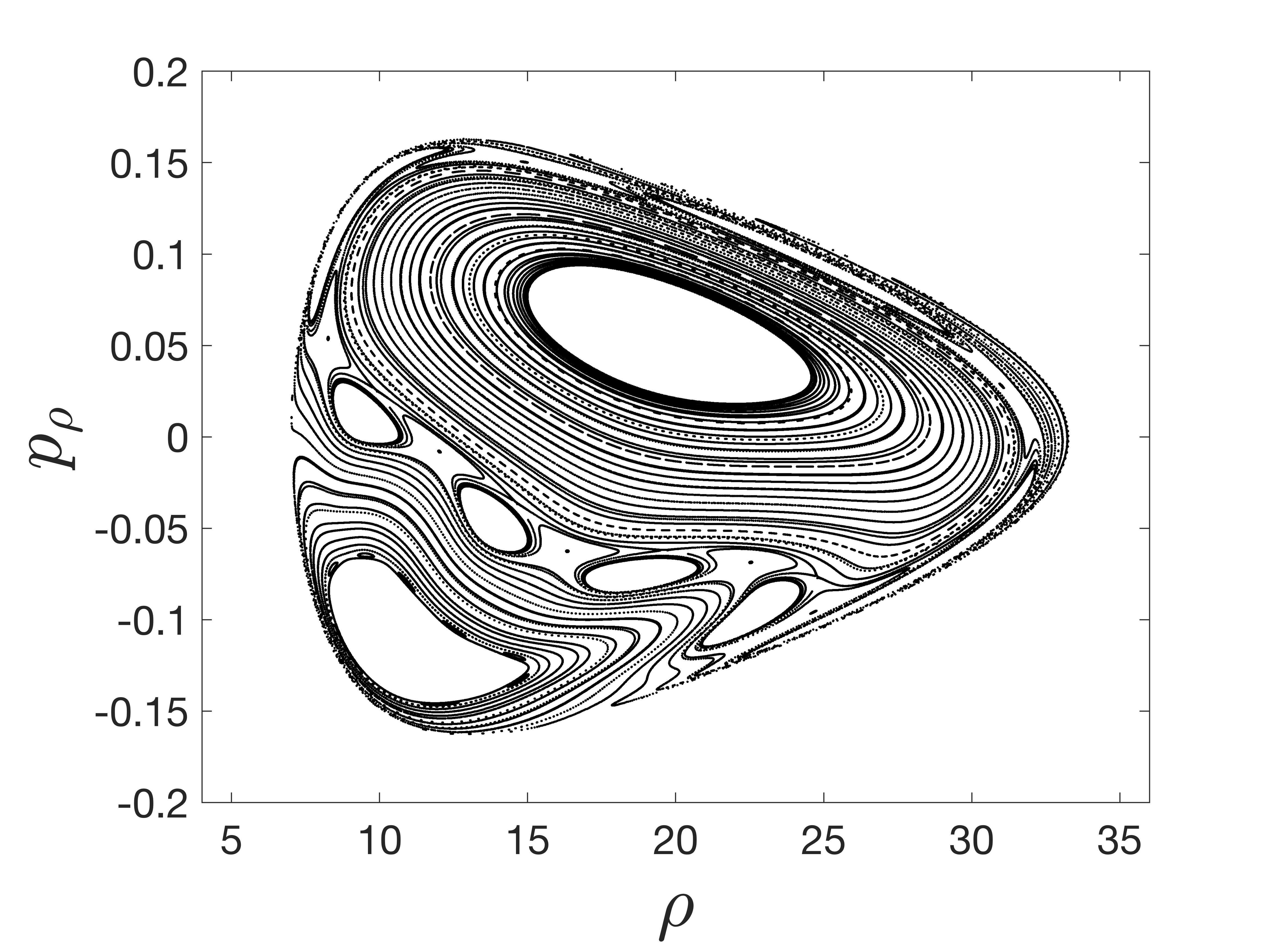
(e) $i=13^{\circ}$, Relativistic

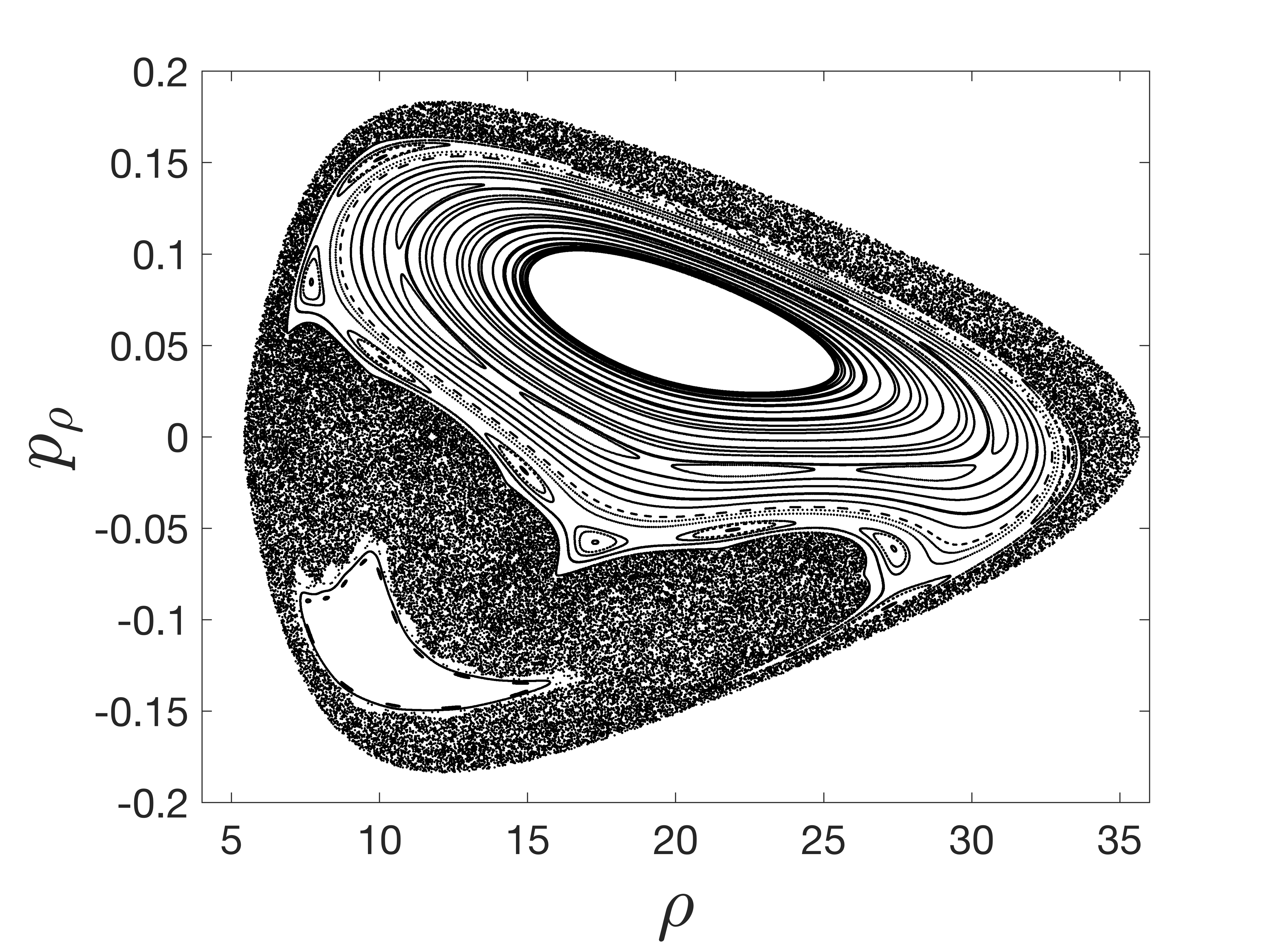
(f) $i=15^{\circ}$, Relativistic

Figure 4: Poincaré maps on the cross-sectional plane $z=0$ for the orbits governed by GMS PNP around nonrotating COP s ($a=0$). The inclination angle $i$ is varied. The parameters are (a)-(b) $E=0.976$, $L=4.20$, $\mathcal{D}=2\times 10^{-4}$, (c)-(d) $E=0.968$, $L=5.85$, $\mathcal{D}=2\times 10^{-4}$, and (e)-(f) $E=0.974$, $L=4.60$, $\mathcal{D}=2\times 10^{-4}$.

As the gravitational force, given in equation (1), is generic in nature, we can put $a=0$ in the expression and study the off-equatorial orbits around a static and stationary COP. We have implemented the effective potential consisting of GMS PNP, as given in equation (14), and worked out the equations of motion as per the equations given in (16a-16d) which does not consider any relativistic correction. We have varied the inclination angle $i$ and generated the Poincaré Maps for each of the angles. We have shown the maps for $i=13^{\circ},\text{ and }15^{\circ}$ by keeping the total energy $E$, total angular momentum $L$, and dipole coefficient $\mathcal{D}$ unchanged (Figures 4(a)-4(b)). Evidently, the Poincaré Map of the phase space for $i=15^{\circ}$ consists of a more chaotic region than that for $i=13^{\circ}$, in which case most of the orbits are regular in nature. We have also shown the cross-sectional maps for $i=28^{\circ},\text{ and }30^{\circ}$ by increasing the angular momentum and decreasing the total energy in order to suppress the chaos for convenience in visualisation (Figures 4(c)-4(d)). We can observe more chaotic regions on the map for $i=30^{\circ}$ compared to that for $i=28^{\circ}$. Therefore, this provides qualitative evidence that the degree of chaos has a positive correlation with the angle of inclination $i$ of the orbit.

To incorporate the relativistic corrections into the equations, we have derived the equations of motion using equations given in (20a-20d). We solved these equations too, to get the Poincaré Maps corresponding to the phase spaces of the orbits of relativistic test-particle and studied the trend of the degree of chaos with the inclination angle $i$ (Figures 4(e)-4(f)). Similar to the non-relativistic case, we have kept the parameters $E$, $L$, and $\mathcal{D}$ to be constant. We can observe the exact similar behaviour of the orbits, as we have seen in the non-relativistic case. The phase space becomes more chaotic when the inclination angle $i$ increases from $13^{\circ}$ to $15^{\circ}$. The only difference is that we have used a smaller value of $E$ and a higher value of $L$ to suppress the nonlinearity of the relativistic equations of motion (20a-20d) in comparison to the corresponding non-relativistic case (Figures 4(a)-4(b)). This is a consequence of the fact that the special-relativistic phase-space trajectories are more chaotic than the corresponding non-relativistic counterparts, which is well-established in the literature [54, 4].

3.2.2 Rotating compact object primaries

After considering the Schwarzschild geometry, we move on to the Kerr geometry, where the Kerr parameter $a$ is non-zero. In this case, for particular values of $a$ and $i$, we first evaluate the PNP $V_{\text{GM}}$ from equation (2) for several values of $r$, using the generalised force $F_{\text{GM}r}$ given in equation (1). After that, we take the natural log of the potential values to fit the data with the logarithmic form of the fitting function in equation (4), which is given by

$$\ln\left(-V_{\text{GMf}}(r)\right)=\left(\frac{\gamma_{1}}{(r-\gamma_{2})^{\gamma_{3}}}+\gamma_{4}\right)-\gamma_{5}\ln\left(r-\gamma_{2}\right)$$ (23)

This allows us to fit the curve more conveniently with minimal error and evaluate the fitting parameters. After we estimate the values of the fitting parameters, we can use them in equation (13) to get the overall potential consisting of the GMf PNP term for particular values of $a$ and $i$, along with the dipolar perturbation term and the centrifugal contribution as well. Thereafter, we implement this potential in the equations (16a)-(16d) and equations (20a)-(20d) to get the equations of motion for non-relativistic and relativistic cases, respectively.

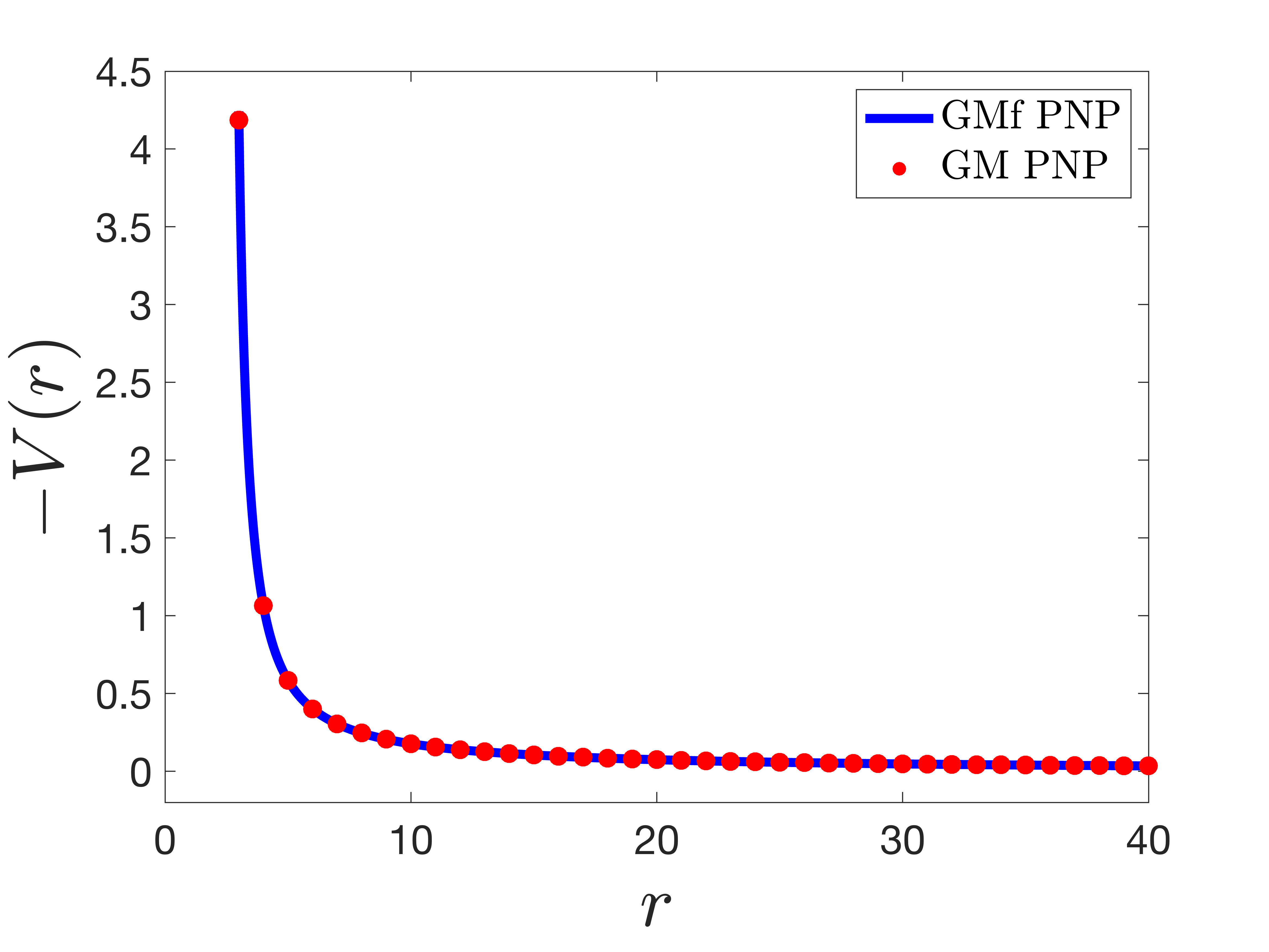
(a) $V_{\text{GM}}$ and $V_{\text{GMf}}$ for $a=-0.8$, $i=20^{\circ}$

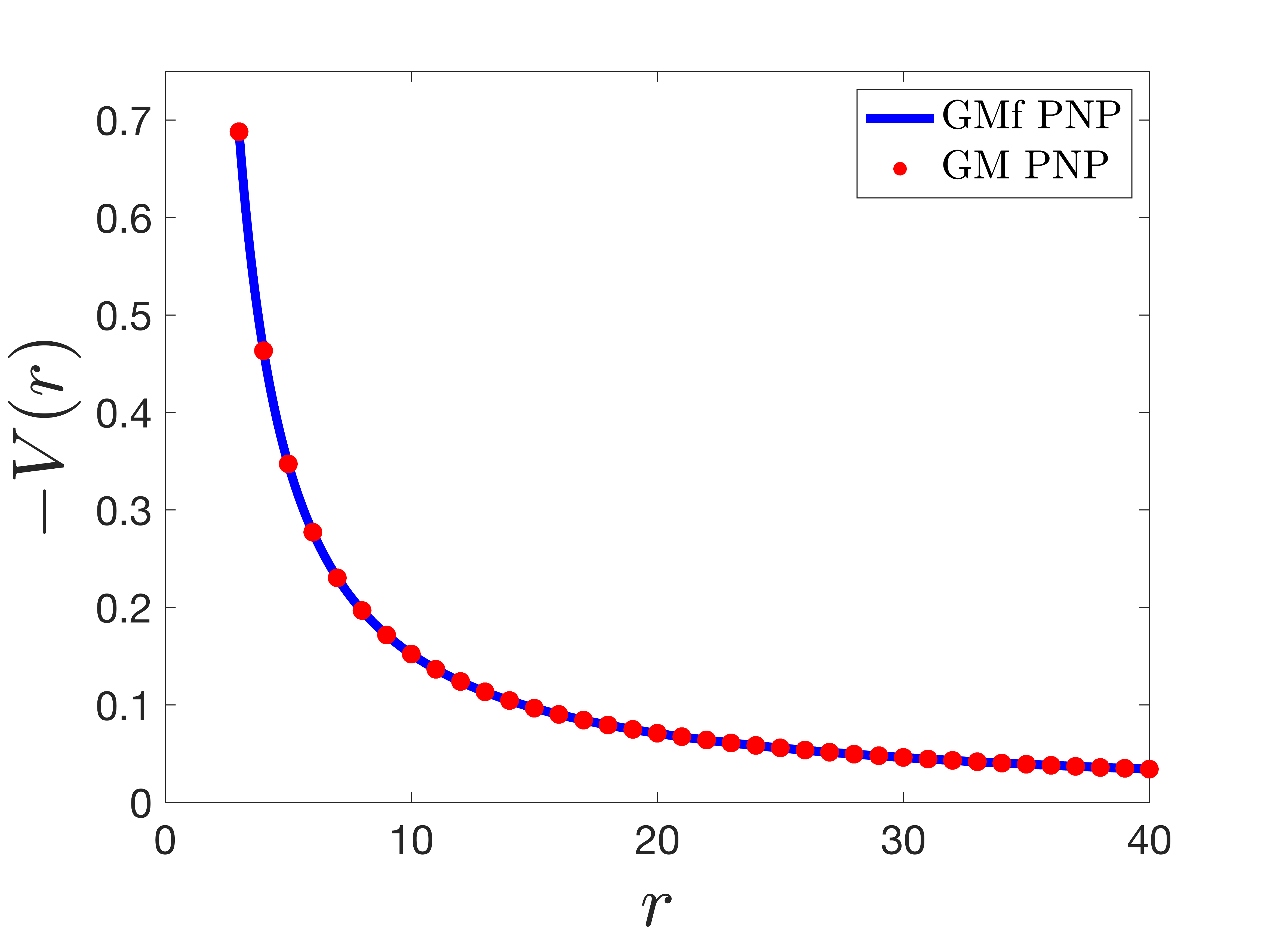
(b) $V_{\text{GM}}$ and $V_{\text{GMf}}$ for $a=0.8$, $i=20^{\circ}$

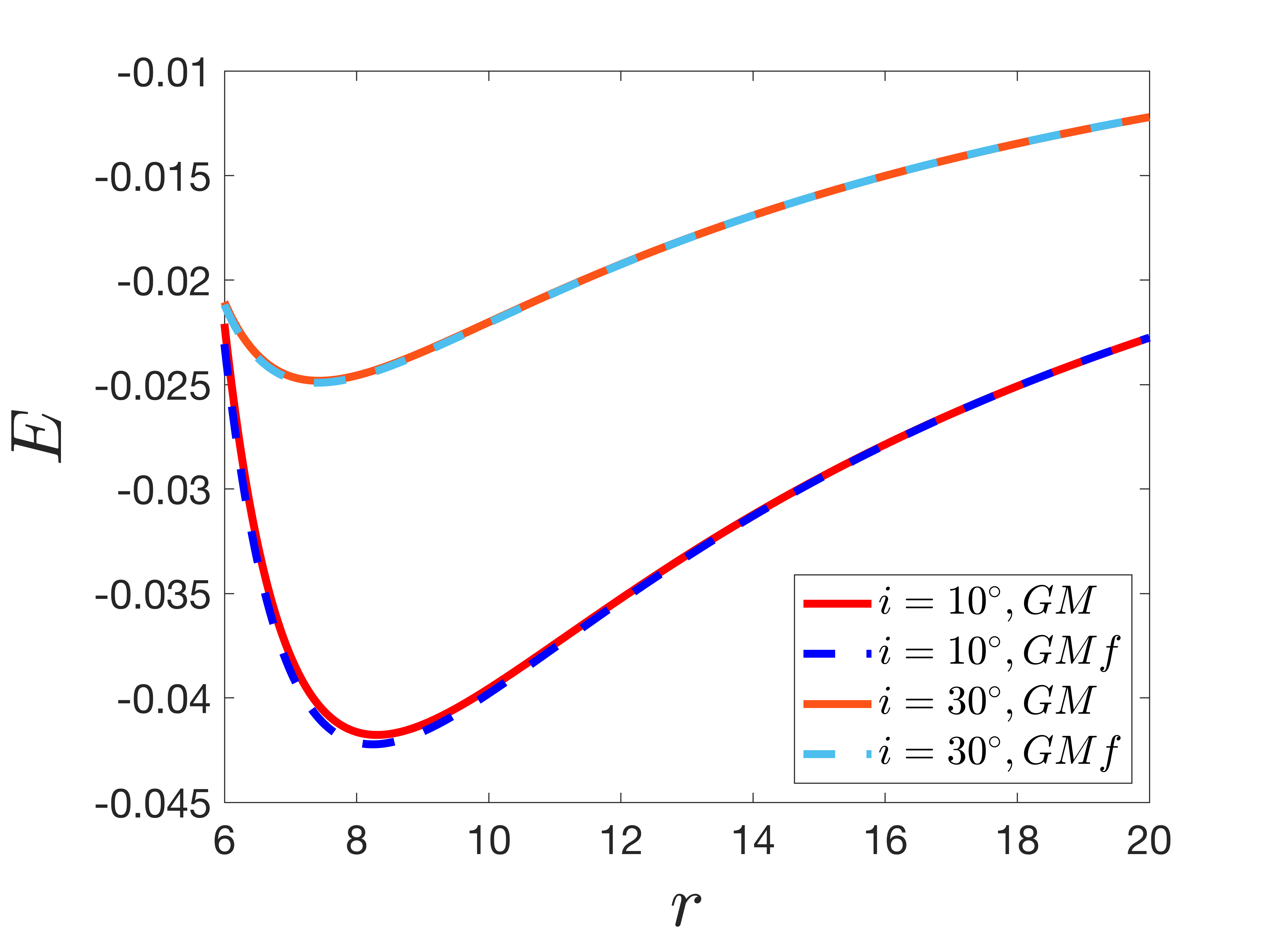
(c) Specific energy curves for $a=-0.8$, $i=10^{\circ},30^{\circ}$

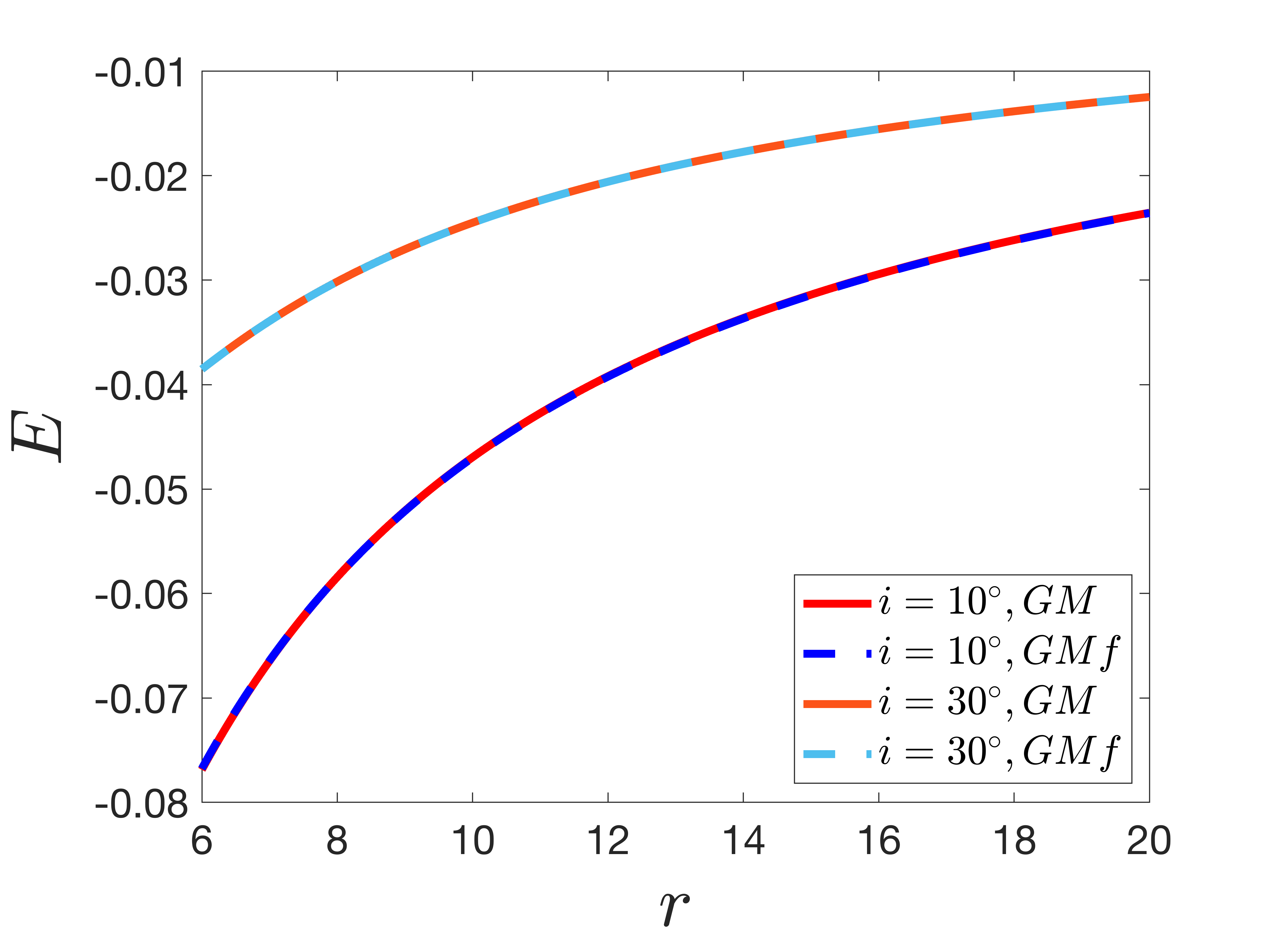
(d) Specific energy curves for $a=0.8$, $i=10^{\circ},30^{\circ}$

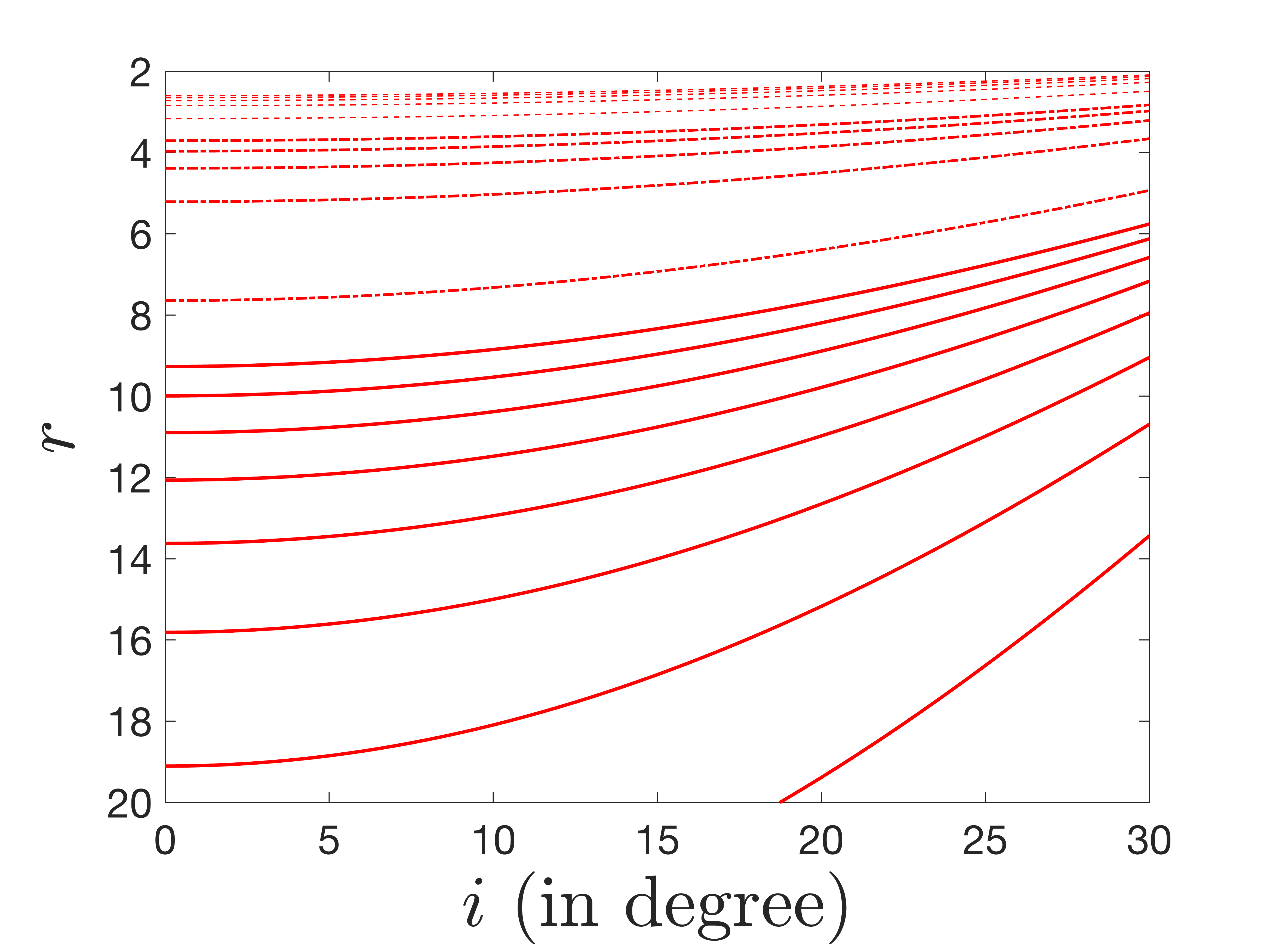
(e) Contours of constant potentials $V_{\text{GM}}$ for $a=-0.8$

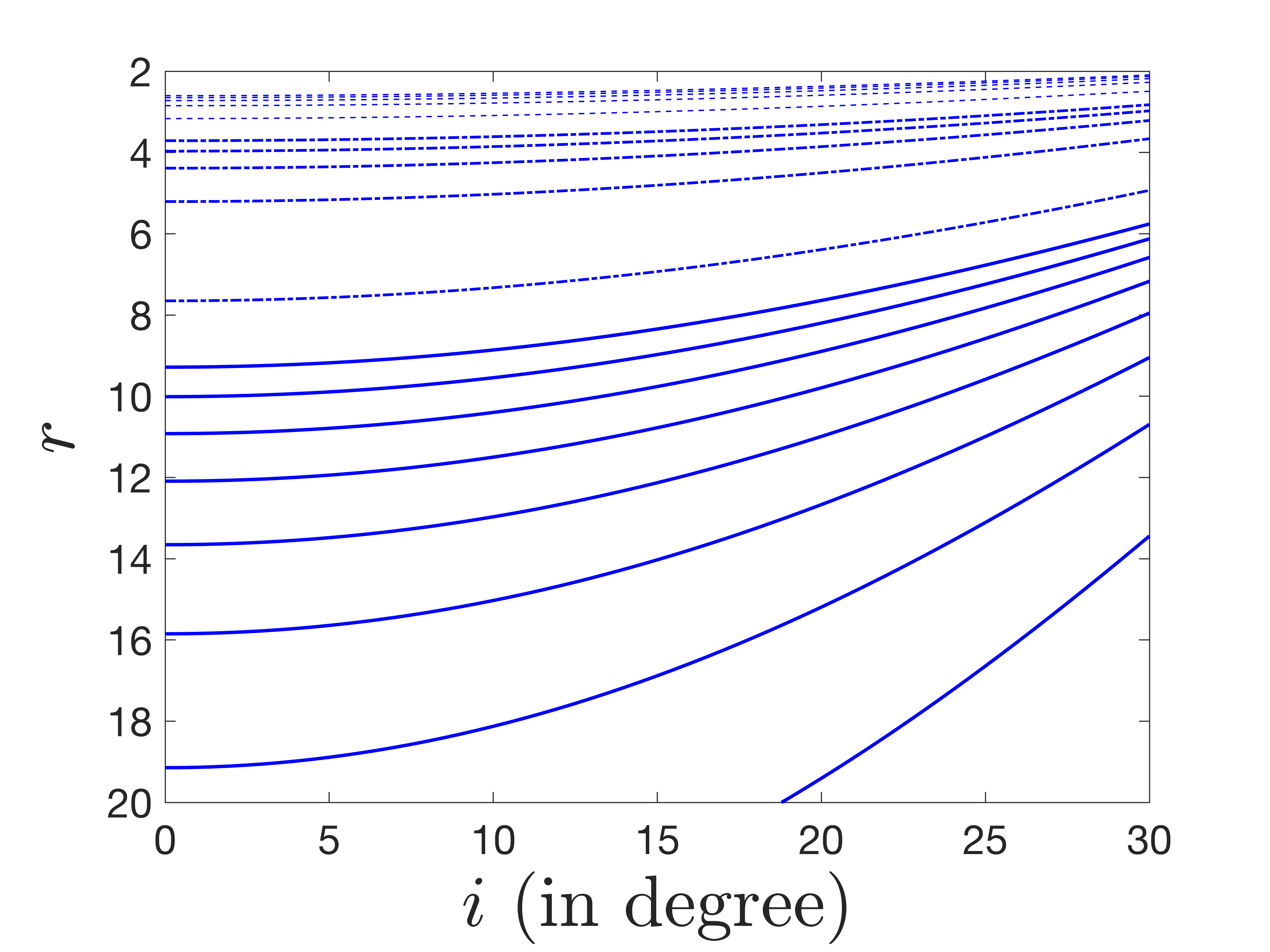
(f) Contours of constant potentials $V_{\text{GMf}}$ for $a=-0.8$

Figure 5: Comparison between GM PNP and GMf PNP. (a),(b) Fitting the GM PNP $V_{\text{GM}}$ with the GMf PNP $V_{\text{GMf}}$; (c),(d) Variation of the specific energy of circular orbits with the radial distance $r$ for $a=\pm 0.8$ and different inclination angles for both GM PNP and GMf PNP; (e),(f) Contours of constant potentials with GM PNP and GMf PNP for $a=-0.8$, consisting of solid lines corresponding to $V_{\text{PNP}}=0.045,0.06,0.075,...,0.15$, dot-dashed lines to $V_{\text{PNP}}=0.2,0.4,0.6...,1$, and dashed lines to $V_{\text{PNP}}=2,4,6,...,10$.

We can verify the quality of fitting of GMf PNP with GM PNP by doing some comparisons between them, or the derived quantities from both of them (Figure 5). In Figure 5(a) and 5(b), we show how GMf PNP fits with GM PNP for $a=\pm 0.8$ and $i=20^{\circ}$. For convenience, we have shown fewer points of GM PNP in the figures. Otherwise, we use a large number of points for efficient fitting while performing actual calculations. In Figure 5(c) and 5(d), we look for the variation in specific energy as a function of the radial distance $r$, given by the relation

$$E=\frac{r}{2}\frac{dV_{\text{PNP}}}{dr}+V_{\text{PNP}}$$ (24)

for the circular orbits governed by GM PNP and GMf PNP. We compare the results for several values of $a$ and $i$, some of which are presented here in these figures. We also compare the contours of constant potential values for GM PNP and GMf PNP with $a=-0.8$, shown in Figure 5(e) and 5(f) respectively. The studies are similar and at par with those performed in [2]. The minute differences between the two PNP s in these studies establish the quality of fitting and the effectiveness of the fitting function.

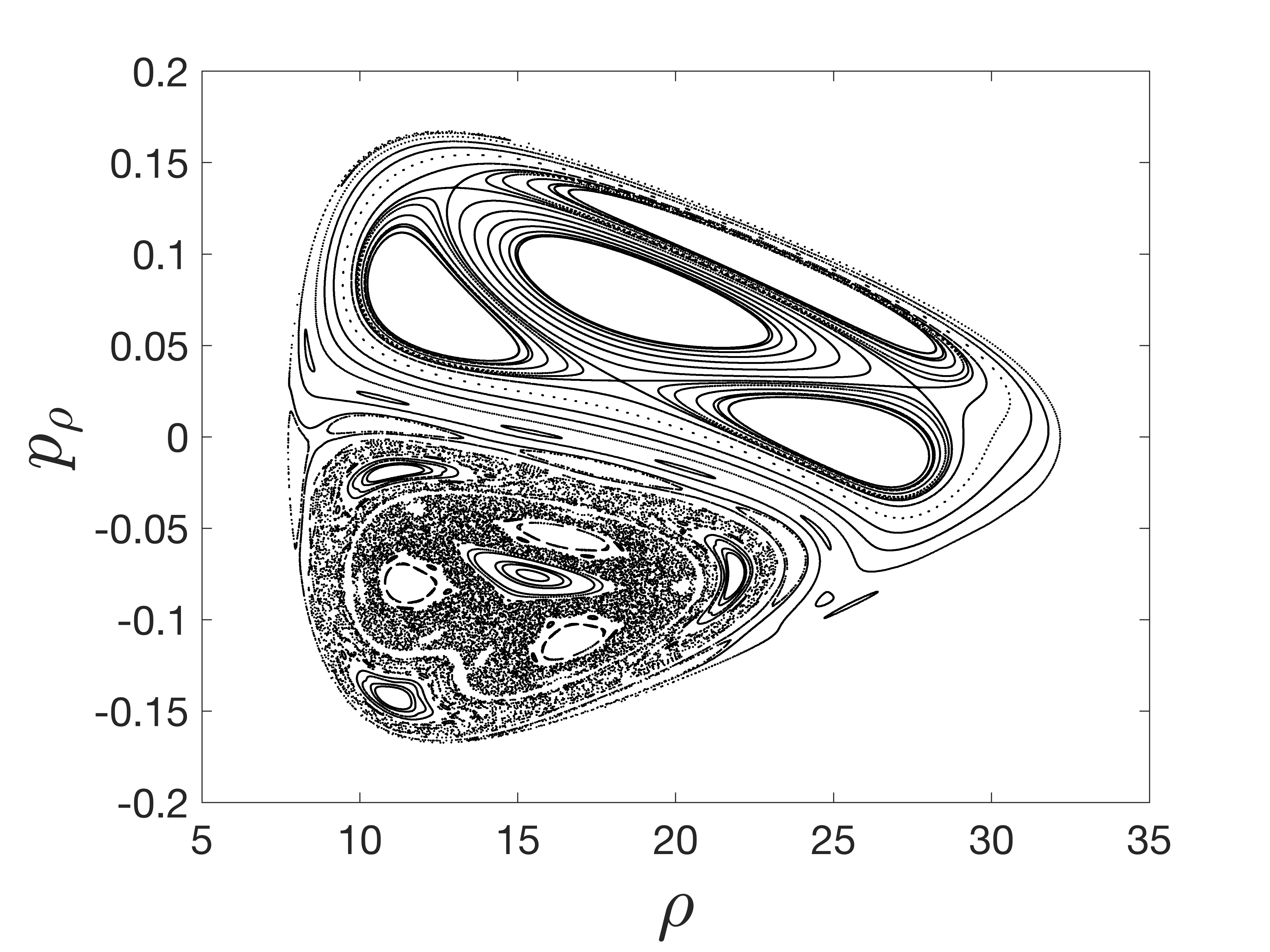
(a) $a=0.2$, GMf PNP, Non-relativistic

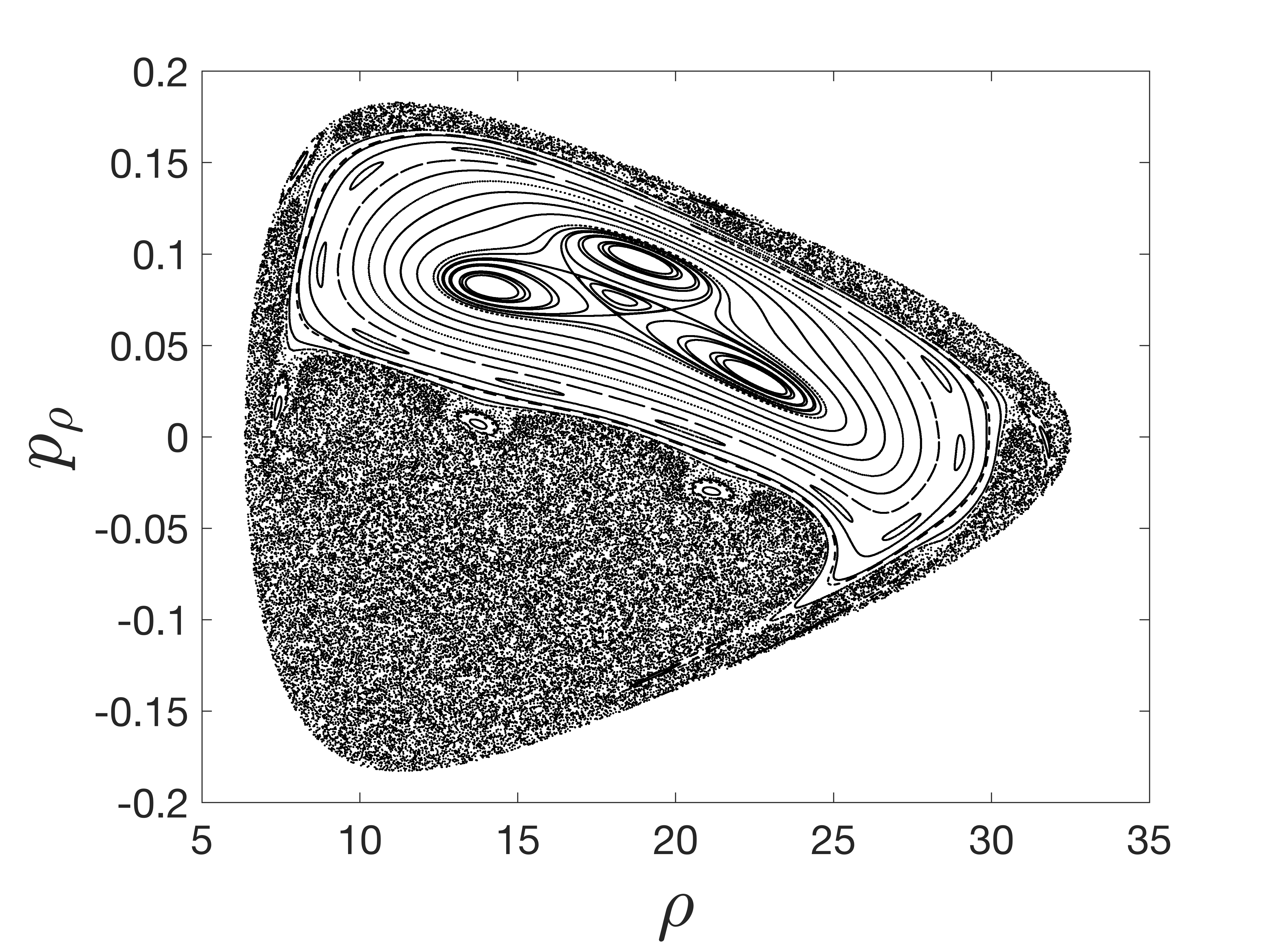
(b) $a=-0.2$, GMf PNP, Non-relativistic

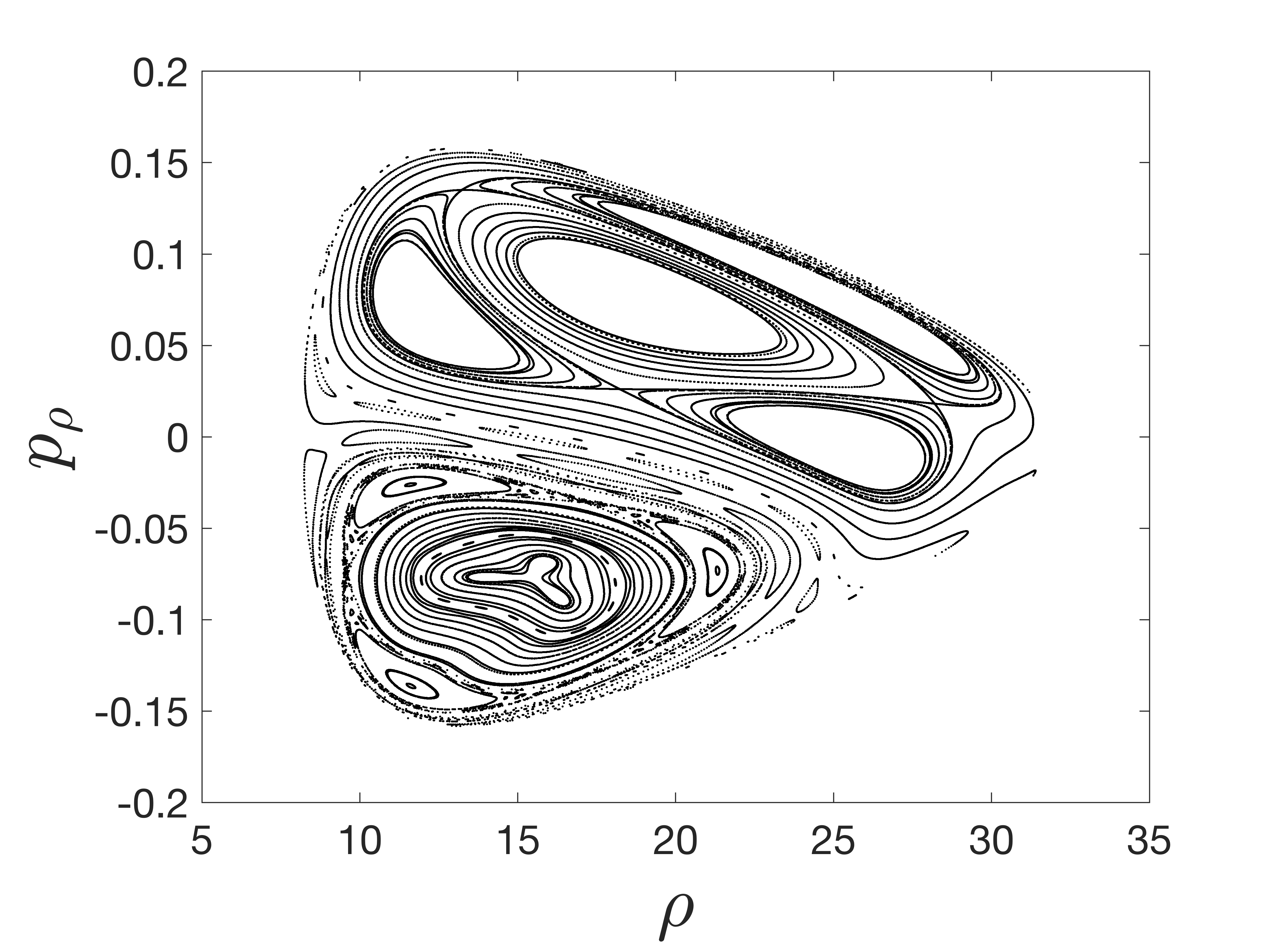
(c) $a=0.2$, ABN PNP, Non-relativistic

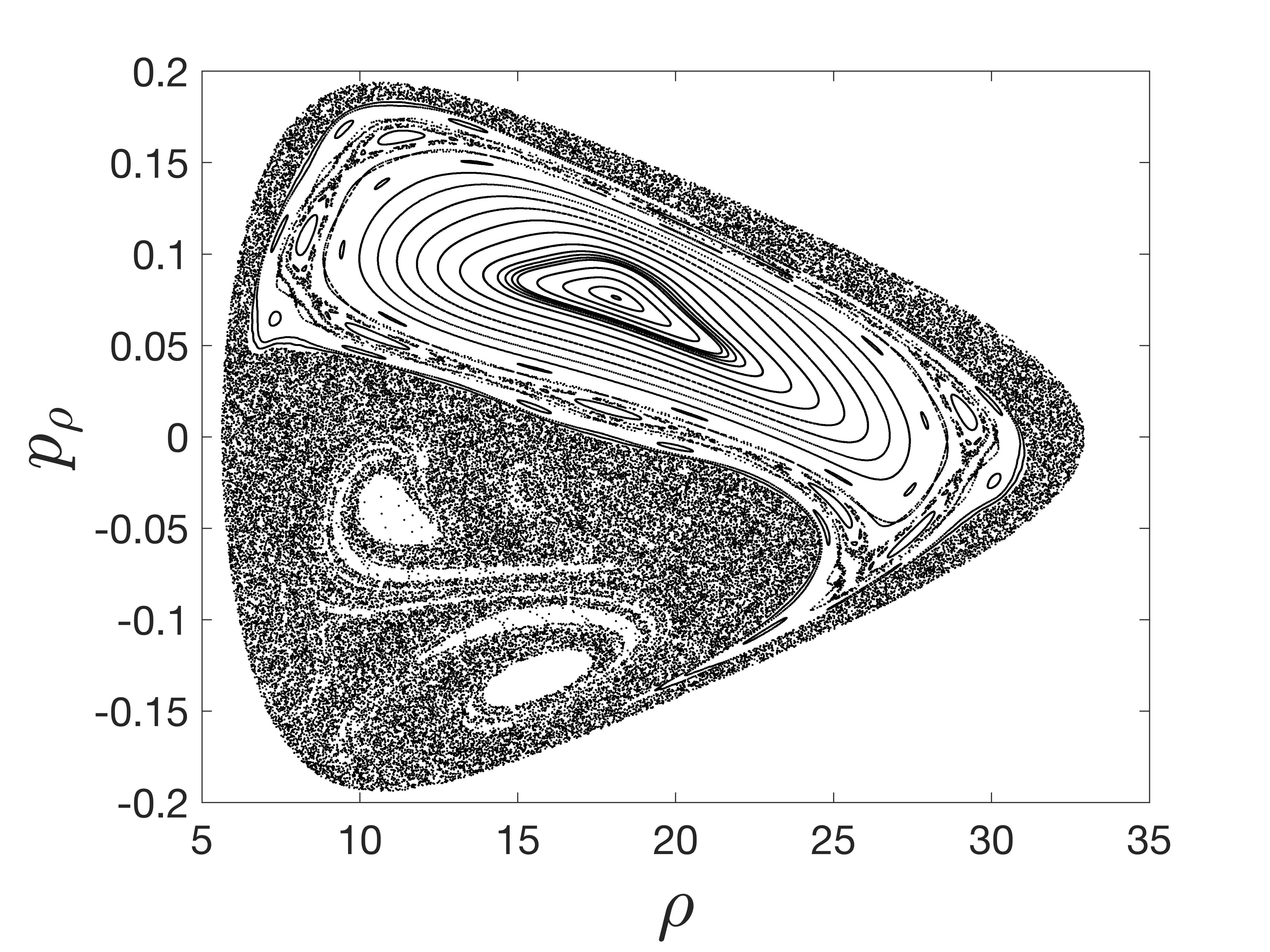
(d) $a=-0.2$, ABN PNP, Non-relativistic

Figure 6: Poincaré maps on the cross-sectional plane $z=0$ for the orbits following GMf PNP and ABN PNP with $a=\pm 0.2$, $i=0^{\circ}$, $\mathcal{D}=3\times 10^{-4}$, $E=0.975$, and $L=4.16$. The plots are evaluated without considering any special relativistic corrections.

We have already compared the effective potentials consisting of the GMf PNP with that of the ABN PNP in section 2.3. Now, we must compare the Poincaré Maps generated using the two potentials (Figure 6). Apparently, we are considering the orbits on the equatorial plane in this case ($i=0^{\circ}$). We can observe the usual frame-dragging effect for GMf PNP (Figure 6(a) and 6(b)). The chaotic nature of the orbits for $a=-0.2$ is significantly higher than that for $a=0.2$. The frame-dragging effect is also evident in the Poincaré Maps corresponding to the orbits derived from ABN PNP (Figure 6(c) and 6(d)). The number of regular orbits has decreased significantly in the map for $a=-0.2$ compared to that for $a=0.2$. However, it is to be noted that the degree of chaos in the map for $a=0.2$ evaluated from GMf PNP (Figure 6(a)) is more than that derived from ABN PNP (Figure 6(c)). On the contrary, the chaotic nature of the orbits in the map for $a=-0.2$ evaluated from GMf PNP (Figure 6(b)) is less compared to that derived from ABN PNP (Figure 6(d)). This is the consequence of the result that we presented in section 2.3, where we made a comparison between the two PNP s (Figure 2). The relative shift in the local minima of the effective potentials affects the chaotic behaviour of the orbits in the way we can see in Figure 6.

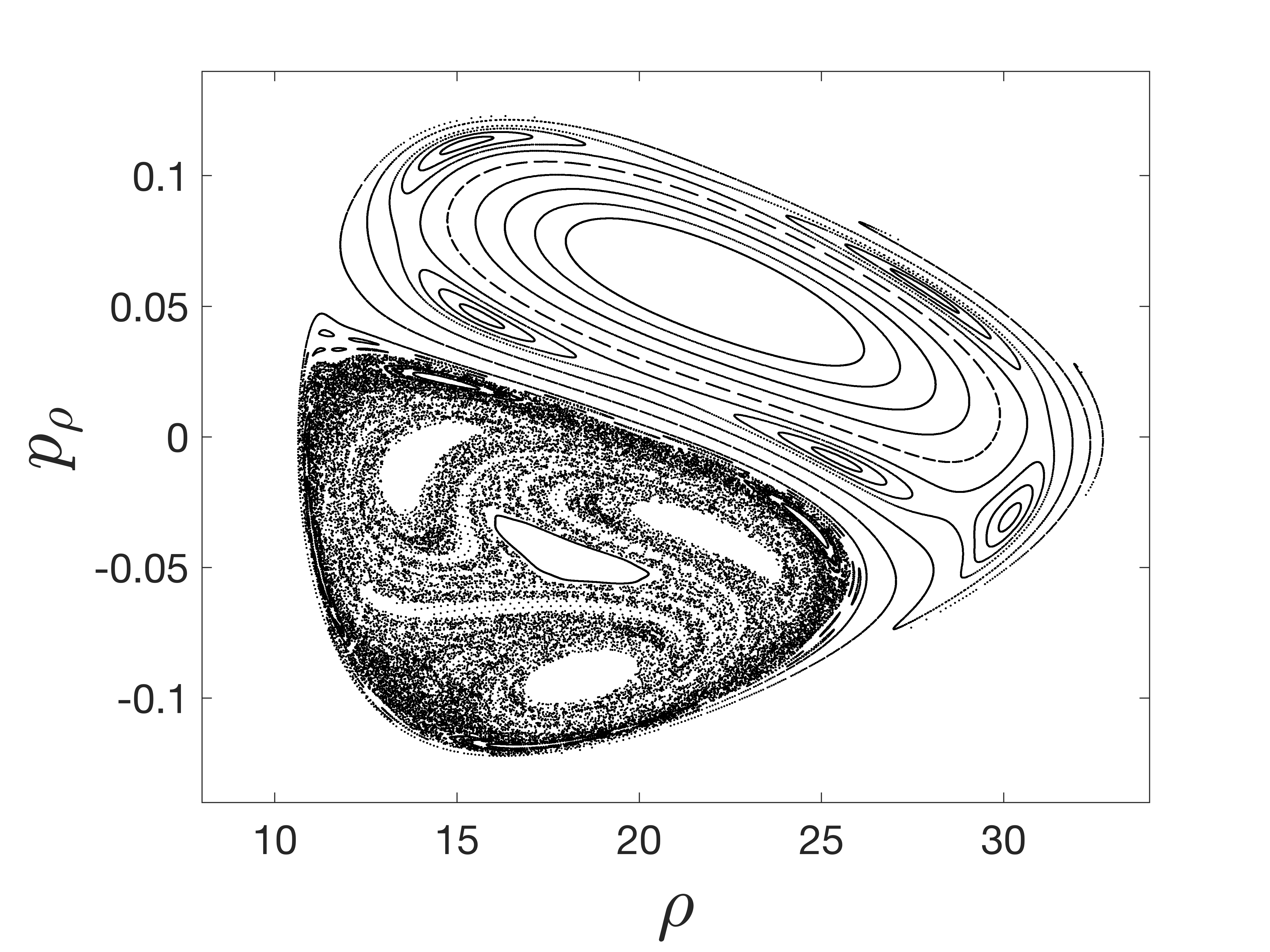
(a) $a=-0.6$, $i=10^{\circ}$, Non-relativistic

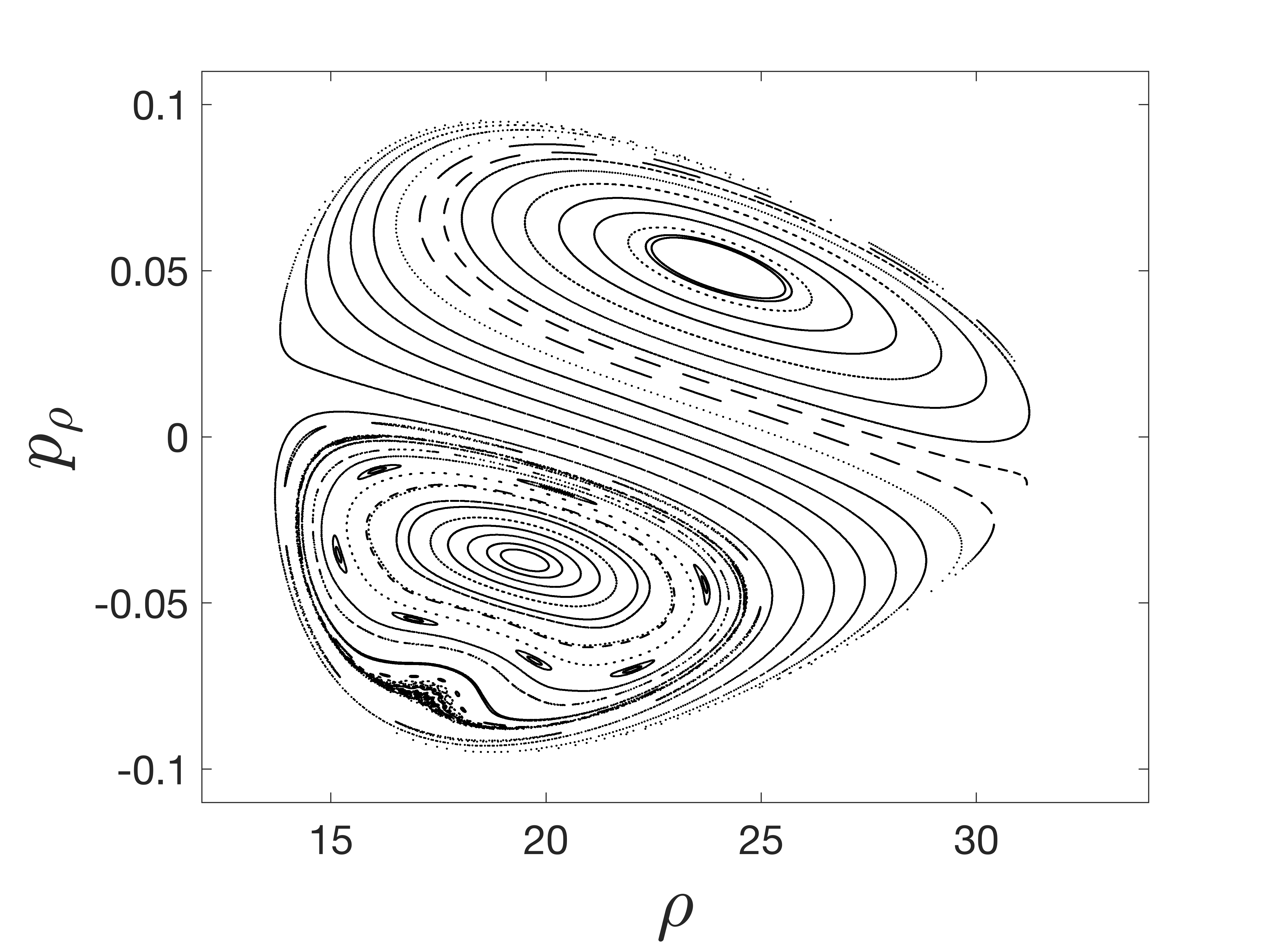
(b) $a=0.6$, $i=10^{\circ}$, Non-relativistic

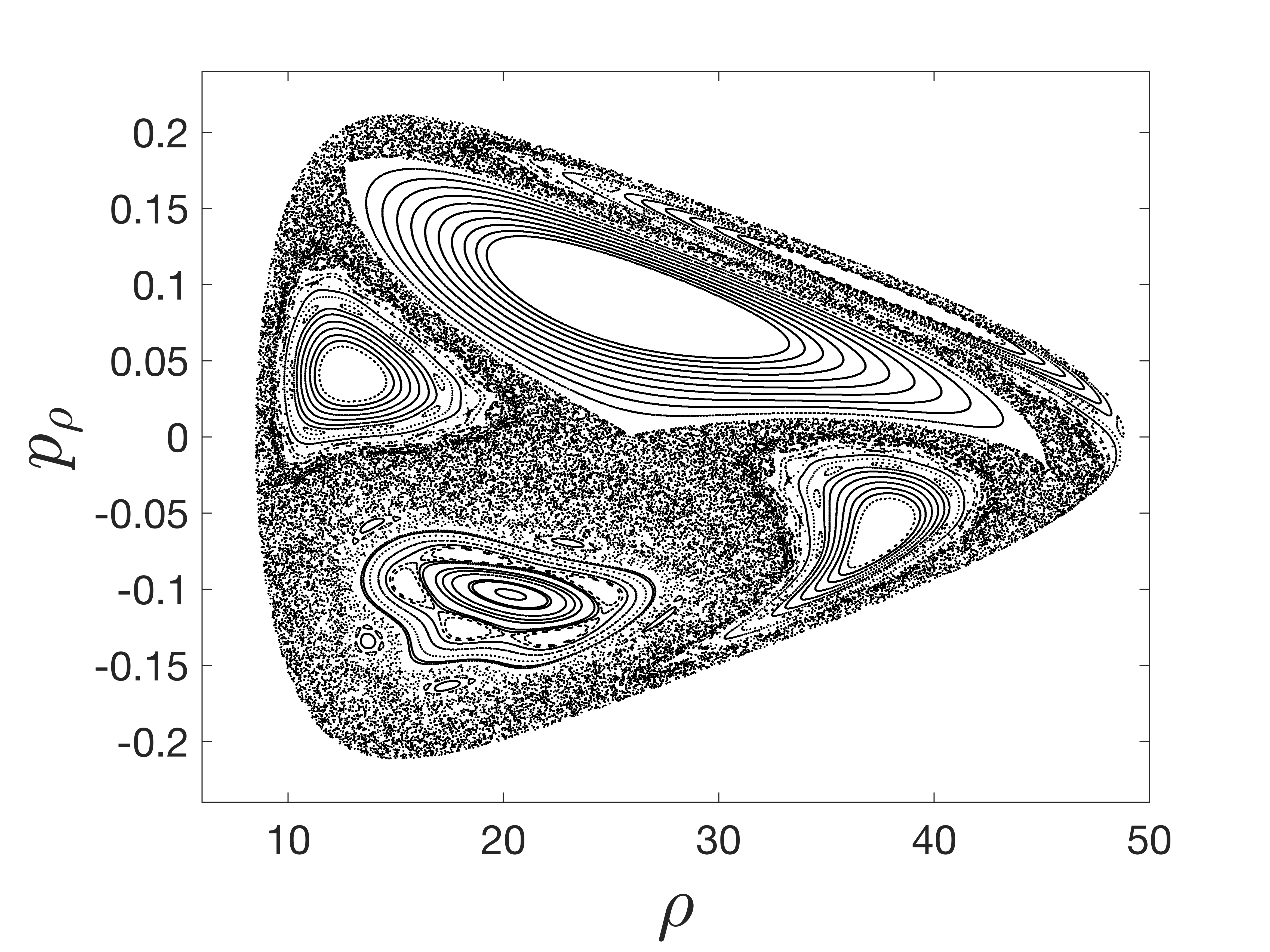
(c) $a=-0.6$, $i=25^{\circ}$, Non-relativistic

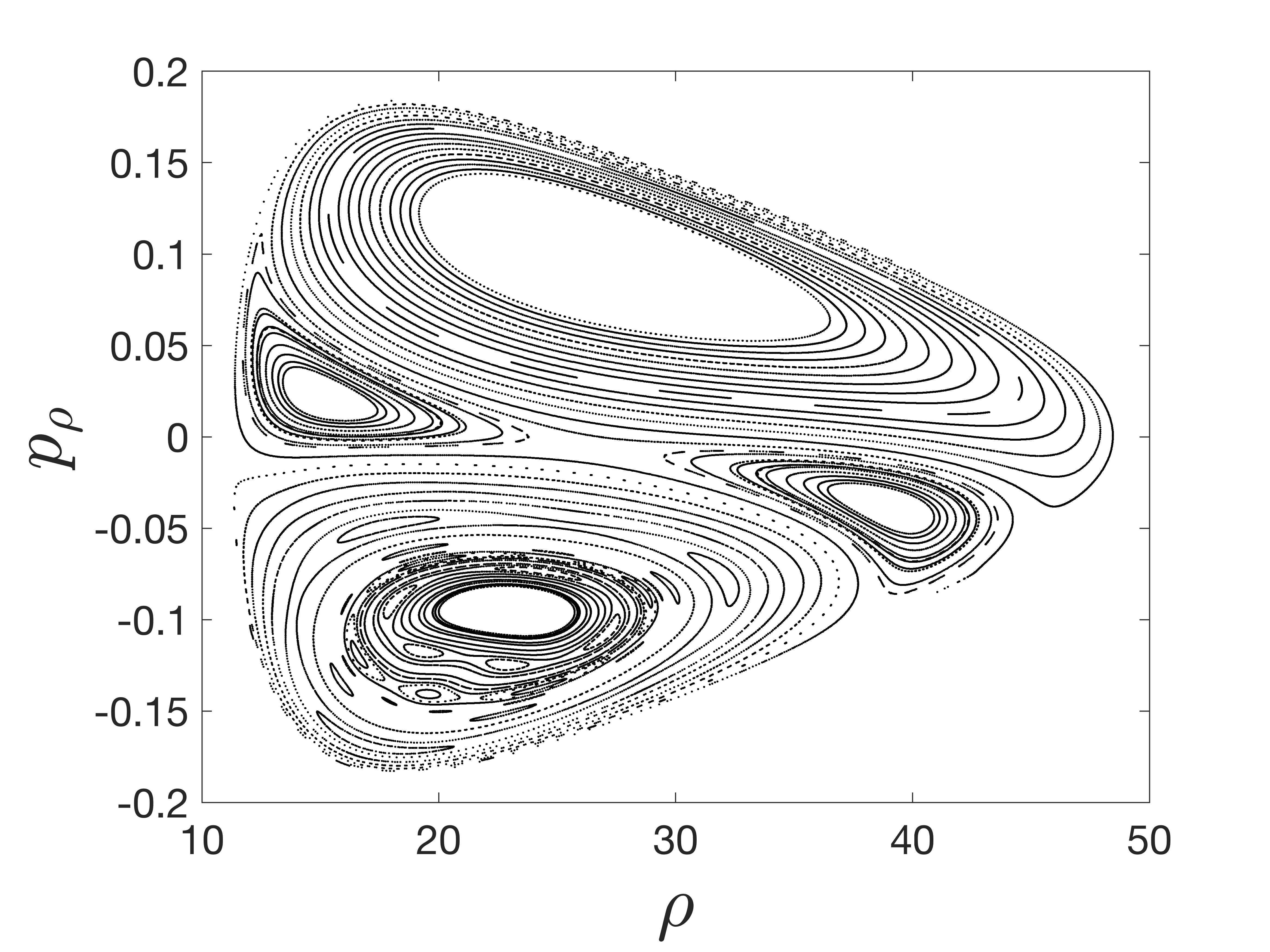
(d) $a=0.6$, $i=25^{\circ}$, Non-relativistic

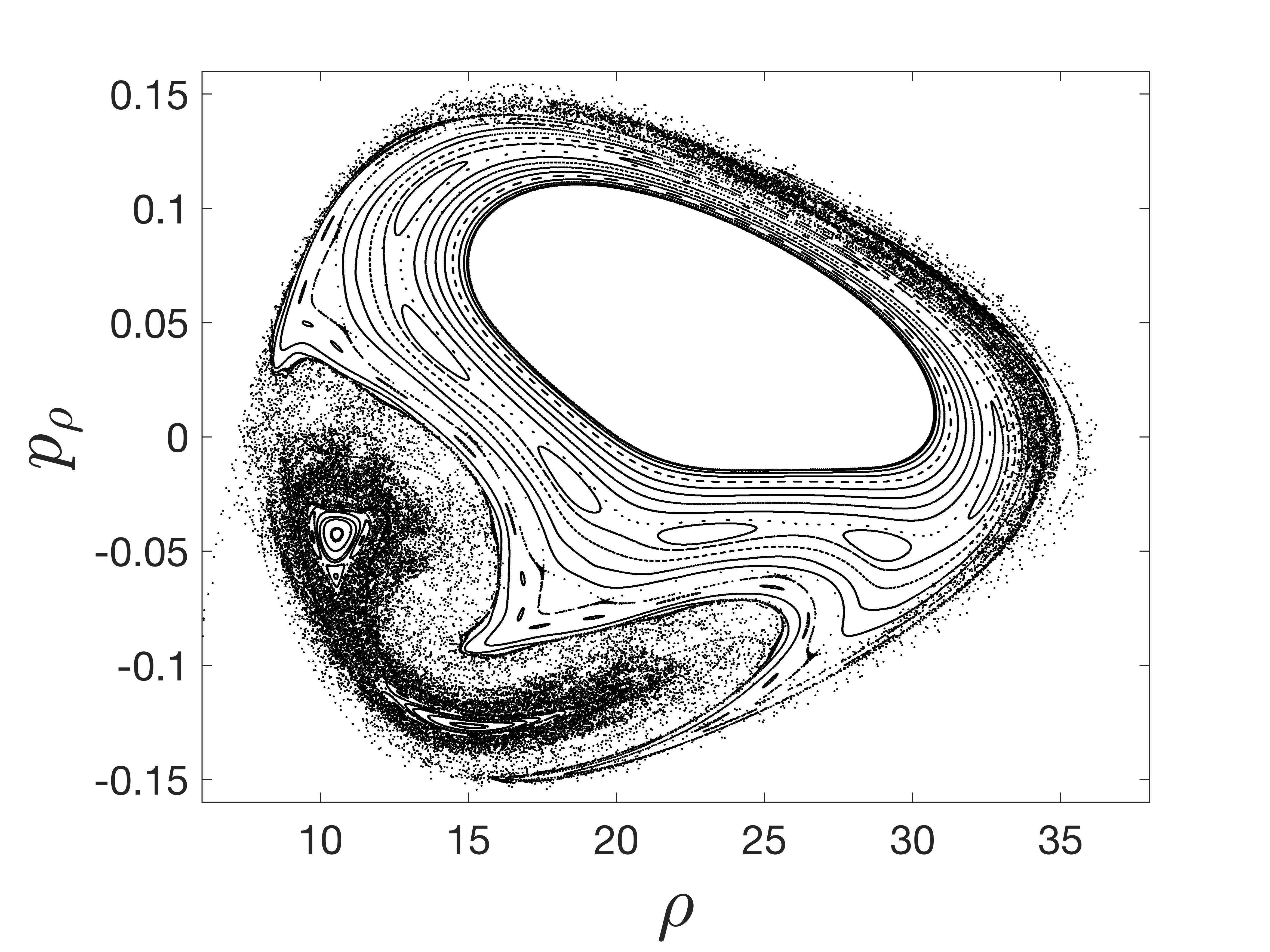
(e) $a=-0.15$, $i=25^{\circ}$, Relativistic

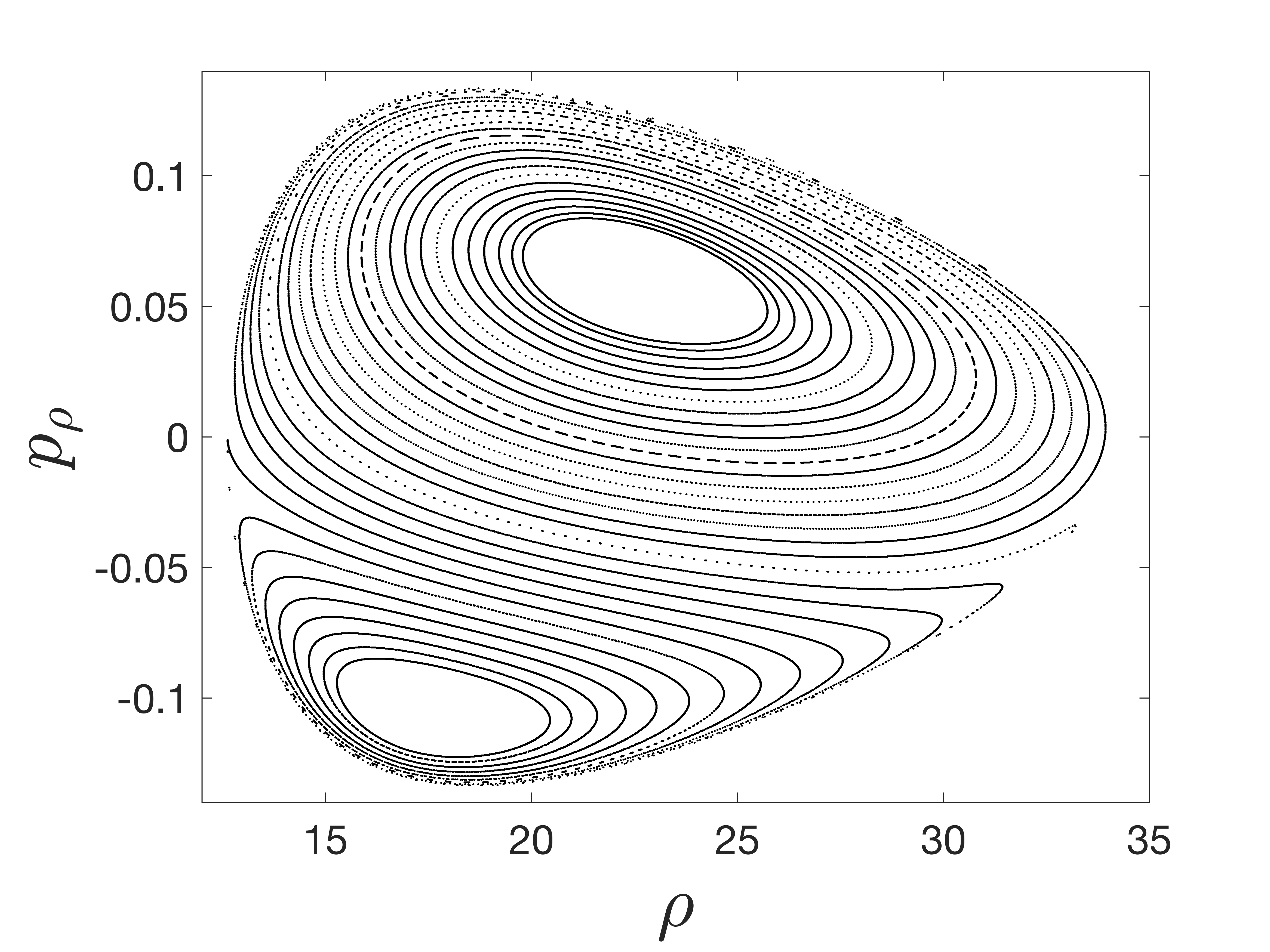
(f) $a=0.15$, $i=25^{\circ}$, Relativistic

Figure 7: Poincaré maps on the cross-sectional plane $z=0$ for the orbits governed by GMf PNP with different values of the Kerr parameter $a$, and fixed values of orbital parameters, such that (a)-(b) $i=10^{\circ}$, $E=0.976$, $L=4.90$, $\mathcal{D}=3\times 10^{-4}$, (c)-(d) $i=25^{\circ}$, $E=0.9734$, $L=5.82$, $\mathcal{D}=2\times 10^{-4}$, and (e)-(f) $i=25^{\circ}$, $E=0.965$, $L=5.835$, $\mathcal{D}=2\times 10^{-4}$.

To observe how the chaoticity of the inclined orbits changes with the rotation of the COP, we studied the chaotic nature of the orbits for the whole range of the Kerr parameter $\left(-1\leq a<1\right)$. First, we consider the orbits with a relatively smaller value of inclination ($i=10^{\circ}$), along with particular values of dipole coefficient $\mathcal{D}$, energy $E$, and angular momentum $L$. We observe that the orbits around the counter-rotating COP s (such as Figure 7(a)) are more chaotic than that around the co-rotating ones (such as Figure 7(b)). For any negative value of $a$, we have examined the Poincaré Map plot for the corresponding positive value of $a$. The former is apparently more chaotic than the latter for all the cases. This occurs because of the usual frame-dragging effect. We have studied the gradual change in the chaoticity from $a=-1$ to $a\approx+1$. The systematic suppression of chaos with respect to the Kerr parameter is evident. We can consider a higher inclination such as $i=25^{\circ}$, and look for how the chaoticity changes for different values of $a$. We get to observe a similar trend in this case as well. However, the change in chaoticity is more for the higher value of the inclination angle, when the Kerr parameter changes from $a=-0.6$ (Figure 7(c)) to $a=0.6$ (Figure 7(d)). For the relativistic test particle, the region of chaos decreases significantly when the Kerr parameter changes from $a=-0.15$ (Figure 7(e)) to $a=0.15$ (Figure 7(f)). From this, we can say that the degree of chaos has a negative correlation with the Kerr parameter $a$ for any given inclination angle. However, quantitative analysis in section 4 will reveal more details and intricacies, where a significantly larger number of initial conditions can be considered and examined for the entire range of $a$.

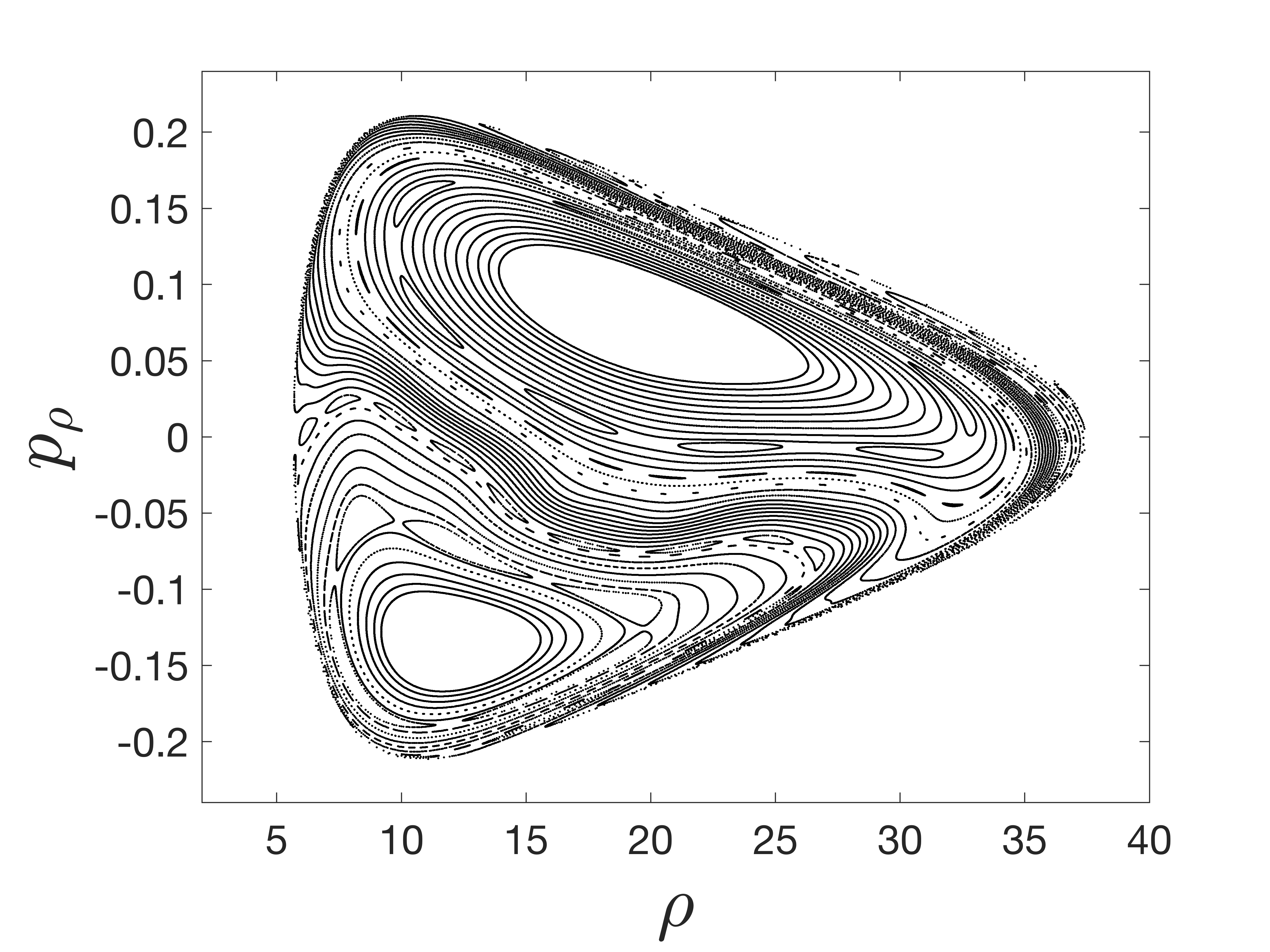
(a) $i=10^{\circ}$, $a=-0.15$, Non-relativistic

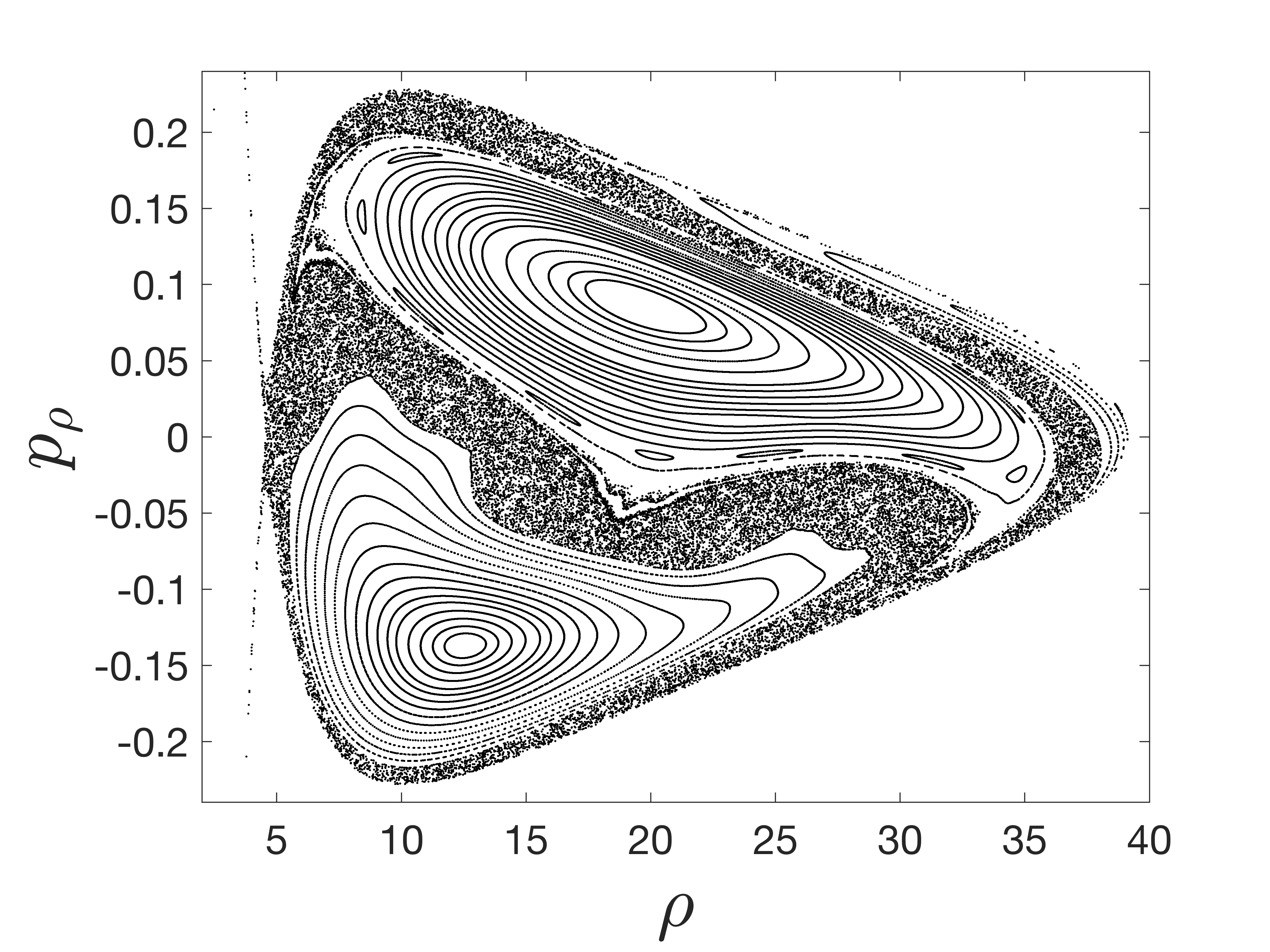
(b) $i=12^{\circ}$, $a=-0.15$, Non-relativistic

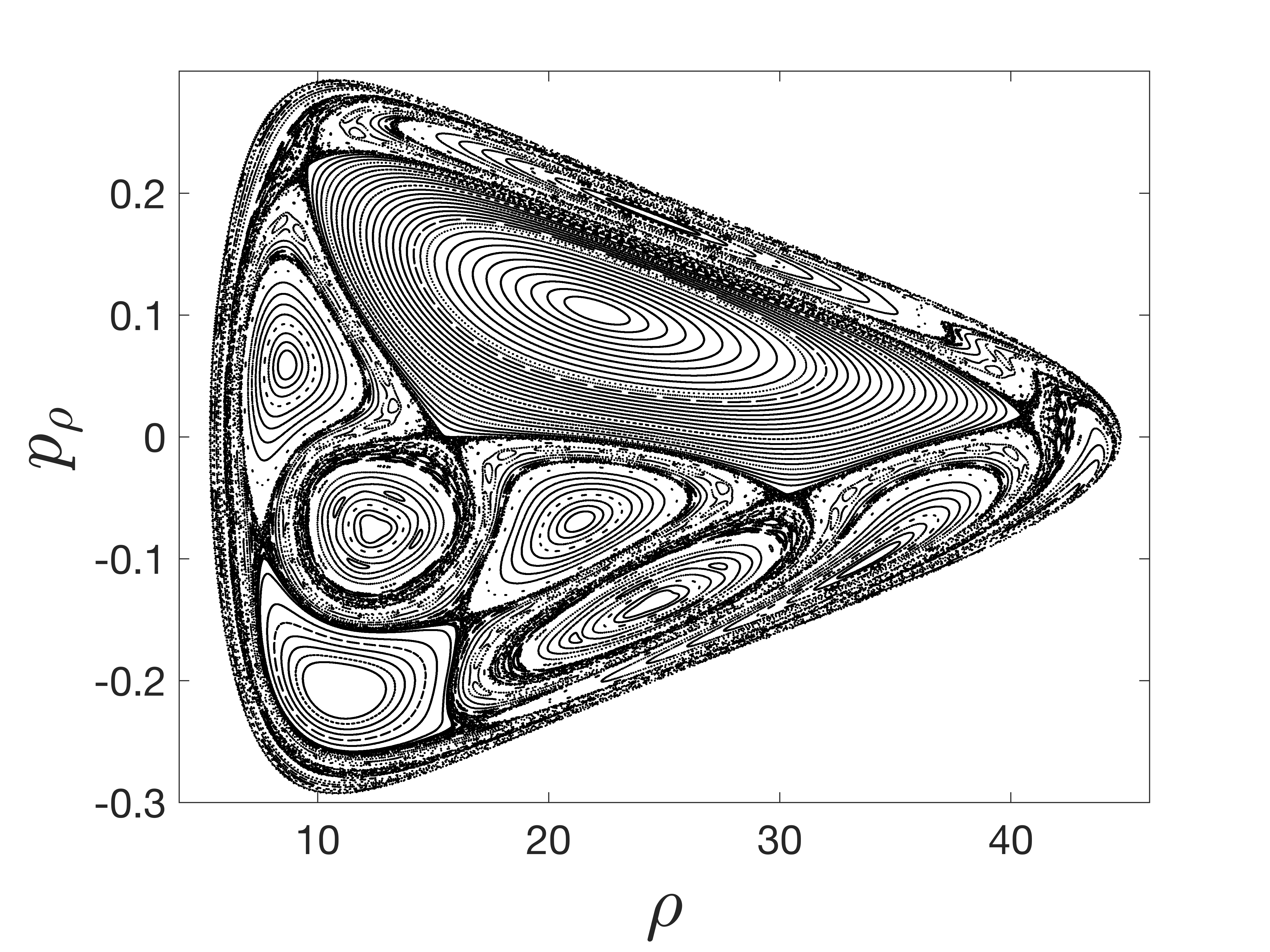
(c) $i=28^{\circ}$, $a=-0.15$, Non-relativistic

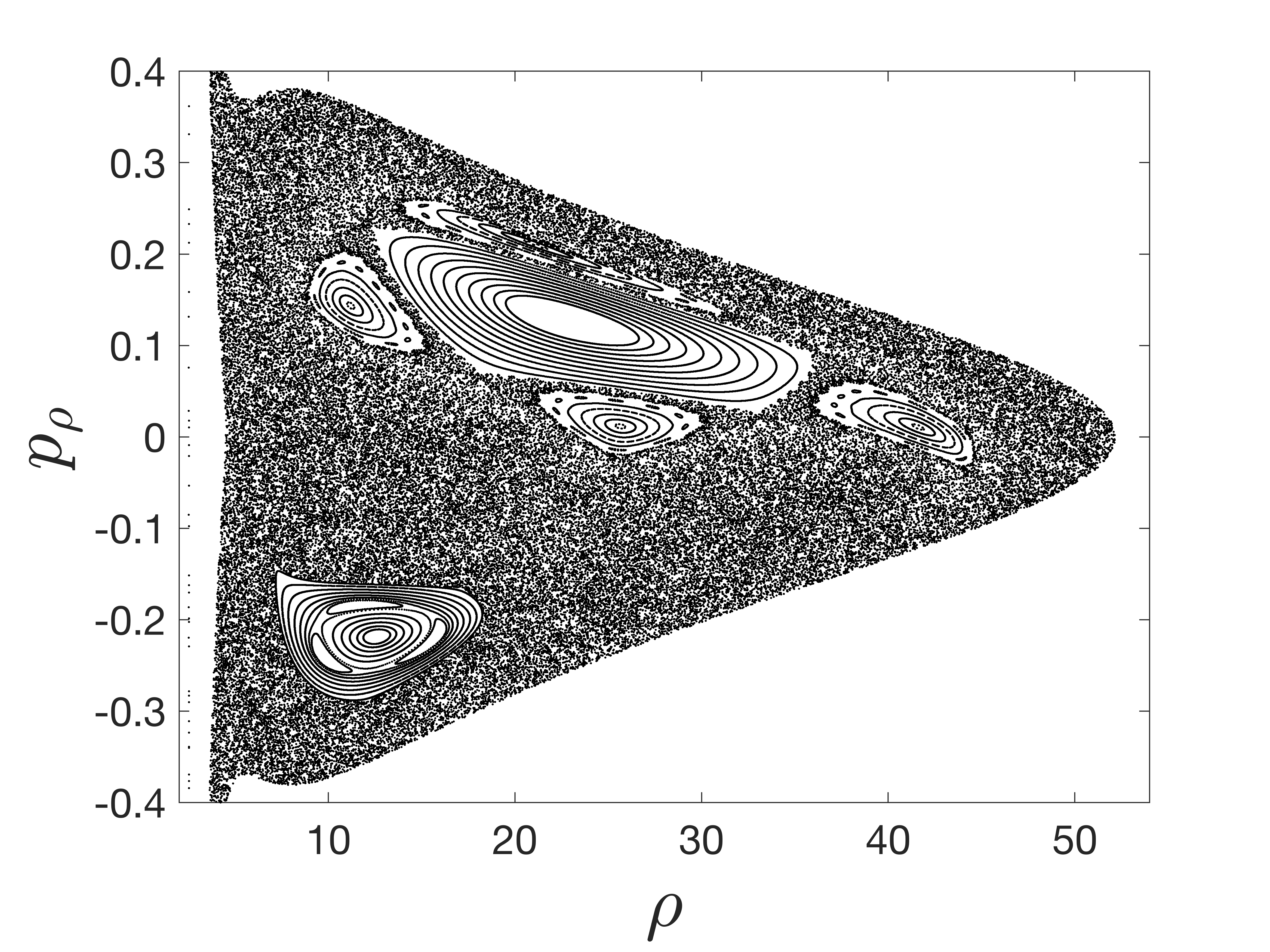
(d) $i=30^{\circ}$, $a=-0.15$, Non-relativistic

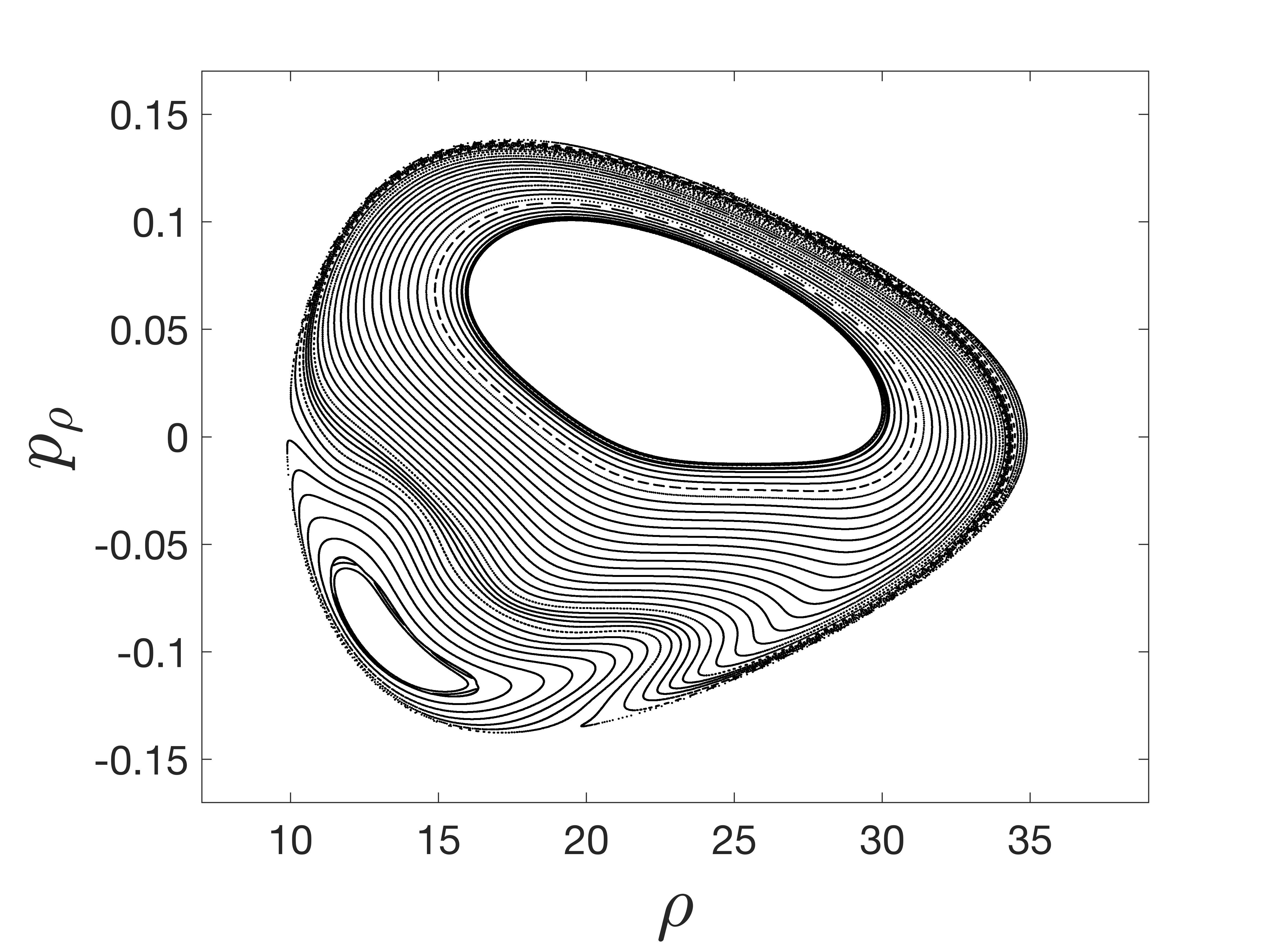
(e) $i=25^{\circ}$, $a=-0.15$, Relativistic

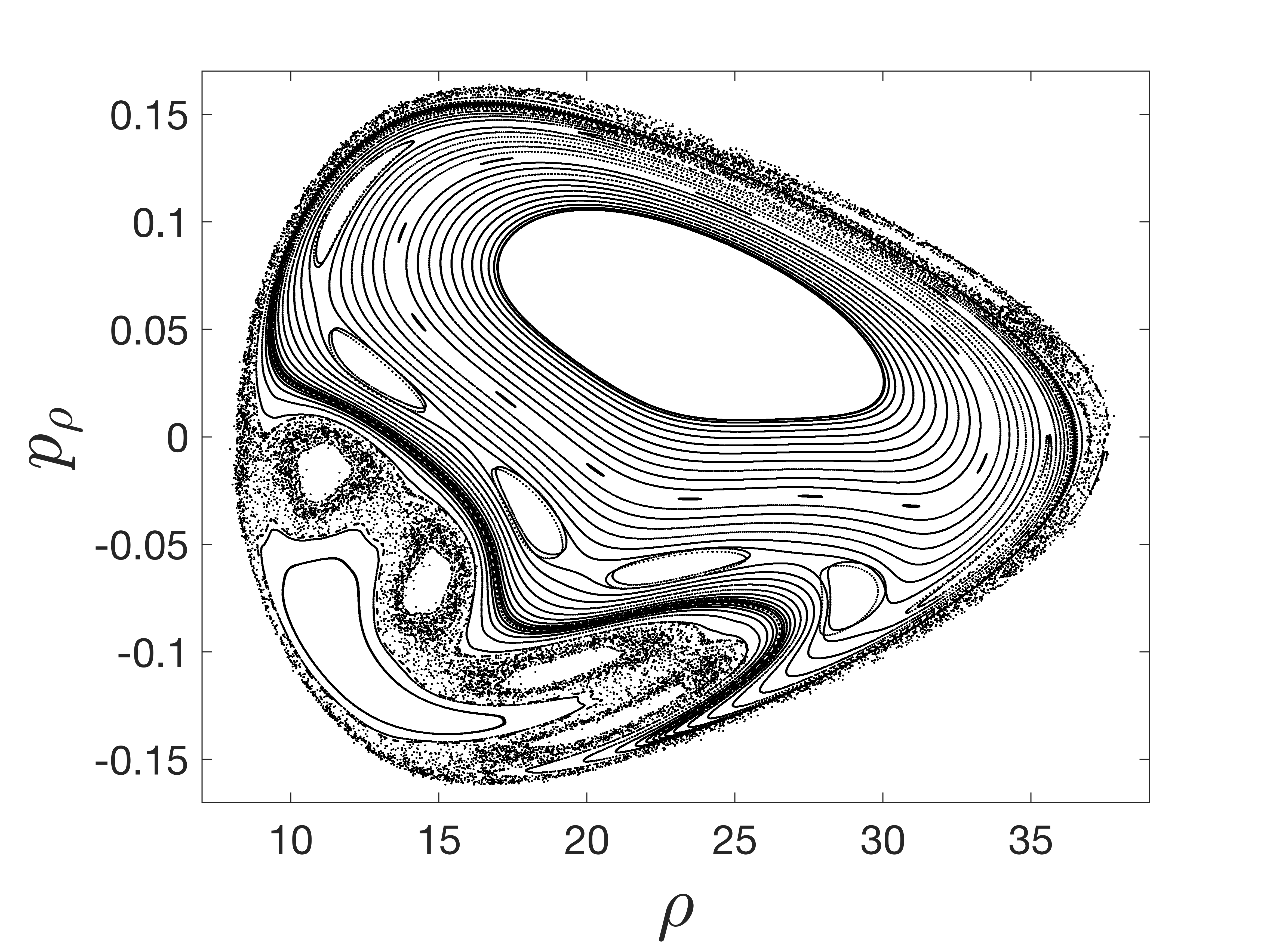
(f) $i=26^{\circ}$, $a=-0.15$, Relativistic

Figure 8: Poincaré maps on the cross-sectional plane $z=0$ for the orbits governed by GMf PNP with different values of the inclination angle $i$, and fixed values of orbital parameters, such that (a)-(b) $a=-0.15$, $E=0.976$, $L=4.22$, $\mathcal{D}=2\times 10^{-4}$, (c)-(d) $a=-0.15$, $E=0.965$, $L=5.48$, $\mathcal{D}=2\times 10^{-4}$, and (e)-(f) $a=-0.15$, $E=0.965$, $L=5.95$, $\mathcal{D}=2\times 10^{-4}$.

After finding out the dependence of chaos on the Kerr parameter $a$, we studied the change in the chaotic nature of the orbits with respect to the inclination angle $i$ for both non-relativistic and relativistic particles (Figure 8). In all cases, the chaotic behaviour of the orbits increases with the angle of inclination $i$. For the non-relativistic orbits with higher inclinations, the Poincaré Maps change drastically when the inclination angle increases from $i=28^{\circ}$ (Figure 8(c)) to $i=30^{\circ}$ (Figure 8(d)). In comparison to this, the change in the nature of orbits for smaller inclination angles is more gradual. A smaller region of order converts into the region of chaos when the inclination angle increases from $i=10^{\circ}$ (Figure 8(a)) to $i=12^{\circ}$ (Figure 8(b)). We have already observed the change to be gradual at smaller inclination angles in Figure 4 when we studied the Poincaré Maps corresponding to the off-equatorial orbits around the Schwarzschild-like COP s. This phenomenon will also be corroborated and studied in detail using the quantitative analysis of chaos in the next section. Similar to the non-relativistic case, the chaotic nature of the relativistic orbits has a positive correlation with the inclination angle $i$. The Poincaré Map plot for $i=25^{\circ}$ (Figure 8(e)) consists of regular orbits, many of which extinguish and turn into chaotic orbits when the inclination angle increases to $i=26^{\circ}$ (Figure 8(f)).

4 Quantification of chaos using Maximum Lyapunov Exponents

As we have studied the chaotic dynamics of the orbits qualitatively, we proceed to look for a quantitative way of studying chaos. There are many chaotic indicators available in the literature. We have used the Lyapunov Exponent in this regard as it is easy to implement, can efficiently distinguish between order and chaos in our system, and is very effective in studying the chaotic correlations over a long range of dynamical parameters. One can measure the exponential divergence of two neighbouring orbits while their starting point is very close to each other [68]. The number of exponents will equal the number of dimensions of the phase space. However, in the long run (for $t\rightarrow\infty$), the maximum of the exponents dominates. This is known as the MLE [4, 8]. This can be calculated as

$$\Lambda_{\text{max}}=\lim\limits_{\begin{subarray}{c}t\to\infty\\ ||\delta x(0)||\to 0\end{subarray}}\left(\frac{1}{t}\ln\frac{||\delta x(t)||}{||\delta x(0)||}\right)$$ (25)

where $||\delta x(t)||$ is the norm of the deviation between the two neighbouring orbits in the phase space at time $t$. It can be evaluated using the Difference-Hamiltonian and the variational equations [69]. This method is known as the variational method. Although the method is very accurate, the calculation is intensively rigorous with the mathematically complex form of GMf PNP. As an alternative, we have used the two-particle method, a more convenient and less rigorous way of calculating MLE s [8].

To achieve accurate results using the two-particle method, the initial deviation has to be very small, and the precision of the computational instrument has to be high. Furthermore, we need to re-normalise the deviated orbit after every time step $\tau$ using the Gram-Schmidt renormalisation scheme [70] so that the MLE s do not diverge very quickly. For a particular set of parameters, we can consider a large number of initial conditions evenly distributed over the allowable phase space and calculate MLE s for each of them. Thereafter, we can take the average of all the exponents $\left(\Lambda_{\text{av}}\right)$ and consider this as a rough quantitative measure of the overall chaos in the system. In the present work, we have used double precision for the computation of the MLE s. For each initial condition, the initial deviation has been taken to be $\delta x(0)=10^{-8}$, and the calculation has been carried out for $n=10^{5}$ iterations with renormalisation time-step $\tau=0.1$. The threshold has been found to be $\approx 1.5\times 10^{-4}$, which means the value of $\Lambda_{\text{max}}$ is smaller than $1.5\times 10^{-4}$ for regular orbits and it is more than $1.5\times 10^{-4}$ for chaotic orbits.

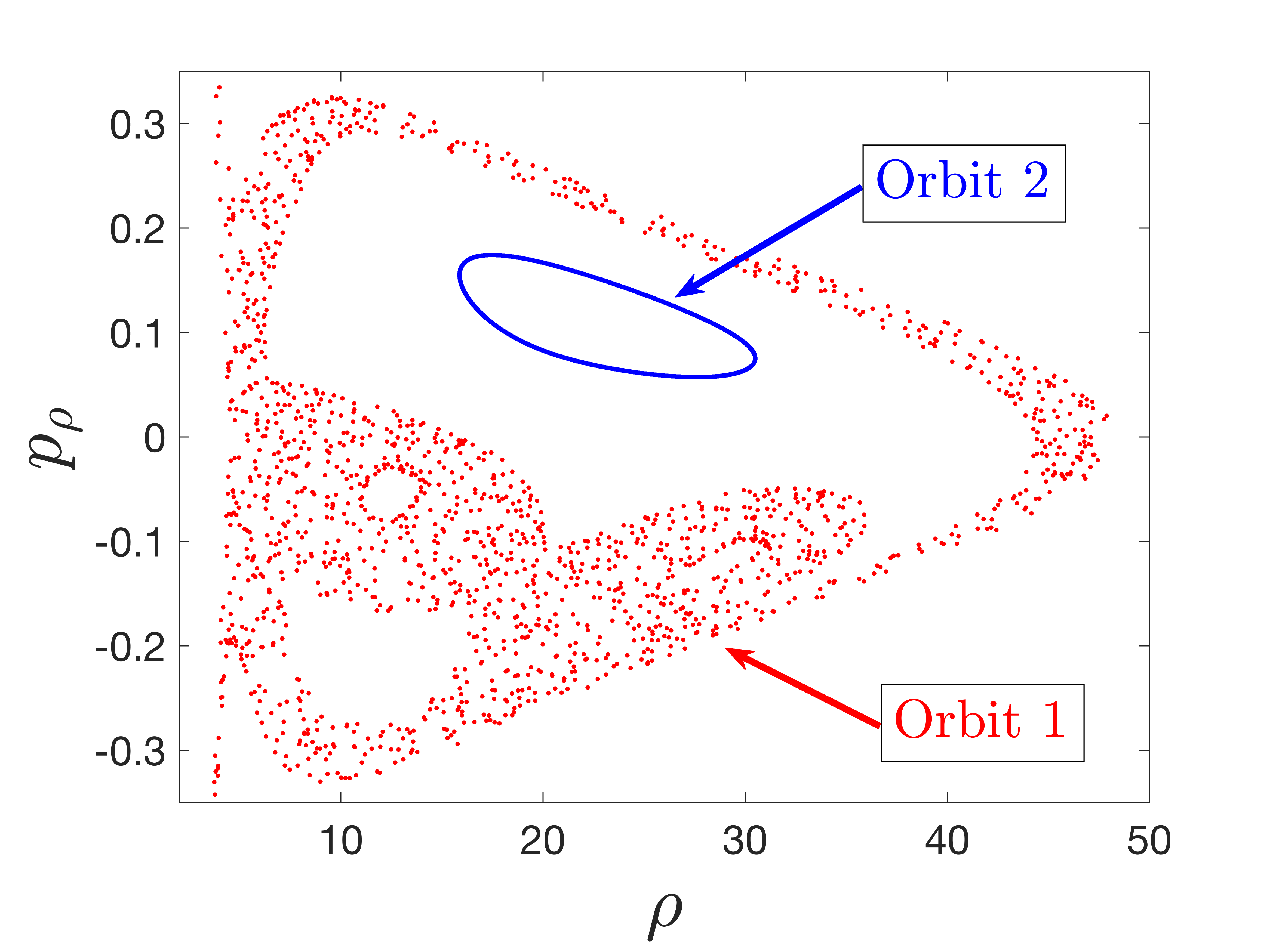
(a) Poincaré sections for orbit 1 (chaotic) and orbit 2 (regular)

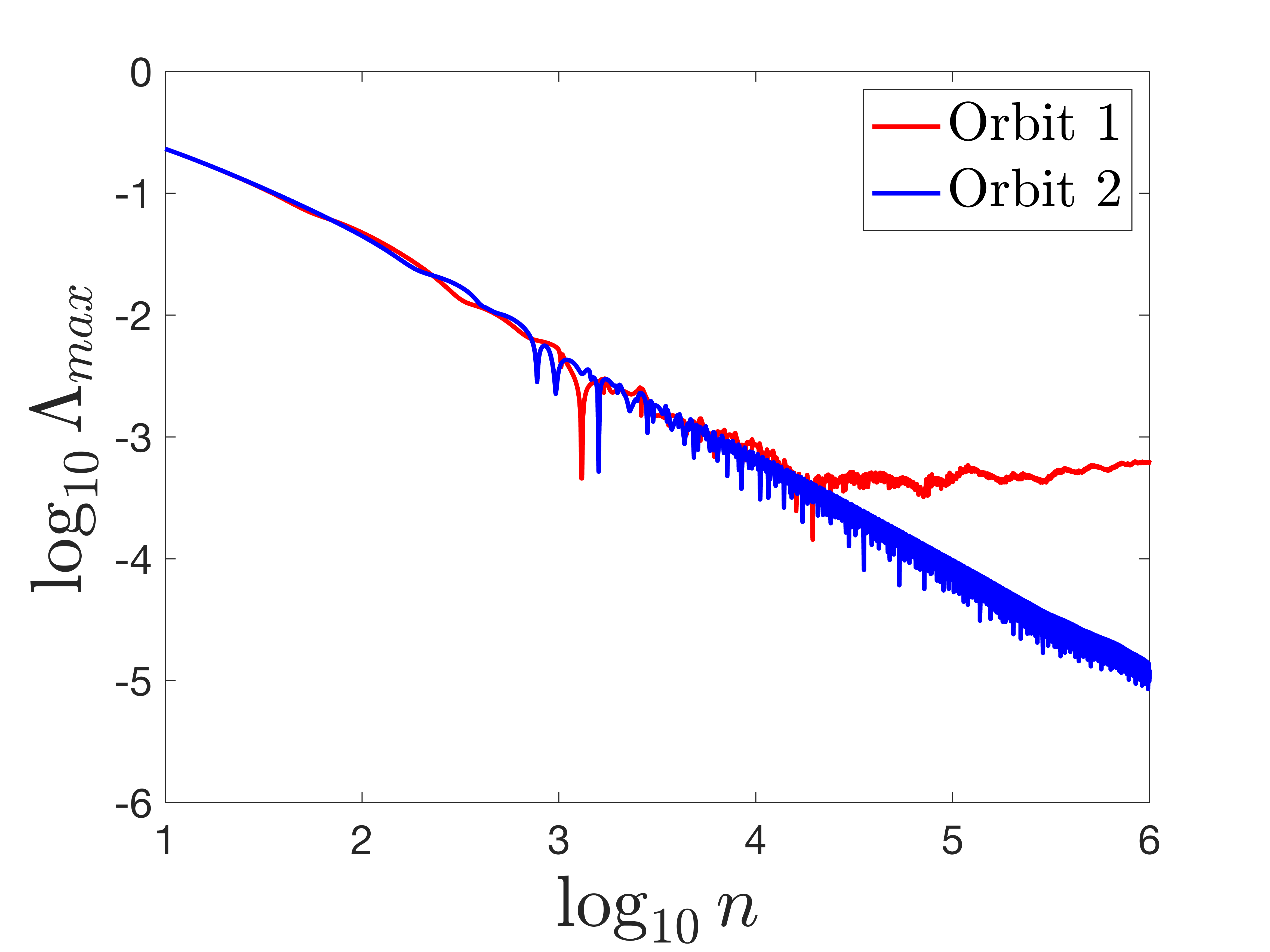
(b) MLE s corresponding to orbit 1 (chaotic) and orbit 2 (regular)

Figure 9: Poincaré sections and corresponding MLE s ($\Lambda_{\text{max}}$) for the orbits with parameters $a=-0.15$, $i=29^{\circ}$, $E=0.965$, $L=5.48$, and $\mathcal{D}=2\times 10^{-4}$.

Before proceeding further, we have checked if the aforementioned scheme of MLE is suitable to distinguish between chaos and order in our system. We have considered two orbits with the same orbital parameters $a=-0.15$, $i=29^{\circ}$, $E=0.965$, $L=5.48$, and $\mathcal{D}=2\times 10^{-4}$. The initial conditions for orbit 1 are $\rho=16$, $p_{\rho}=-0.1$, $z=0$, $p_{z}>0$, and that for orbit 2 are $\rho=23.5$, $p_{\rho}=0.065$, $z=0$, $p_{z}>0$. From the Poincaré plot of sections (Figure 9(a)), we can see that orbit 1 is chaotic in nature, whereas orbit 2 is regular. We evaluated the corresponding MLE s for these two orbits as a function of the number of iterations (Figure 9(b)). We can observe that the scheme can efficiently distinguish between the two orbits for $\left(\log_{10}n\right)\gtrsim 5$. At $n=10^{5}$, the value of MLE for orbit 1 is above the threshold $\Lambda_{\text{max}}=1.5\times 10^{-4}$, and that for orbit 2 is below the threshold, which implies that orbit 1 is chaotic, whereas orbit 2 is regular. Thus, this scheme of MLE works efficiently to distinguish between order and chaos in our system.

By implementing MLE as a quantitative indicator of chaos, we have studied the correlation of chaos with the Kerr parameter $a$ of the COP and the inclination angle $i$ of the orbit. First, let us consider the former. Looking at the overall trends of MLE s, it is evident that the chaoticity of the system has a negative correlation with the rotation parameter $a$ (Figure 10). The inclined orbits are always more chaotic for the maximally counter-rotating COP s, i.e., when the value of $a$ is closer to -1. For lower values of the inclination angle, such as $i=10^{\circ}$ (Figure 10(a)), the degree of chaos decreases gradually with the increasing value of $a$. For higher angles of inclination, the correlation becomes nuanced. It turns out that the degree of chaos weakly depends on the Kerr parameter $a$ for most of its range. However, the chaoticity rapidly increases below a threshold value of the rotation parameter $a=a_{\text{c}}$. For $i=25^{\circ}$ (Figure 10(b)), the threshold value is $a_{\text{c}}\approx-0.85$. When the value of $a$ is more than $a_{\text{c}}=-0.85$, the chaoticity decreases very slowly as $a$ increases. But below $a=a_{\text{c}}$, the MLE increases drastically as $a$ decreases. We observed this qualitatively with the Poincaré Maps in the previous section.

The threshold value of the rotation parameter $a=a_{\text{c}}$ gets affected by the overall chaoticity of the system. Any change in the orbital parameters, which enhances chaoticity in the system, affects it so that the value of $a_{\text{c}}$ increases. For example, for $i=28^{\circ}$ (Figure 10(c)), the threshold value comes out to be $a_{\text{c}}\approx-0.45$. It is more than $a_{\text{c}}\approx-0.85$, which occurs when the inclination was $i=25^{\circ}$ (Figure 10(b)). It is happening because the degree of chaos is enhanced when the inclination angle increases from $i=25^{\circ}$ to $i=28^{\circ}$. It seems like the system tries to sustain its stability as long as possible. However, the enhancement of chaoticity makes the system more nonlinear, causing the system to be stable for a shorter span of the Kerr parameter. That is why the threshold value $a=a_{\text{c}}$ increases and the system retains its stable nature for a shorter range of $a$. When $a<a_{\text{c}}$, the nonlinearity in the system gets triggered, and the MLE shows a sharp upturn as $a$ decreases. We observe a similar phenomenon when we increase energy $E$ and decrease angular momentum $L$ by keeping the inclination angle fixed at $i=25^{\circ}$ (Figure 10(d)). It causes the overall chaoticity to increase, and the threshold value increases from $a_{\text{c}}\approx-0.85$ to $a_{\text{c}}\approx-0.65$.

On the other hand, the dependence of chaoticity on the inclination angle $i$ is opposite to that for the rotation parameter $a$ (Figure 11). The degree of chaos increases in the system as the orbits become more inclined with the rotation axis of the COP while keeping the rest of the orbital parameters fixed. It implies that the thicker accretion disks have more chaotic orbits than the thinner ones. However, the change in the MLE is more rapid at the higher values of the inclination angle. This was also observed earlier while studying the chaotic behaviour of the orbits qualitatively using Poincaré Map plots (Figure 8). There is a sudden increase in the values of MLE s at some threshold value of the inclination angle $i=i_{\text{c}}$ (Figure 11). For $i<i_{\text{c}}$, the chaoticity increases gradually. As the value of $i$ crosses $i_{\text{c}}$, the MLE s start increasing rapidly until it reaches an angle, after which the growth slows down a little, though the positive correlation still holds. This overall trend of MLE s with respect to the inclination angle $i$ is very consistent, and it is true for any given set of orbital parameters.

Now, if we compare Figure 11(a) and Figure 11(b), the threshold value has come down from $i_{\text{c}}\approx 21^{\circ}$ to $i_{\text{c}}\approx 18^{\circ}$ as the dipole coefficient increases from $\mathcal{D}=2\times 10^{-4}$ to $\mathcal{D}=2.2\times 10^{-4}$. These results imply that the value of $i_{\text{c}}$ has an anti-correlation with the degree of chaos in the system. As the chaoticity gets enhanced, the nonlinearity in the system increases, and the value of $i_{\text{c}}$ gets lowered. The explanation of stability, in this case, is similar to what we saw while discussing the dependence of chaoticity on the rotation parameter for the higher values of inclination angles. As before, it seems like the system is trying to sustain its stability as long as possible. But the enhancement in the nonlinearity due to any change in the orbital parameters triggers the system early at a lower value of the inclination angle, and the chaoticity starts increasing rapidly. Thus, the value of $i_{\text{c}}$ gets lowered.

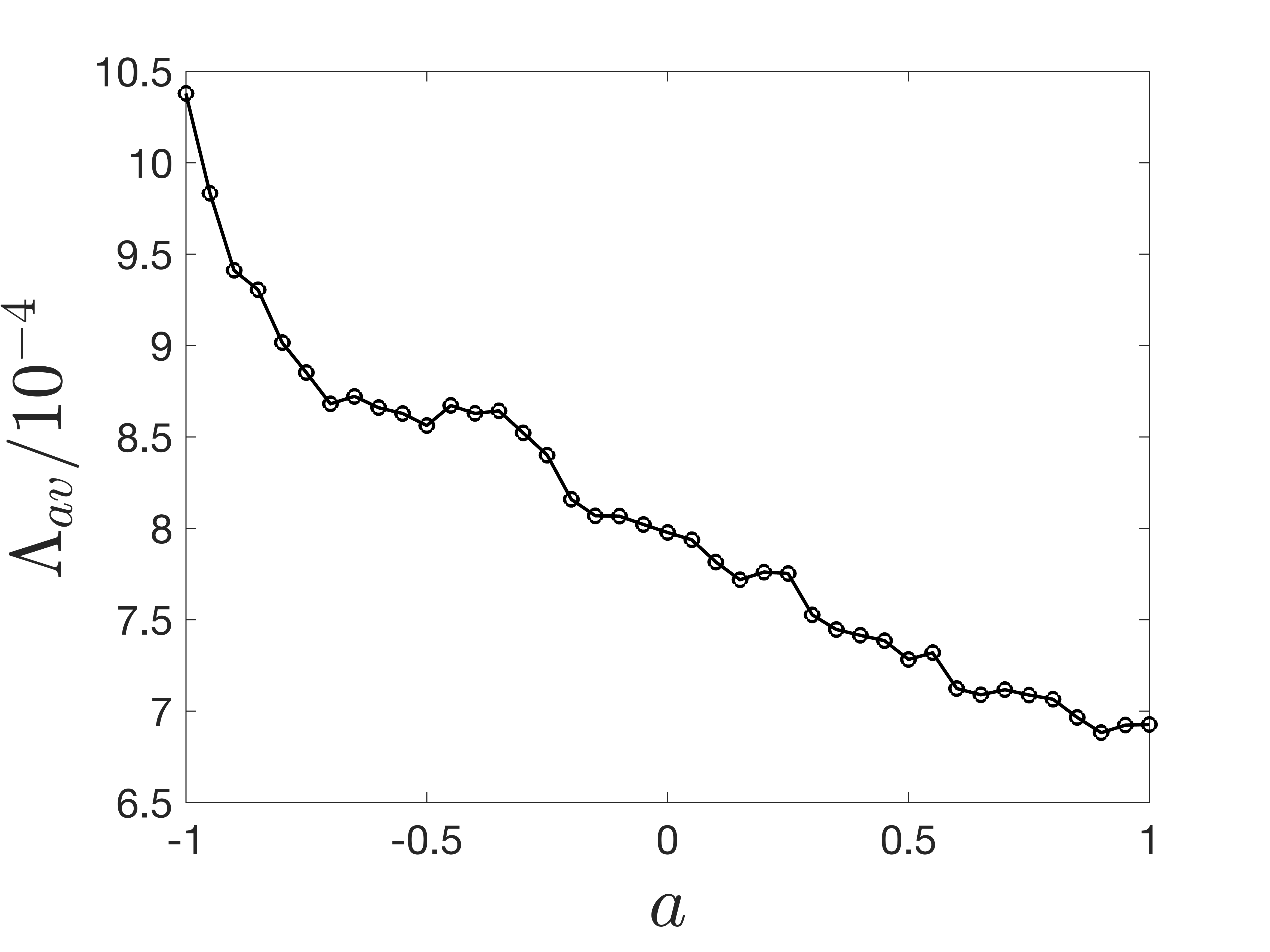
(a) $i=10^{\circ}$, $E=0.976$, $L=4.85$, and $\mathcal{D}=3\times 10^{-4}$

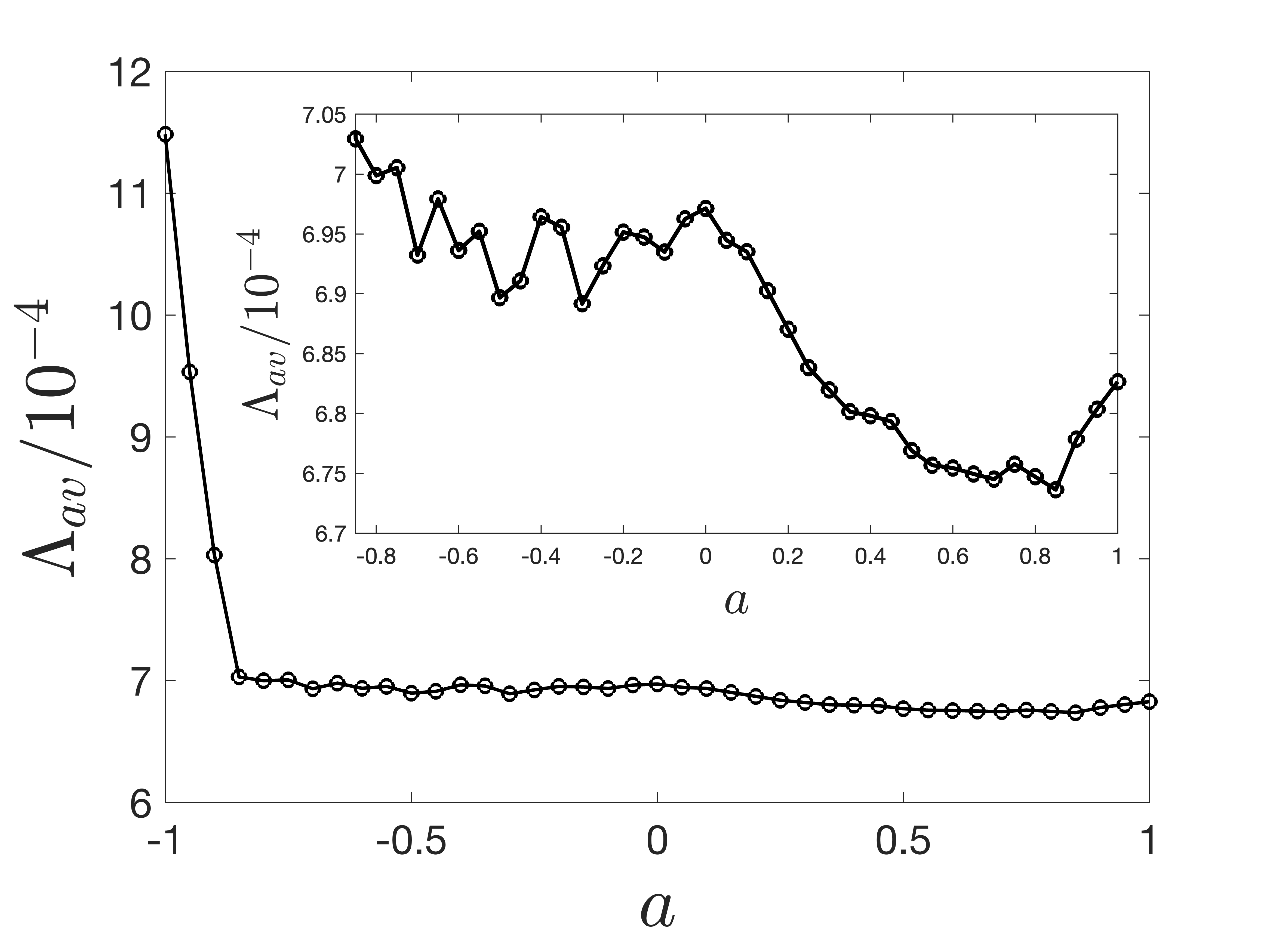
(b) $i=25^{\circ}$, $E=0.9734$, $L=5.82$, and $\mathcal{D}=2\times 10^{-4}$

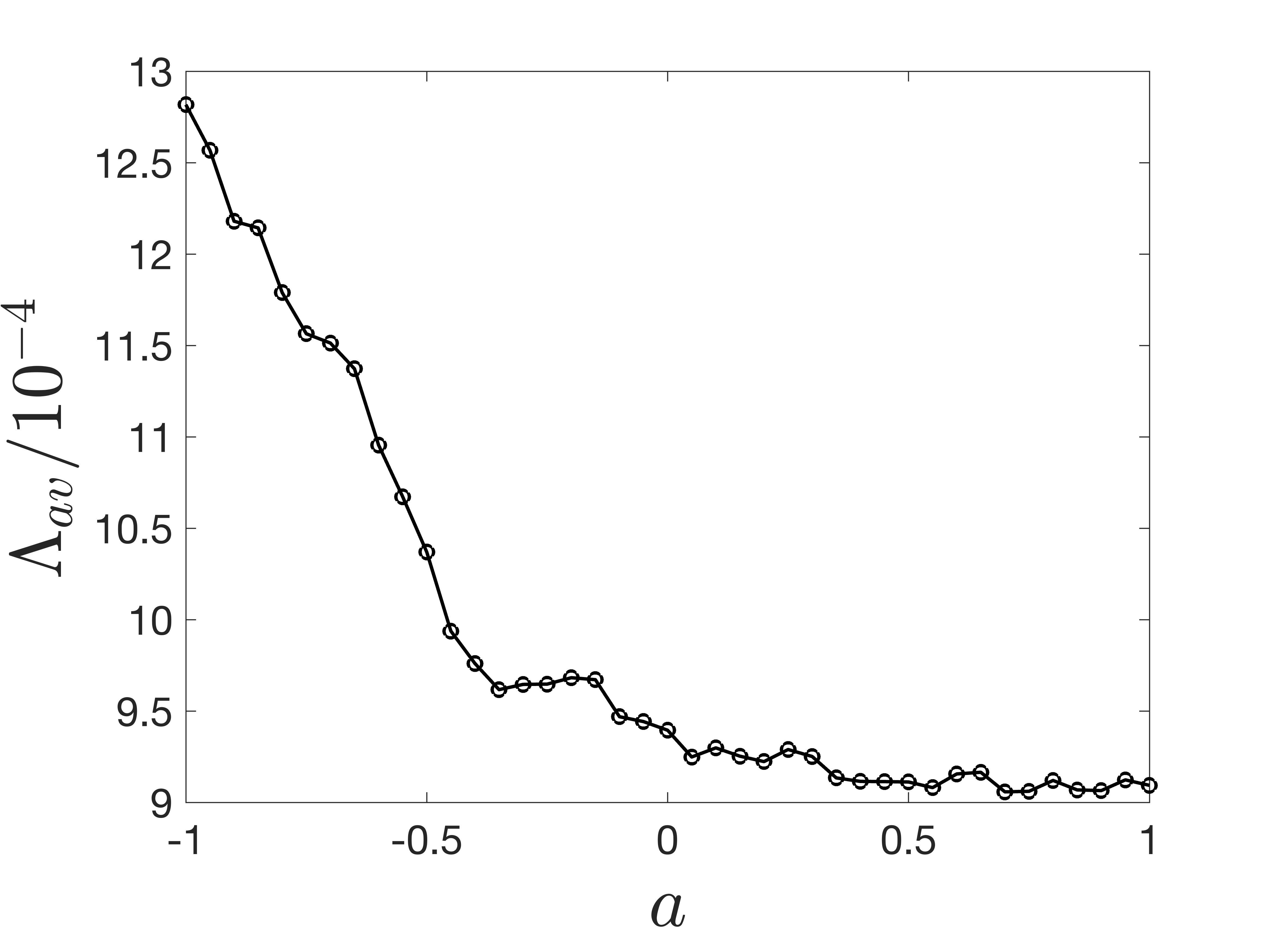
(c) $i=28^{\circ}$, $E=0.9734$, $L=5.82$, and $\mathcal{D}=2\times 10^{-4}$

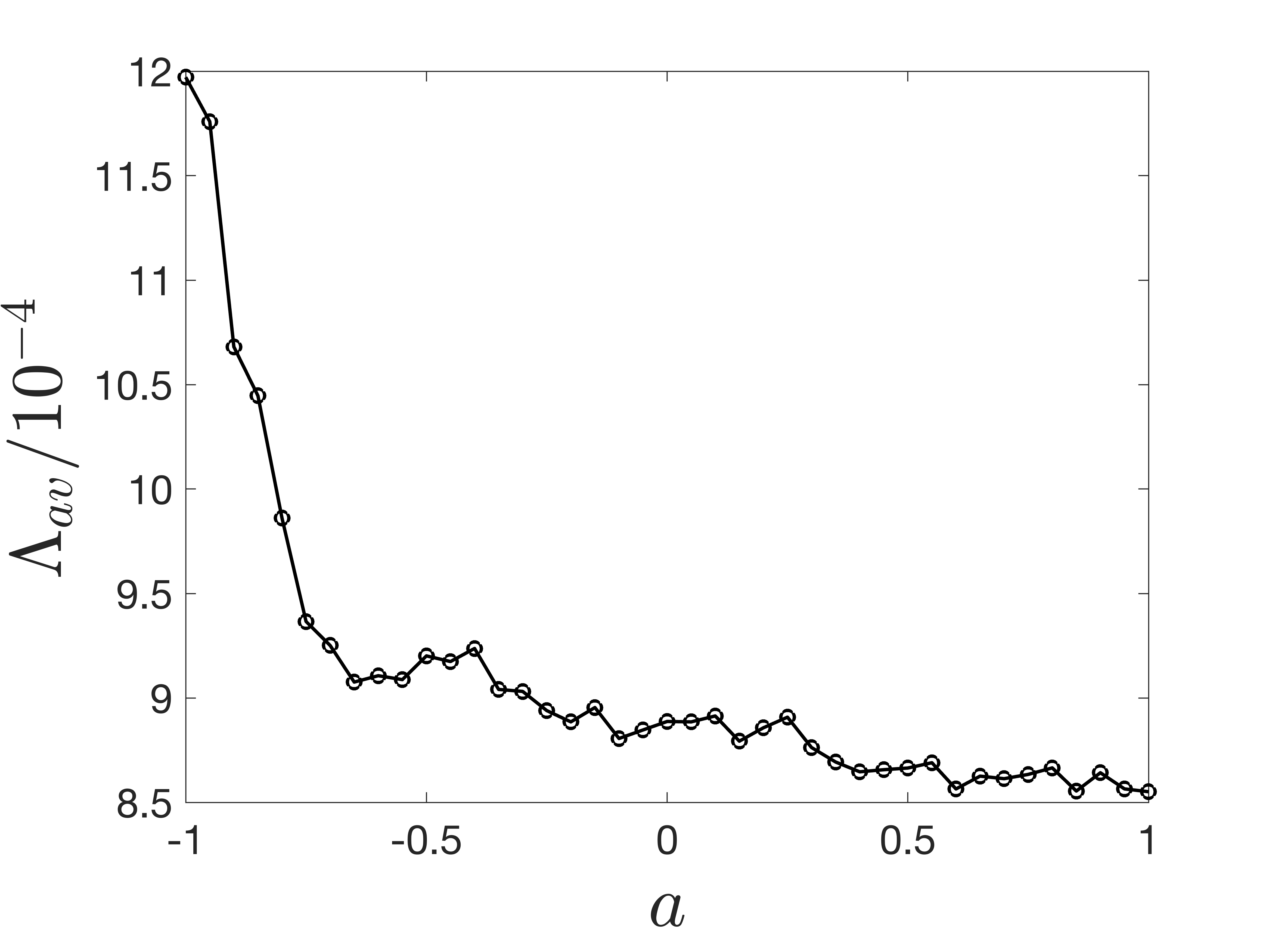
(d) $i=25^{\circ}$, $E=0.9750$, $L=5.72$, and $\mathcal{D}=2\times 10^{-4}$

Figure 10: Maximum Lyapunov Exponent ($\Lambda_{\text{av}}$) as a function of Kerr Parameter $a$.

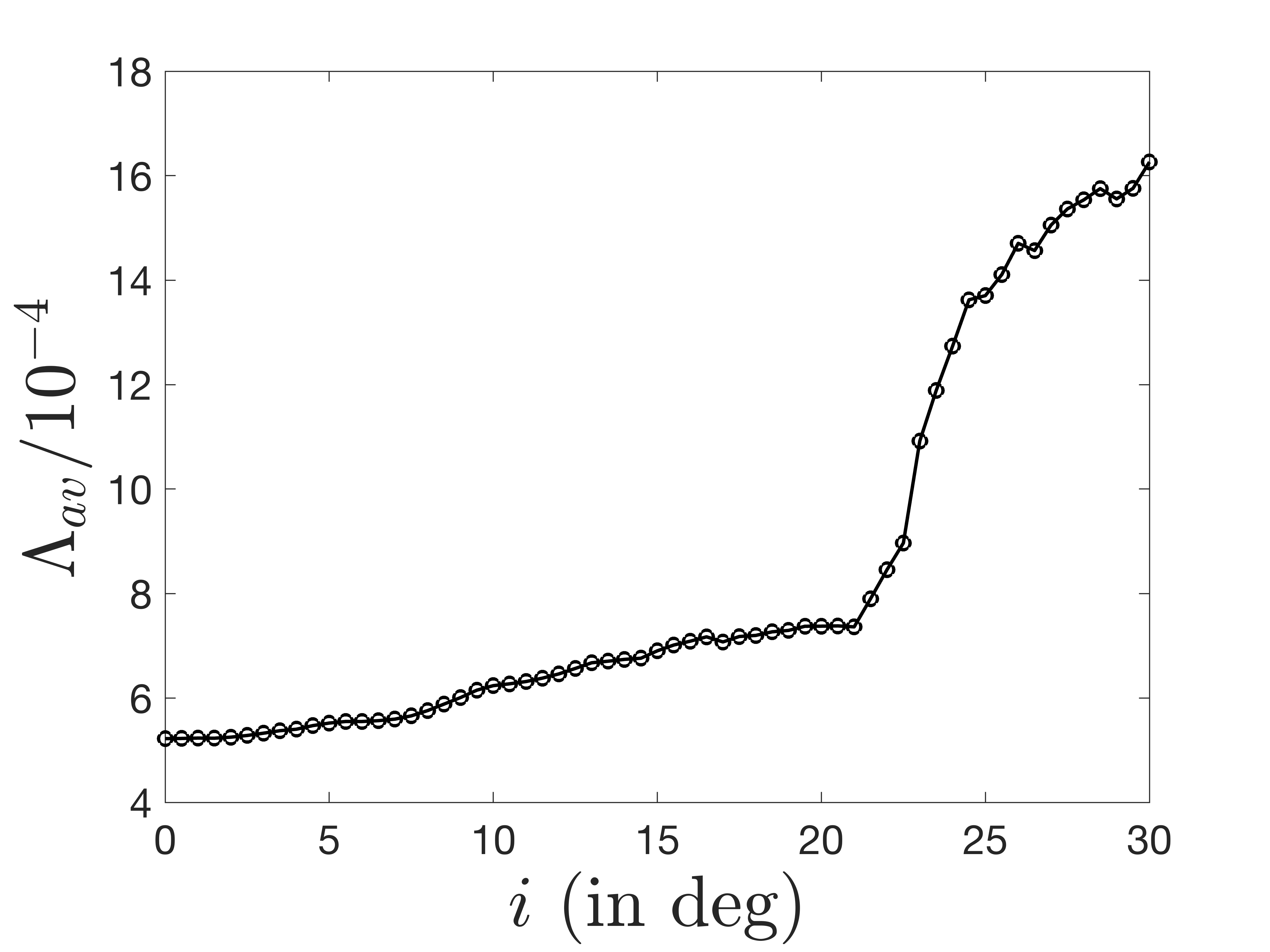
(a) $a=-0.15$, $E=0.976$, $L=4.85$, and $\mathcal{D}=2\times 10^{-4}$

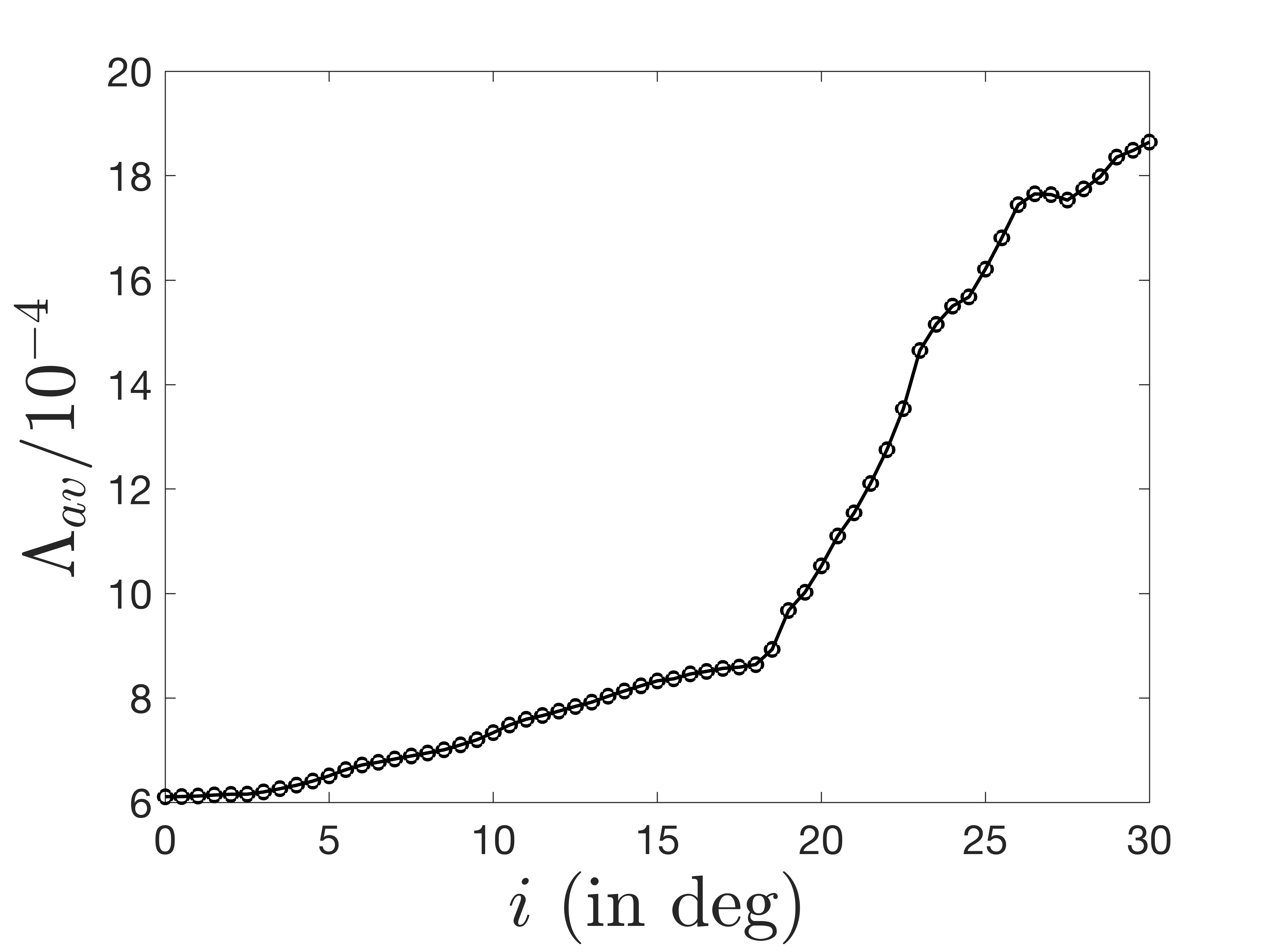
(b) $a=-0.15$, $E=0.976$, $L=4.85$, and $\mathcal{D}=2.2\times 10^{-4}$

Figure 11: Maximum Lyapunov Exponent ($\Lambda_{\text{av}}$) as a function of inclination angle $i$.

5 Conclusions

In the present work, we have studied the chaotic behaviour of the off-equatorial orbits around a pseudo-Newtonian COP using the generalised force presented in Ghosh and Mukhopadhyay [2]. Because of the complex mathematical form of the pseudo-Keplerian force, we have prescribed a numerical method in which a fitting function is used to generate the PNP and implement it in the analysis of orbital dynamics. To incorporate a more realistic scenario, we have introduced an artificial dipolar perturbative term corresponding to an asymmetrically placed hollow halo of matter around the COP. To study the chaotic dynamics of the off-equatorial orbits around the COP, we have implemented the Poincaré Maps and the MLE s as the indicators of chaos. Where Poincaré maps help to visualise chaos qualitatively, MLE s quantify the degree of chaos.

At first, we studied stable circular orbits and observed how their stability gets affected by the Kerr parameter $a$ and the angle of inclination $i$. We have found that the ISCO s are significantly affected by the Kerr parameter compared to the inclination angle. Thereafter, we studied the chaotic dynamics of the generic equatorial orbits governed by the GMf PNP and compared them with those governed by the ABN PNP. We saw that for the orbits around the co-rotating COP s, the GMf PNP induces more chaos into the system. For the orbits around the counter-rotating COP s, the effect is the opposite, i.e., the ABN PNP makes the equatorial orbits more chaotic compared to the GMf PNP.

While studying the correlation of chaos with respect to the rotation parameter $a$, we observed that the chaoticity decreases as the value of $a$ increases. It is maximum for the orbits around the maximally counter-rotating COP s. The degree of chaos for lower values of the inclination angles shows a consistent negative correlation with $a$. Hence, the chaoticity gradually decreases as $a$ increases. However, for higher orbital inclinations, the degree of chaos shows a weak dependence on $a$ at its higher values. Only when $a$ decreases below a threshold value $a_{\text{c}}$, it begins to increase rapidly as $a$ gets lowered. The value of $a_{\text{c}}$ has a positive correlation with the degree of chaos present in the system. If the chaoticity gets enhanced because of the change of any orbital parameters, the value of $a_{\text{c}}$ increases.

We have also established that the chaoticity increases as the orbits become more inclined with the equatorial plane. This has been shown for both Schwarzschild and Kerr-like COP s. The change in the chaotic nature of the orbits is more rapid at higher inclination angles than the lower ones, in which cases the changes are more gradual. The MLE s show a sudden sharp upturn at a particular threshold value of the inclination angle $i=i_{\text{c}}$. For orbits with inclination $i>i_{\text{c}}$, the change in the degree of chaos is more rapid, and for $i<i_{\text{c}}$, the chaoticity changes gradually. Therefore, we can state that for $i>i_{\text{c}}$, even a tiny change in the inclination angle can affect the chaotic behaviour of the orbits significantly. Furthermore, the value of $i_{\text{c}}$ anti-correlates with the nonlinearity in the system. It increases when the overall degree of chaos decreases due to any corresponding change in the orbital parameters.

In future, we would like to perform an in-depth analysis of the dynamics of chaos in the current system using other indicators of chaos, namely the Fast Lyapunov Index or FLI [71, 58], Small Alignment Index or SALI [72, 73], and General Alignment Index or GALI [74], which are more sensitive to chaos than MLE, making them more efficient to distinguish between order and chaos. We would also like to implement the PNP to study the off-axis motion of a test particle in a restricted three-body system, where the other two bodies are pseudo-Newtonian compact object binaries.

Data Availability

No data was used for the research described in the article.

References

- Artemova et al. [1996] I. V. Artemova, G. Björnsson, I. D. Novikov, Modified newtonian potentials for the description of relativistic effects in accretion disks around black holes, ApJ 461 (1996) 565.
- Ghosh and Mukhopadhyay [2007] S. Ghosh, B. Mukhopadhyay, Generalized pseudo-newtonian potential for studying accretion disk dynamics in off-equatorial planes around rotating black holes: Description of a vector potential, ApJ 667 (2007) 367.
- Paczynsky and Wiita [1980] B. Paczynsky, P. J. Wiita, Thick accretion disks and supercritical luminosities, A&A 88 (1980) 23–31.
- Nag et al. [2017] S. Nag, S. Sinha, D. B. Ananda, T. K. Das, Influence of the black hole spin on the chaotic particle dynamics within a dipolar halo, Ap&SS 362 (2017) 81.
- Polcar et al. [2019] L. Polcar, P. Suková, O. Semerák, Free motion around black holes with disks or rings: Between integrability and chaos–v, ApJ 877 (2019) 16.
- Dubeibe et al. [2021] F. L. Dubeibe, T. Saeed, E. E. Zotos, Effect of multipole moments in the weak field limit of a black hole plus halo potential, ApJ 908 (2021) 74.
- Dubeibe et al. [2017] F. Dubeibe, F. Lora-Clavijo, G. A. González, Pseudo-newtonian planar circular restricted 3-body problem, Phys. Lett. A 381 (2017) 563–567.
- De et al. [2021] S. De, S. Roychowdhury, R. Banerjee, Beyond-newtonian dynamics of a planar circular restricted three-body problem with kerr-like primaries, MNRAS 501 (2021) 713–729.
- Alrebdi et al. [2022] H. Alrebdi, K. E. Papadakis, F. L. Dubeibe, E. E. Zotos, Equilibrium points and networks of periodic orbits in the pseudo-newtonian planar circular restricted three-body problem, Astron. J. 163 (2022) 75.
- Kormendy and Richstone [1995] J. Kormendy, D. Richstone, Inward bound—the search for supermassive black holes in galactic nuclei, Annual review of A&A 33 (1995) 581–624.
- Beckmann and Shrader [2012] V. Beckmann, C. Shrader, Active galactic nuclei, John Wiley & Sons, 2012.
- Panagia et al. [1996] N. Panagia, S. Scuderi, R. Gilmozzi, P. Challis, P. Garnavich, R. Kirshner, On the nature of the outer rings around sn 1987a, ApJ 459 (1996) L17.
- Meyer [1997] F. Meyer, Formation of the outer rings of supernova 1987a, MNRAS 285 (1997) L11–L14.
- Vieira and Letelier [1999] W. M. Vieira, P. S. Letelier, Relativistic and newtonian core-shell models: analytical and numerical results, ApJ 513 (1999) 383.
- Sackett and Sparke [1990] P. D. Sackett, L. S. Sparke, The dark halo of the polar-ring galaxy ngc 4650a, ApJ 361 (1990) 408–418.
- Arnaboldi et al. [1993] M. Arnaboldi, M. Capaccioli, E. Cappellaro, E. V. Held, L. Sparke, Studies of narrow polar rings around e galaxies. i-observations and model of am 2020-504, A&A 267 (1993) 21–30.
- Reshetnikov and Sotnikova [1997] V. Reshetnikov, N. Sotnikova, Global structure and formation of polar-ring galaxies, arXiv preprint astro-ph/9704047 (1997).
- Malin and Carter [1983] D. Malin, D. Carter, A catalog of elliptical galaxies with shells, ApJ 274 (1983) 534–540.
- Quinn [1984] P. J. Quinn, On the formation and dynamics of shells around elliptical galaxies, ApJ 279 (1984) 596–609.
- Dupraz and Combes [1987] C. Dupraz, F. Combes, Dynamical friction and shells around elliptical galaxies, A&A 185 (1987) L1–L4.
- Vieira and Letelier [1996] W. M. Vieira, P. S. Letelier, Chaos around a hénon-heiles-inspired exact perturbation of a black hole, Phys. Rev. Lett. 76 (1996) 1409.
- Letelier and Vieira [1997] P. Letelier, W. Vieira, Chaos and rotating black holes with halos, Phys. Rev. D 56 (1997) 8095.
- Guéron and Letelier [2002] E. Guéron, P. S. Letelier, Geodesic chaos around quadrupolar deformed centers of attraction, Phys. Rev. E 66 (2002) 046611.
- Vogt and Letelier [2003] D. Vogt, P. S. Letelier, Exact general relativistic perfect fluid disks with halos, Phys. Rev. D 68 (2003) 084010.
- Semerák and Suková [2010] O. Semerák, P. Suková, Free motion around black holes with discs or rings: between integrability and chaos–i, MNRAS 404 (2010) 545–574.
- Semerák and Suková [2012] O. Semerák, P. Suková, Free motion around black holes with discs or rings: between integrability and chaos–ii, MNRAS 425 (2012) 2455–2476.
- Suková and Semerák [2013] P. Suková, O. Semerák, Free motion around black holes with discs or rings: between integrability and chaos–iii, MNRAS 436 (2013) 978–996.
- Janiuk and Czerny [2011] A. Janiuk, B. Czerny, On different types of instabilities in black hole accretion discs: implications for x-ray binaries and active galactic nuclei, MNRAS 414 (2011) 2186–2194.
- Witzany et al. [2015] V. Witzany, O. Semerák, P. Suková, Free motion around black holes with discs or rings: between integrability and chaos–iv, MNRAS 451 (2015) 1770–1794.
- Kopáček and Karas [2014] O. Kopáček, V. Karas, Inducing chaos by breaking axial symmetry in a black hole magnetosphere, ApJ 787 (2014) 117.
- Kopáček and Karas [2015] O. Kopáček, V. Karas, Regular and chaotic motion in general relativity: The case of an inclined black hole magnetosphere, Journal of Physics: Conference Series 600 (2015) 012070.
- Takahashi and Koyama [2009] M. Takahashi, H. Koyama, Chaotic motion of charged particles in an electromagnetic field surrounding a rotating black hole, ApJ 693 (2009) 472.
- De Falco and Borrelli [2021a] V. De Falco, W. Borrelli, Detection of chaos in the general relativistic poynting-robertson effect: Kerr equatorial plane, Phys. Rev. D 103 (2021a) 064014.
- De Falco and Borrelli [2021b] V. De Falco, W. Borrelli, Timescales of the chaos onset in the general relativistic poynting-robertson effect, Phys. Rev. D 103 (2021b) 124012.
- Miller et al. [2009] J. M. Miller, C. S. Reynolds, A. C. Fabian, G. Miniutti, L. C. Gallo, Stellar-mass black hole spin constraints from disk reflection and continuum modeling, ApJ 697 (2009) 900.
- Ziolkowski [2010] J. Ziolkowski, Population of galactic black holes., Memorie della Società Astronomica Italiana 81 (2010) 294.
- Daly [2011] R. A. Daly, Estimates of black hole spin properties of 55 sources, MNRAS 414 (2011) 1253–1262.
- Reynolds et al. [2012] C. S. Reynolds, L. W. Brenneman, A. M. Lohfink, M. L. Trippe, J. M. Miller, R. C. Reis, M. A. Nowak, A. C. Fabian, Probing relativistic astrophysics around smbhs: The suzaku agn spin survey, AIP Conference Proceedings 1427 (2012) 157–164.
- Dotti et al. [2012] M. Dotti, M. Colpi, S. Pallini, A. Perego, M. Volonteri, On the orientation and magnitude of the black hole spin in galactic nuclei, ApJ 762 (2012) 68.
- Tchekhovskoy and McKinney [2012] A. Tchekhovskoy, J. C. McKinney, Prograde and retrograde black holes: whose jet is more powerful?, MNRAS: Letters 423 (2012) L55–L59.
- Garofalo [2013] D. Garofalo, Retrograde versus prograde models of accreting black holes, Advances in Astronomy 2013 (2013) 213105.
- Healy et al. [2014] J. Healy, C. O. Lousto, Y. Zlochower, Remnant mass, spin, and recoil from spin aligned black-hole binaries, Phys. Rev. D 90 (2014) 104004.
- Sesana et al. [2014] A. Sesana, E. Barausse, M. Dotti, E. M. Rossi, Linking the spin evolution of massive black holes to galaxy kinematics, ApJ 794 (2014) 104.
- Nowak and Wagoner [1991] M. A. Nowak, R. V. Wagoner, Diskoseismology: Probing accretion disks. i-trapped adiabatic oscillations, ApJ 378 (1991) 656–664.
- Chakrabarti and Khanna [1992] S. K. Chakrabarti, R. Khanna, A newtonian description of the geometry around a rotating black hole, MNRAS 256 (1992) 300–306.
- Semerák and Karas [1999] O. Semerák, V. Karas, Pseudo-newtonian models of a rotating black hole field, A&A 343 (1999) 325–332.
- Mukhopadhyay [2002] B. Mukhopadhyay, Description of pseudo-newtonian potential for the relativistic accretion disks around kerr black holes, ApJ 581 (2002) 427.
- Mukhopadhyay and Misra [2003] B. Mukhopadhyay, R. Misra, Pseudo-newtonian potentials to describe the temporal effects on relativistic accretion disks around rotating black holes and neutron stars, ApJ 582 (2003) 347.
- Ghosh [2004] S. Ghosh, Rotating central objects with hard surfaces: A pseudo-newtonian potential for relativistic accretion disks, A&A 418 (2004) 795–799.
- Chakrabarti and Mondal [2006] S. K. Chakrabarti, S. Mondal, Studies of accretion flows around rotating black holes–i. particle dynamics in a pseudo-kerr potential, MNRAS 369 (2006) 976–984.
- Kovář et al. [2008] J. Kovář, Z. Stuchlík, V. Karas, Off-equatorial orbits in strong gravitational fields near compact objects, Class. Quant. Grav. 25 (2008) 095011.
- Kovář et al. [2010] J. Kovář, O. Kopáček, V. Karas, Z. Stuchlík, Off-equatorial orbits in strong gravitational fields near compact objects—ii: halo motion around magnetic compact stars and magnetized black holes, Class. Quant. Grav. 27 (2010) 135006.
- Barausse et al. [2007] E. Barausse, S. A. Hughes, L. Rezzolla, Circular and noncircular nearly horizon-skimming orbits in kerr spacetimes, Phys. Rev. D 76 (2007) 044007.
- Gueron and Letelier [2001] E. Gueron, P. S. Letelier, Chaos in pseudo-newtonian black holes with halos, A&A 368 (2001) 716–720.
- Guéron and Letelier [2001] E. Guéron, P. S. Letelier, Chaotic motion around prolate deformed bodies, Phys. Rev. E 63 (2001) 035201.
- Chen and Wang [2003] J. Chen, Y. Wang, Chaotic dynamics of a test particle around a gravitational field with a dipole, Class. Quant. Grav. 20 (2003) 3897.
- Letelier et al. [2011] P. S. Letelier, J. Ramos-Caro, F. López-Suspes, Chaotic motion in axially symmetric potentials with oblate quadrupole deformation, Phys. Lett. A 375 (2011) 3655–3658.
- Wang and Wu [2012] Y. Wang, X. Wu, Dynamics of particles around a pseudo-newtonian kerr black hole with halos, Chinese Physics B 21 (2012) 050504.
- Ghosh et al. [2014] S. Ghosh, T. Sarkar, A. Bhadra, Newtonian analogue of corresponding space–time dynamics of rotating black holes: implication for black hole accretion, MNRAS 445 (2014) 4460–4476.
- Bhattacharya et al. [2010] D. Bhattacharya, S. Ghosh, B. Mukhopadhyay, Disk-outflow coupling: Energetics around spinning black holes, ApJ 713 (2010) 105.
- Steklain and Letelier [2009] A. Steklain, P. Letelier, Stability of orbits around a spinning body in a pseudo-newtonian hill problem, Phys. Lett. A 373 (2009) 188–194.
- Lense and Thirring [1918] J. Lense, H. Thirring, On the influence of the proper rotation of a central body on the motion of the planets and the moon, according to einstein’s theory of gravitation, Phys. Z. 19 (1918) 156.
- Binney and Tremaine [2008] J. Binney, S. Tremaine, Galactic dynamics, 2nd ed., Princeton University Press, USA, 2008.
- Wang and Wu [2011] Y. Wang, X. Wu, Gravitational waves from a pseudo-newtonian kerr field with halos, Commun. Theor. Phys. 56 (2011) 1045.
- Shapiro and Teukolsky [1983] S. L. Shapiro, S. A. Teukolsky, Black holes, white dwarfs, and neutron stars: The physics of compact objects, New York: Wiley, 1983.
- Berry [1978] M. V. Berry, Topics in nonlinear dynamics; jorna, s. (ed.), Am. Inst. Phys. Conf. Proc. 46 (1978) 16.
- Goldstein et al. [2001] H. Goldstein, C. Pool, J. Safko, Classical Mechanics, 3rd ed., Addison Wesley, USA, 2001.
- Strogatz [2007] S. H. Strogatz, Nonlinear dynamics and chaos: with applications to physics, biology, chemistry, and engineering, Sarat Book House, Kolkata, 2007.
- Skokos and Gerlach [2010] C. Skokos, E. Gerlach, Numerical integration of variational equations, Phys. Rev. E 82 (2010) 036704.
- Tancredi et al. [2001] G. Tancredi, A. Sánchez, F. Roig, A comparison between methods to compute lyapunov exponents, AJ 121 (2001) 1171.
- Froeschlé et al. [1997] C. Froeschlé, E. Lega, R. Gonczi, Fast lyapunov indicators. application to asteroidal motion, Celest. Mech. Dyn. Astr. 67 (1997) 41–62.
- Skokos [2001] C. Skokos, Alignment indices: a new, simple method for determining the ordered or chaotic nature of orbits, Journal of Physics A: Mathematical and General 34 (2001) 10029.
- Skokos et al. [2004] C. Skokos, C. Antonopoulos, T. Bountis, M. Vrahatis, Detecting order and chaos in hamiltonian systems by the sali method, Journal of Physics A: Mathematical and General 37 (2004) 6269.
- Skokos et al. [2007] C. Skokos, T. Bountis, C. Antonopoulos, Geometrical properties of local dynamics in hamiltonian systems: The generalized alignment index (gali) method, Physica D: Nonlinear Phenomena 231 (2007) 30–54.