Geometry-Aware Attenuation Field Learning for Sparse-View CBCT Reconstruction

Abstract

Cone Beam Computed Tomography (CBCT) is the most widely used imaging method in dentistry. As hundreds of X-ray projections are needed to reconstruct a high-quality CBCT image (i.e., the attenuation field) in traditional algorithms, sparse-view CBCT reconstruction has become a main focus to reduce radiation dose. Several attempts have been made to solve it while still suffering from insufficient data or poor generalization ability for novel patients. This paper proposes a novel attenuation field encoder-decoder framework by first encoding the volumetric feature from multi-view X-ray projections, then decoding it into the desired attenuation field. The key insight is when building the volumetric feature, we comply with the multi-view CBCT reconstruction nature and emphasize the view consistency property by geometry-aware spatial feature querying and adaptive feature fusing. Moreover, the prior knowledge information learned from data population guarantees our generalization ability when dealing with sparse view input. Comprehensive evaluations have demonstrated the superiority in terms of reconstruction quality, and the downstream application further validates the feasibility of our method in real-world clinics.

1 Introduction

Cone Beam Computed Tomography (CBCT), a variant of CT scanning, is the most widely used imaging technique in dentistry since it provides 3D structure information with higher spatial resolution using shorter scanning time. The standard imaging scheme of CBCT is illustrated in Fig. 1. During CBCT scanning, an X-ray source uniformly moves along an arc-shaped orbit and emits a cone-shaped beam towards the interested organ (e.g., oral cavity) for each angular step. And, the detector on the opposite side of the patient captures a 2D perspective projection. CBCT reconstruction aims to recover a 3D attenuation field (i.e., CBCT image) from such 2D projections in an inverse manner. This is primarily achieved based on the Filtered Back Projection (FBP) algorithm [3], which, however, typically requires hundreds of projections and results in a high radiation exposure. Thus, sparse-view (e.g., 5, or 10 views) CBCT reconstruction by reducing the number of projection views has received widespread attention in the research field.

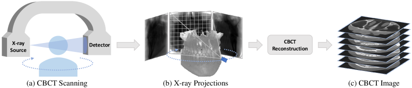
Figure 1: CBCT Imaging: (a) CBCT scanning would produce a series of (b) X-ray projections, which will be used to solve (c) a 3D CBCT image through CBCT reconstruction.

Sparse-view CBCT reconstruction is a challenging task due to data insufficiency. To address this problem, many traditional methods exploited the consistency between the acquired projections and the reconstructed image. For example, SART [1] proposes an iterative strategy that minimizes the difference between 2D projections and their estimates while updating the 3D attenuation field. It is effective under noisy and insufficient data, but still compromises image quality while more computationally demanding. With the advance of deep learning, some learning-based methods are designed to learn the common knowledge from data population [5, 11, 14], benefiting from the generalization ability of convolution networks. These frameworks are based on an encoder-decoder structure, where the 2D encoder learns the feature representations of given projections, which are then combined and transferred into 3D by simply reshaping, following a 3D decoder to generate the volumetric image. While these methods can provide decent reconstructed images, they often lack important fine details and tend to be over-smooth. This is mainly due to the brute-force concatenation of multiple fix-posed projections that completely ignores their spatial view and geometric relationships. Recently, another line of methods, neural rendering [8], appears to be an emerging technique for novel view synthesis, which also targets an inverse rendering problem similar to CBCT reconstruction. However, CBCT reconstruction aims for the entire volumetric attenuation field (See Fig. 1), while neural rendering in computer vision society merely approximates the surface of interested objects. NAF [16] first adapts this technique for sparse-view CBCT reconstruction, and leverages multi-resolution hash encoding [9] to achieve promising performance with only 50 projections. It benefits from 3D geometry awareness and multi-view consistency of neural rendering, preserving fine details despite the input being less sufficient. Unfortunately, without generalization ability, NAF relies on time-consuming per-scene optimization, typically taking tens of minutes for one subject, and does not tackle the sparse-view problem thoroughly, making it struggle to produce reliable quality when giving very limited projections (e.g., 5 or 10 views).

In this paper, we propose a novel encoder-decoder framework of geometry-aware attenuation field learning for sparse-view CBCT reconstruction, enjoying both the generalization ability of learning-based methods and the geometry-aware view consistency of multi-view reconstruction (e.g., neural rendering). Specifically, we first adopt CNN feature extraction to encode the X-ray projections. And then, when building volumetric features, we emphasize view consistency by geometry-aware feature querying from different projections. Furthermore, to consider the importance of different views, we utilize adaptive feature fusing to aggregate multi-view features into point-wise attenuation feature vectors. In this way, a 3D attenuation feature field is formed, and finally, decoded through attenuation field decoding to the desired resolution of the CBCT image. Our framework is flexible for both input poses and the number of views. And thanks to the prior knowledge learned from the data population, our method can naturally generalize to other patients without further training and efficiently produce high-quality reconstruction given very limited input views (e.g., 5 or 10 views). Experiments have demonstrated the superior reconstruction quality of our method, which is further verified by potential downstream applications, e.g., tooth segmentation.

2 Method

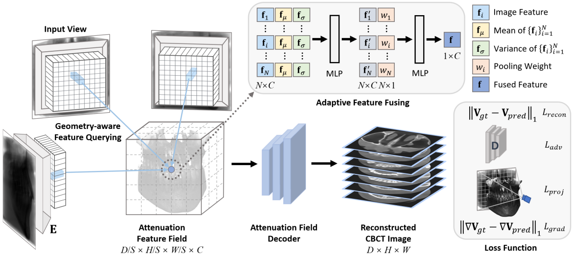
Figure 2: Illustration of our proposed method to achieve 3D CBCT image reconstruction via 2D X-ray projections.

2.1 Geometry-Aware Attenuation Field Learning

2.1.1 CNN Feature Extraction

According to Fig. 1, the 3D attenuation field is solved with 2D X-ray projections in an inverse rendering manner. An intuitive idea is to extract the feature representations of these projections, and use them to learn the mapping to the attenuation field. Specifically, given $N$ projections $\{\mathbf{I}_{i}\}^{N}_{i=1}$, we exploit a 2D CNN encoder $\mathbf{E}$ (ResNet34 [4] in our work) to extract 2D feature representations, denoted as $\{\mathbf{F}_{i}=\mathbf{E}(\mathbf{I}_{i})\}^{N}_{i=1}$.

2.1.2 Geometry-Aware Feature Querying

The key insight of our framework is the generalizable attenuation field learning with geometry awareness. As illustrated in Fig. 2, we aim to fetch the attenuation feature field in the world coordinate, by querying the 2D feature representations in the pixel coordinate. In this step, we sample 3D query points on a sparse voxel grid, then project each query point onto all feature representations $\{\mathbf{F}_{i}\}_{i=1}^{N}$ respectively, by utilizing their camera pose information to make a transformation between the world and pixel coordinates. For $\mathbf{F}_{i}$, we denote its extrinsic camera matrix as $\mathbf{M}^{(i)}=[\mathbf{R}^{(i)}\ \mathbf{t}^{(i)}]$ and intrinsic camera matrix as $\mathbf{K}^{(i)}$, where $\mathbf{R}^{(i)}$ denotes rotation and $\mathbf{t}^{(i)}$ denotes translation. Then, for each 3D query point $\mathbf{x}$ in the world coordinate, we transform it into the corresponding pixel coordinate $\mathbf{x}^{(i)}_{uv}$ of $\mathbf{F}_{i}$ as follows:

$$\mathbf{x}^{(i)}_{uv}=\mathbf{K}^{(i)}\mathbf{M}^{(i)}\mathbf{x},$$ (1)

we can then get the feature vector of $\mathbf{x}$ from $\mathbf{F}_{i}$ by bilinear interpolation:

$$\mathbf{f}_{i}=\mathbf{F}_{i}(\mathbf{x}^{(i)}_{uv}),i=1,2,...,N$$ (2)

where $\mathbf{f}_{i}\in\mathbb{R}^{C}$. In this way, we can obtain spatial consistent feature vectors $\{\mathbf{f}_{i}\}_{i=1}^{N}$ of a query point $\mathbf{x}$ from all 2D feature representations $\{\mathbf{F}_{i}\}_{i=1}^{N}$.

2.1.3 Adaptive Feature Fusing

After acquiring multi-view feature vectors $\{\mathbf{f}_{i}\}_{i=1}^{N}$ of a query point $\mathbf{x}$ by feature querying, we aim to fuse them into an attenuation feature vector $\mathbf{f}$. However, because of the diverse spatial positioning of query points, a specific query point $\mathbf{x}$ may receive different attenuation information from different views. Therefore, inspired by [12], we design an adaptive feature fusing strategy to aggregate these feature vectors. Specifically, for $\{\mathbf{f}_{i}\}_{i=1}^{N}$ of the query point $\mathbf{x}$, we compute an element-wise mean vector $\mathbf{f}_{\mu}\in\mathbb{R}^{C}$ and variance vector $\mathbf{f}_{\sigma}\in\mathbb{R}^{C}$ to capture global information. We consider each $\mathbf{f}_{i}$ as local information from the $i$-th view, and integrate it with both $\mathbf{f}_{\mu}$ and $\mathbf{f}_{\sigma}$ as global information by concatenation. The concatenated feature is fed into the first MLP to aggregate both local and global information, producing an aggregated global-aware feature vector $\mathbf{f}^{{}^{\prime}}_{i}\in\mathbb{R}^{C}$ and a normalized pooling weight $w_{i}\in[0,1]$ for each view, which are weighted summed together and sent into the second MLP to obtain the final fused feature $\mathbf{f}\in\mathbb{R}^{C}$. Notice that the pooling weight $w_{i}$ can be considered as the contributing factor of the $i$-th view.

2.1.4 Attenuation Field Decoding

After obtaining the attenuation feature vector $\mathbf{f}$ of each query point, we can then build the attenuation feature field by combining all query points together. Limited by the memory size of hardware devices, we build a low-resolution attenuation feature voxel grid with a downsampled size of $D/S\times\!H/S\times\!W/S\times\!C$, which greatly accelerates computation. This attenuation feature field can be considered as the feature representation of the target CBCT image. Thus, we feed it into the attenuation field decoder to obtain the target volumetric attenuation field (i.e., a CBCT image) in the desired resolution $D\times\!H\times\!W$.

2.2 Model Optimization

We mainly use the ground truth volumetric attenuation values to supervise the training of our framework. We first define the reconstruction loss $L_{recon}$ as the L1 loss between ground truth $\mathbf{V}_{gt}$ and the prediction $\mathbf{V}_{pred}$ to enforce voxel-wise similarity. We also apply patch discrimination [17] to improve reconstruction quality, with a least-squares adversarial loss $L_{adv}$ [7]. To recover fine-grained details, we further introduce gradient loss $L_{grad}$ as L1 loss between the first order differential of ground truth $\nabla\mathbf{V}_{gt}$ and the one of prediction $\nabla\mathbf{V}_{pred}$. Particularly, similar to neural rendering based methods [8, 16], we also introduce a self-supervised 2D projection loss $L_{proj}$, by minimizing the L1 loss between a random batch $\mathbf{B}$ of DRR-rendered pixels and their ground truth during the training stage. Therefore, our final objective function is defined as:

$$L=L_{recon}+\lambda_{adv}L_{adv}+\lambda_{grad}L_{grad}+\lambda_{proj}L_{proj},$$ (3)

where $\lambda_{adv}$, $\lambda_{grad}$, and $\lambda_{proj}$ are used to control importance of different terms.

3 Experiments

3.1 Experimental Settings

3.1.1 Dataset

In clinical practice, paired 2D X-ray projections and 3D CBCT images are very scarce. Thus, we address this challenge by generating multiple X-ray projections from the collected CBCT image using the Digitally Reconstructed Radiography (DRR) technique, i.e., we conduct the process as shown in Fig. 1 and utilize Beer’s Law to simulate the attenuation of X-ray during scanning. In total, our dataset consists of 130 dental CBCT images of different patients with a resolution of $256\times 256\times 256$. We split it into 100 images for training, 10 for validating, and 20 for testing. For each CBCT image, the corresponding X-ray projections are produced as described above. In our experiments, we generate $N$ X-ray projections for every $360/N$ degree around the center of the CBCT image, where each X-ray projection has a resolution of $256\times 256$. We select $N=5,~{}10,~{}\text{and}~{}20$ throughout this paper.

3.1.2 Implementation Details

In experiments, we empirically set $\lambda_{adv}=0.001$, $\lambda_{proj}=0.01$, $\lambda_{grad}=1$, the downsampling rate $S=4$, the channel size $C=256$, and the DRR ray batch size $|\mathbf{B}|=1024$. We use Adam optimizer with a learning rate of 1$\times 10^{-4}$, which decays by 0.5 for every 50 epochs, and the training process ends after 150 epochs. The decoder and discriminator are 3D implementation of SRGAN [6, 10]. All experiments are conducted on a single A100 GPU.

3.1.3 Comparison Methods and Evaluation Metrics

Our proposed framework is compared with four typical methods, i.e., FBP, SART, NAF, and PixelNeRF. FBP [3] is the classical CBCT reconstruction algorithm widely used in industries. SART [1] is a traditional algorithm that addresses the sparse-view problem by iterative minimization and regularization. NAF [16] provides the state-of-the-art performance of CBCT reconstruction with per-scene optimization, based on the adaptation of neural rendering [8] and multi-resolution hash encoding [9]. As neural rendering aims to solve inverse rendering problem that is highly related to our work, we also compare our method with PixelNeRF [15], a representative framework in computer vision society to tackle the sparse-view problem by leveraging the generalization ability of CNNs. Notably, we do not compare with [5, 11, 14], since they cannot handle flexible input poses nor the number of views. We utilize two commonly used metrics to evaluate the reconstruction performance, i.e., Peak Signal-to-Noise Ratio (PSNR) and Structural Similarity (SSIM) [13]. We also report the reconstruction time to measure the efficiency of different methods.

Table 1: Quantitative comparison with different methods.

Method	5 views			10 views			20 views
	PSNR	SSIM	Time(s)	PSNR	SSIM	Time(s)	PSNR	SSIM	Time(s)
FBP [3]	13.24	0.23	0.14	17.58	0.37	0.17	20.94	0.51	0.18
SART [1]	20.62	0.67	25.72	24.67	0.80	54.76	27.52	0.87	114.95
NAF [16]	22.39	0.73	306.68	25.08	0.80	538.31	28.68	0.88	1182.01
PixelNeRF [15]	22.12	0.77	5.38	24.03	0.82	7.84	26.85	0.87	12.77
Ours	27.38	0.89	0.79	28.81	0.92	0.86	31.34	0.94	0.98

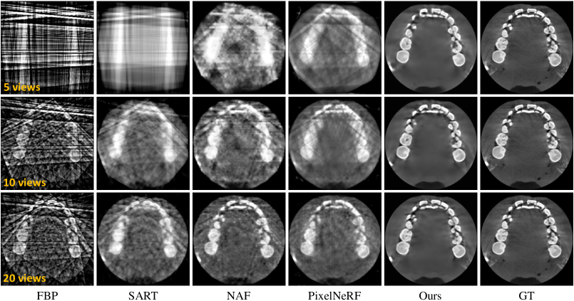
Figure 3: Qualitative comparison with different methods.

3.2 Results

3.2.1 Quantitative and Qualitative Results

Tab. 1 presents the quantitative comparisons of different methods. Our method outperforms all other methods by a significant margin in both PSNR and SSIM. Notably, our method achieves the highest performance with only 5 input views (27.38 dB of PSNR), and a PSNR above 30 dB for 20 input views, dramatically surpassing the current state-of-the-art method (i.e., NAF). Moreover, our reconstruction time is less than a second, which is much faster than other sparse-view methods (i.e., SART, NAF, and PixelNeRF). SART and NAF suffer from time-consuming iterative computation and per-scene optimization respectively, and we benefit from low-resolution feature querying compared to PixelNeRF.

In Fig. 3, we present a visual comparison of the reconstructed 3D CBCT images in axial slices. It can be seen that, FBP fails to handle sparse-view input, leading to severe streaking artifacts due to insufficient views. SART can significantly improve the quality by reducing those artifacts, but that trades off the important fine details. NAF is capable of high-quality reconstruction by adapting neural rendering with hash encoder. However, its quality drops drastically with extremely limited number of input views (e.g., 5, 10 views), as it is a per-scene optimized method without generalizable ability learned from a diverse data population. PixelNeRF also enjoys generalizable ability as we do, but it lacks volumetric supervision to ensure 3D quality, which is the crucial difference between medical imaging and natural scene. Notably, our method outperforms all other methods and is the only one that provides comparable quality with the ground truth, even with only 5 input views.

Table 2: Ablation study on different components.

Components				5 views		10 views		20 views
Baseline	ada.	$L_{proj}$	$L_{grad}$	PSNR	SSIM	PSNR	SSIM	PSNR	SSIM
$\checkmark$				26.47	0.88	27.86	0.90	29.97	0.93
$\checkmark$	$\checkmark$			26.98	0.89	28.57	0.91	30.85	0.94
$\checkmark$	$\checkmark$	$\checkmark$		27.18	0.89	28.70	0.91	31.02	0.94
$\checkmark$	$\checkmark$	$\checkmark$	$\checkmark$	27.38	0.89	28.81	0.92	31.34	0.94

3.2.2 Ablation Study

The quantitative ablation study results are listed in Table 2, where the baseline model simply makes use of average pooling to aggregate feature vectors from different input views and only adopts reconstruction and adversarial losses during training. Every $\checkmark$ in the table means adding the corresponding component into the baseline model as a new alternative solution. Note here, ’ada.’ in the table means adaptive feature fusing strategy. As can be seen, compared with other SOTA methods, our baseline already performs best. For example, in terms of PSNR, we gain remarkable $4.35$ dB, $3.83$ dB, and $3.12$ dB improvement for 5, 10, and 20 views against PixelNeRF. Because our strong baseline has equipped with geometry-aware view consistency in feature learning and voxel-wised supervision in training, which lay the foundation and are the keys to the success of our method. Furthermore, with the addition of other components, the PSNR and SSIM values increase gradually, which demonstrates the effectiveness of our technical designs. For example, adaptive feature fusing provides a more flexible and accurate integration of information from different views than average pooling, thus brings a relatively considerable improvement. While the projection loss boosts geometry-aware view consistency and the gradient loss enhances the sharpness, respectively.

3.2.3 Per-Scene Fine-Tuning

After across-scenes training, our model could provide a decent reconstructed CBCT image from sparse X-ray views. We could further fine-tune our result scene-wise by only making use of projection loss with the same input views. The PSNR value of reconstructed results would improve by 0.66 dB, 0.74 dB, and 0.75 dB on average for 5, 10, and 20 views after optimizing for about 4-15 minutes.

3.2.4 Application

We evaluate the quality of the reconstructed CBCT images by performing tooth segmentation as a downstream application. We first get expert manual annotations for each CBCT image in our testing set and use the pre-trained SOTA network [2] to segment teeth. As a reference, the average Dice score of the teeth segmentation from ground truth CBCT images (compared with human annotation) in our testing set is $0.94$. Thus, whichever method whose Dice score is closer to this value achieves a higher reconstruction quality. In Fig. 5, we report the Dice scores (mean and standard deviation) of all methods tested on CBCT images reconstructed with different numbers of input views. Note that, we omit some results in the figure (e.g., those from NAF with 5 and 10 views) that failed for tooth segmentation (i.e., Dice score less than 0.6) to ensure clear comparison. As can be seen, our method clearly outperforms all competitors indicating the usability and superior image quality of our reconstruction. Furthermore, we provide a visual example in Fig. 5, where our Dice scores are $0.88$, $0.90$, and $0.92$ for 5, 10, and 20 views, against $0.95$ of the ground truth CBCT segmentation for this specific case. Although our Dice scores are not as high as the ground truth, they are comparable indicating the great potential of our method for downstream applications and real clinical use.

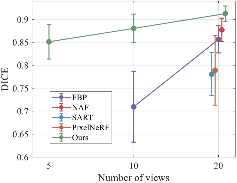
Figure 4: Quantitative comparison of tooth segmentation performance.

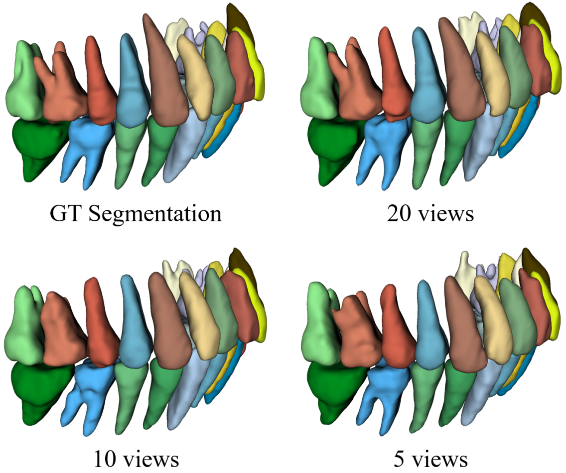
Figure 5: Qualitative results of tooth segmentation.

4 Conclusion

This paper proposes a novel attenuation field learning framework for sparse-view CBCT reconstruction. By learning the prior knowledge from the data population, our method can generalize to other patients without further training and efficiently solve the sparse-view input problem with high-quality reconstructed CBCT images. Extensive evaluations validate our superiority and the downstream application demonstrates the applicability of our method in real-world clinics.

References

- [1] Andersen, A., Kak, A.: Simultaneous algebraic reconstruction technique (sart): A superior implementation of the art algorithm. Ultrasonic imaging 6, 81–94 (02 1984). https://doi.org/10.1016/0161-7346(84)90008-7
- [2] Cui, Z., Fang, Y., Mei, L., Zhang, B., Yu, B., Liu, J., Jiang, C., Sun, Y., Ma, L., Jiawei, H., Liu, Y., Zhao, Y., Lian, C., Ding, Z., Zhu, M.: A fully automatic ai system for tooth and alveolar bone segmentation from cone-beam ct images. Nature Communications 13, 2096 (04 2022). https://doi.org/10.1038/s41467-022-29637-2
- [3] Feldkamp, L., Davis, L.C., Kress, J.: Practical cone-beam algorithm. J. Opt. Soc. Am 1, 612–619 (01 1984)
- [4] He, K., Zhang, X., Ren, S., Sun, J.: Deep residual learning for image recognition. 2016 IEEE Conference on Computer Vision and Pattern Recognition (CVPR) pp. 770–778 (2015)
- [5] Kasten, Y., Doktofsky, D., Kovler, I.: End-To-End Convolutional Neural Network for 3D Reconstruction of Knee Bones from Bi-planar X-Ray Images, pp. 123–133 (10 2020). https://doi.org/10.1007/978-3-030-61598-7_12
- [6] Ledig, C., Theis, L., Huszár, F., Caballero, J., Cunningham, A., Acosta, A., Aitken, A., Tejani, A., Totz, J., Wang, Z., Shi, W.: Photo-realistic single image super-resolution using a generative adversarial network. In: 2017 IEEE Conference on Computer Vision and Pattern Recognition (CVPR). pp. 105–114 (2017). https://doi.org/10.1109/CVPR.2017.19
- [7] Mao, X., Li, Q., Xie, H., Lau, R.Y., Wang, Z., Smolley, S.P.: Least squares generative adversarial networks. In: 2017 IEEE International Conference on Computer Vision (ICCV). pp. 2813–2821 (2017). https://doi.org/10.1109/ICCV.2017.304
- [8] Mildenhall, B., Srinivasan, P.P., Tancik, M., Barron, J.T., Ramamoorthi, R., Ng, R.: Nerf: Representing scenes as neural radiance fields for view synthesis. In: European Conference on Computer Vision (2020)
- [9] Müller, T., Evans, A., Schied, C., Keller, A.: Instant neural graphics primitives with a multiresolution hash encoding. ACM Transactions on Graphics (TOG) 41, 1 – 15 (2022)
- [10] Sanchez, I., Vilaplana, V.: Brain mri super-resolution using 3d generative adversarial networks (04 2018)
- [11] Shen, L., Zhao, W., Xing, L.: Patient-specific reconstruction of volumetric computed tomography images from a single projection view via deep learning. Nature biomedical engineering 3(11), 880—888 (November 2019). https://doi.org/10.1038/s41551-019-0466-4
- [12] Wang, Q., Wang, Z., Genova, K., Srinivasan, P., Zhou, H., Barron, J.T., Martin-Brualla, R., Snavely, N., Funkhouser, T.: Ibrnet: Learning multi-view image-based rendering. In: 2021 IEEE/CVF Conference on Computer Vision and Pattern Recognition (CVPR). pp. 4688–4697 (2021). https://doi.org/10.1109/CVPR46437.2021.00466
- [13] Wang, Z., Bovik, A., Sheikh, H., Simoncelli, E.: Image quality assessment: from error visibility to structural similarity. IEEE Transactions on Image Processing 13(4), 600–612 (2004). https://doi.org/10.1109/TIP.2003.819861
- [14] Ying, X., Guo, H., Ma, K., Wu, J., Weng, Z., Zheng, Y.: X2ct-gan: Reconstructing ct from biplanar x-rays with generative adversarial networks. In: 2019 IEEE/CVF Conference on Computer Vision and Pattern Recognition (CVPR). pp. 10611–10620 (2019). https://doi.org/10.1109/CVPR.2019.01087
- [15] Yu, A., Ye, V., Tancik, M., Kanazawa, A.: pixelnerf: Neural radiance fields from one or few images. 2021 IEEE/CVF Conference on Computer Vision and Pattern Recognition (CVPR) pp. 4576–4585 (2020)
- [16] Zha, R., Zhang, Y., Li, H.: NAF: Neural Attenuation Fields for Sparse-View CBCT Reconstruction, pp. 442–452 (09 2022). https://doi.org/10.1007/978-3-031-16446-0_42
- [17] Zhu, J.Y., Park, T., Isola, P., Efros, A.A.: Unpaired image-to-image translation using cycle-consistent adversarial networks. In: 2017 IEEE International Conference on Computer Vision (ICCV). pp. 2242–2251 (2017). https://doi.org/10.1109/ICCV.2017.244