Central exclusive diffractive $p$ $\bar{p}$ production in the Regge-eikonal model in the “scalar” proton approximation

Abstract

Central exclusive diffractive production(CEDP) of proton anti-proton pairs was calculated in the Regge-eikonal approach taking into account continuum and possible $f_{0}(2100)$ resonance. We use the simple model with the “scalar” proton. Data from ISR and STAR were analysed and compared with theoretical description. Some predictions for the LHC at 13 TeV are also presented. We discuss shortly possible nuances, problems and prospects of investigations of this process at present and future hadron colliders.

Introduction

As was often mentioned in the papers devoted to the process $p+p\to p+X+p$, low mass central exclusive diffractive production (LM CEDP) of resonances and di-hadron continua have a lot of advantages to study hadronic diffraction:

• LM CEDP is the tool for the investigation of hadronic resonances (like $f_{2}$ or $f_{0}$) and their decays to hadrons. We can extract different couplings of these resonances to reggeons (pomeron, Odderon etc) to understand their nature (structure and the interaction mechanisms).

• We can use LM CEDP to fix the procedure of calculations of “rescattering” (unitarity) corrections. For example, in the case of $p$ $\bar{p}$ production we have corrections in the initial proton-proton and final proton-proton and proton-anti-proton channels.

• Basic hadrons (pion, proton) are the most fundamental particles in the strong interactions, and LM CEDP gives us a powerful tool to go deep inside their properties, especially to investigate the form factor and scattering amplitudes for the off-shell (“virtual”) hadron.

• LM CEDP has rather large cross-sections. It is very important for an exclusive process, since in the special low luminocity runs (of the LHC) we need more time to get enough statistics.

• As was proposed in myCEDPpipiContinuum ,mySD , it is possible to extract some reggeon-hadron cross-sections. In the LM CEDP of the $p$ $\bar{p}$ we can analyze properties of the pomeron-pomeron to $p$ $\bar{p}$ exclusive cross-section.

• Diffractive patterns of CEDP processes are very sensitive to different approaches (subamplitudes, form factors, unitarization, reggeization procedure), especially differential cross-sections in $t$ and $\phi_{pp}$ (azimuthal angle between final protons), and also $M_{p\bar{p}}$ dependence. That is why these processes are used to verify different models of diffraction myCEDP1 ,myCEDP2 .

• Especially in the case of LM CEDP of $p$ $\bar{p}$ we have additional possibilities to investigate spin effects, helicity amplitudes, baryon trajectories, to search for Odderon and extract its coupling to proton.

• All the above items are additional advantages provided by the LM CEDP, which has usual properties of CEDP: clear signature with two final protons and two large rapidity gaps (LRG) LRG1 ,LRG2 and the possibility to use the “missing mass method” MMM .

Processes of the LM CEDP of di-hadrons were calculated in some works CEDPw1 -CEDPw6a which are devoted to most popular models. Authors have considered phenomenological, nonperturbative, perturbative and mixed approaches in Reggeon-Reggeon collision subprocess. Nuances of some approaches were analysed in the introduction of myCEDPpipiContinuum .

Recently in our works myCEDPpipiContinuum ,myCEDPpipiall we considered the LM CEDP with production of two pions. Here we consider other possible process, namely, LM CEDP of $p$ $\bar{p}$ system via resonance and continuum mechanisms. This process was also considered in CEDPw6a in the tensor pomeron model.

In this article we consider the case, depicted in Fig. 1, and compare the calculations against the data from ISR ISRdata1 -ISRdata3 , STAR STARdata3 -STARdata5 . Also we make predictions for the LHC.

In the first part of the present work we introduce the framework for calculations of di-baryon LM CEDP (kinematics, amplitudes, differential cross-sections) in the Regge-eikonal approach, wich was considered in details in myCEDPpipiContinuum ,myCEDPpipiall . Here we consider proton (anti-proton) as a “scalar”, that is why we can not calculate specific spin effects (like it was done in CEDPw6a ). Our goal at the present stage is to make preliminary estimations of some general distributions. Extension of the model to particles with any spin will be discussed in futher theoretical works. In this article calculation are almost similar to our works myCEDPpipiContinuum ,myCEDPpipiall with some modifications of the amplitudes.

In the second part we analyse the experimental data on the process at different energies and compare it with our pedictions.

To avoid complicated expressions in the main text, all the basic formulae are placed to Appendixes.

The purpose of this work is to give some hints and ideas to experimentalists of what we can expect in the LM CEDP of $p\bar{p}$: possible magnitudes of the couplings and cross-sections (from continuum and resonances), what is the difference between di-pion and other di-hadron production, how big could be spin effects, or contributions of secondary reggeons or Odderon and so on.

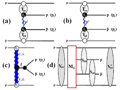
Figure 1: Amplitudes of the process of LM CEDP $p+p\to p+p\bar{p}+p$ in the Regge-eikonal approach for continuum (a),(b), LM CEDP of $f_{0}$ resonances (c) with subsequent decay to $p\bar{p}$. (a),(b): central part of the diagram is the continuum CEDP amplitude, where $T_{pp}$, $T_{p\bar{p}}$ are full elastic proton-proton(anti-proton) amplitudes, and the proton propagator depicted as dahsed zigzag line. (c): central part of the diagram contains pomeron-pomeron-resonance fusion with subsequent decay to $p\bar{p}$, propagator is taken in the Breit-Wigner approximation. Off-shell proton form factor on (a),(b) and other suppression form-factors (in the pomeron-pomeron-f or the $p\bar{p}f_{0}$) on (c) are presented as a black circles. Full unitarized amplitude (d) contains proton-proton rescatterings in the initial and final states, which are depicted as $V_{pp}$ and $V^{\prime}_{pp}$-blobes correspondingly, and proton-proton(anti-proton) rescattering corrections, which are also shown as $S_{pp,p\bar{p}}$-blobes.

1 General framework for calculations of LM CEDP

LM CEDP is the first exclusive two to four process which is driven basically by the pomeron-pomeron fusion subprocess. It serves as a clear process for investigations of resonances like $f_{0}$, $f_{2}$ and others with masses less than $5$ GeV. At the noment, for low central masses it is a huge problem to use perturbative approach, that is why we apply the Regge-eikonal method for all the calculations. For proton-proton and proton-anti-proton elastic amplitudes we use the model of godizovpp , godizovpip , which describe all the available experimental data on elastic scattering.

1.1 Components of the framework

LM CEDP process can be calculated in the following scheme (see Fig. 1):

1. We calculate the primary amplitudes of the processes, which are depicted as central parts of diagrams in Fig. 1. Here we consider the case, where the bare off-shell proton propagator in the amplitude for continuum $p\bar{p}$ production is taken in its simple form (without reggeization)

   $${\cal P}_{p}(\hat{t})=1/(\hat{t}-m_{p}^{2}),$$ (1)

   where $\hat{t}$ is the square of the momentum transfer between a pomeron and a proton in the pomeron-pomeron fusion process (see Appendix A for details).

   In the general case, which will be considered in future investigations, we have to do possible reggeization of the spinor proton with proton trajectory taken, for example, from protontraject1 :

   $$\alpha_{p}(\hat{t})=-0.4+0.9\hat{t}+0.125\hat{t}^{2}.$$

   As was noted at the beginning, here we consider the proton (anti-proton) as a “spin-0 particle”.

   Reggeization of the virtual proton propagator is not obvious, since the effect of this is expected to be small and moreover it is not even clear that we are in the relevant kinematic region ($|\hat{t}|\ll\hat{s}=M_{p\bar{p}}^{2}$) to include such corrections for central production. It was verified also in the calculations presented in this paper. For example, we can use the replacement

   $$\frac{1}{\hat{t}-m_{p}^{2}}\to\frac{\mathrm{e}^{\alpha_{p}(\hat{t})|\Delta Y|}}{\hat{t}-m_{p}^{2}},$$ (2)

   as was done in CEDPw1 -CEDPw3 . This expression gives correct “reggeized” behaviour in the relevant kinematical region, and the usual “bare” proton propagator behaviour for small difference between rapidities of the final central proton (anti-proton). As to authors of CEDPw4 -CEDPw5a , we could use phenomenological expression for virtual proton propagator like (see (3.25), (3.26) of CEDPw5a for the pion propagator)

   $$\frac{1}{\hat{t}-m_{p}^{2}}F(\Delta Y)+(1-F(\Delta Y)){\cal P}_{p}(\hat{s},\hat{t}),$$

   $$F(\Delta Y)=\mathrm{e}^{-c_{y}\Delta Y},\,\Delta Y=y_{p}-y_{\bar{p}},$$ (3)

   to take into accound possible non-Regge behaviour for $\hat{t}\sim\hat{s}/2$, i.e. for small rapidity separation $\Delta Y$ between final proton and anti-proton. The Regge model really does not work in this area or it needs to be modified (as was done, for example, in works CEDPw4 -CEDPw6 , with empirical formulae or additional assumptions).

   We use also full eikonalized expressions for proton-proton and proton-anti-proton amplitudes, which can be found in the Appendix B.

2. After the calculation of the primary LM CEDP amplitudes we have to take into account all possible corrections in proton-proton and proton-anti-proton elastic channels due to the unitarization procedure (so called “soft survival probability” or “rescattering corrections”), which are depicted as $V_{pp}$, $V^{\prime}_{pp}$ and $S_{pp,p\bar{p}}$ blobes in Fig. 1. For proton-proton and proton-anti-proton elastic amplitudes we use the model of godizovpp , godizovpip (see Appendix B). Possible final interaction between hadrons of the central system is not shown in Fig. 1, since we neglect it in the present calculations.

In this article we do not consider so called “enhanced” corrections CEDPw1 -CEDPw3 , since they give nonleading contributions in our model due to smallness of the triple pomeron vertex. Also we have no possible absorptive corrections inside the $p\bar{p}$ central system, since the central mass is low, and also there is a lack of data on this process to define parameters of the model.

Exact kinematics of the two to four process for our case is outlined in Appendix A.

Here we use the model, presented in Appendix B for example. You can use another one, which is proved to describe well all the available data on proton-proton and proton-anti-proton elastic processes.

1.2 Continuum $p\bar{p}$ production

Final expression for the amplitude for the continuum $p\bar{p}$ production with initial proton-proton and final proton-(anti-)proton “rescattering” corrections (see Fig. 1 (a), (b)) can be written as

$$M^{U}\left(\{p\}\right)=$$

$$=\int\int\frac{d^{2}\vec{q}}{(2\pi)^{2}}\frac{d^{2}\vec{q}^{\prime}}{(2\pi)^{2}}\frac{d^{2}\vec{q}_{1}}{(2\pi)^{2}}\frac{d^{2}\vec{q}_{2}}{(2\pi)^{2}}V_{pp}(s,q^{2})V_{pp}(s^{\prime},q^{\prime 2})$$

$$\times\;\left[S_{p\bar{p}}(\tilde{s}_{14},q_{1}^{2})M_{0}\left(\{\tilde{p}\}\right)S_{pp}(\tilde{s}_{23},q_{2}^{2})+(3\leftrightarrow 4)\right]$$ (4)

$$M_{0}\left(\{p\}\right)=\phantom{I^{2^{2^{2}}}}$$

$$=T^{el}_{pp}(s_{13},t_{1}){\cal P}_{p}(\hat{t})\left[\hat{F}_{p}\left(\hat{t}\right)\right]^{2}T^{el}_{p\bar{p}}(s_{24},t_{2}),$$ (5)

where functions are defined in (30)-(31) of Appendix B, and sets of vectors are

$$\{p\}\equiv\{p_{a},p_{b},p_{1},p_{2},p_{3},p_{4}\}$$ (6)

$$\{\tilde{p}\}\equiv\{p_{a}-q,p_{b}+q;p_{1}+q^{\prime}+q_{1},$$

$$\;\;\;\;\;\;\;\;\;\;\;\;p_{2}-q^{\prime}+q_{2},p_{3}-q_{2},p_{4}-q_{1}\},$$ (7)

and

$$\tilde{s}_{14} = \left(p_{1}+p_{4}+q^{\prime}\right)^{2},\;\tilde{s}_{23}=\left(p_{2}+p_{3}-q^{\prime}\right)^{2},$$ (8)

$$s_{ij} = \left(p_{i}+p_{j}\right)^{2},\;t_{1,2}=\left(p_{a,b}-p_{1,2}\right)^{2},$$ (9)

$$\hat{s} = \left(p_{3}+p_{4}\right)^{2},\;\hat{t}=\left(p_{a}-p_{1}-p_{3}\right)^{2}$$ (10)

Off-shell proton form factor is equal to unity on mass shell $\hat{t}=m_{p}^{2}$ and taken as exponential

$$\hat{F}_{p}=\mathrm{e}^{(\hat{t}-m_{p}^{2})/\Lambda_{p}^{2}},$$ (11)

where $\Lambda_{p}\sim 1$ GeV is taken from the fits to LM CEDP of $p\bar{p}$ at low energies (see next section). In this paper we use only exponential form, but it is possible to use other parametrizations (see CEDPw6a ).

Other functions are defined in Appendix B. Then we can use the expression (23) to calculate the differential cross-section of the process.

1.3 CEDP of low mass resonances.

Here we consider, for example, only one $f_{0}$ resonance, say, $f_{0}(2100)$, just to see the final picture and possible changes in the diffractive patterns. The general unitarized amplitude (see Fig. 1(c)) is similar to the expression (4), where amplitude $M_{0}\left(\{p\}\right)$ is replaced by the corresponding central primary amplitude for the resonance production and futher decay to $p\bar{p}$.

For the $f_{0}(2100)$ meson amplitude is constructed from the proton-Pomeron form-factor, pomeron-Pomeron coupling to the meson, the off-shell propagator, the off-shell form-factor and the decay vertice.

The primary amplitude is given in the Appendix C.

1.4 Nuances of calculations.

In the next section one can see that there are some difficulties in the data fitting. In this subsection let us discuss some nuances of calculations, which could change the situation.

We have to pay special attention to amplitudes, where one or more external particles are off their mass shell. The example of such an amplitude is the proton-(anti-)proton one $T_{pp}$ ($T_{p\bar{p}}$), which is the part of the CEDP amplitude (see (4)). For this amplitude in the present paper we use Regge-eikonal model with the eikonal function in the classical Regge form. And “off-shell” condition for one of the baryons is taken into account by additional phenomenological form factor $\hat{F}_{p}(\hat{t})$. But there are at least two other possibilities.

The first one was considered in PetrovOffshell . For amplitude with one particle off-shell the formula

$$T^{*}(s,b)=\frac{\delta^{*}(s,b)}{\delta(s,b)}T(s,b)=\frac{\delta^{*}(s,b)}{\delta(s,b)}\frac{\mathrm{e}^{2\mathrm{i}\delta(s,b)}-1}{2\mathrm{i}}$$ (12)

was used. In our case

$$\delta(s,b)=\delta_{pp,p\bar{p}}(s,b;m_{p}^{2},m_{p}^{2},m_{p}^{2},m_{p}^{2}),$$

$$\delta^{*}(s,b)=\delta_{pp,p\bar{p}}^{*}(s,b;\hat{t},m_{p}^{2},m_{p}^{2},m_{p}^{2})$$

$$\left.\delta_{pp,p\bar{p}}=\delta^{*}_{pp,p\bar{p}}\right|_{\hat{t}\to m_{p}^{2}}.$$ (13)

$\delta_{pp,p\bar{p}}$ is the eikonal function (see (28)). This is similar to the introduction of the additional form factor, but in a more consistent way, which takes into account the unitarity condition.

The second one arises from the covariant reggeization method, which was considered in the Appendix C of myCEDPpipiContinuum . For the case of conserved hadronic currents we have definite structure in the Legendre function, which is transformed in a natural way to the case of the off-shell amplitude. But in this case off-shell amplitude has a specific behaviour at low t values (see myCEDP2 for details). As was shown in myCEDP2 , unitarity corrections can mask this behavior. Also in this case we have to take into account the spinor nature of the proton and modify the covariant reggeization approach presented in  myCEDPpipiContinuum .

2 Data from hadron colliders versus results of calculations

Our basic task is to extract the fundamental information on the interaction of hadrons from different cross-sections (“diffractive patterns”):

• from t-distributions we can obtain size and shape of the interaction region;

• the distribution on the azimuthal angle between final protons gives quantum numbers of the produced system (see myCEDP2 ,myWA102 and references therein);

• from $M_{c}$ (here $M_{c}=M_{p\bar{p}}$) dependence and its influence on t-dependence we can make some conclusions about the interaction at different space-time scales and interrelation between them. Also we can extract couplings of reggeons to different resonances.

Process $p+p\to p+p\bar{p}+p$ is one of the basic “standard candles”, which we can use to estimate other CEDP processes. In this section we consider the available experimental data on the process and make an attempt to extract the information on couplings and form-factors.

a)

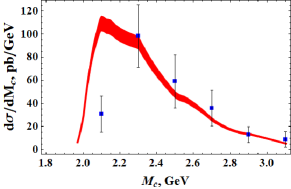
b)

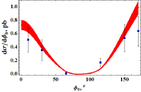
c)

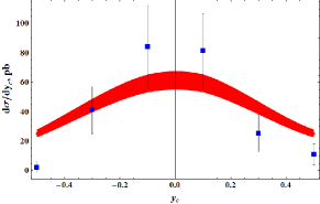
d)

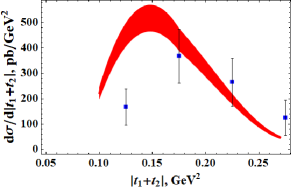
Figure 2: The new data on the process $p+p\to p+p\bar{p}+p$ at $\sqrt{s}=200$ GeV (STAR collaboration STARdata3 -STARdata5 ): $|\eta_{p,\bar{p}}|<0.7$, $p^{p}_{T}(p^{\bar{p}}_{T})>0.4$ GeV, $\min(p^{p}_{T},p^{\bar{p}}_{T})<1.1$ GeV, $p_{x}>-0.2$ GeV, $0.2$ GeV$<|p_{y}|<0.4$ GeV, $(p_{x}+0.3\,\mathrm{GeV})^{2}+p_{y}^{2}<0.25$ GeV², where $p$ denotes the momenta of final forward protons. Curves correspond to $\Lambda_{p}=1.12$ GeV in the off-shell proton form factor (11) and pomeron-pomeron-$f_{0}(2100)$ coupling is equal to $0.64$. Curves correspond to the sum of all amplitudes. Thickness of the curves shows the errors of numerical Monte-carlo calculations. Additional interpolation was used between calculated points for smoothing.

2.1 STAR data versus the model distributions

In this subsection the data from the STAR collaboration STARdata3 -STARdata5 and model curves for all the cases of Fig. 1 are presented. In our approach we have two free parameters: $\Lambda_{p}$ (for the continuum) and the coupling of $f_{0}(2100)$ to pomeron $g_{\mathbb{PP}f}$, which we can extract from the data or fix from some model assumptions. All the distributions are depicted for $\Lambda_{p}=1.12$ GeV. Here we take only $f_{0}(2100)$ resonance with pomeron-pomeron-$f_{0}(2100)$ coupling is equal to $0.64$ (this value is inspired by the paper on possible “glueball” states GodizovResonances ).

As you can see from the Fig. 2, we can describe the data rather well. From these data we fix the parameter $\Lambda_{p}=1.12$ GeV, and then we can make some predictions for other energies. Valuable difference is seen only in the region of small central masses and small $|t_{1}+t_{2}|$.

And on the Fig. 3 we see predictions for the STAR data at $\sqrt{s}=510$ GeV. For the normalized cross-section we see good description of the distribution shape. Unfortunately, from this data we can not make any conclusions on the absolute value of the cross-section versus predictions, since for now there are no official publications on the integrated luminosity in this case. So, more correct comparison is postponed for further publications.

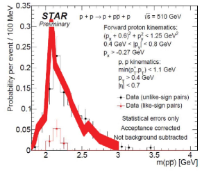
Figure 3: (a) The new data (normalized cross-section) on the process $p+p\to p+p\bar{p}+p$ at $\sqrt{s}=510$ GeV (STAR collaboration STARdata5 ): $|\eta_{p,\bar{p}}|<0.7$, $p^{p}_{T}(p^{\bar{p}}_{T})>0.4$ GeV, $\min(p^{p}_{T},p^{\bar{p}}_{T})<1.1$ GeV, $p_{x}>-0.27$ GeV, $0.4$ GeV$<|p_{y}|<0.8$ GeV, $(p_{x}+0.6\,\mathrm{GeV})^{2}+p_{y}^{2}<1.25$ GeV², where $p$ denotes the momenta of final forward protons. Curves correspond to $\Lambda_{p}=1.12$ GeV in the off-shell proton form factor (11) and pomeron-pomeron-$f_{0}(2100)$ coupling is equal to $0.64$. Thick solid curve corresponds to the sum of all amplitudes, thickness of the curves shows the errors of numerical calculations.

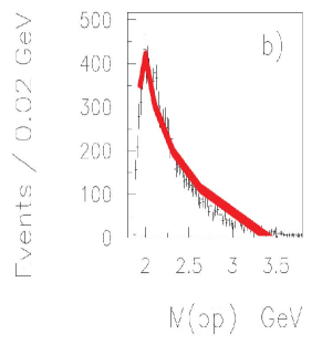
Figure 4: The data on the process $p+p\to p+p\bar{p}+p$ (WA102 collaboration ISRdata1 ): at $\sqrt{s}=29.1$ GeV, $|p^{c}_{x}|<14$ GeV,$|p^{c}_{y}|<0.16$ GeV,$|p^{c}_{z}|<0.08$ GeV, $\xi_{1,2\,p}>0.8$. Theoretical curves, multiplied by 740, correspond to $\Lambda_{p}=1.12$ GeV in the off-shell proton form factor (11) and pomeron-pomeron-$f_{0}(2100)$ coupling is equal to $0.64$. Solid curve corresponds to the sum of all amplitudes, thickness of the curve shows the errors of numerical calculations.

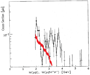
Figure 5: The data (black circles) on the process $p+p\to p+p\bar{p}+p$ (ABCDHW collaboration ISRdata2 ) at $\sqrt{s}=62$ GeV, $\xi_{1,2\,p}>0.9$, $|y_{p,\bar{p}}|<1.5$, $|t_{1,2}|>0.08$ GeV². Theoretical curves, multiplied by 200, correspond to $\Lambda_{p}=1.12$ GeV in the off-shell proton form factor (11) and pomeron-pomeron-$f_{0}(2100)$ coupling is equal to $0.64$. Solid curve corresponds to the sum of all amplitudes, thickness of the curve shows the errors of numerical calculations.

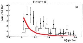
Figure 6: The data on the process $p+p\to p+p\bar{p}+p$ (AFS collaboration ISRdata3 ) at $\sqrt{s}=63$ GeV, $\xi_{1,2\,p}>0.95$, $|y_{p,\bar{p}}|<1$, $0.01$ GeV${}^{2}<|t_{1,2}|<0.06$ GeV². Theoretical curves correspond to $\Lambda_{p}=1.12$ GeV in the off-shell proton form factor (11) and pomeron-pomeron-$f_{0}(2100)$ coupling is equal to $0.64$. Solid curve corresponds to the sum of all amplitudes, thickness of the curve shows the errors of numerical calculations. $\sigma_{exp}=2.5\pm 1.25$ nb was calculated from $d\sigma/dt_{1}dt_{2}\sim 1\pm 0.5\;\mu$b GeV^-4 (see text).

2.2 Low energy data versus model cases

If we take a look at the low energy data, we can discover several significant contradictions similar to those found in the production of two pions myCEDPpipiall . This is obvious if we use the data of the WA102 collaboration ISRdata1 at $\sqrt{s}=29.1$ GeV (see Fig. 4). The figure shows that the shape of the predicted distribution is close to the experimental one, but the discrepancy by a factor of 720 (integrated cross-section is about 260 pb, and in ISRdata1 we have 186 nb) indicates that the approach used in this energy range fails, and we must take into account other mechanisms for the CEDP of proton-antiproton pairs. It is possible that resonant production plays a key role here, as was pointed out earlier CEDPw6a , especially at low masses of the central system. Also, at low energies, spin effects play a significant role, although their contribution will most likely give an increase of no more than $\sim 2$ times.

The situation is almost the same, when we try to compare predictions with the data from ABCDHW collaboration ISRdata2 at $\sqrt{s}=62$ GeV (see Fig. 5). The quality of the data is not so good, errors are large. Experimental integrated cross-section in this case is 0.8$\pm$0.17 $\mu$b, and predictions give only 0.002 $\mu$b, i.e. about 400 times lower. In this case $|t_{1,2}|>0.08$ GeV², and this cut removes the region which gives the major contribution to the cross-section. We see the similar discrepancy in CEDPw6a , when one takes into account rescattering corrections.

A more interesting situation arises when we take the data from the AFS collaboration ISRdata3 . From this paper we take differential cross sections

$$\left.d\sigma/dt_{1}dt_{2}\right|_{t_{1,2}=-0.035\;\rm{GeV}^{2}}=1.0\pm 0.5\;\mu\rm{b}\;\rm{GeV}^{-4}.$$ (14)

If we use a simple form $A\times\rm{e}^{B(t_{1}+t_{2})}$ for the differential cross-section in a very wide range of B from 3 GeV^-2 up to 12 GeV^-2, we can find for the integrated cross-section

$$\sigma_{exp}\simeq 2.5\pm 1.25\;\rm{nb}.$$ (15)

Theoretical calculations give

$$\left.d\sigma/dt_{1}dt_{2}\right|_{t_{1,2}=-0.035\;\rm{GeV}^{2}}=0.3\;\mu\rm{b}\;\rm{GeV}^{-4},$$ (16)

$$\sigma_{th}=1.9\;\rm{nb}.$$ (17)

Also in the Fig. 6 we can see, that the curve has no such a huge discrepancy with the experimental points as in two previous cases. The discrepancy is of the same order and even less than it was in myCEDPpipiall for the di-pion production at the ISR.

We can conclude, that the model is failed to describe the low energy data, if we fix parameters from the STAR data. For these low energies we have to take into account other mechanisms for the CEDP of $p\bar{p}$. Resonant production may play a key role. Also these mechanisms may include possible corrections to proton-proton(anti-proton) amplitudes at low energies, since our approach describe data well only for energies greater than $\sim 10$ GeV. And in each $T_{pp,p\bar{p}}$ amplitude in Fig. 1 (a),(b) the energy can be even less than $5$ GeV. In the present calculations, just to check preliminary and qualitatively the effect of secondary reggeons at very low energy and to improve the situation, we use simple exponential parametrization (Born approximation with secondary reggeons) for $T_{pp,p\bar{p}}$ elastic amplitude to cover the energy value down to the threshold $\sim 2$ GeV.

2.3 Predictions for LHC

a)

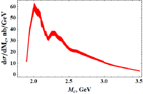
Figure 7: Predictions for CMS energies on the process $p+\bar{p}\to p+p\bar{p}+\bar{p}$ are shown for $\sqrt{s}=13$ TeV with cuts $|\eta_{p,\bar{p}}|<2.4$, $p_{T,p,\bar{p}}>0.2$ GeV. Theoretical curves correspond to $\Lambda_{p}=1.12$ GeV in the off-shell proton form factor (11) and pomeron-pomeron-$f_{0}(2100)$ coupling is equal to $0.64$. Solid curve correspond to the sum of all amplitudes, thickness of the curve shows the errors of numerical calculations.

In Fig. 7 one can see the prediction for the LHC at 13 TeV for the process, that corresponds to the parameter $\Lambda_{p}=1.12$ GeV, which better fits the STAR data on the Fig. 2. The integrated cross-section for these kinematical cuts is about 35 nb, which is about three orders of magnitude smaller than the cross section of di-pion CEDP. The number of $\pi^{+}\pi^{-}$ CEDP events is of the order $10^{4}$ for the LHC at the integrated luminosity $\sim 200\div 500\;\mu$b^-1, which is enough to obtain precise distributions in the central mass. That is why for the CEDP of $p\bar{p}$ we should have at least $\sim 50\div 100$ nb^-1 integrated luminosity for our investigations.

Summary and conclusions

To conclude this article, we can summarize the above analysis in a few statements:

1. the result is crucially dependent on the choice of $\Lambda_{p}$ in the off-shell proton form factor, i.e. on $\hat{t}$ (virtuality of the proton) dependence. This dependance is more significant than in the CEDP of di-pions. In the present approach we take $\Lambda_{p}=1.12$ GeV and couplings:

   $$g_{\mathbb{PP}f_{0}(2100)} = 0.64,$$

   $$g_{p\bar{p}f_{0}(2100)} = 3.1,$$ (18)

   The coupling of pomeron to $f_{0}(2100)$ is taken as in GodizovResonances just for tests.

2. if we try to fit the data from STAR STARdata3 -STARdata5 , we can fix the parameter $\Lambda_{p}=1.12$ GeV, for which the description is quite good.

3. for the ISR energies the situation is quite contradictory:

   • at $\sqrt{s}=29$ GeV we observe a difference of almost three orders of magnitude (although the shape of the theoretical and experimental distributions is the same);

   • at $\sqrt{s}=62$ GeV, when $|t_{1,2}|>0.08\;\rm{GeV}^{2}$, the difference is already of the order of 200;

   • at $\sqrt{s}=63$ GeV, for

     $0.01\;\rm{GeV}^{2}<|t_{1,2}|<0.06\;\rm{GeV}^{2}$,

     the predictions turn out to be only about 2 times smaller.

   This has to be explained somehow. We can assume that additional resonant production plays a key role, spin effects at low energy are rather big, contributions from other processes ($\gamma\gamma\to p\bar{p}$, $\gamma\mathbb{O}\to p\bar{p}$, single and double dissociation) must also be taken into account. There are also effects related to the irrelevance and possible modifications of the Regge approach (for the virtual proton exchange) in this kinematical region, corrections to $T_{pp,p\bar{p}}(s,t)$ for$\sqrt{s}<5$ GeV, corrections to proton-anti-proton scattering at low $M_{p\bar{p}}$;

4. Based on the predictions for $\sqrt{s}=13$ TeV, we can say that in order to study this process at the LHC, we need a minimum integrated luminosity of the order of $\sim 50\div 100$ nb^-1.

In further works we will take into account possible modifications of the model (proton-anti-proton low energy cross-section, additional off-shell effects in subamplitudes, spin effects, contributions from dissociative processes and so on) for best description of the data. This model will be implemented to the new version of the Monte-carlo event generator ExDiff ExDiffmanual . It is possible to calculate LM CEDP for other di-hadron final states ($\phi\phi$, $K^{+}K^{-}$, $\eta\eta^{\prime}$ etc.), which are also very informative for our understanding of diffractive mechanisms in strong interactions.

Appendix A. Kinematics of LM CEDP

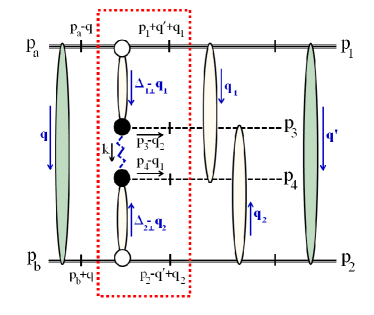
Figure 8: Total amplitude of the process of di-hadron LM CEDP $p+p\to p+h\bar{h}+p$ with detailed kinematics. Proton-proton rescatterings in the initial and final states are depicted as black blobes, and hadron-proton subamplitudes are also shown as shaded blobes. All momenta are shown. Basic part of the amplitude, $M_{0}$ (see eq. (5)), without corrections is circled by a dotted line. Crossed lines are on mass shell. Here $\Delta_{1\perp}=\Delta_{1}-q-q^{\prime}$, $\Delta_{2\perp}=\Delta_{2}+q+q^{\prime}$, $\hat{t}=k^{2}=(\Delta_{1\perp}-q_{1}-p_{3}+q_{2})^{2}$, $\hat{u}=(\Delta_{1\perp}-q_{1}-p_{4})^{2}$, $\hat{s}=(p_{3}+p_{4}-q_{1}-q_{2})^{2}$.

The $2\to 4$ process $p(p_{a})+p(p_{b})\to p(p_{1})+p(p_{3})+\bar{p}(p_{4})+p(p_{2})$ can be described as follows (the notation for any momentum is $k=(k_{0},k_{z};\vec{k})$, $\vec{k}=(k_{x},k_{y})$):

$$p_{a} = \left(\frac{\sqrt{s}}{2},\beta\frac{\sqrt{s}}{2};\vec{0}\right),\;p_{b}=\left(\frac{\sqrt{s}}{2},-\beta\frac{\sqrt{s}}{2};\vec{0}\right),$$

$$p_{1,2} = \left(E_{1,2},p_{1,2z};\vec{p}_{1,2\perp}\right),E_{1,2}=\sqrt{p_{1,2z}^{2}+\vec{p}_{1,2\perp}^{2}+m_{p}^{2}},\;$$

$$p_{3,4} = \left(m_{3,4\perp}\mathrm{ch}\;y_{3,4},m_{3,4\perp}\mathrm{sh}\;y_{3,4};\vec{p}_{3,4\perp}\right)=$$

$$= \left(\sqrt{m_{p}^{2}+\vec{p}_{3,4\perp}^{2}\mathrm{ch}^{2}\eta_{3,4}},|\vec{p}_{3,4\perp}|\;\mathrm{sh}\;\eta_{3,4};\vec{p}_{3,4\perp}\right),$$

$$m_{i\perp}^{2} = m_{i}^{2}+\vec{p}_{i\perp}^{2},\;m_{1,2}=m_{p},\;m_{3,4}=m_{h},$$

$$\vec{p}_{4\perp} = -\vec{p}_{3\perp}-\vec{p}_{1\perp}-\vec{p}_{2\perp},\;$$

$$\beta = \sqrt{1-\frac{4m_{p}^{2}}{s}},\;s=(p_{a}+p_{b})^{2},\;s^{\prime}=(p_{1}+p_{2})^{2}.$$ (19)

Here $y_{i}$ ($\eta_{i}$) are rapidities (pseudorapidities) of final hadrons.

Phase space of the process in terms of the above variables is the following

$$d\mathrm{\Phi}_{2\to 4} = \left(2\pi\right)^{4}\delta^{4}\left(p_{a}+p_{b}-\sum_{i=1}^{4}p_{i}\right)\prod_{i=1}^{4}\frac{d^{3}p_{i}}{(2\pi)^{3}2E_{i}}=$$

$$= \frac{1}{2^{4}(2\pi)^{8}}\prod_{i=1}^{3}p_{i\perp}dp_{i\perp}d\phi_{i}\cdot dy_{3}dy_{4}\cdot{\cal J};$$

$${\cal J} = \frac{dp_{1z}}{E_{1}}\frac{dp_{2z}}{E_{2}}\delta\left(\sqrt{s}-\sum_{i=1}^{4}E_{i}\right)\delta\left(\sum_{i=1}^{4}p_{iz}\right)=$$ (20)

$$= \frac{1}{\left|\tilde{E}_{2}\tilde{p}_{1z}-\tilde{E}_{1}\tilde{p}_{2z}\right|},$$

where $p_{i\perp}=\left|\vec{p}_{i}\right|$, $\tilde{p}_{1,2z}$ are appropriate roots of the system

$$\begin{cases}&A=\sqrt{s}-E_{3}-E_{4}=\sqrt{m_{1\perp}^{2}+p_{1z}^{2}}+\sqrt{m_{2\perp}^{2}+p_{2z}^{2}},\\ &B=-p_{3z}-p_{4z}=p_{1z}+p_{2z},\end{cases}$$ (21)

$$\tilde{p}_{1z} = \frac{B}{2}+\frac{1}{2(A^{2}-B^{2})}\left[B\left(m_{1\perp}^{2}-m_{2\perp}^{2}\right)+A\cdot\lambda_{0}^{1/2}\right],$$

$$\lambda_{0} = \lambda\left(A^{2}-B^{2},m_{1\perp}^{2},m_{2\perp}^{2}\right).$$ (22)

Here $\lambda(x,y,z)=x^{2}+y^{2}+z^{2}-2xy-2xz-2yz$, and then ${\cal J}^{-1}=\lambda_{0}^{1/2}/2$.

For the differential cross-section we have

$$\frac{d\sigma_{2\to 4}}{\prod_{i=1}^{3\phantom{I}}dp_{i\perp}d\phi_{i}\cdot dy_{3}dy_{4}} = \frac{1}{2\beta s}\cdot\frac{\prod_{i=1}^{3}p_{i\perp}}{2^{4}(2\pi)^{8}\cdot\frac{1}{2}\lambda_{0}^{1/2}}\left|T\right|^{2}=$$ (23)

$$= \frac{\prod_{i=1}^{3}p_{i\perp}}{2^{12}\pi^{8}\beta s\lambda_{0}^{1/2}}\left|T\right|^{2}.$$

Pseudorapidity is more convenient experimental variable, and we can use the transform

$$\frac{dy_{i}}{d\eta_{i}}=\frac{p_{i\perp}\mathrm{ch}\eta_{i}}{\sqrt{m_{i}^{2}+p_{i\perp}^{2}\mathrm{ch}^{2}\eta_{i}}}$$ (24)

to get the differential cross-section in pseudorapidities.

In some cases it is convenient to use other variables for the integration of the cross-section and calculation of distributions on central mass. For these cases we have:

$$d\mathrm{\Phi}_{2\to 4} = \frac{1}{2^{4}(2\pi)^{8}}\prod_{i=1}^{2}dt_{i}d\phi_{i}\cdot M_{c}dM_{c}d\eta_{c}dc^{*}d\phi^{*}\cdot{\cal J}^{\prime};$$

$${\cal J}^{\prime} = \frac{\beta_{M}}{4\beta_{1}\beta_{2}s}\frac{dy_{c}}{d\eta_{c}},\,\,\,\,\,\beta_{i}\simeq\sqrt{1+\frac{4(m_{p}^{2}-(1-\xi_{i})t_{i})}{\beta^{2}s^{2}(1-\xi_{i})^{2}}};$$

$$\beta_{M} = \sqrt{1-\frac{4m_{p}^{2}}{M_{c}^{2}}},\,\,\frac{dy_{c}}{d\eta_{c}}=\frac{p_{c\perp}\mathrm{ch}\eta_{c}}{\sqrt{M_{c}^{2}+p_{c\perp}^{2}\mathrm{ch}^{2}\eta_{c}}};$$ (25)

$$\frac{d\sigma_{2\to 4}}{\prod_{i=1}^{2\phantom{I}}dt_{i}d\phi_{i}dM_{c}d\eta_{c}dc^{*}d\phi^{*}} = \frac{1}{2\beta s}\cdot\frac{M_{c}\beta_{M}\frac{dy_{c}}{d\eta_{c}}}{2^{4}(2\pi)^{8}\cdot 4\beta_{1}\beta_{2}s}\left|T\right|^{2}$$ (26)

$$= \frac{M_{c}\beta_{M}\frac{dy_{c}}{d\eta_{c}}}{2^{15}\pi^{8}\beta\beta_{1}\beta_{2}s^{2}}\left|T\right|^{2},$$

where $c^{*}=\cos\theta^{*}$, $\theta^{*}$ and $\phi^{*}$ are polar and azimuthal angles of the central hadron momenta in the $h\bar{h}$ rest frame, $M_{c}$ is the di-hadron mass, $\eta_{c}$ is the di-hadron pseudorapidity, $t_{1}=(p_{a}-p_{1})^{2}$, $t_{2}=(p_{b}-p_{2})^{2}$ and

$$\xi_{1,2}\simeq\sqrt{\frac{M_{c}^{2}-t_{1}-t_{2}+2\sqrt{t_{1}t_{2}}\cos(\phi_{1}-\phi_{2})}{s}}\mbox{\bf e}^{\pm y_{c}}.$$

For exact calculations of elastic subprocesses (see Fig. 8) of the type
$a(p_{1})+b(p_{2})\to c(p_{1}-q_{el})+d(p_{2}+q_{el})$:

$$q_{el} = \left(q_{0},q_{z};\vec{q}\right),$$

$$q_{z} = -\frac{b}{2a}\left(1-\sqrt{1-\frac{4ac}{b^{2}}}\right),$$

$$q_{0} = \frac{A_{0}q_{z}+\vec{p}_{1\perp}\vec{q}+\vec{p}_{2\perp}\vec{q}}{A_{z}},$$

$$a = A_{z}^{2}-A_{0}^{2},\;b=-2\left(A_{z}\cdot{\cal D}+A_{0}\left(\vec{p}_{1\perp}\vec{q}+\vec{p}_{2\perp}\vec{q}\right)\right),$$

$$c = 2A_{z}B_{z}-\left(\vec{p}_{1\perp}\vec{q}+\vec{p}_{2\perp}\vec{q}\right)^{2}+\vec{q}^{2}A_{z}^{2},$$

$$A_{0} = p_{1z}+p_{2z},\;A_{z}=p_{10}+p_{20},$$

$$B_{0} = p_{1z}\cdot\vec{p}_{2\perp}\vec{q}-p_{2z}\cdot\vec{p}_{1\perp}\vec{q},$$

$$B_{z} = p_{10}\cdot\vec{p}_{2\perp}\vec{q}-p_{20}\cdot\vec{p}_{1\perp}\vec{q},$$

$${\cal D} = p_{1z}p_{20}-p_{2z}p_{10},$$ (27)

and $q_{el}^{2}\simeq-\vec{q}^{2}$.

Appendix B. Regge-eikonal model for elastic proton-proton and proton-anti-proton scattering

Here is a short review of formulae for the Regge-eikonal approach godizovpp , godizovpip , which we use to estimate rescattering corrections in the proton proton and pion proton channels.

Amplitudes of elastic proton-proton and proton-anti-proton scattering are expressed in terms of eikonal functions

$$T_{pp,p\bar{p}}^{el}(s,b) = \frac{\mathrm{e}^{-2\Omega_{pp,p\bar{p}}^{el}(s,b)}-1}{2\mathrm{i}},$$

$$\Omega_{pp,p\bar{p}}^{el}(s,b) = -\mathrm{i}\,\delta_{pp,p\bar{p}}^{el}(s,b),$$

$$\delta^{el}_{pp,p\bar{p}}(s,b) = \frac{1}{16\pi s}\int_{0}^{\infty}d(-t)J_{0}(b\sqrt{-t})\delta^{el}_{pp,p\bar{p}}(s,t).,$$ (28)

$$\delta^{el}_{pp,p\bar{p}}(s,t) \simeq$$

$$\!\!\!\!\!\!\!\!g_{pp\mathbb{P}}(t)^{2} \!\!\!\!\!\!\!\!\left(\mathrm{i}+\tan\frac{\pi(\alpha_{\mathbb{P}}(t)-1)}{2})\right)\pi\alpha^{\prime}_{\mathbb{P}}(t)\left(\frac{s}{2s_{0}}\right)^{\alpha_{\mathbb{P}}(t)},$$

$$\alpha_{\mathbb{P}}(t) = 1+\frac{\alpha_{\mathbb{P}}(0)-1}{1-\frac{t}{\tau_{a}}}\,,\,g_{pp\mathbb{P}}(t)=\frac{g_{pp\mathbb{P}}(0)}{\left(1-a_{g}t\right)^{2}}.$$ (29)

Here we use only pomeron contribution for the sake of simplicity, that is why we can not analyse possible difference between $pp$ and $p\bar{p}$ elastic scattering due to contributions of other reggeons.

Table 1: Parameters for proton-proton(anti-proton) elastic scattering amplitude.

Parameter	Value
$\alpha_{\mathbb{P}}(0)-1$	$0.109$
$\tau_{a}$	$0.535$ GeV2
$g_{pp\mathbb{P}}(0)$	$13.8$ GeV
$a_{g}$	$0.23$ GeV-2

$$V_{pp,p\bar{p}}(s,q^{2}) = \int d^{2}\vec{b}\,\mathrm{e}^{\mathrm{i}\vec{q}\vec{b}}\sqrt{1+2\mathrm{i}T_{pp,p\bar{p}}^{el}(s,b)}=$$ (30)

$$= \int d^{2}\vec{b}\,\mathrm{e}^{\mathrm{i}\vec{q}\vec{b}}\mathrm{e}^{-\Omega_{pp,p\bar{p}}^{el}(s,b)}=$$

$$= (2\pi)^{2}\delta^{2}\left(\vec{q}\right)+2\pi\bar{T}_{pp,p\bar{p}}(s,q^{2}),$$

$$\bar{T}_{pp,p\bar{p}}(s,q^{2}) = \int_{0}^{\infty}b\,db\,J_{0}\left(b\sqrt{-q^{2}}\right)\left[\mathrm{e}^{-\Omega_{pp,p\bar{p}}^{el}(s,b)}-1\right]$$

$$S_{pp,p\bar{p}}(s,q^{2}) = \int d^{2}\vec{b}\,\mathrm{e}^{\mathrm{i}\vec{q}\vec{b}}\left(1+2\mathrm{i}T_{pp,p\bar{p}}^{el}(s,b)\right)=$$ (31)

$$= \int d^{2}\vec{b}\,\mathrm{e}^{\mathrm{i}\vec{q}\vec{b}}\mathrm{e}^{-2\Omega_{pp,p\bar{p}}^{el}(s,b)}=$$

$$= (2\pi)^{2}\delta^{2}\left(\vec{q}\right)+2\pi\bar{T}_{pp,p\bar{p}}(s,q^{2}),$$

Functions $\bar{T}_{pp,p\bar{p}}$ are convenient for numerical calculations, since its oscillations are not so strong.

Appendix C. Primary amplitude for CEDP $f$ resonance production.

Here is the short review of the formulae, which can be obtained by the use of Refs. CEDPw6a and GodizovResonances .

Let us introduce the general diffractive factor

$$F_{\mathbb{P}}(t,\xi)=g_{pp\mathbb{P}}(t)^{2}\left(\mathrm{i}+\tan\frac{\pi(\alpha_{\mathbb{P}}(t)-1)}{2})\right)\frac{\pi\alpha^{\prime}_{\mathbb{P}}(t)}{\xi^{\alpha_{\mathbb{P}}}(t)}.$$ (32)

For $f_{0}$ production we have the following expression

$$\!\!\!\!\!M_{0}^{pp\to p\{f_{0}\to p\bar{p}\}p}=$$ (33)

$$= -F_{\mathbb{P}}(t_{1},\xi_{1})F_{\mathbb{P}}(t_{2},\xi_{2})\,g_{\mathbb{P}\mathbb{P}f_{0}}(t_{1},t_{2},M_{c}^{2})\times$$

$$\times \frac{g_{f_{0}p\bar{p}}\left({\cal F}(M_{c}^{2},m_{f_{0}}^{2})\right)^{2}F_{M}(t_{1})F_{M}(t_{2})}{(M_{c}^{2}-m_{f_{0}}^{2})+B_{f_{0}}(M_{c}^{2},m_{f_{0}}^{2})},$$

where ($M_{c}>2m_{p}$)

$$\!\!B_{f_{0}}(M_{c}^{2},m_{f_{0}}^{2})=$$

$$=\mathrm{i}\;\Gamma_{f_{0}}\left({\cal F}(M_{c}^{2})\right)^{2}\left[\frac{1-4m_{p}^{2}/M_{c}^{2}}{1-4m_{p}^{2}/m_{f_{0}}^{2}}\right]^{1/2}$$ (34)

$$\!\!\!\!{\cal F}(M_{c}^{2},m_{f}^{2})=F^{\mathbb{P}\mathbb{P}f}(M_{c}^{2},m_{f}^{2})=F^{fp\bar{p}}(M_{c}^{2},m_{f}^{2})=$$

$$\!\!\!\!=\exp\left(\frac{-(M_{c}^{2}-m_{f}^{2})^{2}}{\Lambda_{f}^{4}}\right),\,\Lambda_{f}\sim 1\,\mathrm{GeV},$$ (35)

$$\!\!\!\!F_{M}(t)=1/(1-t/m_{0}^{2}),\,m_{0}^{2}=0.5\,\mathrm{GeV}^{2}$$ (36)

${\cal F}(M_{c}^{2},m_{f}^{2})$ and $F_{M}(t)$ are off-shell phenomenological form-factors introduced in CEDPLIBbasis -CEDPLIBrho to make more good description of the data. Here we fix mass and width of $f_{0}(2100)$ meson as in pdgpars

$$m_{f_{0}(2100)} = 2.086\,\mathrm{GeV},\,\Gamma_{f_{0}(2100)}=0.284\,\mathrm{GeV}.$$ (37)

In this work couplings $g_{f_{0}p\bar{p}}$ and $g_{\mathbb{P}\mathbb{P}f_{0}}$ are constants and can be extracted from the experimental data. So, finally we can use the product of these two couplings as free parameter, since both are unknown. To estimate $g_{\mathbb{P}\mathbb{P}f_{0}}$ we can use assumptions from GodizovResonances , where it is taken to be $0.64$ GeV for any “glueball like” resonance.

Here we take for all off-shell propagators of resonances simple Breit-Wigner form, but we can use more complicated expressions, which can be found, for example, in CEDPLIBbasis -CEDPLIBrho .

References

(1) R. Ryutin, Central exclusive diffractive production of two-pion continuum at hadron colliders, Eur. Phys. J. C. 79, 981 (2019).
(2) V.A. Petrov, R.A. Ryutin, Single and double diffractive dissociation and the problem of extraction of the proton–pomeron cross-section, Int. J. Mod. Phys. A 31, 1650049 (2016).
(3) R. Ryutin, Exclusive Double Diffractive Events: general framework and prospects, Eur. Phys. J. C. 73, 2443 (2013).
(4) R. Ryutin, Visualizations of exclusive central diffraction,
Eur. Phys. J. C. 74, 3162 (2014).
(5) J.D. Bjorken, Rapidity gaps and jets as a new-physics signature in very-high-energy hadron-hadron collisions, Phys. Rev. D 47, 101 (1993).
(6) F. Abe et al. (CDF Collaboration), Observation of rapidity gaps in collisions at 1.8 TeV, Phys. Rev. Lett. 74, 855 (1995).
(7) M.G. Albrow, A. Rostovtsev, Searching for the Higgs at hadron colliders using the missing mass method, FERMILAB-PUB-00-173 (2000), [arXiv: 0009336[hep-ph]].
(8) L.A. Harland-Lang, V.A. Khoze, M.G. Ryskin, Central exclusive production and the Durham model, Int. J. Mod. Phys. A 29, 1446004 (2014).
(9) L.A. Harland-Lang, V.A. Khoze, M.G. Ryskin, W.J. Stirling, Central exclusive production within the Durham model: a review,
Int. J. Mod. Phys. A 29, 1430031 (2014).
(10) L.A. Harland-Lang, V.A. Khoze, M.G. Ryskin, Modeling exclusive meson pair production at hadron colliders, Eur. Phys. J. C 74, 2848 (2014).
(11) P. Lebiedowicz, O. Nachtmann, A. Szczurek, Tensor pomeron, vector odderon and diffractive production of meson and baryon pairs in proton-proton collisions, EPJ Web Conf. 206, 06005 (2019).
(12) P. Lebiedowicz, O. Nachtmann, A. Szczurek, Exclusive diffractive production of continuum and resonances within tensor pomeron approach, EPJ Web Conf. 130, 05011 (2016).
(13) P. Lebiedowicz, O. Nachtmann, A. Szczurek,