Exposure to War and Its Labor Market Consequences over the Life Cycle

With 70 million dead, World War II remains the most devastating conflict in history. Of the survivors, millions were displaced, returned maimed from the battlefield, or spent years in captivity. We examine the impact of such wartime experiences on labor market careers and show that they often become apparent only at certain life stages. While war injuries reduced employment in old age, former prisoners of war postponed their retirement. Many displaced workers, particularly women, never returned to employment. These responses are in line with standard life-cycle theory and thus likely extend to other conflicts.

• JEL Code: J24, J26, N34

• Keywords: World War II; labor market careers; war injuries; prisoners of war, displacement; life-cycle models

1 Introduction

World War II (WWII) remains the deadliest conflict in history. In Europe alone, some 39 million people died, and many more were wounded. Millions became prisoners of war (POWs). Nazi Germany captured 5.7 million Soviet soldiers, more than half of whom died in captivity. At the same time, about 11 million German soldiers became POWs (Ratza, , 1974), more than every second German soldier, and about 5.2 million were injured in the war (Müller, , 2016). Many civilians were killed or forcibly uprooted. Nazi Germany deported millions to forced labor and concentration camps. After the war, at least twelve million Germans were forcibly resettled from Eastern Europe in one of the largest population transfers in history.

What were the long-term consequences of such traumatic events for the labor market careers of the survivors? This paper examines this question for West Germany. We focus on three of the most common individual consequences of war: battlefield injuries, imprisonment, and displacement. The main novelty of the paper is that it follows the entire life course of individuals from schooling to retirement. We show that the life-cycle perspective is crucial because the consequences of individual war experiences are often visible only at certain life stages. Moreover, the same shock can have very different effects depending on the age of those affected.

Our study relies mainly on life course data for the West German birth cohort 1919-21 from the German Life History Study (GHS). The data offer two key advantages compared to previous studies. First, the GHS captures complete educational, employment, and family histories. This feature allows us to construct life-cycle profiles of respondents. Second, the survey asked individuals directly about their wartime experiences, such as their time as a POW or their medical history during the war. Thus, unlike other studies, we focus on individual war experiences rather than regional exposure to combat or bombing.

We use the GHS to compare the life-cycle profiles of male survivors born 1919-21 who were wounded (30% of the respondents in our sample), imprisoned for more than six months (47%), or displaced (21%) with those who were not, tracking individuals through retirement. In support of our empirical strategy, we show that family background and other prewar characteristics cannot predict individual war exposure. This pattern is consistent with historical evidence suggesting that conditional on serving, the likelihood of imprisonment or injury depended primarily on which part of the front the soldiers fought, over which they had little control.

We find that wartime shocks have long-lasting effects on labor market prospects, but some of the most drastic consequences become visible only decades after the war ended. For example, battlefield injuries reduced the lifetime employment of veterans by about one year, but this effect is fully explained by early retirement: war injuries reduced the employment rate at age 60 by 14.7 percentage points. In contrast, former POWs postponed retirement, and their employment rate at age 60 was 8 percentage points higher than that of non-incarcerated soldiers. Former POWs also experienced lower occupational success throughout their careers, as did men in the 1919-21 birth cohort displaced from Eastern Europe.

We complement the GHS with individual-level data from the 1970 population and occupation census (covering 10% of the population) to show that displacement had very different effects depending on the age of those affected. The loss of human capital was greatest for those born around 1930, who suffered from the turbulence of displacement during the transition from school to vocational training. In contrast, children displaced before entering school acquired more schooling than those who were not displaced. The labor market effects also vary greatly by cohort and gender. For older cohorts, displacement often led to an immediate exit from the labor force. However, such exits are more consequential for cohorts with a longer labor market career ahead of them, and the total employment loss was greatest for those displaced around age 50. The loss is particularly severe for women: in some age groups, less than half of the women employed before the war returned to work after displacement.

Finally, we show that these findings are consistent with a standard Ben-Porath model with endogenous retirement decisions (Hazan, , 2009). For example, imprisonment implies a reduction in an individual’s productive working span–which then lowers the incentives to invest in education (as the benefits of such investments would accrue over a shorter period) and delays retirement (as former POWs seek to make up for lost lifetime earnings). Standard theoretical arguments can also rationalize how war injuries and displacement alter individual labor market trajectories. We might therefore expect similar patterns in other contexts, such as Russia’s attack on Ukraine and the resulting return of war and mass displacement in Europe.

Related Literature.

Recent studies on the long-term economic impact of WWII show that exposure to warfare negatively affected education, health, and labor market outcomes (Ichino and Winter-Ebmer, , 2004; Akbulut-Yuksel, , 2014; Kesternich et al., , 2014; Akbulut-Yuksel et al., , 2022). For identification, the extant literature often exploits between-country variation in combat exposure or regional within-country variation in destruction. Hunger early in life has been found to be one key channel through which WWII had adverse long-term effects on survivors’ well-being (e.g. Jürges, , 2013; Kesternich et al., , 2015; Mink et al., , 2020). Moreover, evidence from Germany (Bauer et al., , 2013) and Finland (Sarvimäki et al., , 2022) shows that displacement resulted in long-term income loss, except for those who transferred from agricultural areas. Military service increased the educational attainment of veterans (Bound and Turner, , 2002; Cousley et al., , 2017) but had little effect on earnings (Angrist and Krueger, , 1994) and occupational attainment later in life (Maas and Settersten, , 1999).

The core innovation in our study is the life-cycle perspective. While previous studies examine impacts at a particular point in time, we show that the consequences of war shocks are often strongest late in life. Thus, a life-cycle perspective is critical for assessing the overall impact of WWII and armed conflicts in general. A second innovation of our study is that we examine the effects of individual shocks, such as war captivity or injuries. Previous work has focused chiefly on the effects of war on entire cohorts or regions, or on the impact of wartime service in general.

Our study also relates to the literature on human capital and labor supply decisions (Ben-Porath, , 1967; Heckman, , 1976). Interest has focused on whether standard models can explain important empirical regularities, such as the shape of age-experience profiles in earnings (Mincer, , 1997), or long-run trends in life expectancy, schooling, and labor supply (Hazan, , 2009; Cervellati and Sunde, , 2013). In contrast, there exists less evidence on whether such models can explain the individual responses to exogenous shocks. A notable exception is a recent literature on the effect of diseases on human capital investments and development (Bleakley, , 2010; Fortson, , 2011; Manuelli and Yurdagul, , 2021). In comparison, rather than shifts in life expectancy across time and place, we exploit realized shocks on the individual level.

2 Data and Descriptive Statistics

German Life History Study (GHS).

The main source for our empirical analysis is the German Life History Study (GHS, see Mayer, 2007 for an overview). The GHS is a retrospective survey of eight West German birth cohorts born 1919-1971, conducted using standardized face-to-face or telephone interviews. We draw on data from the first two waves of the GHS (Mayer, , 1995; Mayer, 2018a, ; Mayer, 2018b, ). Both waves constructed nationally representative samples of German citizens living in West Germany at the time of the survey (foreigners were excluded). The first wave (GHS-1, conducted in 1981-83) surveyed 2171 respondents born in 1929-31, 1939-41, and 1949-51. The second wave (GHS-2, conducted in 1985-88) surveyed 1,412 respondents born in 1919-21.

The GHS surveyed respondents about their education, employment, and family history. In particular, the GHS recorded respondents’ entire occupational history and activities during employment gaps. Our empirical analysis uses prestige scores of occupations measured on the Standard International Occupational Scale (SIOPS) (Treiman, , 1977) to compare the occupational success of individuals. Scores range from 18 (unskilled laborers) to 78 (medical professionals, professors). The GHS also recorded time spent in school, vocational training, and further education. We measure educational attainment by total years of education, i.e., the time required to attain the school, vocational, and university degrees recorded in the data (see Appendix A.1 for details). We also observe parental education and employment outcomes.

Importantly for our purpose, the GHS-2 focused on war events. It recorded occupational absences and gaps in employment due to military service and captivity. We use this information to calculate time spent as a POW. Respondents were also asked about periods during which they had to interrupt their normal activities due to an illness, accident, or ailment. We classify bullet and shrapnel wounds, general war injuries (allgemeine Kriegsverletzungen), frostbite, and amputations sustained between 1939-45 as war-related injuries. The GHS-2 also recorded pension income, distinguishing between different sources, including pensions from own work, survivors’ pensions (Witwenrente), and war victims’ pensions (Kriegsopferrente) (see Appendix B.2 for details on compensation for victims of WWII). When analyzing pension incomes and retirement decisions, we restrict attention to GHS-2 respondents surveyed in 1987/88 (and thus at age 66 or older).

Another distinct advantage of the GHS is that both waves recorded the complete residential history of respondents. We use respondents’ place of residence to determine whether they were part of the forced mass exodus of Germans from Eastern Europe during and after WWII. Displaced persons are defined as Germans who lived in the eastern territories of the German Reich, Czechoslovakia, or Eastern Europe on 1 September 1939. We classify all other individuals as non-displaced, except for Germans living in the future Soviet occupation zone in 1939, whom we exclude from the analysis. Overall, there were 7.9 million displaced persons (so-called Heimatvertriebene or expellees) in West Germany in 1950 (Statistisches Bundesamt, , 1955). Most arrived in West Germany in 1945-46, primarily from the eastern territories of the German Reich, which Germany ceded in 1919 and 1945 (see Appendix Figure C1 for an overview of Germany’s territorial losses). Since the resettlement was universal, expellees were not a selected group of the German populations living in Eastern Europe (Bauer et al., , 2013).

Exposure to wartime shocks.

All three shocks we consider–battlefield injuries, war captivity, and displacement–were pervasive (see Appendix Table A2 for a summary). When examining the first two shocks, we focus on males born in 1919-21 who served in the war. Of the male survivors in our data, 29.9% suffered from a battlefield or other war-related injury. By far the most common injury is bullet wounds. Our empirical analysis compares injured and non-injured soldiers over their life cycles. Among males born in 1919-21, three-fourths were POWs. The length of imprisonment varied considerably: the mean in our sample is 16.5 months, and the standard deviation is 20.3 months. Our analysis compares the life-cycle profiles of soldiers who were POWs for more than six months to those who were not imprisoned. The treated make up 47.4% of respondents. Finally, more than one in five individuals in our sample was displaced. Our empirical analysis compares them to their non-displaced peers (after excluding GDR refugees).

Life-cycle profile of the 1919-21 cohort.

Figure 1 plots the life-cycle profile for males born in 1929-21. We distinguish four states: non-participation, unemployment, employment, and education. The 1919-21 birth cohort was 18-20 years old at the start of the war, and all males were conscripted. War service thus hit the cohort when it would normally have entered the labor market, severely interrupting the transition from education to work (Brückner and Mayer, , 1987). The figure shows that the cohort’s labor force participation rate plummeted abruptly around age 20 and gradually recovered in the late 20s. Appendix Figure 1 compares the life-cycle profile of the 1919-21 cohort with that of the later-born cohorts covered by the GHS-1, illustrating how dramatically different the transition from education to work was for the 1919-21 cohort.

Macroeconomic conditions were favorable for the reintegration of former soldiers into the labor market, as West Germany’s economic recovery was surprisingly rapid after the currency reform of 1948. Real GDP per capita nearly tripled between 1950 and 1970, and unemployment fell steadily, from 10.4% in 1950 to 1.3% in 1960, remaining very low until the mid-1970s. These favorable conditions likely explain why, despite their late entry into the labor force, men in the 1919-21 cohort were rarely unemployed after age 35.

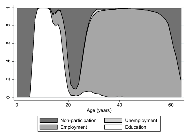
Figure 1: Life-cycle profile for the male cohort born in 1919-21

• Notes: The figure shows the share of individuals in four mutually exclusive states: non-participation, unemployment, employment, and education (including school, vocational training, and further education).

1970 Population and Occupation Census.

The GHS has two limitations for our purposes: the relatively small sample size and the focus on specific birth cohorts. These caveats limit its usefulness in examining how individual war experiences vary across cohorts. Therefore, for this type of analysis, we use a second data set, the West German population and occupation census of May 1970. The data, provided by FDZ der Statistischen Ämter des Bundes und der Länder, (2008), comprise a 10% random sample of the West German population, almost 6,2 million individuals. The census contains information on an individual’s residence on September 1, 1939 (or the father’s residence for individuals born after that date). As in the GHS, we drop migrants from the Soviet occupation zone and define displaced persons as Germans who lived in the eastern territories of the German Reich, Czechoslovakia, or Eastern Europe on September 1, 1939. Unfortunately, we cannot identify war wounded or POWs in the census.

The census provides information only on socioeconomic attainment in 1970 (and thus not across the life cycle). Two outcome variables are nevertheless of interest for our analysis: educational attainment and year of exit from employment. We measure years of education by adding the years spent in vocational training and university to the time required to attain the highest school degree recorded in the data. The census also asked respondents who were not employed in 1970 when they left their last job. For older individuals over the statutory retirement age of 65, we can be reasonably confident that the year indicates the end of their labor market career. Our analysis in Section 4 studies how displacement affected these outcomes for cohorts displaced at different life-cycle stages.

3 Individual Effects of War-Time Shocks over the Life Cycle

We first consider the impact of individual war shocks on labor market outcomes of the 1919-21 cohort. We focus on men and consider three common consequences of war: battlefield injuries, war captivity, and displacement, as defined in Section 2. For each shock, we present two sets of results. First, we report cross-sectional summary measures of labor market success. Second, we show full life-cycle plots for employment and occupational prestige. In addition, we ask whether the observed responses are consistent with the predictions from standard life-cycle models of human capital and labor supply decisions.

Identification.

To identify the effect of distinct shocks, we exploit that battlefield injuries and imprisonment were as good as random, conditional on serving in the war. Enlistment was near-universal for the 1919-21 cohort (Overmans, , 1999), with 95% of men in our sample fighting in the war. Qualified individuals in the arms industry were initially spared from military service (Müller, , 2016), reducing their risk of being injured or imprisoned. However, the 1919-21 cohort was too young to fill positions important to arms production, as the outbreak of WWII coincided with their entry into the labor market. Indeed, men in our data differ hardly in the year of war entry, as the 1919 and 1920 cohorts formed the backbone of Hitler’s Wehrmacht from the beginning of the war.

The cohort was also too young to reach the middle and higher officer ranks, who had been less likely to die in past wars than regular soldiers. Even the lower officer ranks of captains and majors were significantly older than the 1919-21 cohort in 1942, averaging 33.5 and 26.5 years of age, respectively (Förster, , 2009). Moreover, unlike in previous wars, there was a high casualty rate among officers in WWII (Müller, , 2016). Instead, the likelihood of injury and duration of imprisonment depended primarily on which part of the front the soldiers were fighting, over which they had little control. Notably, the soldiers’ region of deployment did not depend on their regions of origin (Overmans, , 1999). And while the very young and old were more likely to be released early (Overmans, , 2000), our analysis conditions on age.

Identification could potentially be more problematic in the case of displacement, as Germans in the former eastern territories may not have been fully comparable to those from other regions. Bauer et al., (2013) show, however, that the differences between displaced and non-displaced West Germans born between 1906 and 1925 were small before the war, not least in education. Importantly, the displaced were not a selected subgroup of their home regions. Virtually all Germans living east of the postwar German-Polish border were displaced. The only major prewar differences between the displaced and the non-displaced were in the proportions employed in agriculture and industry, which can be attributed to the more agrarian structure of prewar East Germany. However, the 1919-21 cohort had little, if any, labor market experience when the war began in 1939, so these structural differences had little impact on their work experience.

We provide evidence in support of these arguments in Appendix Table A3, regressing each shock on prewar characteristics of the respondents (birth year, number of siblings, years of schooling, and an indicator for ill health before or at age 18) and their parents (years of education and the father’s occupational prestige score). Individuals who were sick in childhood were much less likely to serve in the war. Yet, demographic and socio-economic characteristics do not predict war service. Conditional on serving, prewar characteristics also do not predict war injuries, captivity, or displacement, explaining less than 2% of their variation. For robustness, we nevertheless control for birth year indicators, parental education, number of siblings, and time of war entry in our analysis. We show below that our estimates prove insensitive to including these and other controls.

One final concern is that the different shocks could be correlated, such that we capture the consequences of multiple war-related events rather than a clearly defined shock. Yet, displacement is not correlated with either imprisonment or wartime injuries (see Appendix Table C4). We do observe a slight negative correlation between imprisonment and wartime injuries ($\rho=-0.14$), but our results are robust to adding the respective other shocks as controls.

Table 1: The effect of war experiences on labor market outcomes, men born 1919-21

	Educational	Years in employment		Occupational	Old age income from
	attainment	age	age	prestige	work	war victim	non-pension
	(years)	20-55	56-65	(maximum)	pension	pension	sources
	(1)	(2)	(3)	(4)	(5)	(6)	(7)
(a) War injury	-0.263	0.060	-0.908	-0.086	-233.91	180.63	-14.98
(0/1)	(0.199)	(0.320)	(0.290)	(0.987)	(122.80)	(48.76)	(131.74)
	[11.06]	[28.68]	[6.03]	[46.90]	[2390.73]	[20.31]	[375.97]
Observations	465	465	465	465	282	282	297
(b) War captivity	-0.262	-2.266	0.446	-2.879	-11.71	-121.35	-62.98
($>$ 6 months)	(0.224)	(0.332)	(0.332)	(1.201)	(129.94)	(42.21)	(137.43)
	[10.98]	[29.75]	[5.29]	[48.36]	[2301.65]	[146.09]	[377.35]
Observations	331	331	331	296	203	203	216
(c) Displacement	-0.150	-0.638	0.121	-2.424	-80.08	19.74	-310.05
(0/1)	(0.233)	(0.367)	(0.314)	(1.015)	(144.09)	(41.30)	(94.47)
	[10.93]	[28.82]	[5.69]	[47.04]	[2376.11]	[59.57]	[459.16]
Observations	427	427	427	427	254	254	269

• Notes: Regression estimates of the effect of battlefield and other war-related injuries (panel (a)), war captivity (panel (b)), and displacement (panel (c)) on various outcome variables (shown in the table header). Each estimate is from a separate regression. The sample consists of males born 1919-21. Columns (5) to (7) restrict the sample to the second part of GHS-2 conducted in 1987/88 where we observe individuals up to age 65-69 (see Footnote 5). All regressions control for the birth year (indicators), years of schooling of father and mother, number of siblings, and time of entry into the war. Robust standard errors are shown in parentheses, unconditional means for the unaffected control group are in square brackets.

Battlefield and other war-related injuries.

Panel (a) of Table 1 summarizes how battlefield injuries affected individuals’ labor market careers. Two main findings emerge. First, men with battlefield injuries were less likely to be employed at older ages than their non-injured peers, although they achieved similar levels of employment in their earlier working years (see columns (2) and (3)). War injuries reduced employment by nearly one year between ages 56-65, as they accelerated the transition from work to retirement. Second, war injuries reduced monthly work pensions by about DM 234 or almost 10% compared to the control mean (column (5)). However, the higher pension payments as war victims almost compensated for this loss (column (6)). These results are robust to alternative control variables (see Appendix Table C5).

The detailed life-cycle graph in panel (a) of Figure 2 confirms that the adverse effect of war injuries on employment arose only late in life. Employment probabilities of men with and without injuries were similar until age 50 but started diverging in the early 50s. The gap then widened steadily until age 61, reaching 17 percentage points, before shrinking again as injured and non-injured veterans retired. On average, the employment probability of injured veterans was 8.5 percentage points lower between ages 56 and 65 than that of non-injured peers (relative to a baseline probability of 60.9%). Perhaps surprisingly, we do not find an effect of wartime injuries on occupational success (see panel (b) of Figure 2).

Figure 2: Life-cycle effects of war experiences, men born 1919-21

War injury

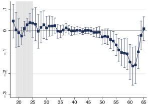
(a) Employment

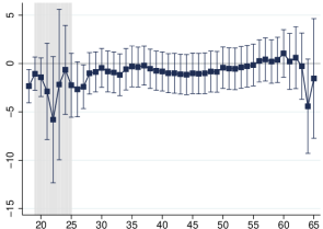
(b) Occupational Prestige

War captivity

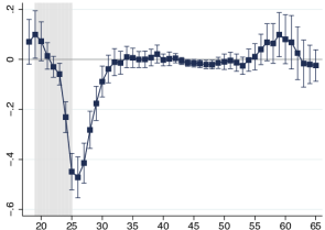
(c) Employment

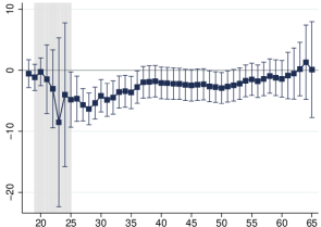
(d) Occupational prestige

Displacement

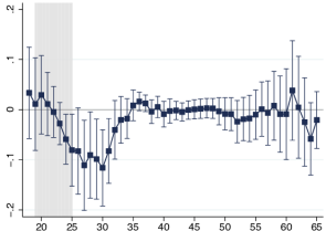
(e) Employment

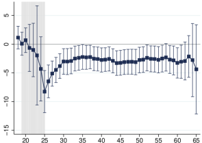
(f) Occupational prestige

• Notes: Estimated effect of battlefield and other war-related injuries (panels (a) and (b)), war captivity (panels (c) and (d)), and displacement (panels (e) and (f)) on employment (panels on the left) and occupational prestige (conditional on employment, panels on the right) over the life cycle. Estimates are from a pooled OLS regression, interacting the regressor of interest and birth year (indicators) with a full set of age indicators. The sample consists of males born 1919-21. Point estimates are marked by a dot. The vertical bands indicate the 95% confidence interval of each estimate. The shaded area indicates the duration of WWII.

As detailed in Appendix D, the life-cycle patterns of injured veterans’ employment documented here are in line with a standard Ben-Porath type of model with endogenous retirement decisions (Hazan, , 2009). We assume that war injuries such as bullet wounds or amputations increase the disutility of work, which tends to decrease employment. But, as the disutility of work also increases in age, an upward shift in this disutility does not affect employment in early or mid-career; instead, the war injured are predicted to advance their entry into retirement, as observed in our setting. By mitigating the income loss from early retirement, the provision of pensions for war victims increases the incentives for early retirement further. Our findings are, therefore, in line with basic economic mechanisms and might extend to other settings: for example, we would expect the effects of the recent Russo-Ukrainian war on veterans’ labor supply to be strongest not in the immediate post-war period, but in 20-30 years, when those veterans approach retirement age.

Prisoners of war.

We next consider the effect of being taken POW for more than six months, a fate shared by nearly half of the men in our data. POWs born in 1919-21 were in captivity at a time when–in peacetime–they would have completed their education and entered the labor market. Panel (b) of Table 1 shows that they received slightly less education as a result (column (1)) and were employed for about 2.3 fewer years between ages 20 and 55 (column (2)). They also had less occupational success than veterans who escaped war captivity (column (4)). Nevertheless, POWs did not receive much lower work pensions (column (5)), as Germany’s pension system “replaces” gaps in the employment biography caused by war captivity (see Appendix B.2).

Panel (c) of Figure 2 illustrates how war captivity delayed labor market entrance. POWs were significantly less likely to be employed in their 20s, with the gap peaking at nearly 50 percentage points in their mid-20s. However, POWs managed to close the employment gap in their 30s and were more likely to work in later life. POWs’ probability of employment overtook that of non-POWs at age 55. The gap widens until age 59, when POWs were 9.9 percentage points more likely to be employed than non-POWs, before closing again. POWs experienced lower occupational success than non-POWs throughout their careers, although the gap gradually closes over time (panel (d)).

As shown in Appendix D, the effects of imprisonment on educational attainment and retirement decisions are again in line with the predictions from standard life-cycle theory. By reducing the potential duration of an individual’s productive working span, imprisonment discourages educational attainment. Moreover, by reducing labor earnings, war captivity increases the marginal utility of consumption and, therefore, participation–POWs postpone their retirement entry to compensate for the lost working time during captivity.

Displacement.

More than one in five men in our sample was forcibly displaced from Eastern Europe. Panel (c) of Table 1 shows that between the ages of 20 and 55, displaced persons were employed for about 0.6 years less than their non-displaced peers (column (2)), but their employment at older ages was similar (column (3)). Consistent with its negative impact on employment, displacement reduced the maximum occupational prestige attained over a lifetime by 2.4 points (or 5% relative to the mean prestige score of the control group). The displaced also had a significantly lower income in old age than the non-displaced, mainly due to differences in non-retirement income such as rental income, interest, or dividends: displacement lowered income from non-pension sources by DM 310 per month or almost 68% relative to the control mean (Column (7)).

Panels (e) and (f) of Figure 2 show that displacement left clear traces in labor market careers. The first key result is that immediately after the war, displaced persons were up to 10 percentage points less likely to be employed than non-displaced persons (panel (e)). The employment gap began to close when the displaced were in their early 30s and disappeared when they were in their mid-30s. The second key result is that the occupational prestige of displaced persons remained significantly lower throughout their labor market careers. Panel (f) illustrates that the loss of occupational prestige was greatest at about age 25, shortly after displacement. While this penalty declined in the late 20s, it remained unchanged or even increased slightly thereafter. At age 56-65, displacement still lowered occupational prestige by around 3.4 points (or 7.8% relative to the control mean).

In Appendix D, we interpret displacement as a decline in the wage rate (e.g., due to a loss of social networks or region-specific human capital) or a loss of wealth (e.g., due to the loss of property). A wage decline generates opposing income and substitution effects and, therefore, ambiguous implications for the retirement decision. In a simple model with log-linear utility, the income and substitution effects cancel out exactly. On the other hand, a pure wealth effect would generate an income but no substitution effect and therefore delay retirement. These implications align with the observation that expellees do not retire (significantly) later. However, as we show next, the effects of displacement depend critically on the age at which a person was displaced, with strong effects on education and employment for some age groups.

4 The Effect of Displacement across Cohorts

This section studies how the impact of displacement on educational attainment and employment varies across cohorts. Our analysis draws mostly on the 1970 census, which has a sufficiently large sample size to identify the consequences of displacement by cohort. Figure 3 summarizes our findings.

Figure 3: The impact of displacement on education and employment

(a) Average years of education

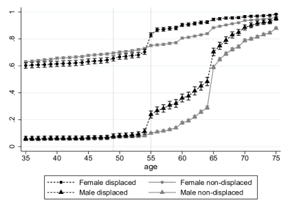
(b) Employment exit by age, 1890 cohort

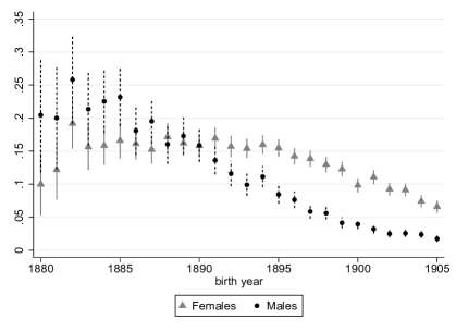
(c) Immediate effect on employment exit

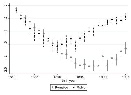
(d) Total employment effect (years)

• Notes: The figure illustrates the impact of displacement on education and employment across cohorts. Panel (a) shows unconditional means in years of education by cohort and displacement status. Panel (b) depicts for one particular cohort, born in 1890, the probability of having exited employment for displaced and non-displaced persons over the life-cycle. Gray vertical lines indicate the beginning and end of WWII. Panel (c) estimates the immediate effects of displacement on the probability to exit from employment for cohorts born between 1880 and 1905. Effect estimates are from DiD regressions, with displaced persons as the treatment group and 1938 as the pre- and 1946 as the post-treatment period. Panel (d) estimates the overall impact of displacement on years of employment up to age 65. The effect estimates are from DiD regressions, with displaced workers as the treatment group and 1938 as the pre-treatment period. The post-treatment period extends from 1946 to the year a cohort turns 65. We measure total impacts as the product of the DiD coefficient and the potential years of employment from 1946 to the year a cohort turns 65. Point estimates are indicated by a dot, vertical bands indicate 95% confidence intervals (based on standard errors clustered at the individual level).

Educational attainment.

Panel (a) of Figure 3 compares, separately for men and women, the average educational attainment of displaced and non-displaced persons for cohorts born between 1905 and 1943. We do not include more recent cohorts as they may not have completed their education by 1970.

Among men, we observe nearly identical trends in education for displaced and non-displaced persons born in 1918 or earlier. Beginning with cohorts born around 1920, the average educational attainment of the displaced declined, while it stagnated for the non-displaced. Displacement, therefore, had a slightly negative effect on the education of men who were in their mid-20s at the time of expulsion (consistent with our findings for the 1919-21 cohort in Table 1). This educational penalty gradually increased in subsequent cohorts, reaching a maximum of about 0.7 years for men born around 1930. These are precisely the cohorts that suffered from the turmoil of flight and expulsion during the transition from school to vocational training.

The gap between displaced and non-displaced males shrinks for younger cohorts and turns positive for cohorts who entered school after displacement. Such positive effects could result from the loss of land, which led the children of displaced persons to seek work outside of agriculture, thereby increasing the importance of educational investment (Bauer et al., , 2013). Moreover, the experience of losing property might have encouraged displaced people to invest in “portable assets” such as education (Brenner and Kiefer, , 1981; Becker et al., 2020a, ).

Similar patterns emerge for women: Displaced women born around 1930 suffered high educational losses of about 0.4 years, while women displaced at young age had higher educational attainment than their non-displaced counterparts. The gap between the displaced and the non-displaced opens later for women than men, around the 1926/27 cohort, perhaps because women in earlier cohorts were more likely to have completed their education when the war began (as they had, on average, lower education than men). Moreover, women’s educational careers were less directly interrupted by the war, while the military draft forced men to postpone further educational investments.

One drawback of the 1970 census data is that we cannot observe parental education. However, we observe similar patterns in the GHS in regressions that condition on parental covariates (see Appendix Table C6). We also verify in the GHS that the educational gap between displaced and non-displaced in the 1929-31 cohort opens only with displacement (see Appendix Figure C3).

Employment.

Displacement had little impact on the retirement behavior of men who experienced WWII as young adults (Section 3), but how did it affect women or older cohorts? We use information on an individual’s last employment to define an indicator variable that takes the value of one for years in which an individual has left gainful employment (“employment exit”). Panel (b) of Figure 3 illustrates how the probability of exiting employment evolves over the life cycle, distinguishing between displaced and non-displaced persons. The plot focuses on one particular cohort born in 1890 (Appendix Figure C4 shows similar plots for cohorts born in 1885, 1895, and 1900). We observe a pronounced spike in employment exits for displaced persons in 1945 when most displacements occurred (the second gray vertical line in the figure indicates the corresponding age of 55). In contrast, there is no similar spike for the non-displaced, for whom the exit probability evolves smoothly around 1945. The employment gap between the groups, therefore, widened sharply at the time of displacement.

Importantly, this effect of displacement on employment varies greatly by birth cohort and gender. Panel (c) of Figure 3 illustrates this pattern in detail, reporting the immediate employment effect of displacement for each cohort born between 1880 and 1905. Estimates are from simple Difference-in-Differences (DiD) regressions, with 1938 as the pre- and 1946 as the post-treatment period. These regressions measure the difference between displaced and non-displaced individuals in the change in the labor market exit probability between 1938 and 1946.

Panel (c) shows that for men born in 1885, displacement increased the probability of employment exit in 1946 by 23.2 percentage points (relative to a post-treatment control mean of 19.3). The effect gradually declines for younger cohorts, to less than 1.7 percentage points for men born in 1905. The immediate effects of displacement on employment are more stable with age for women. For older women born in 1885, displacement increased the probability of exiting the labor market by 16.6 percentage points in 1946. The effect size is substantial, given that only a third had not yet left the labor market by 1938. Thus, half of the women still “at risk” of exiting did so due to displacement. Displacement also had a much greater effect on younger women than on men: Among women born in 1905, 6.9 percentage points left employment permanently by 1946 as a result of displacement. We suspect that the displacement effect is larger for women than men because the former were generally less attached to the labor market.

While the immediate impact is smaller for younger cohorts, especially for men, the young have a longer labor market career ahead of them. An earlier exit from the labor force is, therefore, more consequential for their careers. Panel (d) of Figure 3 depicts the total effect of displacement on years of employment up to age 65, the statutory retirement age. We quantify the total employment effect as the cumulative difference in employment from 1946 to the year a cohort turns 65. For men, the total employment effect of displacement follows a hump shape: Older cohorts lost little time in employment because they were close to retirement anyway. The employment loss then gradually increases with birth year, peaking at about 1.5 years for men born in 1890-95. Younger male cohorts again lost very little employment time, as only a few exited employment after displacement. For women, on the other hand, the overall employment loss is largest for the relatively young cohorts born in 1895-1905. They lost more than two years of employment due to displacement.

In Appendix D, we show that the observed variation in the employment effect is consistent with simple theoretical arguments. A reduction in the wage rate due to displacement generates a negative substitution effect (as work is being less rewarded) and a positive income effect (as life-cycle earnings and consumption decrease). However, this income effect depends on the age at which an individual is being displaced. Individuals close to their expected retirement age experience only a minor income effect, as most of their life-cycle earnings have already been realized–their employment response is dominated by the substitution effect, and hence negative. In contrast, younger individuals experience a more sizable income effect due to displacement, muting the response in employment.

5 Conclusion

The dramatic return of war and displacement to Europe following Russia’s attack on Ukraine has reignited interest in the labor market consequences of violent conflict. Our study examines the impact of battlefield injuries, war captivity, and displacement in the context of WWII, the most devastating conflict in history. We show that the economic consequences of these shocks often became visible long after the war. For example, the effect of war injuries on the employment of veterans was most pronounced not in the immediate postwar period, but decades later, as these veterans approached retirement. Displacement also had very different effects depending on the age and gender of the displaced. The impact on education was worst for students facing the critical transition from school to vocational training. On the other hand, the loss in employment was particularly severe for women and older male cohorts. Overall, our findings suggest that policies to alleviate the hardships of war should take into account that its consequences depend critically on age-at-exposure and vary greatly over the life cycle.

Online Appendix

Appendix A Data Appendix

A.1 Educational attainment

The GHS indicates the highest school-leaving and vocational training qualifications that a person has obtained (if any). Using this information, we calculate years of schooling as the minimum duration required to earn a particular degree. To determine the total number of years of education, we add to the years of schooling the minimum length of time required to earn a particular vocational education degree. Table A1 shows the minimum length of time we use to calculate our measures of education (taken primarily from Müller, , 1979).

Table A1: Minimum lengths of time required to earn a given degree

Degree	Minimum time length
School Degree
No completed school degree	8 years
Sonderschulabschluss (special needs school)	8 years
Volks-/Hauptschulabschluss (low school track)	8 years
Mittlere Reife (medium school track)	10 years
Fachhochschulreife (high school track)	12 years
Abitur (high school track)	13 years
Vocational Training Degree
No vocational degree	0 years
Agricultural or household apprenticeship	2 years
Industrial apprenticeship	2 years
Vocational school degree	2 years
Commercial apprenticeship	3 years
Master craftsman	4 years
University of applied sciences degree	4 years
University degree	5 years
Other vocational training degree	2 years

A.2 Individual war shocks

Table A2: Exposure to individual war shocks

	War injuries			War captivity				Displacement
	1919-21 (men)			1919-21 (men)				1919-21	1929-31	1939-41
		Bullet			$>$6	Length
	Share	wounds		Share	months	(months)		Share	Share	Share
	(1)	(2)		(3)	(4)	(5)		(6)	(7)	(8)
Mean	0.299	0.206		0.755	0.474	16.547		0.227	0.182	0.187
Std. dev.	(0.458)	(0.405)		(0.431)	(0.500)	(20.256)		(0.419)	(0.386)	(0.390)

• Notes: Averages and standard deviations (in parenthesis). Statistics for battlefield injuries and war captivity are based on 559 males born 1919-21. War injuries include amputation, frostbite, bullet wound, others. Statistics for displacement are for men and women and based on 1,278 (1919-21 cohort), 661 (1929-31) and 673 (1939-41) observations, respectively (after excluding GDR refugees). The displaced are defined as those individuals who on 1 September 1939 lived in the Eastern territories of the German Reich, Czechoslovakia, or Eastern Europe.

Table A3: Exogeneity of war service and war shocks

	War service	War injuries	War captivity	Displacement
	(1)	(2)	(3)	(4)
Father’s years of schooling	0.003	-0.002	0.004	-0.005
	(0.004)	(0.016)	(0.014)	(0.009)
Mother’s years of schooling	-0.021	-0.02	0.011	0.008
	(0.021)	(0.034)	(0.025)	(0.017)
Father’s occupational score	-0.002	0.003	-0.004	0.000
	(0.001)	(0.002)	(0.002)	(0.001)
Birth year	0.017	-0.026	0.018	0.005
	(0.013)	(0.029)	(0.025)	(0.016)
# siblings	-0.003	0.005	0.011	0.004
	(0.004)	(0.010)	(0.008)	(0.005)
Years of schooling	0.009	-0.028	0.020	0.018
	(0.007)	(0.017)	(0.015)	(0.012)
Poor health at age$\leq$18	-0.454	-0.184	-0.016	-0.110
	(0.168)	(0.142)	(0.214)	(0.086)
Female	–	–	–	0.001
				(0.026)
R2	0.077	0.015	0.012	0.005
N	492	465	465	1,054

• Notes: The table reports coefficient estimates from the indicated war-related shock on a set of individual and parental characteristics for birth cohorts 1919-21. Estimates for war service, injuries and captivity are for men only. Estimates for war injuries and captivity are conditional on war service. Robust standard errors in parentheses.

Appendix B Pension benefits and war compensation

B.1 Compensation programs

Policymakers developed two critical programs to compensate the war-disabled and facilitate their integration into the labor market (Wiegand, , 1995). First, the war victims’ provision (Kriegsopferversorgung) provided compensation and assistance to war-disabled persons, widows, and orphans. The war victims’ pension (Kriegsopferrente) was paid to persons who suffered severe health damage due to military service; see Section B.2 for details.

Second, the 1952 Equalization of Burdens Act partially compensated for the loss of wartime property, distributing wartime burdens more evenly throughout society. Those whose property had been spared by the war were to compensate those who had suffered war damage. Under the same law, displaced persons could also apply for grants to start businesses and public assistance in finding housing. However, the Equalization of Burdens Act had only limited success in restoring the occupational status of the displaced and the wealth distribution that had existed before the war (Falck et al., , 2012; Wiegand, , 1995).

B.2 Pension benefits and World War II

Statutory pensions in Germany depend on the labor income earned over the life course. The longer people work and the more they earn, the higher their pensions. The German pension system thus “insures” living standards achieved during working life and extends prosperity into retirement. Since the pension reform of 1957, the system has been organized as a pay-as-you-go-scheme. This means that current contributions (from employees and employers) pay for current pension obligations. The 1957 reform also made pensions dynamic by linking them to wage trends. Entitlement to a pension arises when individuals have paid contributions for at least five years. Before 1992, the retirement age was 65 for men and 60 for women. Early retirement was possible under certain conditions for the disabled and long-term unemployed.

Importantly, the pension system smooths out gaps in the employment biography caused by compulsory state measures such as military service, war captivity, expulsion, and resettlement. These “substitute periods” (Ersatzzeiten) are fully taken into account when calculating the pension. In addition, “periods of absence” (Ausfallzeiten) are taken into account in the pension calculation. Periods of absence are periods during which employment is interrupted for personal reasons, including unemployment, incapacity to work, pregnancy, and further education.

The pension system also covers the financial loss caused by the death of a spouse. The survivor’s pension (Witwenrente) is intended to replace the support previously provided by the deceased. Until 1986, women received survivor’s pension unconditionally and regardless of their own work history. Widowers, on the other hand, were entitled to a survivor’s pension only if the deceased’s wife had provided most of the family’s support. This differential treatment did not end until 1986.

War victims receive additional pension benefits. The war victim’s pension (Kriegsopferrente) is paid to persons who have suffered serious health damage as a result of military or military-like service in connection with the war (e.g. damages due to direct warfare, captivity, or internment abroad). The basic income support (Grundrente), which is paid as part of the war victim’s pension, is not means-tested. Instead, its amount depends only on the severity of the health damage caused by the war. Severely disabled persons who can no longer work receive an additional means-tested compensatory pension (Ausgleichsrente). If an injured person dies as a result of his injury, his widow receives survivor’s pension.

Appendix C Additional Figures and Tables

C.1 Figures

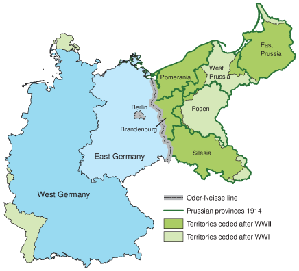
Figure C1 : German territorial losses in World War I and II

• Base maps: MPIDR and CGG, (2011).

Figure C2 : Education, participation, and non-participation over the life cycle, by gender and cohort

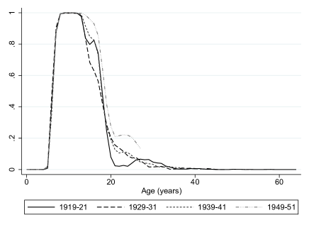
(a) Men, education

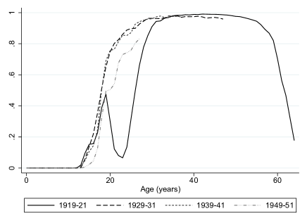
(b) Men, participation

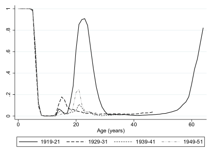
(c) Men, non-participation

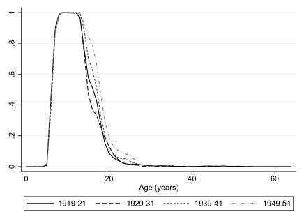
(d) Women, education

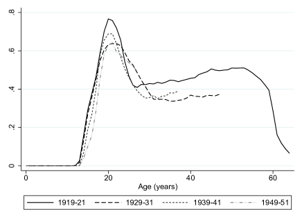
(e) Women, participation

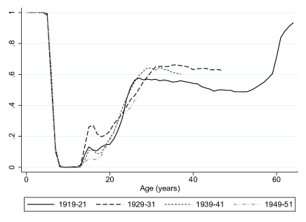
(f) Women, non-participation

• Notes: The graph depicts, separately by gender, the share of individuals in education (Panels (a) and (d)), in the labor force (Panels (b) and (e)) and non-participating (Panels (c) and (e)). We distinguish between cohorts born in 1929-21, 1929-31, 1939-41 and 1949-51. Education includes schooling, vocational training, and further education. Individuals are in non-participation if they are not in education, do not work, and are not unemployed.

Figure C3 : The effect of displacement on education over the life cycle, cohort born 1929-31

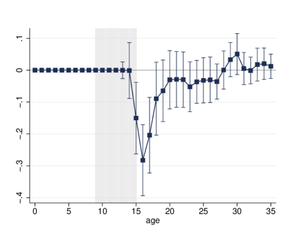
(a) Males

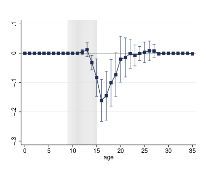
(b) Females

• Notes: The graph depicts estimated differences in educational participation between displaced and non-displaced individuals over the life cycle, drawing on GHS data. Estimates come from conditional OLS regressions, controlling for the father’s and mother’s years of schooling and number of siblings. Point estimates are marked by a dot. The vertical bands indicate the 95% confidence interval of each estimate. The shaded area indicates the duration of WWII.

Figure C4 : Employment exit probability over the life cycle, by cohort

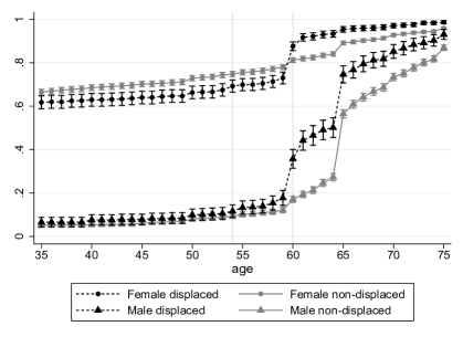
(a) 1885

(b) 1890

(c) 1895

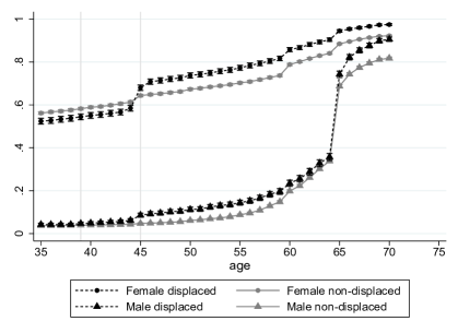
(d) 1900

• Notes: The figures depict, by cohort, the probability of having exited employment for displaced and non-displaced persons over the life cycle. Gray vertical lines indicate the beginning and end of WWII. Vertical bands indicate 95% confidence interval.

C.2 Tables

Table C4: Correlation between war-related shocks

	War injuries	War captivity	Displacement
	(1)	(2)	(3)
War injuries	1.000	–	–
War captivity	-0.107	1.000	–
Displacement	0.041	0.014	1.000

• Notes: Correlations between individual war shocks, men born in 1919-21 (N=529).

Table C5: Robustness tests on the effect of different war-related shocks, men born 1919-21

	Educational	Years in employment		Occup.	Old age income from
	attainment	age	age	prestige	work	war victim	non-pension
	(years)	20-55	56-65	(maximum)	pension	pension	sources
	(1)	(2)	(3)	(4)	(5)	(6)	(7)
A. War injury (0/1)
Raw	-0.434	-0.031	-1.008	-0.458	-263.98	195.57	23.89
	(0.204)	(0.307)	(0.272)	(0.957)	(122.75)	(51.58)	(134.43)
Baseline	-0.263	0.060	-0.908	-0.086	-233.91	180.63	-14.98
	(0.199)	(0.320)	(0.290)	(0.987)	(122.80)	(48.76)	(131.74)
Extended	-0.269	-0.073	-0.863	-0.289	-233.03	173.50	-18.30
	(0.204)	(0.315)	(0.291)	(0.992)	(122.98)	(45.03)	(136.79)
B. War captivity ($>$ 6 months)
Raw	-0.413	-2.286	0.386	-3.396	35.07	-131.28	-88.68
	(0.237)	(0.318)	(0.324)	(1.170)	(125.36)	(44.91)	(133.53)
Baseline	-0.262	-2.266	0.446	-2.879	-11.71	-121.35	-62.98
	(0.224)	(0.332)	(0.332)	(1.201)	(129.94)	(42.21)	(137.43)
Extended	-0.273*	-2.293	0.337	-2.797	-5.21	-83.54	-76.34
	(0.165)	(0.377)	(0.339)	(1.158)	(127.83)	(31.67)	(144.28)
C. Displacement (0/1)
Raw	-0.087	-0.854	-0.074	-2.351	-99.85	39.58	-303.93
	(0.233)	(0.356)	(0.286)	(0.990)	(131.29)	(44.81)	(78.99)
Baseline	-0.150	-0.638	0.121	-2.424	-80.08	19.74	-310.05
	(0.233)	(0.367)	(0.314)	(1.015)	(144.09)	(41.30)	(94.47)
Extended	-0.280	-0.603	0.091	-2.769	-98.73	20.83	-326.20
	(0.161)	(0.370)	(0.309)	(0.942)	(136.59)	(41.48)	(95.99)

• Notes: Regression estimates of the effect of war-related shocks on various outcome variables (shown in the table header). Each estimate is from a separate regression. The sample consists of males born 1919-21. Columns (5) to (7) restrict the sample to the second part of GHS-2 conducted in 1987/88 where we observe individuals up to age 65-69 (see Footnote 5). The “raw” specification controls only for birth year (indicators). The “baseline” specification additionally controls for years of schooling of father and mother, number of siblings and time of entry into the war. The “extended” specification additionally controls for own years of schooling (all panels) and imprisonment (panel A) or war injuries (panel B). Robust standard errors are shown in parentheses, unconditional means for the unaffected control group are in square brackets.

Table C6: The effect of displacement on education, by sex and cohort

	Males				Females
	1919-21	1929-31	1939-41		1919-21	1929-31	1939-41
	(1)	(2)	(3)		(4)	(5)	(6)
Displacement (0/1)	-0.150	-0.652	0.074		0.360	-0.825	0.207
	(0.233)	(0.274)	(0.343)		(0.202)	(0.242)	(0.403)
	[10.934]	[10.693]	[10.782]		[9.732]	[9.447]	[9.988]
Observations	427	303	310		605	303	298

• Notes: The table shows, by sex and cohort, estimates of the effect of displacement on years of education, drawing on data from the GHS. Estimates come from conditional OLS regressions. Years of education include time spent in vocational training and at university. All regressions control for birth year (indicators), years of schooling of father and mother, number of siblings and (for males) time of entry into the war. Robust standard errors are shown in parentheses, unconditional means for the non-displaced control group in square brackets.

Appendix D Theoretical Predictions

How do war-related shocks affect an individuals’ education and labor market outcomes over the life course, and can standard theory capture those effects? In this section we derive theoretical predictions from a standard life-cycle model of human capital and retirement decisions.

D.1 A Ben-Porath model with endogenous retirement

Summarizing a version of the Ben-Porath model with endogenous retirement decisions (Hazan, , 2009), assume that an individual’s lifetime utility $V$ equals

$$V=\int_{0}^{T}e^{-\rho t}u(c(t))dt-\int_{0}^{R}e^{-\rho t}f(t)dt,$$ (D-1)

where $c(t)$ is consumption at age $t$, $f(t)$ is the disutility of work (assumed to satisfy $f^{\prime}(t)=0$ and $f(T)=\infty$), $\rho$ is the subjective discount rate, $R$ is the retirement age, and $T$ is the length of the individual’s lifetime.

Human capital $h(s)$ and therefore the wage $w$ depend on the individual’s choice of the length of schooling prior to entering the labor market $s$ and “learning speed” $\theta(s)$, such that $w=h(s)=e^{\theta(s)}$. The sole costs of schooling is foregone earnings, so the budget constraint

$$\int_{s}^{R}e^{-rt}e^{\theta(s)}dt=\int_{0}^{T}e^{-rt}c(t)dt$$ (D-2)

equates consumption over the lifetime (between 0 and $T$) with earnings over the working life (between $s$ and $R$), where $r$ is the interest rate. Following Hazan, (2009), we assume $r=\rho$, implying that consumption is constant over the life cycle,

$$c(s,R)=\frac{e^{\theta(s)}\left(e^{-rs}-e^{-rR}\right)}{1-e^{-rT}}.$$ (D-3)

Solving the Lagrangian associated with maximizing lifetime utility $V$ leads to the two equilibrium conditions equating the marginal costs of schooling with its marginal benefits,

$$\frac{1}{\theta^{\prime}(s)}=\frac{1-e^{-r(R-s)}}{r}$$ (D-4)

and the disutility of work at age $R$ with the marginal utility of working (in terms of consumption)

$$f(R)=u^{\prime}(c(s,R))e^{\theta(s)}.$$ (D-5)

Figure D5a provides a numerical example, assuming $u(\cdot)=log(\cdot)$, $f(R)=1/(1-R)$, $T=r=1$ and $\theta(s)=s/0.3$. The (thin) blue line corresponds to the indifference curve associated with the optimal schooling condition in equation (D-4) while the (thick) orange line corresponds to the optimal retirement decision represented by equation (D-5). The optimal schooling and retirement age are determined by the intersection of these two curves (point A).

Figure D5 : Theoretical predictions

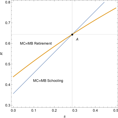
(a) Baseline

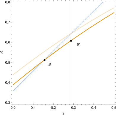
(b) War-related injury

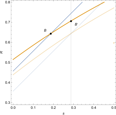
(c) War captivity

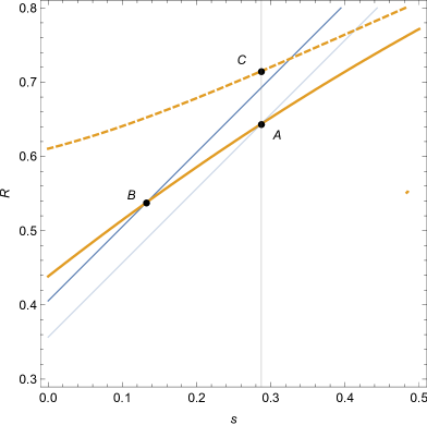
(d) Displacement

• Notes: Numerical illustrations of a Ben-Porath model with retirement decision (Hazan, , 2009). Figure (a) is baseline with $u(\cdot)=log(\cdot)$, $f(R)=1/(1-R)$, $T=r=1$ and $\theta(s)=s/0.3$. Figure (b) corresponds to a war-related injury with an increase in disutility of work such that $f_{injury}(R)=1.2f(R)$. Figure (c) corresponds to war captivity with time $x=0.1$ spent in captivity. Figure (d) corresponds to displacement with a reduction in the wage rate to $\theta_{d}(s)=0.9\theta(s)$ (solid blue and orange lines) or a reduction in wealth such that $c_{d}(s,R)=c(s,R)-1/3$ (dashed orange line).

Using this model, we next derive the implications of different types of war-related shocks–war injuries, captivity, and displacement–for the choice of schooling $s$ and retirement age $R$.

D.2 War injuries

Among men born 1919-21, nearly one third suffered injuries such as bullet and shrapnel wounds, frostbite or amputations (see Table A2). What are the likely implications? Interpreted through the lens of the model, war injuries increase the disutility of work $f(R)$. Moreover, their effect on schooling $s$ will be non-positive, as explained below. The equilibrium condition (D-5) determining the retirement decision then implies that the marginal utility of consumption $u^{\prime}$ must increase, corresponding to a reduction in consumption (and income), and therefore a reduction in the retirement age $R$.

But, war injuries may not only affect the disutility of work, but also generate different types of income effects. First, the war-injured were eligible to a war pension (see Section B.2), corresponding to an increase in income. Second, war-related injuries may reduce productivity, at least in some jobs or for some individuals, corresponding to a decrease in the wage $w=e^{\theta(s)}$ and a decline in income and pensions. The overall effect of war injuries on income is therefore ambiguous. We show in Section 3 that in our setting, the net effect on (labor + war) pensions is negligible. The main channel via which war injuries affect (life-cycle) income is therefore the retirement decision.

The effect of war injuries on schooling $s$ is non-positive. First, note that most of those born in 1919-21 entered the military around age 20, after leaving school. Moreover, military service shortened the remaining lifespan available for work, thereby lowering the incentives for war returnees to invest into education (a positive relation between the length of the economic lifespan and educational investments is a standard implication of the Ben-Porath model; see Ben-Porath, 1967). Indeed, fewer than 10% of returnees entered an apprenticeship after the war. A further shortening of the active working life due to early retirement decreases these incentives further, implying that the effect of war injuries on educational investments are negative.

Figure D5(b) provides a numerical example. The increase in the disutility of work corresponds to a downward shift of the indifference curve associated with condition (D-5). If the war-injured could freely optimize (ex-ante optimization) they would reduce both retirement entry $R$ and their schooling $s$ (point B). However, most have completed their schooling investments before enlistment to the military (vertical line). As they cannot reduce those educational investments ex-post, their incentives to reduce the retirement age are mitigated (point B’). Standard theory therefore predicts that war injuries decrease the retirement age and reduce educational investments in the right tail of the distribution (i.e., among those who had not yet completed their investments before enlistment).

D.3 War captivity

More than three quarters of men born 1919-21 were in captivity, often for years (see Table A2). This captivity disincentives educational investments. While some war returnees entered apprenticeships or studied at a university, those spending time in captivity returned later and would have made such investments later. But a key implication of the Ben-Porath and similar models is that educational investments are less profitable at later ages, when the remaining productive work span is shorter. Formally, the optimal educational investment of war prisoners is determined by

$$\frac{1}{\theta^{\prime}(s)}=\frac{1-e^{-r(R-x-s)}}{r}$$ (D-6)

where $x$ is the time spent in captivity. An increase in $x$ decreases the right hand of this equation, so for the condition to hold we require a reduction of schooling $s$ or an increase in the retirement age $R$ (or both).

Individuals choose their optimal retirement age according to the condition (D-5). Plausibly, the disutility of work on the left-hand side is not much affected by war captivity. But for a given retirement age $R$ and schooling $s$, the right side of (D-5) increases because life-cycle income–and therefore consumption according to equation (D-3)–declines due to war captivity. Specifically, the optimal consumption is now given by

$$c(s,R)=\frac{e^{\theta(s)}\left(e^{-r(s+x)}-e^{-rR}\right)}{1-e^{-rT}}.$$ (D-7)

Therefore, the marginal utility of consumption increases. To ensure that equality (D-5) holds, we therefore need again that the retirement age $R$ increases and/or that $s$ declines.

Figure D5(c) provides a numerical example. Both the indifference curves associated with condition (D-4) and condition (D-5) shift upward, reflecting a decrease in the marginal benefits of schooling for a given level of $R$ and an increase in the marginal utility of working for a given level of $s$. If individuals could freely optimize they would reduce schooling but do not change their retirement age much (point B). However, many individuals will have already completed their schooling investments before enlistment (vertical line). With education above its ex-post optimum, individuals have an incentive to retire later (point B’). Standard theory therefore predicts that war captivity increases the retirement age but reduces educational investments and, therefore, wages.

D.4 Displacement

More than one fifth of our survey respondents are displaced Germans, mostly from the German Reich’s Eastern territories (see Table A2). The extent to which displacement affects educational and labor market careers will depend on the timing of the expulsion. As most displacements occurred towards the end of WWII, they will have only limited effects on the educational investments of older cohorts, including the 1919-21 cohort. In contrast, younger cohorts experienced direct interruptions of their educational careers. For example, the 1929-31 cohort were only 14-16 years olds when the war ended in 1945. As we show in Section 4, displacement therefore led to a large decline in education among younger cohorts.

Here we focus instead on the labor market effects of displacement. Motivated by the evidence shown in Section 4, we assume that displacement reduces an individual’s wage from $\theta(s)$ to $\theta_{d}(s)$, such that $\theta_{d}(s)<\theta(s)$ $\forall s$. The precise reason for this wage decline is not central for our argument, but it might reflect the loss of social networks, specific human capital or “search capital” as the displaced could not return to their previous jobs. This wage decline affects the marginal utility of working $u^{\prime}(c(s,R))e^{\theta(s)}$ on the right-hand side of equilibrium condition (D-5) via two channels. On the one hand, a reduction in the wage $w=e^{\theta(s)}$ directly reduces the incentives to work (substitution effect). On the other hand, a reduction in earnings also reduces consumption $c(s,R)$, thereby increasing the marginal benefits of consumption $u^{\prime}(c(s,R))$ and incentives to work (income effect). As these income and substitution effects have opposing signs, the overall effect on the optimal retirement age $R$ is ambiguous and depends on the curvature of the utility function. A pure wealth effect on the other hand would generate an income but no substitution effect, and therefore lead to an unequivocal postponement of retirement entry.

Figure D5(d) provides a simple illustration for the case of displacement before labor market entry (such as for the 1919-21 cohort). A proportional decrease in the wage rate $w=e^{\theta(s)}$ due to expulsion would shift the indifference curve associated with condition (D-4) upwards (thin blue line). The curve associated with condition (D-5) however remains unchanged in this particular example: as utility is log linear in consumption we have $u^{\prime}(c(s,R))=1/c(s,R)$, and income and substitution effects of a reduction in the wage rate in early life cancel each other out exactly. Ex-ante, expellees would therefore choose lower schooling and an earlier retirement age (point B). However, if educational investments were made before expulsion (as for the 1919-21 cohort) the optimal retirement age remains unchanged (point A). If expulsions affect wealth rather than wages then the curve associated with condition (D-5) would shift, corresponding to a pure income effect (orange dashed line). Assuming schooling is fixed at $s$, individuals would choose a higher retirement age (point C).

But how would the employment effects of displacement vary with age at displacement $d$? The key insight is that the size of the income effect from a reduction in the wage rate depends on the age at which an individual experiences this change. Individuals who are already close to their expected retirement age experience only a minor income effect, as most of their life-cycle earnings have already been realized. The effect of displacement on the employment of older individuals is therefore dominated by the substitution effect, and hence negative. We can show this explicitly by solving for the consumption profile of displaced individuals. Recall that for given life-cycle earnings, the optimal consumption profile is flat. However, as displacement was unexpected, it shifts an individual’s consumption from $c$ to post-displacement consumption $c_{d}$. Focusing on displacement events that occur before retirement ($d<R$) but after the completion of schooling ($d>s$), the budget constraint of a displaced individual is therefore given by

$$\int_{s}^{d}e^{-rt}e^{\theta(s)}dt+\int_{d}^{R_{d}}e^{-rt}e^{\theta_{d}(s)}dt=\int_{0}^{d}e^{-rt}cdt+\int_{d}^{T}e^{-rt}c_{d}dt$$ (D-8)

where the left-hand side is the sum of present discounted value of earnings at wage $e^{\theta(s)}$ before displacement (between end of schooling $s$ and displacement $d$) and at wage $e^{\theta_{d}(s)}$ after displacement (between $d$ and new retirement age $R_{d}$), and the right side is the PDV of consumption $c$ in the pre- and consumption $c_{d}$ in the post-period. Solving the budget constraint for $c_{d}$ and simplifying, we have

$$c_{d} =\frac{e^{\theta(s)}\left(e^{-rd}-e^{-rs}\right)+e^{\theta_{d}(s)}\left(e^{-rR_{d}}-e^{-rd}\right)-c\left(e^{-rd}-1\right)}{e^{-rT}-e^{-rd}}$$

$$=c+\left(e^{\theta_{d}(s)}-e^{\theta(s)}\right)\frac{e^{-rd}-e^{-rR}}{e^{-rd}-e^{-rT}}+\left(e^{-rR}-e^{-rR_{d}}\right)\frac{e^{\theta(s)}}{e^{-rd}-e^{-rT}}.$$ (D-9)

The difference between consumption after displacement $c_{d}$ and consumption $c$ in the pre-period (which itself is a function of schooling $s$ and the planned retirement age $R$) depends on the difference between the old and new wage rate, weighted by the relative lengths of the post-displacement working ($R-d$) and consumption spells ($T-d$). For example, if displacement occurs at the end of the working life ($d=R$), then the weight equals zero and consumption remains unaffected; the individual experiences only a substitution effect. In contrast, if displacement occurs earlier in the career ($R-d\gg 0$) then the weight will be closer to one, and the decline in consumption can be substantial; the individual experiences an income effect. This reduction in consumption maps into a corresponding increase in the marginal utility, counteracting the substitution effect from a decline in wages. Consumption post-displacement also depends on the gap between the initially planned and new post-displacement retirement ages, $R$ and $R_{d}$; an unplanned early retirement due to displacement might necessitate a sudden and large reduction in consumption.

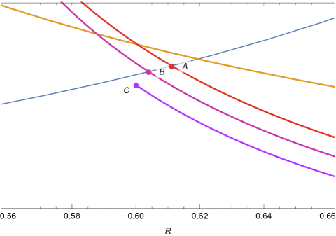
Figure D6 : Theoretical predictions: Displacement by age

• Notes: Numerical illustrations of a Ben-Porath model with retirement decisions (Hazan, , 2009) with $u(\cdot)=log(\cdot)$, $f(R)=1/(1-R)$, $T=r=1$, $\theta(s)=4s$ and $\theta_{d}(s)=3s$. The thin blue line corresponds to the the disutility of work $f(R)$. The orange line corresponds to the marginal utility of working $u^{\prime}(c(s,R))e^{\theta(s)}$. The red, red-purple and purple lines correspond to the marginal utility of working if an individual is displaced at age $d=0.5,d=0.55$ or $d=0.6$.

Figure D6 illustrates these arguments by plotting the two sides of the equilibrium condition (D-5) for the optimal retirement decision, over retirement age $R$. The marginal disutility of work $f(R)$ increases (thin blue line) while the marginal benefits $u^{\prime}(c(s,R))e^{\theta(s)}$ decreases over $R$ (orange line). The optimal retirement age corresponds to the intersection of the two curves. The effects of displacement depend on the age at displacement $d$. We compare displacement around mid-age ($d=0.5$) or closer to retirement age ($d=0.6$). For the mid-age worker, the marginal benefits of working change (red line), but they remain greater than the marginal disutility of work at the time of displacement. This individual would therefore not retire immediately, but retire earlier than originally planned (at point A). Intuitively, mid-aged expellees cannot ”afford” to leave the labor force immediately, as their cumulative life-cycle earnings are still low. They retire earlier, but not much earlier than planned. For a worker displaced at older age ($d=0.6$), this income effect is less pronounced, and their response to displacement is instead dominated by the substitution effect. Indeed, in our example the marginal benefit of working (purple line) falls below the marginal disutility of work; the individual would therefore retire immediately after displacement (point C). Point B represents an intermediate case, in which displacement occurs at $d=0.55$. Overall, a simple life-cycle model implies that the immediate effect of displacement on employment exit increases with age-at-displacement, in line with the empirical pattern shown in Figure 3 (panel (c)).

A similar mechanism could explain why the displacement effect increases less steeply with age-at-displacement for women than men. At the time of our study, most women were married and rarely the main breadwinner in the household. The marginal benefits of working will therefore tend to be lower but also flatter over retirement age $R$ for women (as consumption is less dependent on own than on the spouse’s employment). This has two implications. First, young women may leave the labor force in response to displacement, while this is unlikely to be the case for young men. Second, the employment effects of displacement are reduced for older women, as many will have left the labor force already.

References

- Akbulut-Yuksel, (2014) Akbulut-Yuksel, M. (2014). Children of war: The long-run effects of large-scale physical destruction and warfare on children. The Journal of Human Resources, 49(3):634–662.
- Akbulut-Yuksel et al., (2022) Akbulut-Yuksel, M., Tekin, E., and Turan, B. (2022). World War II blues: The long-lasting mental health effect of childhood trauma. Working Paper 30284, National Bureau of Economic Research.
- Angrist and Krueger, (1994) Angrist, J. and Krueger, A. B. (1994). Why do World War II veterans earn more than nonveterans? Journal of Labor Economics, 12(1):74–97.
- Bauer et al., (2013) Bauer, T. K., Braun, S., and Kvasnicka, M. (2013). The economic integration of forced migrants: Evidence for post-war Germany. The Economic Journal, 123(571):998–1024.
- (5) Becker, S. O., Grosfeld, I., Grosjean, P., Voigtländer, N., and Zhuravskaya, E. (2020a). Forced migration and human capital: Evidence from post-WWII population transfers. American Economic Review, 110(5):1430–63.
- (6) Becker, S. O., Mergele, L., and Woessmann, L. (2020b). The separation and reunification of Germany: Rethinking a natural experiment interpretation of the enduring effects of Communism. Journal of Economic Perspectives, 34(2):143–71.
- Ben-Porath, (1967) Ben-Porath, Y. (1967). The production of human capital and the life cycle of earnings. Journal of Political Economy, 75(4):352–352.
- Bleakley, (2010) Bleakley, H. (2010). Health, human capital, and development. Annual Review of Economics, 2(1):283–310.
- Bound and Turner, (2002) Bound, J. and Turner, S. (2002). Going to war and going to college: Did World War II and the G.I. Bill increase educational attainment for returning veterans? Journal of Labor Economics, 20(4):784–815.
- Brenner and Kiefer, (1981) Brenner, R. and Kiefer, N. M. (1981). The economics of the diaspora: Discrimination and occupational structure. Economic Development and Cultural Change, 29(3):517–534.
- Brückner and Mayer, (1987) Brückner, E. and Mayer, K. U. (1987). Lebensgeschichte und Austritt aus der Erwerbstätigkeit im Alter – am Beispiel der Geburtsjahrgänge 1919-21. Zeitschrift für Sozialisationsforschung und Erziehungssoziologie, 7(2):101–116.
- Cervellati and Sunde, (2013) Cervellati, M. and Sunde, U. (2013). Life expectancy, schooling, and lifetime labor supply: Theory and evidence revisited. Econometrica, 81(5):2055–2086.
- Costa, (2012) Costa, D. L. (2012). Scarring and mortality selection among Civil War POWs: A long-term mortality, morbidity, and socioeconomic follow-up. Demography, 49(4):1185–1206.
- Costa et al., (2020) Costa, D. L., Yetter, N., and DeSomer, H. (2020). Wartime health shocks and the postwar socioeconomic status and mortality of Union Army veterans and their children. Journal of Health Economics, 70:102281.
- Cousley et al., (2017) Cousley, A., Siminski, P., and Ville, S. (2017). The effects of World War II military service: Evidence from Australia. The Journal of Economic History, 77(3):838–865.
- FDZ der Statistischen Ämter des Bundes und der Länder, (2008) FDZ der Statistischen Ämter des Bundes und der Länder (2008). Volkszählung 1970. Scientific-Use-File, own calculations.
- Förster, (2009) Förster, J. (2009). Die Wehrmacht im NS-Staat. Eine strukturgeschichtliche Analyse. Oldenbourg Wissenschaftsverlag, Munich.
- Fortson, (2011) Fortson, J. G. (2011). Mortality risk and human capital investment: The impact of HIV/AIDS in Sub-Saharan Africa. The Review of Economics and Statistics, 93(1):1–15.
- Hazan, (2009) Hazan, M. (2009). Longevity and lifetime labor supply: Evidence and implications. Econometrica, 77(6):1829–1863.
- Heckman, (1976) Heckman, J. J. (1976). A life-cycle model of earnings, learning, and consumption. Journal of Political Economy, 84(4, Part 2):S9–S44.
- Ichino and Winter-Ebmer, (2004) Ichino, A. and Winter-Ebmer, R. (2004). The long-run educational cost of World War II. Journal of Labor Economics, 22(1):57–87.
- Jürges, (2013) Jürges, H. (2013). Collateral damage: The German food crisis, educational attainment and labor market outcomes of German post-war cohorts. Journal of Health Economics, 32(1):286–303.
- Kesternich et al., (2020) Kesternich, I., Siflinger, B., Smith, J. P., and Steckenleiter, C. (2020). Unbalanced sex ratios in Germany caused by World War II and their effect on fertility: A life cycle perspective. European Economic Review, 130:103581.
- Kesternich et al., (2014) Kesternich, I., Siflinger, B., Smith, J. P., and Winter, J. K. (2014). The effects of World War II on economic and health outcomes across Europe. The Review of Economics and Statistics, 96(1):103–118.
- Kesternich et al., (2015) Kesternich, I., Siflinger, B., Smith, J. P., and Winter, J. K. (2015). Individual behaviour as a pathway vetween early-life shocks and adult health: Evidence from hunger episodes in post-war Germany. The Economic Journal, 125(588):F372–F393.
- Kroener et al., (1988) Kroener, B. R., Müller, R.-D., and Umbreit, H. (1988). Organisation und Mobilisierung des deutschen Machtbereichs – Teilband 1: Kriegsverwaltung, Wirtschaft und personelle Ressourcen 1939 bis 1941. DVA Dt. Verlags-Anstalt.
- Kroener et al., (1999) Kroener, B. R., Müller, R.-D., and Umbreit, H. (1999). Organisation und Mobilisierung des deutschen Machtbereichs – Teilband 2: Kriegsverwaltung, Wirtschaft und personelle Ressourcen 1942 bis 1944/45. DVA Dt. Verlags-Anstalt.
- Lee, (2005) Lee, C. (2005). Wealth accumulation and the health of Union Army veterans, 1860–1870. The Journal of Economic History, 65(2):352–385.
- Maas and Settersten, (1999) Maas, I. and Settersten, R. A. (1999). Military service during wartime: Effects on men’s occupational trajectories and later economic well-being. European Sociological Review, 15(2):213–232.
- Manuelli and Yurdagul, (2021) Manuelli, R. E. and Yurdagul, E. (2021). Aids, human capital and development. Review of Economic Dynamics, 42:178–193.
- Mayer, (1995) Mayer, K. U. (1995). Lebensverläufe und gesellschaftlicher Wandel: Die Zwischenkriegskohorte im Übergang zum Ruhestand (Lebensverlaufsstudie LV-West II T - Telefonische Befragung). GESIS Datenarchiv, Köln. ZA2647 Datenfile Version 1.0.0, https://doi.org/10.4232/1.2647.
- Mayer, (2007) Mayer, K. U. (2007). Handbook of Longitudinal Research: Design, Measurement, and Analysis, chapter Retrospective longitudinal research: The German life history study, pages 85–106. Elsevier, San Diego.
- (33) Mayer, K. U. (2018a). Lebensverläufe und gesellschaftlicher Wandel: Die Zwischenkriegskohorte im Übergang zum Ruhestand (Lebensverlaufsstudie LV-West II A - Persönliche Befragung). GESIS Datenarchiv, Köln. ZA2646 Datenfile Version 1.1.0, https://doi.org/10.4232/1.13194.
- (34) Mayer, K. U. (2018b). Lebensverläufe und gesellschaftlicher Wandel: Lebensverläufe und Wohlfahrtsentwicklung (Lebensverlaufsstudie LV-West I). GESIS Datenarchiv, Köln. ZA2645 Datenfile Version 1.1.0, https://doi.org/10.4232/1.13193.
- Mincer, (1997) Mincer, J. (1997). The production of human capital and the life cycle of earnings: Variations on a theme. Journal of Labor Economics, 15(1):26–47.
- Mink et al., (2020) Mink, J., Boutron-Ruault, M.-C., Charles, M.-A., Allais, O., and Fagherazzi, G. (2020). Associations between early-life food deprivation during World War II and risk of hypertension and type 2 diabetes at adulthood. Scientific Reports, 10(1).
- Müller, (2016) Müller, R.-D. (2016). Hitler’s Wehrmacht, 1935–1945. University Press of Kentucky.
- Overmans, (1999) Overmans, R. (1999). Deutsche militärische Verluste im Zweiten Weltkrieg. R. Oldenbourg, Munich.
- Overmans, (2000) Overmans, R. (2000). Soldaten hinter Stacheldraht – Deutsche Kriegsgefangene des Zweiten Weltkriegs. Propyläen, Berlin.
- Ramirez and Haas, (2021) Ramirez, D. and Haas, S. A. (2021). The long arm of conflict: How timing shapes the impact of childhood exposure to war. Demography, 58(3):951–974.
- Ratza, (1974) Ratza, W. (1974). Anzahl und Arbeitsleistungen der deutschen Kriegsgefangenen. In Maschke, E., editor, Zur Geschichte der deutschen Kriegsgefangenen des Zweiten Weltkrieges: Eine Zusammenfassung. Band 15., pages 185–230. München.
- Sarvimäki et al., (2022) Sarvimäki, M., Uusitalo, R., and Jäntti, M. (2022). Habit formation and the misallocation of labor: Evidence from forced migrations. Journal of the European Economic Association, 20(6):2497–2539.
- Statistisches Bundesamt, (1955) Statistisches Bundesamt (1955). Die Vertriebenen und Flüchtlinge in der Bundesrepublik Deutschland in den Jahren 1946 bis 1953. Kohlhammer Verlag, Stuttgart/Köln.
- Statistisches Bundesamt, (2006) Statistisches Bundesamt (2006). Generationen-Sterbetafeln für Deutschland. Modellrechnungen für die Geburtsjahrgänge 1871-2004. Statistisches Bundesamt, Wiesbaden.
- Treiman, (1977) Treiman, D. J. (1977). Occupational prestige in comparative perspective. Academic Press, New York.

References

- Allmendinger, (1994) Allmendinger, J. (1994). Lebensverlauf und Sozialpolitik: die Ungleichheit von Mann und Frau und ihr öffentlicher Ertrag. Lebensverläufe und gesellschaftlicher Wandel. Campus-Verlag, Frankfurt/Main.
- Bauer et al., (2013) Bauer, T. K., Braun, S., and Kvasnicka, M. (2013). The economic integration of forced migrants: Evidence for post-war Germany. The Economic Journal, 123(571):998–1024.
- Ben-Porath, (1967) Ben-Porath, Y. (1967). The production of human capital and the life cycle of earnings. Journal of Political Economy, 75(4):352–352.
- Falck et al., (2012) Falck, O., Heblich, S., and Link, S. (2012). Forced migration and the effects of an integration policy in post-WWII Germany. The B.E. Journal of Economic Analysis & Policy, 12(1):1–29.
- Mierzejewski, (2016) Mierzejewski, A. C. (2016). A history of the German public pension system. Lexington Books, Lanham.
- Hazan, (2009) Hazan, M. (2009). Longevity and lifetime labor supply: Evidence and implications. Econometrica, 77(6):1829–1863.
- Mierzejewski, (2016) Mierzejewski, A. C. (2016). A history of the German public pension system. Lexington Books, Lanham.
- MPIDR and CGG, (2011) MPIDR and CGG (2011). MPIDR Population History GIS Collection (partly based on Hubatsch and Klein 1975 ff. and Bundesamt für Kartographie und Geodäsie 2011). Max Planck Institute for Demographic Research and Chair for Geodesy and Geoinformatics, University of Rostock: Rostock.
- Müller, (1979) Müller, W. (1979). Schulbildung und Weiterbildung als soziologische Hintergrundsvariablen. In Pappi, F. U., editor, Sozialstrukturanalysen mit Umfragedaten. Athenäum Verlag, Königstein.
- Wiegand, (1995) Wiegand, L. (1995). Kriegsfolgengesetzgebung in der Bundesrepublik Deutschland. Archiv für Sozialgeschichte, 35:71–90.