Masked Diffusion Transformer is a Strong Image Synthesizer

Abstract

Despite its success in image synthesis, we observe that diffusion probabilistic models (DPMs) often lack contextual reasoning ability to learn the relations among object parts in an image, leading to a slow learning process. To solve this issue, we propose a Masked Diffusion Transformer (MDT) that introduces a mask latent modeling scheme to explicitly enhance the DPMs’ ability of contextual relation learning among object semantic parts in an image. During training, MDT operates on the latent space to mask certain tokens. Then, an asymmetric masking diffusion transformer is designed to predict masked tokens from unmasked ones while maintaining the diffusion generation process. Our MDT can reconstruct the full information of an image from its incomplete contextual input, thus enabling it to learn the associated relations among image tokens. Experimental results show that MDT achieves superior image synthesis performance,  a new SoTA FID score on the ImageNet dataset, and has about 3$\times$ faster learning speed than the previous SoTA DiT. The source code is released at https://github.com/sail-sg/MDT.

DiT
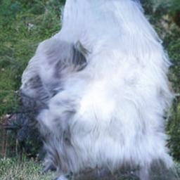
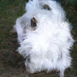
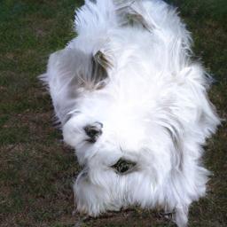
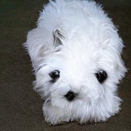
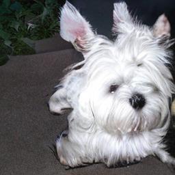
MDT
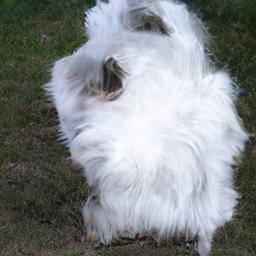
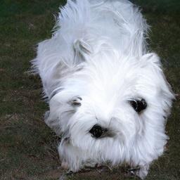
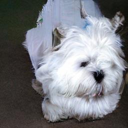
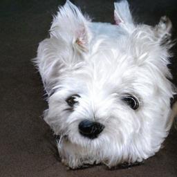
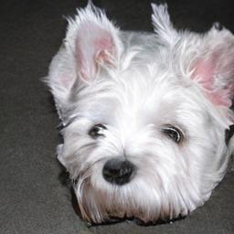
	50k	100k	200k	300k	3000k
Increasing training steps.

\begin{overpic}[width=205.97214pt]{figures/converge_comp.pdf} \put(67.0,79.0){DiT-S/2} \put(67.0,72.0){MDT-S/2} \put(-7.0,18.0){\rotatebox{90.0}{\footnotesize\qquad FID-50K}} \put(30.0,-8.0){Training steps (k)} \put(34.0,22.0){\large$\sim$3.2$\times$} \end{overpic}

(a)

\begin{overpic}[width=205.97214pt]{figures/converge_time_comp.pdf} \put(67.0,79.0){DiT-S/2} \put(67.0,72.0){MDT-S/2} \put(30.0,-7.0){Training times (days)} \put(32.0,20.0){\large$\sim$3.0$\times$} \end{overpic}

(b)

Figure 1: Top: Visualized example of MDT/DiT [31] along with training steps. Down: learning progress comparison between DiT and MDT w.r.t. training steps/times on 8 A100 GPUs. MDT has about 3$\times$ faster learning speed than DiT while achieving superior FID scores.

1 Introduction

Diffusion probabilistic models (DPMs) [10, 34] have been at the forefront of recent advances in image-level generative models, often surpassing the previously state-of-the-art (SoTA) generative adversarial networks (GANs) [4, 50, 33]. Additionally, DPMs have demonstrated their success in numerous other applications, including text-to-image generation [34] and speech generation [21]. DPMs adopt a time-inverted Stochastic Differential Equation (SDE) to gradually map a Gaussian noise into a sample by multiple time steps, with each step corresponding to a network evaluation. In practice, generating a sample is time-consuming due to the thousands of time steps required for the SDE to converge. To address this issue, various generation sampling strategies [18, 28, 37] have been proposed to accelerate the inference speed. Nevertheless, improving the training speed of DPMs is less explored but highly desired. Training of DPMs also unavoidably requires a large number of time steps to ensure the convergence of SDEs, making it very computationally expensive, especially in this era where large-scale models [10, 31] and data [8, 40, 13] are often used to improve generation performance.

In this work, we first observe that DPMs often struggle to learn the associated relations among object parts in an image. This leads to its slow learning process during training. Specifically, as illustrated by fig:converge_comp, the classical DPM, DDPM [18] with DiT [31] as backbone, has learned the shape of a dog at the 50k-th training step, then learns its one eye and mouth until at the 200k-th step while missing another eye. Also, the relative position of two ears is not very accurate even at the 300k-th step. This learning process reveals that DPMs fail to learn the associated relations among semantic parts and indeed independently learn each semantic. The reason behind this phenomenon is that DPMs maximize the log probability of real data by minimizing the per-pixel prediction loss, which ignores the associated relations among object parts in an image, thus resulting in their slow learning progress.

Inspired by the above observation, we propose an effective Masked Diffusion Transformer (MDT) to improve the training efficiency of DPMs. MDT proposes a mask latent modeling scheme designed for transformer-based DPMs to explicitly enhance contextual learning ability and improve the associated relation learning among semantics in an image. Specifically, following [34, 31], MDT operates the diffusion process in the latent space to save computational cost. It masks certain image tokens, and designs an asymmetric masking diffusion transformer (AMDT) to predict masked tokens from unmasked ones in a diffusion generation manner. To this end, AMDT contains an encoder, a side-interpolater and a decoder. The encoder and decoder modify the transformer block in DiT [31] via inserting global and local token position information to help predict masked tokens. The encoder only processes unmasked tokens during training while handling all tokens during inference as there are no masks. So to ensure decoder always processes all tokens for training prediction or inference generation, a side-interpolater implemented by a small network aims to predict masked tokens from encoder output during training, and it is removed during inference.

By this masking latent modeling scheme, our MDT can reconstruct full information of an image from its contextual incomplete input, learning the associated relations among semantics in an image. As shown in  fig:converge_comp, MDT typically generates two eyes (and two ears) of the dog at almost the same training steps, indicating that it correctly learns the associated semantics of an image by utilizing the mask latent modeling scheme. In contrast, DiT [31] cannot easily synthesize a dog with the correct semantic relations among its parts. This comparison shows the superior relation modeling and faster learning ability of MDT over DiT. Experimental results demonstrate that MDT achieves superior performance on the image synthesis task, and set the new SoTA on class-conditional image synthesis on the ImageNet dataset, as shown in fig:sample and tab:sota_comp. MDT also enjoys about 3$\times$ faster learning progress during training than the SoTA DPMs, namely DIT, as demonstrated by fig:converge_comp and tab:ditvsmdt. We hope our work can inspire more works on speeding up the diffusion training process with unified representation learning.

The main contributions are summarised as follows:

• Our proposed masked diffusion transformer introduces an effective mask latent modeling scheme into DPMs and also accordingly designs an asymmetric masking diffusion transformer. Our method is the first one that aims to explicitly enhance contextual learning ability and improve the relation learning among image semantics for DPMs.

• Experiments show that our masked diffusion transformer enjoys higher performance on image synthesis and greatly improves the learning progress during training. It achieves the new SoTA for image synthesis.

Figure 2: Visualization of images generated by the MDT-XL/2.

2 Related works

2.1 Diffusion Probabilistic models

Diffusion probabilistic model (DPM) [18, 10], also known as score-based model [44, 45], is a competitive approach for image synthesis. DPMs begin by using an evolving Stochastic Differential Equation (SDE) to gradually add Gaussian noise into real data, transforming a complex data distribution into a Gaussian distribution. Then, it adopts a time-inverted SDE to gradually map a Gaussian noise into a sample by multiple steps. At each sampling time step, a network is utilized to generate the sample along the gradient of the log probability, also known as the score function [46]. The iterative nature of diffusion models can result in high training and inference costs. Efficient sampling strategies [18, 28, 37, 20, 42], latent space diffusion [34, 47], and multi-resolution cascaded generation [19] have been proposed to reduce the inference cost. Additionally, some training schemes [11, 2] are introduced to improve the diffusion model training, approximate maximum likelihood training [43, 30, 24], training loss weighting [23, 22]. In contrast to them optimizing the diffusion training process, we identify the lack of contextual modeling ability in diffusion models. To address this, we propose the mask latent modeling scheme as a complementary approach to enhancing the contextual representation of diffusion models, which is orthogonal to existing diffusion training schemes.

\begin{overpic}[width=433.62pt]{figures/overall.pdf} \end{overpic}

Figure 3: The overall framework of Masked Diffusion Transformer (MDT). Solid/dotted line indicates the training/inference process for each time step. Masking and side-interpolater are only used during training and are removed during inference.

2.2 Networks for Diffusion Models

The UNet-like [35] network, enhanced by spatial self-attention [38, 48] and group normalization [51] is firstly used for diffusion models [18]. Several design improvements, adding more attention heads, BigGAN [4] residual block, and adaptive group normalization, are proposed in[10] to further enhance the generation ability of the UNet. Recently, due to the broad applicability of transformer networks, several works have attempted to utilize the vision transformer (ViT) structure for diffusion models [52, 1, 31]. GenViT [52] demonstrates that ViT is capable of image generation but has inferior performance compared to UNet. U-ViT [1] improves ViT by adding long-skip connections and convolutional layers, achieving competitive performance with that of UNet. DiT [31] verifies the scaling ability of ViT on large model sizes and feature resolutions. Our MDT is orthogonal to these diffusion networks as it focuses on contextual representation learning. Moreover, the position-aware designs in MDT reveal that the mask latent modeling scheme benefits from a stronger diffusion network. We will explore further to release the potential of these networks with MDT.

2.3 Mask Modeling

Mask modeling has been proven to be effective in both recognition learning [9, 16, 14] and generative modeling [32, 7]. In the natural language processing (NLP) field, mask modeling was first introduced to enable representation pretraining [9, 32] and language generation [5]. Subsequently, it also proved feasible for vision recognition [3] and generation [53, 7, 15] tasks. In vision recognition, pretraining schemes that utilize mask modeling enable good representation quality [54], scalability [16] and faster convergence [14]. In generative modeling, following the bi-directional generative modeling in NLP, MaskGIT [7] and MUSE [6] use the masked generative transformer to predict randomly masked image tokens for image generation. Similarly, VQ-Diffusion [15] presents a mask-replace diffusion strategy to generate images. In contrast, our MDT aims to enhance the contextual representation of the denoising diffusion transformer [31] with mask latent modeling. This preserves the detail refinement ability of denoising diffusion models by maintaining the diffusion process during inference. To ensure that the mask latent modeling in MDT focuses on representation learning instead of reconstruction, we propose an asymmetrical structure in mask modeling training. As an extra benefit, it enables lower training costs than masked generative models because it skips the masked patches in training instead of replacing masked input patches with a mask token.

3 Revisitation of Diffusion Probabilistic Model

For diffusion probabilistic models [10, 41], such as DDPM [18] and DDIM [42], training involves a forward noising process and a reverse denoising process. In the forward noising process, Gaussian noise $\epsilon\sim\mathcal{N}(0,\mathbf{I})$ is gradually added to the real sample $x_{0}$ via a discrete SDE of formulation $q(x_{t},x_{0})=\sqrt{\bar{\alpha}_{t}}x_{0}+\epsilon\sqrt{1-\bar{\alpha}_{t}}$, where $\bar{\alpha}_{t}$ denotes the noise magnitude. If the time step $t$ is large, $x_{t}$ would be a Gaussian noise. Similarly, the reverse denoising process is a discrete SDE that gradually maps a Gaussian noise into a sample. At each time step, given $x_{t}$, it predicts the next reverse step $p_{\theta}(x_{t-1}|x_{t})=\mathcal{N}(x_{t-1};\mu_{\theta}(x_{t},t),\Sigma_{\theta}(x_{t},t))$ via a network. The network is trained by optimizing the variational lower-bound $L_{\text{vlb}}$ of $p_{\theta}(x_{0})$  [41], where $L_{\text{vlb}}=-\log p_{\theta}(x_{0}|x_{1})+\sum_{t}D_{KL}(q(x_{t-1}|x_{t},x_{0})||p_{\theta}(x_{t-1}|x_{t}))$. Following [30, 31], we obtain $\Sigma_{\theta}(x_{t},t)$ by optimizing $L_{\text{vlb}}$, and we reparameterize $\mu_{\theta}(x_{t},t)$ as a noise prediction network $\epsilon_{\theta}(x_{t},t)$ and train it with a simple mean-squared error loss, $L_{\text{simple}}=||\epsilon-\epsilon_{\theta}(x_{t},t)||^{2}$, where $\epsilon$ is the ground truth Gaussian noise. During inference, one can sample a Gaussian noise and then gradually reverses to a sample $x_{0}$.

Same as [30, 31], we train the diffusion model conditioned with class label $c$, $p_{\theta}(x_{t-1}|x_{t},c)$. By default, we use class-conditioned image generation in our experiments.

4 Masked Diffusion Transformer

4.1 Overview

As shown in fig:converge_comp, DPMs with DiT backbone exhibit slow training convergence due to the slowly learning of the associated relations among semantics in an image. To relieve this issue, we propose Masked Diffusion Transformer (MDT), which introduces a mask latent modeling scheme to explicitly enhance contextual learning ability and to improve the capability of establishing associated relations among different semantics in an image. To this end, as depicted in in fig:overall, MDT consists of 1) a latent masking operation to mask the input image in the latent space, and 2) an asymmetric masking diffusion transformer that performs vanilla diffusion process as DPMs, but with masked input. To reduce computational costs, MDT follows LatentDiffusion [34] to perform generative learning in the latent space instead of raw pixel space.

In the training phase, MDT first encodes an image into a latent space with a pre-trained VAE encoder [34]. The latent masking operation in MDT then adds Gaussian noise into the image latent embedding, patchifies the resulting noisy latent embedding into a sequence of tokens, and masks certain tokens. The remaining unmasked tokens are fed into the asymmetric masking diffusion transformer which contains an encoder, a side-interpolater, and a decoder to predict the masked tokens from the unmasked ones. During inference, MDT replaces the side-interpolater with a position embedding adding operation. MDT takes the latent embedding of a Gaussian noise as input to generate the denoised latent embedding, which is then passed to a pre-trained VAE decoder [34] for image generation.

The above masking latent modeling scheme in the training phase forces the diffusion model to reconstruct full information of an image from its contextual incomplete input. Thereby, the model is encouraged to learn the relations among image latent tokens, particularly the associated relations among semantics in an image. For example, as illustrated in fig:overall, the model should first well understand the correct associated relations among small image parts (tokens) of the dog image. Then, it should generate the masked “eye” tokens by using other unmasked tokens as contextual information. Furthermore, fig:converge_comp shows that MDT often learns to generate the associated semantics of an image at nearly the same pace, such as the generation of the two eyes (two ears) of the dog at the almost same training step. While DiT [31] (DDPM with transformer backbone) learns to generate one eye (one ear) initially and then learns to generate another eye (ear) after roughly 100k training steps. This demonstrates the superior learning ability of MDT over DiT in terms of the associated relation learning of image semantics.

In the following parts, we will introduce the two key components of MDT, 1) a latent masking operation, and 2) an asymmetric masking diffusion transformer.

4.2 Latent Masking

Following the Latent diffusion model (LDM) [34], MDT performs generation learning in the latent space instead of raw pixel space to reduce computational costs. In the following, we briefly recall LDM and then introduce our latent masking operation on the latent input.

Latent diffusion model (LDM). LDM employs a pre-trained VAE encoder E to encode an image $v\in\mathbb{R}^{3\times H\times W}$ to a latent embedding $z=\textbf{E}(v)\in\mathbb{R}^{c\times h\times w}$. It gradually adds noise to $z$ in the forward process and then denoises to predict $z$ in the reverse process. Finally, LDM uses a pre-trained VAE decoder D to decode $z$ into a high-resolution image $v=\textbf{D}(z)$. Both VAE encoder and decoder are kept fixed during training and inference. Since $h$ and $w$ are smaller than $H$ and $W$, performing the diffusion process in the low-resolution latent space is more efficient compared to the pixel space. In this work, we adopt the efficient diffusion process of LDM.

Latent masking operation. Now we present our masking scheme on latent input. During training, we first add Gaussian noise to the latent embedding $z$ of an image. Then following [31], we divide the noisy embedding $z$ into a sequence of $p\times p$-sized tokens, and concatenate them to a matrix $u\in\mathbb{R}^{d\times N}$, where $d$ is the channel number and $N$ is the number of tokens. Next, we randomly mask tokens with a ratio $\rho$ and concatenate the remaining tokens as $\hat{u}\in\mathbb{R}^{d\times\hat{N}}$, where $\hat{N}=\rho N$. Accordingly, we can create a binary mask $M\in\mathbb{R}^{N}$ in which one (zero) denotes the masked (unmasked) tokens. Finally, we feed the unmasked tokens $\hat{u}$ into our diffusion model for processing. We only use unmasked tokens $\hat{u}$, because 1) The model should focus on learning semantics instead of predicting the masked tokens. As shown in sec:abl, it achieves better performance than replacing the masked tokens with a learnable mask token and then processing all tokens like [3, 7, 6] ; 2) It saves the training cost compared to processing all $N$ tokens.

\begin{overpic}[width=433.62pt]{figures/block.pdf} \end{overpic}

Figure 4: The asymmetric masking diffusion transformer in MDT. We modify the DiT [31] by adding a side-interpolater, local relative positional bias, and learnable global position embeddings. The conditional scheme is omitted for simplicity.

4.3 Asymmetric Masking Diffusion Transformer

We introduce our asymmetric masking diffusion transformer for performing joint training of mask latent modeling and diffusion process. As shown in fig:block, it consists of three components: an encoder, a side-interpolater and a decoder, each of which is described in detail at below.

Position-aware encoder and decoder. In MDT, predicting the masked latent tokens from the unmasked tokens requires the position relations of all tokens. To enhance the position information in the model, we propose positional-aware encoder and decoder that facilitate the learning of the masked latent tokens. Specifically, the encoder and decoder tailor the standard DiT block via adding two kinds of token position information, and respectively contain $N_{1}$ and $N_{2}$ tailored blocks.

Firstly, as illustrated in fig:block, the encoder adds the conventional learnable global position embedding into the noisy latent embedding input. Similarly, the decoder also introduces the learnable position embedding into its input but with different approaches in the training and inference phases. During training, the side-interpolater already uses the learnable global position embedding as introduced below, which can deliver the global position information to the decoder. During inference, since the side interpolater is discarded (see below), the decoder explicitly adds the position embedding into its input to enhance positional information.

Secondly, as shown in fig:block, the encoder and decoder add a local relative positional bias [26] to each head in each block when computing the attention score of the self-attention [49]:

$$\mbox{Attention}(Q,K,V)=\mbox{Softmax}\left(\frac{QK^{\top}}{\sqrt{d_{k}}}+B_{r}\right)V,$$

where $Q$, $K$, and $V$ respectively denote the query, key and value in self-attention module, $d_{k}$ is the dimension of the key, and $B_{r}\in\mathbb{R}^{N\times N}$ is the relative positional bias that is selected by the relative positional difference $\Delta$ between the $i$-th position and other positions, $B_{r}(i,\Delta)$. The learnable mapping $B_{r}$ is updated during training. The local relative positional bias helps to capture the relative relations among tokens, facilitating the masking latent modeling.

The encoder takes the unmasked noisy latent embedding provided by our latent masking operation, and feeds its output into the side-interpolater/decoder during training/inference. For decoder, its input is the output of side-interpolater for training or the combination of the encoder output and the learnable position embedding for inference. Since during training, the encoder and decoder respectively handle unmasked tokens and full tokens, we call our model as the “asymmetric” model.

Side-interpolater. As shown in Fig. 3, during training, for efficiency and better performance, the encoder only processes the unmasked tokens $\hat{u}$. While in the inference phase, the encoder handles all tokens $u$ due to the lack of masks. This means that there is a big difference in encoder output (decoder input) during training and inference, at least in terms of token number. To ensure decoder always processes all tokens for training prediction or inference generation, side-interpolater implemented by a small network aims to predict masked tokens from encoder output during training and would be removed during inference.

In the training phase, the encoder processes the unmasked tokens to obtain its output token embedding $\hat{q}\in\mathbb{R}^{d\times\hat{N}}$. Then as shown in Fig. 3, the side-interpolater first fills the masked positions, indicated by the mask $M$ defined in Sec. 4.2, by a shared learnable mask token, and also adds a learnable positional embedding to obtain embedding $q\in\mathbb{R}^{d\times N}$. Next, we use a basic block of the encoder to process $q$ to predict an interpolated embedding $\hat{k}$. The tokens in $\hat{k}$ denote the predicted tokens. Finally, we use a masked shortcut connection to combine prediction $\hat{k}$ and $q$ as $k=M\cdot q+(1-M)\cdot\hat{k}$. In summary, for masked tokens, we use the prediction by side-interpolater; for unmasked tokens, we still adopt the corresponding tokens in $q$. This can 1) boost the consistency between training and inference phases, 2) eliminates the mask-reconstruction process in the decoder.

Since there are no masks during inference, the side-interpolater is replaced by a position embedding operation which adds the learnable position embeddings of side-interpolater which is learned during training. This ensures the decoder always processes all tokens and uses the same learnable position embeddings for training prediction or inference generation, thus having better image generation performance.

4.4 Training

During training, we feed both full latent embedding $u$ and the masked latent embedding $\hat{u}$ to the diffusion model, since we observe that only using masked latent embedding makes the model focus too much on masked region reconstruction while ignoring the diffusion training. The training objectives for full/masked latent inputs both follow the description in sec:ddpm. Due to the asymmetrical masking structure, the extra costs for using masked latent embedding is small. This is also demonstrated by fig:converge_comp which shows that MDT still achieves about 3$\times$ faster learning progress than previous SoTA DiT in terms of total training hours.

Method	Cost(Iter$\times$BS)	FID$\downarrow$	sFID$\downarrow$	IS$\uparrow$	Prec.$\uparrow$	Rec.$\uparrow$
DCTrans.[29]	-	36.51	-	-	0.36	0.67
VQVAE-2[33]	-	31.11	-	-	0.36	0.57
VQGAN[12]	-	15.78	78.3	-	-	-
BigGAN-deep[4]	-	6.95	7.36	171.4	0.87	0.28
StyleGAN[39]	-	2.30	4.02	265.12	0.78	0.53
Impr. DDPM[30]	-	12.26	-	-	0.70	0.62
MaskGIT[7]	1387k$\times$256	6.18	-	182.1	0.80	0.51
CDM[19]	-	4.88	-	158.71	-	-
ADM[10]	1980k$\times$256	10.94	6.02	100.98	0.69	0.63
LDM-8[34]	4800k$\times$64	15.51	-	79.03	0.65	0.63
LDM-4	178k$\times$1200	10.56	-	103.49	0.71	0.62
DiT-XL/2[31]	7000k$\times$256	9.62	6.85	121.50	0.67	0.67
MDT	2500k$\times$256	7.41	4.95	121.22	0.72	0.64
MDT	3500k$\times$256	6.46	4.92	131.70	0.72	0.63
MDT	6500k$\times$256	6.23	5.23	143.02	0.71	0.65
ADM-G[10]	1980k$\times$256	4.59	5.25	186.70	0.82	0.52
ADM-G, U	1980k$\times$256	3.94	6.14	215.84	0.83	0.53
LDM-8-G[34]	4800k$\times$64	7.76	-	209.52	0.84	0.35
LDM-4-G	178k$\times$1200	3.60	-	247.67	0.87	0.48
U-ViT-G [1]	300k$\times$1024	3.40	-	-	-	-
DiT-XL/2-G[31]	7000k$\times$256	2.27	4.60	278.24	0.83	0.57
MDT-G	2500k$\times$256	2.15	4.52	249.27	0.82	0.58
MDT-G	3500k$\times$256	2.02	4.46	263.77	0.82	0.60
MDT-G	6500k$\times$256	1.79	4.57	283.01	0.81	0.61

Table 1: Comparison with existing methods on class-conditional image generation with the ImageNet 256$\times$256 dataset. -G denotes the results with classifier-free guidance [20]. Results of MDT-XL/2 model are given for comparison. Compared results are obtained from their papers.

5 Experiments

5.1 Implementation

We give the implementation details of MDT, including model architecture, training details, and evaluation metrics.

Model architecture. We follow DiT [31] to set the total block number ( $N_{1}+N_{2}$), token number, and channel numbers of the diffusion transformer of MDT. As DiT reveals stronger synthesis performance when using a smaller patch size, we also use a patch size $p$=2 by default, denoted by MDT-/2. Moreover, We also follow DiT’s parameters to design MDT for getting its small-, base-, and xlarge-sized model, denoted by MDT-S/B/XL. Same as LatentDiffusion [34] and DiT, MDT adopts the fixed VAE provided by the Stable Diffusion to encode/decode the image/latent tokens by default. The VAE encoder has a downsampling ratio of $1/8$, and a feature channel dimension of 4,  an image of size 256$\times$256$\times$3 is encoded into a latent embedding of size 32$\times$32$\times$4.

Training details. Following [31], all models are trained by AdamW [27] optimizer of 3e-4 learning rate, 256 batch size, and without weight decay on ImageNet [8] with an image resolution of 256$\times$256. We set the mask ratio as 0.3 and $N_{2}=2$. Following the training settings in DiT, we set the maximum step in training to 1000 and use the linear variance schedule with a range from $10^{-4}$ to $2\times 10^{-2}$. Other settings are also aligned with DiT.

Evaluation. We evaluate models with commonly used metrics, Fre’chet Inception Distance (FID) [17], sFID [29], Inception Score (IS) [36], Precision and Recall [25]. The FID is used as the major metric as it measures both diversity and fidelity. sFID improves upon FID by evaluating at the spatial level. As a complement, IS and Precision are used for measuring fidelity, and Recall is used to measure diversity. For fair comparisons, we follow [31] to use the TensorFlow evaluation suite from ADM [10] and report FID-50K with 250 DDPM sampling steps. Unless specified otherwise, we report the FID scores without the classifier-free guidance [20].

Method	Image Res.	Training Steps (k)	FID-50K$\downarrow$
DiT-S/2	256$\times$256	400	68.40
MDT-S/2	256$\times$256	300	57.01
MDT-S/2	256$\times$256	400	53.46
MDT-S/2	256$\times$256	2000	44.14
MDT-S/2	256$\times$256	3500	41.37
DiT-B/2	256$\times$256	400	43.47
MDT-B/2	256$\times$256	400	34.33
MDT-B/2	256$\times$256	3500	20.45
DiT-XL/2	256$\times$256	400	19.47
DiT-XL/2	256$\times$256	2352	10.67
DiT-XL/2	256$\times$256	7000	9.62
MDT-XL/2	256$\times$256	400	16.42
MDT-XL/2	256$\times$256	1300	9.60
MDT-XL/2	256$\times$256	3500	6.65

Table 2: Comparison between DiT [31] and MDT under different model sizes and training steps on ImageNet 256$\times$256. DiT results are obtained from DiT reported results.

5.2 Comparison Results

Performance comparison. tab:ditvsmdt compares our MDT with the SoTA DiT under different model sizes. It is evident that MDT achieves higher FID scores for all model scales with fewer training costs. The parameters and inference cost of MDTs are similar to DiT, since the extra modules in MDT are negligible as introduced in sec:mdt_method. For small models, MDT-S/2 trained with 300k steps outperforms the DiT-S/2 trained with 400k steps by a large margin on FID (57.01 vs. 68.40). More importantly, MDT-S/2 trained with 2000k steps achieves similar performance with a larger model DiT-B/2 trained with a similar computational budget. For the largest model, MDT-XL/2 trained with 1300k steps outperforms DiT-XL/2 trained with 7000k steps on FID (9.60 vs. 9.62), achieving about 5$\times$ faster training progress.

We also compare the class-conditional image generation performance of MDT with existing methods in tab:sota_comp. To make fair comparisons with DiT, we also use the EMA weights of VAE decoder in this table. Under class-conditional settings, MDT with half training iterations outperforms DiT by a large margin, 6.83 vs 9.62 in FID. Following previous works [34, 10, 31, 1], we utilize an improved classifier-free guidance [20] with a power-cosine weight scaling to trade off between precision and recall during class-conditional sampling. MDT achieves superior performance over previous SoTA DiT and other methods with the FID score of 1.81, setting a new SoTA for class-conditional image generation. Similar to DiT, we never observe the model has saturated FID scores when continuing training.

Convergence speed. fig:converge_comp compares the performance of the DiT/S-2 baseline and MDT/S-2 under different training steps and training time on 8$\times$A100 GPUs. Because of the stronger contextual learning ability, MDT achieves better performance with faster generation learning speed. MDT enjoys about 3$\times$ faster learning speed in terms of both training steps and training time. For example, MDT-S/2 trained with about 33 hours (400k steps) achieves superior performance than DiT-S/2 trained with about 100 hours (1500k steps). This reveals that contextual learning is vital for faster generation learning of diffusion models.

Mask Ratio	FID$\downarrow$	sFID$\downarrow$	IS$\uparrow$	Precision$\uparrow$	Recall$\uparrow$
0.1	51.60	10.23	26.65	0.44	0.60
0.2	51.44	10.09	26.75	0.44	0.58
0.3	50.26	10.08	27.61	0.45	0.60
0.4	50.88	10.21	27.44	0.45	0.60
0.5	51.57	9.92	27.14	0.44	0.60
0.6	53.20	10.36	26.55	0.44	0.61
0.7	52.90	10.03	26.51	0.44	0.61
0.8	53.73	10.15	25.55	0.43	0.61

Table 3: Effect of different masking ratios. MDT-S/2 trained with 600k iterations.

5.3 Ablation

In this part, we conduct ablation to verify the designs in MDT. We report the results of MDT-S/2 model and use FID-50k as the evaluation metric unless otherwise stated.

Decoder pos.	FID$\downarrow$	sFID$\downarrow$	IS$\uparrow$	Precision$\uparrow$	Recall$\uparrow$
Last0	51.05	9.97	27.31	0.44	0.60
Last1	50.96	9.90	27.63	0.45	0.60
Last2	50.26	10.08	27.61	0.45	0.60
Last4	51.67	10.12	26.91	0.45	0.60
Last6	52.64	10.36	26.46	0.44	0.60

Table 4: Effect of position of side-interpolater. MDT-S/2 models contain 12 blocks and are trained with 600k iterations.

Asymmetric stru.	FID-50k$\downarrow$
$\times$	51.56
$\checkmark$	50.26

(a) Effect of asymmetric masking structure.

Side-interpolater	FID-50k$\downarrow$
$\times$	51.60
$\checkmark$	50.26

(b) Effect of side-interpolater.

Masked shortcut	FID-50k$\downarrow$
$\times$	50.91
$\checkmark$	50.26

(c) Effect of masked shortcut.

Latent type	FID-50k$\downarrow$
Full+Masked	50.26
Full	52.30
Masked	76.63

(d) Using full/masked latent under aligned cost.

Sup. parts	FID-50k$\downarrow$
All	50.26
Masked	58.35

(e) Supervision on token parts.

Number	FID-50k$\downarrow$
1	50.26
2	51.77
3	51.96

(f) Number of blocks in side-interpolator.

IS Pos. embed.	FID-50k$\downarrow$
$\times$	51.58
$\checkmark$	50.26

(g) Effect of positional embeddings in SI.

Learnable pos.	FID-50k$\downarrow$
$\times$	50.80
$\checkmark$	50.26

(h) Effect of learnable positional embeddings.

Relative pos. bias	FID-50k$\downarrow$
$\times$	53.56
$\checkmark$	50.26

(i) Effect of relative positional bias.

Table 5: Ablation study on MDT-S/2. Models are trained for 600k iterations.

Masking ratio. The masking ratio determines the number of input patches that can be processed during training. We give the comparison of using different masking ratios in tab:maskratio. The best masking ratio for MDT-S/2 is 30%, which is quite different from the masking ratio used for recognition models, e.g. 75% masking ratio in MAE [16]. We assume that the image generation requires learning more details from more patches for high-quality synthesis, while recognition models only need the most essential patches to infer semantics.

Asymmetric vs. Symmetric architecture in masking. Unlike the masked generation works [7, 6], MaskGIT, that utilize the masking scheme to generate images, MDT focuses on improving diffusion models with contextual learning ability via the masking latent modeling. Therefore, we use an asymmetric architecture to only process the unmasked tokens in the diffusion model encoder. We compare the asymmetric architecture in MDT and the symmetrical architecture [7] that processes full input with masked tokens replaced by a learnable mask token. As shown in tab:asymmetric_mask, the asymmetric architecture in MDT has an FID of 50.26, outperforming the FID of 51.56 achieved by the symmetric architecture. The asymmetric architecture further reduces the training cost and allows the diffusion model to focus on learning contextual information instead of reconstructing masked tokens.

Full and masked latent tokens. In MDT, both the full and masked latent embeddings are fed into the diffusion model during training. In comparison, we give the results trained by only using full/masked latent embeddings as shown in tab:used_latent, where the computational cost is aligned for fair comparisons. Trained with both full and masked latent leads to clear gain over two competitors. While using only the masked latent embeddings results in slow convergence, which we attribute to the training/inference inconsistency as the inference in MDT is a diffusion process instead of the masked reconstruction process.

Loss on all tokens. By default, we calculate the loss on both masked and unmasked latent embeddings. In comparison, mask modeling for recognition models commonly calculates loss on masked tokens [16, 3]. tab:mask_sup shows that calculating the loss on all tokens is much better than on masked tokens. We assume that this is because generative models require stronger consistency among patches than recognition models do, since details are vital for high-quality image synthesis.

Effect of side-interpolater. The side-interpolater in MDT predicts the masked tokens, allowing the diffusion model to learn more semantics and maintain consistency in decoder inputs during training and inference. We compare the performance with/without the side-interpolater in tab:side_interpolater, and observe a gain of 1.34 in FID when using the side-interpolater, proving its effectiveness.

Masked shortcut in side-interpolater. The masked shortcut ensures that the side-interpolater only predicts the masked tokens from unmasked ones. tab:masking_shortcut shows that using the masked shortcut enhances the FID from 50.91 to 50.26, indicating that restricting side-interpolater to only predict masked tokens helps the diffusion model achieve stronger performance.

Side-interpolater position. To meet the high-quality image generation requirements of the diffusion model, the side-interpolater is placed in the middle of the network instead of the end of the network in recognition models [16, 3]. tab:decoder_pos, presents the comparison of placing the side-interpolater at different positions of the MDT-S model with 12 blocks. The results show that placing the side-interpolater before the last two blocks achieves the best FID score, whereas placing it at the end of the network like recognition models impairs the performance. Placing the side-interpolater at the early stages of the network also harm the performance, indicating the mask latent modeling is beneficial to most stages in the diffusion models.

Block number in side-interpolater. We compare the performance of different numbers of blocks in the side-interpolater in tab:num_block_si. The default setting of 1 block achieves the best performance, and the FID worsens with an increase in block number. This result is consistent with our motivation that side-interpolater should not learn too much information other than interpolating the masked representations.

Positional-aware enhancement. To further release the potential of mask latent modeling, we enhance the DiT baseline with stronger positional awareness ability, learnable positional embeddings and the relative positional bias in basic blocks. tab:pos_embed_si shows the positional embeddings in side-interpolater improves the FID from 51.58 to 50.26, indicating the positional embedding is vital for the side-interpolater. Also, enables the training of positional embeddings brings the gain in FID as revealed in tab:learn_pos. In tab:rel_bias, the relative positional bias in the basic blocks significantly improves the FID from 53.56 to 50.26, showing the relative positional modeling ability is essential for diffusion models to obtain the contextual representation ability and generate high-quality images. Therefore, the positional awareness ability in diffusion model structure is required to accompany the masked latent modeling, playing a key role in improving performance.

6 Conclusion

This work proposes a masked diffusion transformer to enhance the contextual representation and improve the relation learning among image semantics for DPMs. We introduce an effective mask latent modeling scheme into DPMs and also accordingly designs an asymmetric masking diffusion transformer. Experiments show that our masked diffusion transformer enjoys higher performance on image synthesis and largely improves the learning progress during training, achieving the new SoTA for image synthesis on the ImageNet dataset.

Masked
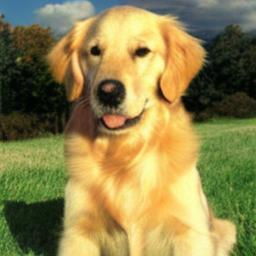
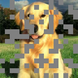
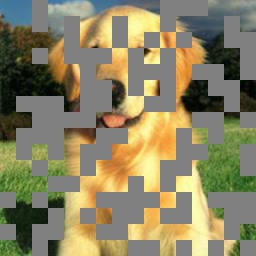
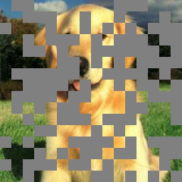
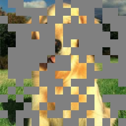
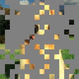
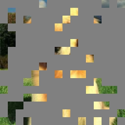
Inpainted
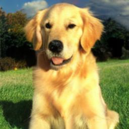
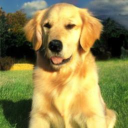
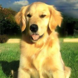
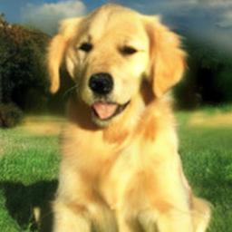
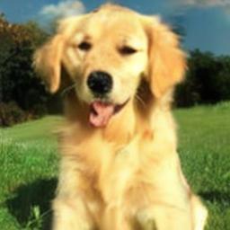
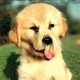
Masked
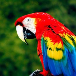
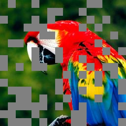
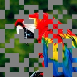
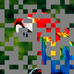
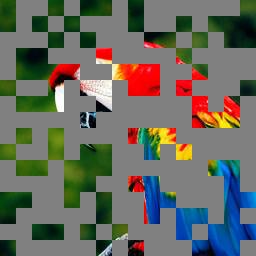
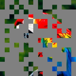
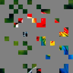
Inpainted
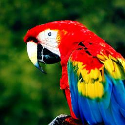
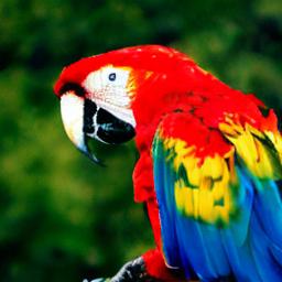
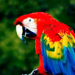
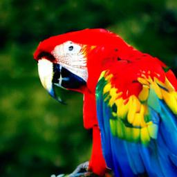
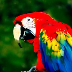
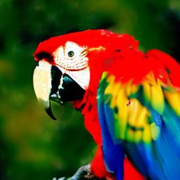
	Original	mask=30%	mask=40%	mask=50%	mask=60%	mask=70%	mask=80%

Figure 5: Inpainting under different masked ratios using MDT-XL/2.

Appendix A Model Details

Network configurations. We follow the network configurations described in DiT [31] to set the total block number ( $N_{1}+N_{2}$), token number, and channel numbers for the masked diffusion transformer of MDT. The configurations of MDT models are given in tab:model_config. Following DiT, the MDT has models with different sizes, denoted by S/B/XL.

Network parameters and costs. The network parameters and training costs for MDT under different model scales are listed in tab:model_config. In comparison to DiT baselines, MDT introduces a negligible extra inference parameters and costs.

Size	Layers	Dim.	Head Num.	Param. (M)	FLOSs (G)
Network configurations of MDT models.
S	12	384	6	33.1	6.07
B	12	768	12	130.8	23.02
XL	28	1152	16	675.8	118.69
Network configurations of DiT baselines.
S	12	384	6	32.9	6.06
B	12	768	12	130.3	23.01
XL	28	1152	16	674.8	118.64

Table 6: Network configurations of MDT models. The configurations are following DiT networks [31]. The layers consist of the layer numbers of encoder and decoder, and the decoder number $N_{2}$ is set to 2 for all models. FLOSs are measured with the latent embedding size of 32$\times$32 and $p$=2. The parameters and FLOSs are measured using the inference model.

Appendix B Comparison of VAE decoders

To ensure fair comparisons with DiT [31], we use both the MSE and EMA versions of pretrained VAE decoders for image sampling. tab:emavsmse shows that the EMA version has slightly better performance than the MSE version. Except for the results in Table 1 of the manuscript that uses the EMA VAE decoder, we use the MSE VAE decoder by default.

Method	Decoder	FID$\downarrow$	sFID$\downarrow$	IS$\uparrow$	Prec.$\uparrow$	Rec.$\uparrow$
MDT	MSE	6.65	5.07	129.47	0.72	0.63
MDT	EMA	6.46	4.92	131.70	0.72	0.63
MDT-G	MSE	2.14	4.45	259.21	0.82	0.59
MDT-G	EMA	2.02	4.46	263.77	0.82	0.60

Table 7: Comparison between the EMA and MSE version of VAE decoders. -G denotes the results with classifier-free guidance.

Appendix C Inpainting with MDT

By default, MDT uses the mask latent modeling during training and becomes the standard diffusion model during inference. When the side-interpolater is kept during inference, MDT naturally enables the image inpainting ability. As shown in fig:inpainting, we utilize different mask ratios on the image and inpaint the masked parts with MDT. Although the MDT model is trained with the mask ratio of 30%, it can easily handle much larger masking ratios, such as 70% mask ratio. We attribute this ability to the combination of our proposed mask latent modeling and the diffusion model.

Appendix D Improved Classifier-free Guidance

The classifier-free guidance sampling [20] enables the trade-off between sample quality and diversity. It achieves this by combining the class-conditional and unconditional estimation:

$$\hat{\epsilon}_{\theta}(x_{t},c)=\epsilon_{\theta}(x_{t})+w\cdot(\epsilon_{\theta}(x_{t},c)-\epsilon_{\theta}(x_{t})),$$

where $\epsilon_{\theta}(x_{t},c)$ is the class-conditional estimation, $\epsilon_{\theta}(x_{t})$ is the unconditional estimation, and $w$ is the guidance scale. Generally, a larger $w$ results in high sample quality by decreasing the diversity. MUSE [6] changes the fixed guidance scale with a linear increasing schedule during sampling, which makes the model samples with more diversity at early steps while samples with higher fidelity at late steps. Inspired by this, we present a power-cosine schedule for the guidance scale during the sampling procedure:

$$w_{t}=\frac{1-\cos{\pi\left(\frac{t}{t_{\text{max}}}\right)^{s}}}{2}w,$$

where $t$ is the time step during sampling, $t_{\text{max}}$ is the maximum sampling step, $w$ is the maximum guidance scale, and $s$ is a factor that controls the increasing speed of the guidance scale. As revealed in fig:powercos, the power-cosine schedule enables a low guidance scale at early steps while quickly increasing the guidance scale at late steps. By increasing $s$, the guidance scale has a slow increase at early steps and a fast increase at late steps. The improved classifier-free guidance sampling equipped with the power-cosine guidance scale schedule enables the model samples with high diversity at early steps and high quality at late steps. In this work, $s$ is set to 4, and the corresponding $w$ is set to 3.8 to ensure the model generates images with high fidelity at late steps.

\begin{overpic}[width=420.61192pt]{figures/powercos.pdf} \put(-5.0,43.0){\large\rotatebox{0.0}{$\frac{w_{t}}{w}$}} \put(50.0,-3.0){\large$\frac{t}{t_{\text{max}}}$} \end{overpic}

Figure 6: The power-cosine scaling schedule for guidance scale in classifier-free guidance with difference $s$. A larger $s$ results in a slower increase of $w$ at early steps and a faster increase at late steps.

Appendix E Visualization

We provide more visualized examples of MDT-XL/2 generated images in fig:samplemore. In fig:inc, we show more visualized examples of MDT-S/2 along with training steps.

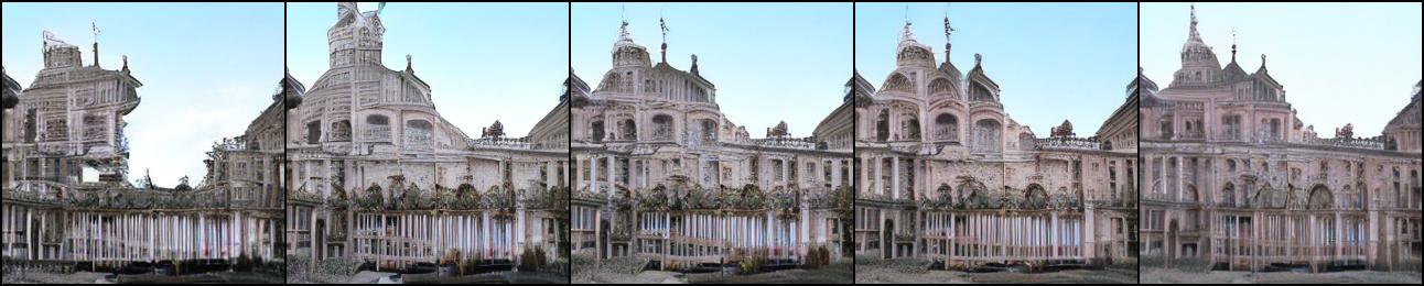
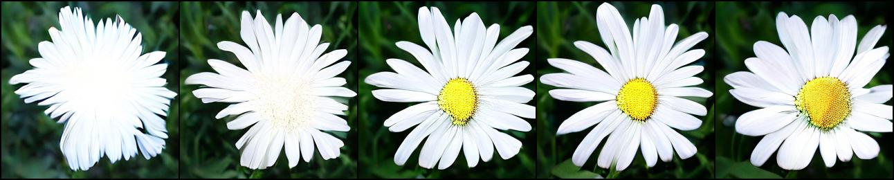
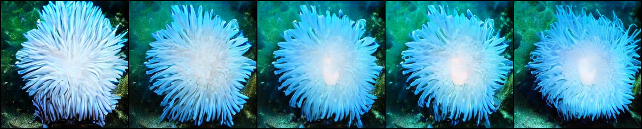
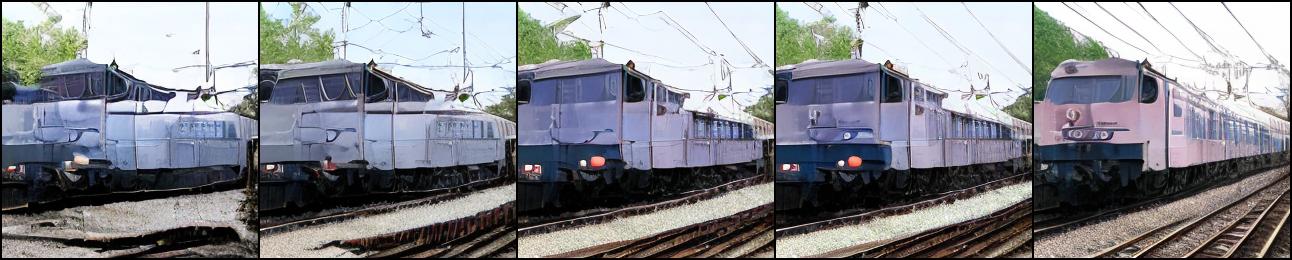
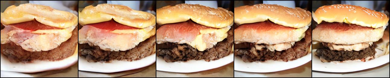
50k	100k	200k	300k	3000k

Figure 7: Visualized example of MDT-S/2 along with training steps.

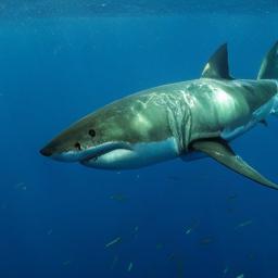
Figure 8: Visualization of images generated by the MDT-XL/2.

References

- [1] Fan Bao, Chongxuan Li, Yue Cao, and Jun Zhu. All are worth words: a vit backbone for score-based diffusion models. arXiv preprint arXiv:2209.12152, 2022.
- [2] Fan Bao, Chongxuan Li, Jiacheng Sun, Jun Zhu, and Bo Zhang. Estimating the optimal covariance with imperfect mean in diffusion probabilistic models. In International Conference on Machine Learning (ICML), 2022.
- [3] Hangbo Bao, Li Dong, and Furu Wei. Beit: Bert pre-training of image transformers. International Conference on Learning Representations (ICLR), 2022.
- [4] Andrew Brock, Jeff Donahue, and Karen Simonyan. Large scale gan training for high fidelity natural image synthesis. International Conference on Learning Representations (ICLR), 2019.
- [5] Tom Brown, Benjamin Mann, Nick Ryder, Melanie Subbiah, Jared D Kaplan, Prafulla Dhariwal, Arvind Neelakantan, Pranav Shyam, Girish Sastry, Amanda Askell, et al. Language models are few-shot learners. Advances in Neural Information Processing Systems (NeurIPS), 33:1877–1901, 2020.
- [6] Huiwen Chang, Han Zhang, Jarred Barber, AJ Maschinot, Jose Lezama, Lu Jiang, Ming-Hsuan Yang, Kevin Murphy, William T Freeman, Michael Rubinstein, et al. Muse: Text-to-image generation via masked generative transformers. arXiv preprint arXiv:2301.00704, 2023.
- [7] Huiwen Chang, Han Zhang, Lu Jiang, Ce Liu, and William T Freeman. Maskgit: Masked generative image transformer. In IEEE Conference on Computer Vision and Pattern Recognition (CVPR), pages 11315–11325, 2022.
- [8] J. Deng, W. Dong, R. Socher, L.-J. Li, K. Li, and L. Fei-Fei. Imagenet: A large-scale hierarchical image database. In IEEE Conference on Computer Vision and Pattern Recognition (CVPR), 2009.
- [9] Jacob Devlin, Ming-Wei Chang, Kenton Lee, and Kristina Toutanova. Bert: Pre-training of deep bidirectional transformers for language understanding. NAACL, 2019.
- [10] Prafulla Dhariwal and Alexander Nichol. Diffusion models beat gans on image synthesis. Advances in Neural Information Processing Systems (NeurIPS), 34:8780–8794, 2021.
- [11] Tim Dockhorn, Arash Vahdat, and Karsten Kreis. Score-based generative modeling with critically-damped langevin diffusion. In International Conference on Learning Representations (ICLR), 2022.
- [12] Patrick Esser, Robin Rombach, and Bjorn Ommer. Taming transformers for high-resolution image synthesis. In IEEE Conference on Computer Vision and Pattern Recognition (CVPR), pages 12873–12883, 2021.
- [13] Shanghua Gao, Zhong-Yu Li, Ming-Hsuan Yang, Ming-Ming Cheng, Junwei Han, and Philip Torr. Large-scale unsupervised semantic segmentation. IEEE Transactions on Pattern Analysis and Machine Intelligence (TPAMI), 2022.
- [14] Shanghua Gao, Pan Zhou, Ming-Ming Cheng, and Shuicheng Yan. Towards sustainable self-supervised learning. arXiv preprint arXiv:2210.11016, 2022.
- [15] Shuyang Gu, Dong Chen, Jianmin Bao, Fang Wen, Bo Zhang, Dongdong Chen, Lu Yuan, and Baining Guo. Vector quantized diffusion model for text-to-image synthesis. In IEEE Conference on Computer Vision and Pattern Recognition (CVPR), pages 10696–10706, 2022.
- [16] Kaiming He, Xinlei Chen, Saining Xie, Yanghao Li, Piotr Dollár, and Ross Girshick. Masked autoencoders are scalable vision learners. In IEEE Conference on Computer Vision and Pattern Recognition (CVPR), pages 16000–16009, 2022.
- [17] Martin Heusel, Hubert Ramsauer, Thomas Unterthiner, Bernhard Nessler, and Sepp Hochreiter. Gans trained by a two time-scale update rule converge to a local nash equilibrium. Advances in Neural Information Processing Systems (NeurIPS), 30, 2017.
- [18] Jonathan Ho, Ajay Jain, and Pieter Abbeel. Denoising diffusion probabilistic models. Advances in Neural Information Processing Systems (NeurIPS), 33:6840–6851, 2020.
- [19] Jonathan Ho, Chitwan Saharia, William Chan, David J Fleet, Mohammad Norouzi, and Tim Salimans. Cascaded diffusion models for high fidelity image generation. Journal of machine learning research (JMLR), 23(47):1–33, 2022.
- [20] Jonathan Ho and Tim Salimans. Classifier-free diffusion guidance. NeurIPS Workshop, 2021.
- [21] Myeonghun Jeong, Hyeongju Kim, Sung Jun Cheon, Byoung Jin Choi, and Nam Soo Kim. Diff-tts: A denoising diffusion model for text-to-speech. In INTERSPEECH, 2021.
- [22] Tero Karras, Miika Aittala, Timo Aila, and Samuli Laine. Elucidating the design space of diffusion-based generative models. In Advances in Neural Information Processing Systems (NeurIPS), 2022.
- [23] Dongjun Kim, Seungjae Shin, Kyungwoo Song, Wanmo Kang, and Il-Chul Moon. Soft truncation: A universal training technique of score-based diffusion model for high precision score estimation. In International Conference on Machine Learning (ICML), 2022.
- [24] Diederik Kingma, Tim Salimans, Ben Poole, and Jonathan Ho. Variational diffusion models. Advances in Neural Information Processing Systems (NeurIPS), 34:21696–21707, 2021.
- [25] Tuomas Kynkäänniemi, Tero Karras, Samuli Laine, Jaakko Lehtinen, and Timo Aila. Improved precision and recall metric for assessing generative models. Advances in Neural Information Processing Systems (NeurIPS), 32, 2019.
- [26] Ze Liu, Yutong Lin, Yue Cao, Han Hu, Yixuan Wei, Zheng Zhang, Stephen Lin, and Baining Guo. Swin transformer: Hierarchical vision transformer using shifted windows. In IEEE International Conference on Computer Vision (ICCV), pages 10012–10022, 2021.
- [27] Ilya Loshchilov and Frank Hutter. Decoupled weight decay regularization. International Conference on Learning Representations (ICLR), 2019.
- [28] Cheng Lu, Yuhao Zhou, Fan Bao, Jianfei Chen, Chongxuan Li, and Jun Zhu. Dpm-solver: A fast ode solver for diffusion probabilistic model sampling in around 10 steps. Advances in Neural Information Processing Systems (NeurIPS), 2022.
- [29] Charlie Nash, Jacob Menick, Sander Dieleman, and Peter W Battaglia. Generating images with sparse representations. International Conference on Machine Learning (ICML), 2021.
- [30] Alexander Quinn Nichol and Prafulla Dhariwal. Improved denoising diffusion probabilistic models. In International Conference on Machine Learning (ICML), pages 8162–8171. PMLR, 2021.
- [31] William Peebles and Saining Xie. Scalable diffusion models with transformers. arXiv preprint arXiv:2212.09748, 2022.
- [32] Alec Radford, Karthik Narasimhan, Tim Salimans, Ilya Sutskever, et al. Improving language understanding by generative pre-training, 2018.
- [33] Ali Razavi, Aaron Van den Oord, and Oriol Vinyals. Generating diverse high-fidelity images with vq-vae-2. Advances in Neural Information Processing Systems (NeurIPS), 32, 2019.
- [34] Robin Rombach, Andreas Blattmann, Dominik Lorenz, Patrick Esser, and Björn Ommer. High-resolution image synthesis with latent diffusion models. In IEEE Conference on Computer Vision and Pattern Recognition (CVPR), pages 10684–10695, 2022.
- [35] Olaf Ronneberger, Philipp Fischer, and Thomas Brox. U-net: Convolutional networks for biomedical image segmentation. In Medical Image Computing and Computer-Assisted Intervention–MICCAI, pages 234–241. Springer, 2015.
- [36] Tim Salimans, Ian Goodfellow, Wojciech Zaremba, Vicki Cheung, Alec Radford, and Xi Chen. Improved techniques for training gans. Advances in Neural Information Processing Systems (NeurIPS), 29, 2016.
- [37] Tim Salimans and Jonathan Ho. Progressive distillation for fast sampling of diffusion models. International Conference on Learning Representations (ICLR), 2022.
- [38] Tim Salimans, Andrej Karpathy, Xi Chen, and Diederik P Kingma. Pixelcnn++: Improving the pixelcnn with discretized logistic mixture likelihood and other modifications. In International Conference on Learning Representations (ICLR), 2017.
- [39] Axel Sauer, Katja Schwarz, and Andreas Geiger. Stylegan-xl: Scaling stylegan to large diverse datasets. In ACM SIGGRAPH 2022 conference proceedings, pages 1–10, 2022.
- [40] Christoph Schuhmann, Romain Beaumont, Richard Vencu, Cade Gordon, Ross Wightman, Mehdi Cherti, Theo Coombes, Aarush Katta, Clayton Mullis, Mitchell Wortsman, et al. Laion-5b: An open large-scale dataset for training next generation image-text models. Advances in Neural Information Processing Systems (NeurIPS), 2022.
- [41] Jascha Sohl-Dickstein, Eric Weiss, Niru Maheswaranathan, and Surya Ganguli. Deep unsupervised learning using nonequilibrium thermodynamics. In International Conference on Machine Learning (ICML), pages 2256–2265. PMLR, 2015.
- [42] Jiaming Song, Chenlin Meng, and Stefano Ermon. Denoising diffusion implicit models. In International Conference on Learning Representations (ICLR), 2021.
- [43] Yang Song, Conor Durkan, Iain Murray, and Stefano Ermon. Maximum likelihood training of score-based diffusion models. Advances in Neural Information Processing Systems (NeurIPS), 34:1415–1428, 2021.
- [44] Yang Song and Stefano Ermon. Generative modeling by estimating gradients of the data distribution. Advances in Neural Information Processing Systems (NeurIPS), 32, 2019.
- [45] Yang Song and Stefano Ermon. Improved techniques for training score-based generative models. Advances in Neural Information Processing Systems (NeurIPS), 33:12438–12448, 2020.
- [46] Yang Song, Jascha Sohl-Dickstein, Diederik P Kingma, Abhishek Kumar, Stefano Ermon, and Ben Poole. Score-based generative modeling through stochastic differential equations. International Conference on Learning Representations (ICLR), 2021.
- [47] Arash Vahdat, Karsten Kreis, and Jan Kautz. Score-based generative modeling in latent space. In Advances in Neural Information Processing Systems (NeurIPS), 2021.
- [48] Aaron Van den Oord, Nal Kalchbrenner, Lasse Espeholt, Oriol Vinyals, Alex Graves, et al. Conditional image generation with pixelcnn decoders. Advances in Neural Information Processing Systems (NeurIPS), 29, 2016.
- [49] Ashish Vaswani, Noam Shazeer, Niki Parmar, Jakob Uszkoreit, Llion Jones, Aidan N Gomez, Łukasz Kaiser, and Illia Polosukhin. Attention is all you need. Advances in Neural Information Processing Systems (NeurIPS), 30, 2017.
- [50] Yan Wu, Jeff Donahue, David Balduzzi, Karen Simonyan, and Timothy Lillicrap. Logan: Latent optimisation for generative adversarial networks. International Conference on Learning Representations (ICLR), 2020.
- [51] Yuxin Wu and Kaiming He. Group normalization. In European Conference on Computer Vision (ECCV), pages 3–19, 2018.
- [52] Xiulong Yang, Sheng-Min Shih, Yinlin Fu, Xiaoting Zhao, and Shihao Ji. Your vit is secretly a hybrid discriminative-generative diffusion model. arXiv preprint arXiv:2208.07791, 2022.
- [53] Zhu Zhang, Jianxin Ma, Chang Zhou, Rui Men, Zhikang Li, Ming Ding, Jie Tang, Jingren Zhou, and Hongxia Yang. M6-ufc: Unifying multi-modal controls for conditional image synthesis. Advances in Neural Information Processing Systems (NeurIPS), 2021.
- [54] Jinghao Zhou, Chen Wei, Huiyu Wang, Wei Shen, Cihang Xie, Alan Yuille, and Tao Kong. ibot: Image bert pre-training with online tokenizer. International Conference on Learning Representations (ICLR), 2022.