Relative efficiency of three mechanisms of vector fields growth in a random media

Abstract

We consider a model of a random media with fixed and finite memory time with abrupt losses of memory (renovation model). Within the memory intervals we can observe either amplification or oscillation of the vector field in a given particle. The cumulative effect of amplifications in many subsequent intervals leads to amplification of the mean field and mean energy. Similarly, the cumulative effect of intermittent amplifications or oscillations also leads to amplification of the mean field and mean energy, however, at a lower rate. Finally, the random oscillations alone can resonate and yield the growth of the mean field and energy. These are the three mechanisms that we investigate and compute analytically and numerically the growth rates based on the Jacobi equation with the random curvature parameter.

I Introduction

Instabilities in random media often arise in various branches of physics, in particular in the context of astrophysical magnetohydrodynamics (MHD). To be specific, one can discuss instabilities in random media in the context of, say, magnetic field self-excitation in celestial bodies, namely the dynamo theory (e.g. [1, 2]). Convective motions of electrically conductive media are believed to generate a cyclically variable solar magnetic field. The process known as the solar dynamo combines deterministic (e.g., the almost periodic variability of the monthly sunspot number, known as the solar cycle) and random (e.g., the apparently random variation of the cycle amplitude from one cycle to another) features. The process is widely investigated on the basis of astronomical observations and specific astrophysical models, confirmed by numerical simulations, are proposed to explain the details. The basic concept of dynamo is confirmed by laboratory experiments (among many others see, e.g., [3, 4]). At the same time, abilities of laboratory and numerical experiments are fundamentally limited regarding the context of astrophysical (and even laboratory) phenomena. Thus the analytical results and estimates, even taking into account the simplified and idealized problem statement, remain and will remain actual.

As early as 1964, Zeldovich [5] proposed a simple model that mimics a lot of basic properties of instabilities in random media and is simple enough for analytical investigation. The model qualitatively describes how the intermittent structure of the universe (i.e. rare mass concentrations represented in the model by random curvature fluctuations) can lead to the systematic divergence of the two initially close trajectories of light. In the series of later publications [6, 7] this model was formulated in the precise mathematical terms that enable the detailed analytical and numerical investigation. More detailed, the problem was formulated in terms of the Jacobi equation with the random curvature parameter. Various assumptions on the distribution of the curvature parameter and its memory time lead to a wide bulk of practical models. The practical benefit of these models is that many phenomena observed in such simple models are then also reproduced in much complex models, in particular, in MHD and dynamo models (e.g., [8]). The point is that a complex evolutionary MHD problem can be reduced within the framework of the Lagrangian approach to a system of ordinary differential equations. If we are interested in instability, the equations should be linear. Random pulsations associated with convection or turbulence introduce noise into the problem. Meanwhile, the probability theory shows that the properties of linear differential equations with random coefficients are quite general.

In this work, we focus on quantitative estimation of various mechanisms that lead to amplification of the mean vector field and energy in random media. To be specific, we consider the question in the framework of the Jacobi equation with the random curvature parameter. We consider the renovation model, in which the curvature parameter remains constant in the intervals of length $\Delta$ and constant values are sampled independently and with the same distribution for each interval. For the negative curvature two initially close geodetic lines diverge exponentially fast and thus the solution of the Jacobi equation (known as the Jacobi field) also growth exponentially. For the positive curvature the Jacobi field oscillates. The main result of [5] demonstrates that intervals with intermittent positive and negative curvature still yield exponential growth. Recently, in [9, 10] the growth rates of the Jacobi field and its higher statistical moments were estimated analytically and numerically.

In this work, we apply the methods proposed in [9] and [10] to the three scenarios of the field growth. The first one assumes that the curvature parameter is distributed in the negative domain entirely. In the second case the curvature parameter has a symmetric distribution. The third case assumes that the curvature parameter is distributed in the positive domain entirely. In the latter case, random oscillations resonate and yield moderate but still exponential growth of the mean Jacobi field and its higher statistical moments. The main result of this work is a comparison of the relative efficiency of all three mechanisms described above.

Note that the paper [5] is interesting in various aspects, in particular as an early approach to the problem of gravitation lensing (e.g., [11]), however, that aspects do not belong to the problem discussed below.

II The Jacobi equation

Below we recall the Jacobi equation and idea of the renovation model. The Jacobi equation considered for $x\in[0,+\infty)$ reads

$$y^{\prime\prime}+K(x)y=0\,.$$ (1)

We assume that $K(x)$ is a random process constant at intervals $\Delta_{n}=[n\Delta,(n+1)\Delta)$ referred to as renovation intervals. The parameter $\Delta$ can be considered as the memory scale. Constant values $K(x)=K_{n}$ at these intervals are independent random variables with the same distribution.

Note that canonically the Jacobi equation describes the divergence of two geodesic lines propagating from the same point of two-dimensional Riemannian space. In these term, the parameter $K$ is related to the Gaussian curvature along the geodesic line (see, e.g., [12]).

The solution $y(x)$ of the Jacobi equation is known as the Jacobi field. The mean growth rate of the Jacobi field is estimated by the Lyapunov exponent

$$\lambda=\lim\limits_{n\to\infty}\frac{1}{n\Delta}\langle\ln|y(n\Delta)|\rangle\,.$$ (2)

Additionally, growth rates of statistical moment of the order $p$ of the Jacobi field are defined as follows:

$$\gamma_{p}=\lim\limits_{n\to\infty}\frac{1}{2pn\Delta}\ln\langle|y(n\Delta)|^{p}\rangle\,.$$ (3)

Below we will consider only the second moment ($p=2$), which can be interpreted as the mean energy, however, the methods discussed allow extension on the higher moments.

Introduce auxiliary variables $z_{1}=y$, $z_{2}=y^{\prime}\Delta$ to obtain from Eq. (1) a system of the first order equations:

$${d\over{dx}}\begin{pmatrix}z_{1},z_{2}\end{pmatrix}=\begin{pmatrix}z_{1},z_{2}\end{pmatrix}\begin{pmatrix}0&-K\Delta\\ 1/\Delta&0\end{pmatrix}\,.$$ (4)

In matrix notation we rewrite (4) as

$${\bf z}^{\prime}={\bf z}B\,.$$ (5)

The solution of this system is

$${\bf z}(n\Delta)={\bf z}_{0}\exp(B_{1}\Delta)\exp(B_{2}\Delta)...\exp(B_{n}\Delta)\,,$$ (6)

where $B_{i}$ are realizations of the random matrix $B$ at the $i$-th renovation interval. Denoting $k=K\Delta^{2}$, the matrix exponential $\hat{B}=\exp(B\Delta)$ can be expressed explicitly

$$\hat{B}=\begin{pmatrix}\cos\sqrt{k}&-\sqrt{k}\sin\sqrt{k}\\ \frac{\sin\sqrt{k}}{\sqrt{k}}&\cos\sqrt{k}\end{pmatrix}\,,$$ (7)

that simplifies investigation of the solutions. Note while $\sqrt{k}$ can be complex, the matrix $\hat{B}$ remains real.

For illustration of the results obtained later in this paper, we will consider three particular distributions of $K$ corresponding to the three scenarios under discussion, namely, we will consider $K$ with a uniform distribution in the negative domain $[-1,0]$, in the symmetric domain $[-1/2,1/2]$, and in the positive domain $[0,1]$. In all cases, $K$ has the same standard deviation. Fig. 1 shows sample realizations of the Jacobi field $|y(x)|$ obtained from (6) for each case of the distribution of $K$. The realizations were obtained in the master’s project of our student E. Makarenko (Moscow State University). It can be noted that all realizations are growing and the growth rate is specific for each probability distribution. The aim of the next parts of the paper is to quantify and compare the growth rates.

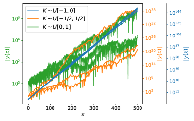
Figure 1: Absolute values of sample realizations of the Jacobi field for different distributions of $K$. The colors correspond to different distributions of $K$. The absolute values of three sample realizations are shown for each distribution. Note the logarithmic scale for the $y$ axes and that each distribution is shown with a separate $y$ axis (the colors of the axes correspond to the colors of the plots). Separate peaks downwards correspond to moments when the Jacobi field changes sign and the absolute value of the Jacobi field approaches zero.

III Invariant measure and the Lyapunov exponent

The mathematical theory on a product of random matrices developed by Furstenberg and Kesten in [13, 14] allows reduction of the Lyapunov exponent from the limit expression (2) to the integration over a particular invariant measure (also known as the stationary distribution). In a simplified notation proposed in [15], it was shown that the sequence of the matrix exponentials $\hat{B}_{i}$ generates an ergodic Markovian chain on the unit sphere $S^{1}$ with identified diametrically opposite points. The ergodicity ensures that any initial distribution on this space converges to the unique stationary distribution (invariant measure).

In [9] it was proposed to obtain the transition density $p(\varphi,\psi)$ of the Markovian chain numerically and then to obtain the solution $\pi(\psi)$ of the stationary distribution equation

$$\pi(\psi)=\int\pi(\varphi)p(\varphi,\psi){\rm d}\varphi\,.$$ (8)

Here $\varphi$ and $\psi$ are in $(-\pi/2,\pi/2]$ and specify the coordinates on the the unit sphere $S^{1}$ with identified diametrically opposite points.

To derive the transition density, one can demonstrate that the variables $\varphi$ and $\psi$ are related by equation

$$\tan\psi=\frac{\tan\varphi-\xi\tan\sqrt{k}}{1+\tan\varphi\tan\sqrt{k}/\sqrt{k}}\,,$$ (9)

where $k=K\Delta^{2}$. Thus, given a distribution of $K$ one can compute the transition density $p(\varphi,\psi)$.

In general, the transition density can not be expressed analytically and should be found numerically. In fact, however, the numerical approach becomes tricky due to various irregularities of the Eq. (9). We skip the technical details of this process, and present in Fig. 2 the final numerical results for the stationary distribution.

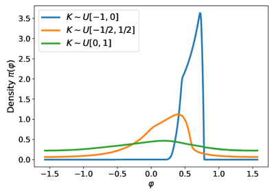
Figure 2: Stationary distribution $\pi(\varphi)$ for various distributions of $K$.

Given the stationary distribution $\pi(\varphi)$ and the distribution $p(K)$ of the curvature parameter, we compute the Lyapunov exponent by numerical approximation of the integral

$$\lambda=\int\log\|{\bf w}{B(K)}\|\pi(\varphi)p(K){\rm d}\varphi{\rm d}K\,,$$ (10)

where ${\bf w}$ is the unit vector $(\cos\varphi,\sin\varphi)$.

In Table 1 we summarize the Lyapunov exponents obtained for uniform distributions of $K$ given that $\Delta=1$. In agreement with Fig. 1 we observe in all cases a positive mean growth rate (the Lyapunov exponent) of the Jacobi field. For positive $K$ this is the manifestation of the resonance of oscillating solutions, while for negative and alternating $K$ this indicates that the exponential growth on the intervals, where $K$ is negative, gives the main contribution to the mean growth rate. Quantitatively, we observe that the growth rate due to resonance is an order of magnitude weaker compared to the alternative scenarios.

$K$	$\lambda$
$U[-1,0]$	0.693
$U[-1/2,1/2]$	0.133
$U[0,1]$	0.018

Table 1: Lyapunov exponents of the Jacobi field for various distributions of $K$.

IV Growth rate of the mean field

The positive values of the Lyapunov exponent imply that the absolute values of individual realizations of the Jacobi field are expected to grow exponentially. At the same time, the mean value of the Jacobi field can be vanishing as we demonstrate below.

Consider the averaging of Eq. (6):

$$\langle{\bf z}\rangle(n\Delta)={\bf z}_{0}\langle\hat{B}\rangle^{n}\,.$$ (11)

This shows that the mean field $\langle{\bf z}\rangle$ grows as the leading eigenvalue of the matrix $\langle\hat{B}\rangle$. More precisely, the growth rate $\gamma$ of the mean field $\langle{\bf z}\rangle$ is obtained as

$$\gamma=\frac{1}{2\Delta}\ln|\lambda_{(1)}|\,,$$ (12)

where $\lambda_{(1)}$ is the leading eigenvalue of the matrix $\langle\hat{B}\rangle$. Note that the growth rate $\gamma$ of the mean Jacobi field should not be confused with the growth rate $\gamma_{1}$ defined in (3). The difference is that $\gamma_{1}$ refers to the growth of the mean absolute value of the Jacobi field, while $\gamma$ refers to the growth of the absolute value of the mean Jacobi field.

For small $\Delta$ the matrix $\langle\hat{B}\rangle$ and then $\lambda_{(1)}$ and $\gamma$ can be approximated in terms of the first several statistical moments of the random variable $K$, i.e. in terms of $\mu=\langle K\rangle$ and $\sigma^{2}=varK$. We consider the cases when $K$ is distributed (1) in the negative domain, (2) in the domain symmetric with respect to zero, and (3) in the positive domain.

The first case ($K$ is negative) yields

$$\gamma=\frac{1}{2}\sqrt{-\mu}+\frac{1}{24}\frac{\sigma^{2}}{\sqrt{-\mu}}\Delta^{2}+O(\Delta^{3})\,.$$ (13)

Note that $\gamma$ does not vanish for $\Delta\to 0$ but tends to some positive value. We will address this fact in the next section.

For the symmetric-distributed $K$ we obtain

$$\gamma=\frac{\sqrt{6}}{12}\sigma\Delta+O(\Delta^{3})\,,$$ (14)

and $\gamma$ vanishes for $\Delta\to 0$.

Finally, for the positive $K$ we obtain

$$\gamma=-\frac{1}{48}\sigma^{2}\Delta^{3}+O(\Delta^{4})\,.$$ (15)

Here we note that for small $\Delta$ the growth rate $\gamma$ becomes negative.

For illustration, consider uniform distributions for the parameter $K$, similar to those we considered for numerical estimation of the Lyapunov exponent. In all cases $\sigma^{2}=1/12$, but $\mu=-1/2$ for $K\sim U[-1,0]$, $\mu=0$ for $K\sim U[-1/2,1/2]$, and $\mu=1/2$ for $K\sim U[0,1]$. Fig. 3 shows the analytical approximations of $\gamma$ in comparison with its numerical estimates. For the numerical estimates we simulated $10^{6}$ realization of random matrices $\hat{B}$, computed the leading eigenvalue of the sample averaged matrix, and then derived $\gamma$. We observe that the analytical approximations (13)–(15) are in agreement with the numerical simulation at least for small $\Delta$. Of course, one can improve the agreement by adding terms of the higher orders in (13)–(15), however, these terms will include higher statistical moments of the random variable $K$.

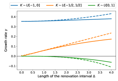
Figure 3: Growth rate $\gamma$ of the mean Jacobi field for different distributions of $K$. Solid lines show numerical estimates, dashed lines show analytical approximations.

V Second-order statistical moment

Following [10], the growth rate of $\langle\|{\bf z}\|^{2}\rangle$ can be associated with the growth rate of matrix product. To show this, introduce a vector ${\bf q}$ of pairwise products of the components of vector ${\bf z}$, i.e.

$${\bf q}=(z_{1}z_{1},z_{1}z_{2},z_{2}z_{1},z_{2}z_{2})\,.$$ (16)

Taking the derivative of ${\bf q}$ and using the Jacobi equation in the form of (5), one obtains the equation

$${\bf q}^{\prime}={\bf q}A\,.$$ (17)

Similar to (6), the solution $q(n\Delta)$ is represented by the product of independent and identically distributed matrix exponentials $\exp(A_{i}\Delta)$. It follows that

$$\langle{\bf q}\rangle(n\Delta)=q_{0}\langle\exp(A\Delta)\rangle^{n}\,$$ (18)

and the growth rate of the mean vector $\langle{\bf q}\rangle$ is given by the leading eigenvalue of the mean matrix exponential $\langle\exp(A\Delta)\rangle$. But the first component of the vector $\langle{\bf q}\rangle$ is $\langle z_{1}^{2}\rangle=\langle y^{2}\rangle$ and thus the leading eigenvalue also defines the growth rate of $\langle y^{2}\rangle$.

The matrix exponential $\hat{A}=\exp(A\Delta)$ can be found explicitly (see [10]) and reads

$$\hat{A}=\begin{pmatrix}\cos^{2}\sqrt{k}&\frac{\sin 2\sqrt{k}}{2\sqrt{k}}&\frac{\sin 2\sqrt{k}}{2\sqrt{k}}&\frac{\sin^{2}\sqrt{k}}{k}\\ \frac{-\sqrt{k}\sin 2\sqrt{k}}{2}&\cos^{2}\sqrt{k}&-\sin^{2}\sqrt{k}&\frac{\sin 2\sqrt{k}}{2\sqrt{k}}\\ \frac{-\sqrt{k}\sin 2\sqrt{k}}{2}&-\sin^{2}\sqrt{k}&\cos^{2}\sqrt{k}&\frac{\sin 2\sqrt{k}}{2\sqrt{k}}\\ k\sin^{2}\sqrt{k}&\frac{-\sqrt{k}\sin 2\sqrt{k}}{2}&\frac{-\sqrt{k}\sin 2\sqrt{k}}{2}&\cos^{2}\sqrt{k}\end{pmatrix}\,,$$ (19)

where $k=K\Delta^{2}$ similar to (7). For small $\Delta$ the mean matrix exponential $\langle\hat{A}\rangle$ and its leading eigenvalue $\lambda_{(1)}$ can be approximated in terms of the statistical moments of the random variable $K$. Then taking into account the relation between the leading eigenvalue $\lambda_{(1)}$ and the growth rate $\gamma_{2}$

$$\gamma_{2}=\frac{1}{4\Delta}\ln|\lambda_{(1)}|\,,$$ (20)

we obtain the following estimates.

For $K$ distributed in the negative domain (note that $\mu<0$ in this case) we obtain

$$\gamma_{2}=\frac{1}{2}\sqrt{-\mu}-\frac{1}{16}\frac{\sigma^{2}}{\mu}\Delta+O(\Delta^{2})\,.$$ (21)

For the symmetric-distributed $K$:

$$\gamma_{2}=\frac{1}{4}(2\sigma^{2})^{\frac{1}{3}}\Delta^{\frac{1}{3}}+O(\Delta)\,.$$ (22)

For $K$ distributed in the positive domain:

$$\gamma_{2}=\frac{1}{8}\frac{\sigma^{2}}{\mu}\Delta+O(\Delta^{2})\,.$$ (23)

It can be noted, that for $K$ distributed in the negative domain $\gamma_{2}\not\to 0$ as $\Delta\to 0$. Our interpretation of the fact is as follows. The scalings (21) and (13) refer to the model where the solution grows in each renovation interval. For the vanishing $\Delta$ the noise effects vanish and we obtain the positive growth rate associated with the mean curvature, i.e. a non-random contribution to the instability. The scaling (23) deals with the instability intrinsically related to the noise in the curvature. When $\Delta\to 0$ the noise contribution vanishes, and the growth rate also vanishes. It is also interesting to note that while (15) yields that the mean of the oscillating field vanishes, the mean energy grows exponentially according to (23).

Fig. 4 illustrates the estimates of the growth rate $\gamma_{2}$ obtained numerically and following (21)–(23) for three cases of uniform distribution of $K$. The numerical approach is similar to those used in Fig. 3. Again, we observe that the analytical approximations are in agreement with the numerical simulations for small $\Delta$. The agreement for larger $\Delta$ can be improved by adding terms of the higher orders in series (21)–(23), but they will include higher statistical moments of the random variable $K$.

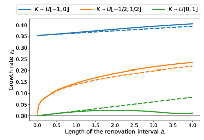
Figure 4: Growth rate $\gamma_{2}$ for different distributions of $K$. Solid lines show numerical estimates, dashed lines show analytical results

VI Conclusions and discussion

We obtained that self-excitation with random positive growth rates is more efficient than the competition of self-excitation and oscillations, which, in turn, is more efficient than the cumulative resonance effect of random oscillations. This message looks quite natural, but the fact that random oscillations lead to instability is not so obvious. The latter statement follows from the general mathematical theory [15], but the quantitative relationship between the three above-mentioned growth rates remained untouched by previous studies.

Consider the above results in the light of the dynamo problem. There are two realizations of general dynamo process that are believed to be relevant for, say, solar physics. First, there is a conventional solar dynamo based on a joint action of differential rotation and mirror asymmetry of solar convection. The both drivers taken together close the chain of self-excitation and provide the growing magnetic field. The growth is noisy, however, it becomes more and more regular if the noise contribution disappears ($\Delta$ becomes small in comparison to the dynamo time scale). Note that in this paper we considered the limiting case $\Delta\to 0$ and the noise amplitude remained fixed. Of course, one can also consider the case $\Delta\to 0$, while the noise amplitude becomes larger as an appropriate power of $1/\Delta$ to get a non-vanishing growth rate (a short-correlated model).

Another type of dynamo mechanism, possibly related to the solar dynamo, is the so-called small-scale dynamo. This mechanism contains no specific driving forces. It is based only on random velocity fluctuations and can be compared to the third case in our analysis, i.e., random positive $K$. If the noisy contribution disappears, the growth rate becomes negligibly small and the generated magnetic field remains noisy.

Of course, the above messages can be derived from extensive direct numerical MHD modeling, but it is useful to know that the results obtained from simulations reflect general properties of dynamical systems and can be supported by examples available for analytical analysis.

Our analysis is performed within the simple framework proposed in [5], but as far as we know, the problem is not specific, and analysis of more complicated systems requiring a more bulky algebra is not expected to lead to more dramatic results (see, e.g., [16]). It is also an open question how the more complicated forms of the random process can influence the form and stability of the amplification of the mean field and mean energy. We hope to address these questions in future research.