general iterative approximation to differential equations.

Abstract.

This article provides a general iterative approximation to partial differential equations, and thus establish existence of smooth solution. The heart of the method is to contract (or expand) the boundary conditions uniformly in the domain, then using local and global correspondence to transform discrete step function to successive integration on the domain. Numerical scheme is discussed and tested for Navier-Stokes equation.

1. introduction

Let $\Omega\subset\mathbb{R}^{n}$ be a domian with smooth boundary $\partial\Omega$, let $P={P_{1},P_{2},\ldots,P_{k}}$ be a partition of $\mathbb{R}^{n}$. Denote by $u_{i}:\Omega\to P_{i}$ unknown vector functions defined on the chart $x$, denote $y_{i}$ a one dimensional parameter of the chart $y$. Let $\phi$ be a coordinate transform from the chart $y$ to $x$ so that

$$span_{j\neq i}\frac{\partial\phi}{\partial y_{j}}(\partial\Omega)=T\partial\Omega_{i}\quad span_{j=1}^{n}\frac{\partial\phi}{\partial y_{j}}(\Omega)=T\Omega\quad\cup_{i=1}^{n}T\partial\Omega_{i}=T\partial\Omega,$$

where $\partial\Omega_{i}$ has dimension $dim(P_{i})-1$. Consider a system of differential equations that can be written in the form:

(1.1) $$\frac{\partial u_{i}(\phi y)}{\partial y_{i}}= F_{i}(u,y)\quad u_{i}(\partial\Omega_{i})=w_{0}\quad i=1,\ldots,l$$

$$\frac{\partial u_{j}(\phi y)}{\partial y_{j}}= F_{j}(u,y)\quad u_{j}(\partial\Omega_{j})=W_{j}(u_{i},y)\quad j=l+1,\ldots,k$$

where the functionals $F_{i}$, $F_{j}$ and $W_{j}$ are completely determined, $w_{0}$ represents initial and boundary conditions. Equation (1.1) covers many mathematical physical equations that appear in nature and industry, such as hydrodynamic equations, wave equations and statistical equations. For example, the imcompressible Navier-Stokes equation can be written in the form of equation (1.1):

$$\frac{\partial u}{\partial t} =-u\cdot\nabla u+\mu\Delta u+f-grad\,p\quad u(t=t_{0})=u_{0}$$

$$\frac{\partial p}{\partial y_{j}} =q\quad p(\partial\Omega)=p_{0}$$

$$\frac{\partial q}{\partial y_{j}} =-\frac{\partial q}{\partial y_{k}}-g(y)\,q+div\,(-u\cdot\nabla u+\mu\Delta u+f)\quad q(\partial\Omega)=q_{0}(u)\quad k\neq j$$

The problem of determining the general conditions for existence of solution to equation (1.1) is a long standing open problem in mathematics [Fe2006]. Besides theoretical interests, an iterative algorithm that approximate solution to such equations accurately and efficiently has potentially a wide range of applications.

Current progress on this problem is too vast to survey thoroughly, to name a few aspects: weak solutions, finite element methods and various strong solutions in special cases. Examples of non-uniqueness and finite time blow-up can be found in literature [BuDrShVi2022]. The goal of this article is to prove that the conditions specified in equation (1.1) are necessary and sufficient for the existence of smooth solution, by constructing an iterative approximation that converge to it.

Theorem 1.

The following sequences converge to the solution of equation (1.1) as $\lim m,p\to\infty$:

(1.2) $$U(i,0)= w_{0}\quad$$

$$U(i,m+1)= U(i,0)+$$

$$+\lim_{p\to\infty}\int_{y_{i}\,proj\,\partial\Omega}^{y_{i}} F_{i}(U(1,m),\ldots,U(l,m),U(l+1,m,p),\ldots,U(k,m,p),y)\,dy_{i}$$

$$\mathrm{for}\>i=1,\ldots,l.\>\mathrm{And}$$

$$U(j,m,0)= W_{j}(U(1,m),\ldots,U(l,m),y)\quad$$

$$U(j,m,p+1)= U(j,m,0)+$$

$$+\int_{y_{j}\,proj\,\partial\Omega}^{y_{j}} F_{j}(U(1,m),\ldots,U(l,m),U(l+1,m,p),\ldots,U(k,m,p),y)\,dy_{j}$$

for j=l+1,…,k.

Different partition index $i<k$ corresponds to dependent sequences, i.e. each sequence takes limit in each step of another sequence to converge to the solution $u$. Notice that setting $U(i,m+1)=U(i,m)$ in the inductive expression (1.2) automatically implies $U(i,m)$ is a solution to equation (1.1), the problem reduce to proving the convergence of the sequences (1.2).

A corresponding step method for numerical computations is also introduced. The step method provides a more efficient alternative to finite elements, since each step takes only linear operations.

2. convergence and error estimate

Notations for $F,\,W,\,y$ and others follow previous section. Let $L$ be a Lipschitz constant that bounds the functionals $W(u,y)$, $F(u,y)$ and boundary conditions $w_{0}$. Recall that $\frac{\partial\phi}{\partial y_{i}}$ are transvesal to the boundary $\partial\Omega$, so that $\frac{\partial u}{\partial y_{j}}(\partial\Omega)\quad j\neq i$ is completely determined. Let $T\geq|y_{i}-y_{i}\,proj\,\partial\Omega|$ be an integration bound for all $i$. The convergence for the inductive sequences (1.2) may now be proved.

proof of theorem 1.

For simplicity denote $f(m)=|U(m+1)-U(m)|$ the maximum of $|U(i,m+1)-U(i,m)|$ for all partition index $i=1,\ldots,k$. Substitute the inductive expression (1.2) into $f(m)$

$$f(m)= |\int^{y_{i}}_{y_{i}\,proj\,\partial\Omega}(F(U(m),y)-F(U(m-1),y))\,dy_{i}|$$

$$\leq \int^{y_{i}}_{y_{i}\,proj\,\partial\Omega}L|U(m)-U(m-1)|\,dy_{i}$$

$$\leq \frac{1}{2}L\,T\,f(m-1)$$

By induction on $m$, a bound for $f(m)$ is obtained

$$f(m)\leq\frac{1}{m!}\,L^{m}\int^{y_{i}}_{y_{i}\,proj\,\partial\Omega}|F(U(0))|\,y_{i}^{m}\,dy_{i}\leq\frac{1}{(m+1)!}\,L^{m+1}\,T^{m+1}$$

Since

$$\lim_{m\to\infty}U(i,m)\leq U(0)+\sum_{m=0}^{\infty}f(m)\leq w_{0}+e^{L\,T},$$

I now conclude that $U(i,m)$ converge uniformly as $m\to\infty$, by Weierstrass M test. The same reasoning hold for $U(j,m,p)$. ∎

Denote the error term $R(m^{\prime})=\sum^{\infty}_{m=m^{\prime}+1}f(m)$ for order $m^{\prime}$, which is bounded by the Lagrange remainder term:

(2.1) $$R(m^{\prime})\leq\sum^{\infty}_{m=m^{\prime}+1}\frac{1}{m!}(L\,T)^{m}\leq\frac{1}{(m^{\prime}+1)!}\,(L\,T)^{m^{\prime}+1}\,e^{L\,T}\,.$$

Notice that the error may increase initially when $L\,T$ is large, but eventually converge.

3. step method

To obatin numerical solutions efficiently, there is a corresponding step method to the iterative approximation (1.2), which sometimes takes less computational resource than successive integration. The basic idea is that when the step size $dy$ is small enough, the following may be equalized:

$$u(y_{0}+dy)=u(y_{0})+\int_{y_{0}}^{y_{0}+dy}F(u,y)\,dy\approx u(y_{0})+F(u(y_{0}),y_{0})\,dy.$$

Consider a simplified differential system of equation (1.1), $\frac{\partial u}{\partial y}=F(u,y)$. Suppose the integration interval is $T$, and the total step number is $N=\frac{T}{dy}$. Denote $u(y_{0}+m\,dy)$ by $U(m)$, the iterative expression for each step is obtained:

(3.1) $$U(0) =u(y_{0})$$

$$U(m+1) =U(m)+F(U(m),m)\,dy$$

with $U(N)$ the numerical solution sought. To prove convergence, it suffice to prove that the step method (3.1) is actually equivalent to the iterative approximation (1.2) when $\lim dy\to 0$. Observe that

$$U(m+1) =U(m)+F(U(m),m)\,dy$$

$$=U(m-1)+(F(U(m-1),m-1)+F(U(m),m))\,dy.$$

By induction on $m$

$$U(m+1)=U(0)+\sum^{m}_{m^{\prime}=0}F(U(m^{\prime}),m^{\prime})\,dy.$$

Then take $dy\to 0$

$$\lim_{dy\to 0}U(m+1)=U(0)+\int_{y_{0}}^{y}F(U(m),y)\,dy\quad,$$

which has exactly the same form as the iterative approximation (1.2). I may conclude that the step method (3.1) converges to the iterative approximation (1.2) as $dy\to 0$ by this local and global correspondence.

error bound

Let $L$ be the Lipschitz constant that bounds $F(u)$ as before. In case of uniform step size $dy$, denote by $\overline{u}(m)$ the solution obtained by step method at $m$-th step. Denote by $u(m)$ the actual solution. Denote by $R(m)=|\overline{u}(m)-u(m)|$ the error term. Then

$$R(m+1) =|\overline{u}(m)+F(\overline{u}(m))\,dy-u(m)-\int_{m}^{m+1}F(u(y))\,dy|$$

$$\leq R(m)+|F(\overline{u}(m))-F(u(m+1))|\,dy$$

$$\leq R(m)+|F(\overline{u}(m))-F(u(m))|\,dy+|F(u(m))-F(u(m+1))|\,dy$$

$$\leq R(m)+L\,R(m)\,dy+L^{2}\,dy.$$

Set $R(0)=0$, by induction on $m$

$$R(N)\leq(1+L\,dy)^{N}\,R(0)+L^{2}\,dy\sum^{N-1}_{m^{\prime}=0}(1+L\,dy)^{m^{\prime}}=L^{2}\,dy\sum^{N-1}_{m^{\prime}=0}(1+L\,dy)^{m^{\prime}}.$$

This is the error bound for the step method at $N$-th step. The error increases further away from the boundary.

4. example: Navier-Stokes equations

To demonstrate intuitively the accuracy of the step method (3.1), consider the imcompressible Navier-Stokes equations:

(4.1) $$\frac{\partial u}{\partial t} =-u\cdot\nabla u-grad\,p+\Delta u$$

$$\Delta p =div(-u\cdot\nabla u+\Delta u)\,,$$

where the Poisson equation for $p$ is obtained by taking the derivative of incompressible condition $div(u_{t})=0$ and substituted into the first equation. Finding numerical solution to Navier-Stokes equation is then equivalent to iterate step function (3.1) for Poisson equation of $p$ at each step of $u$. The step function for $u$ is

$$u(i+1)=u(i)+(-u(i)\cdot\nabla u(i)-grad\,p(i)+\Delta u(i))\,dt.$$

To compare intuitively the accuracy of the step method, consider for example the Taylor-Green vortex, an analytic solution to Navier-Stokes equation

$$u =(\sin(x)\cos(y)\,e^{-2t},-\cos(x)\sin(y)\,e^{-2t})$$

$$p =\frac{1}{4}\cos(2x)\,\cos(2y)\,e^{-4t}.$$

Assuming the solution to Poisson equation of $p$ is known for each $u$, the step function for $u$ may be iterated from $t=0$, see figure 1.

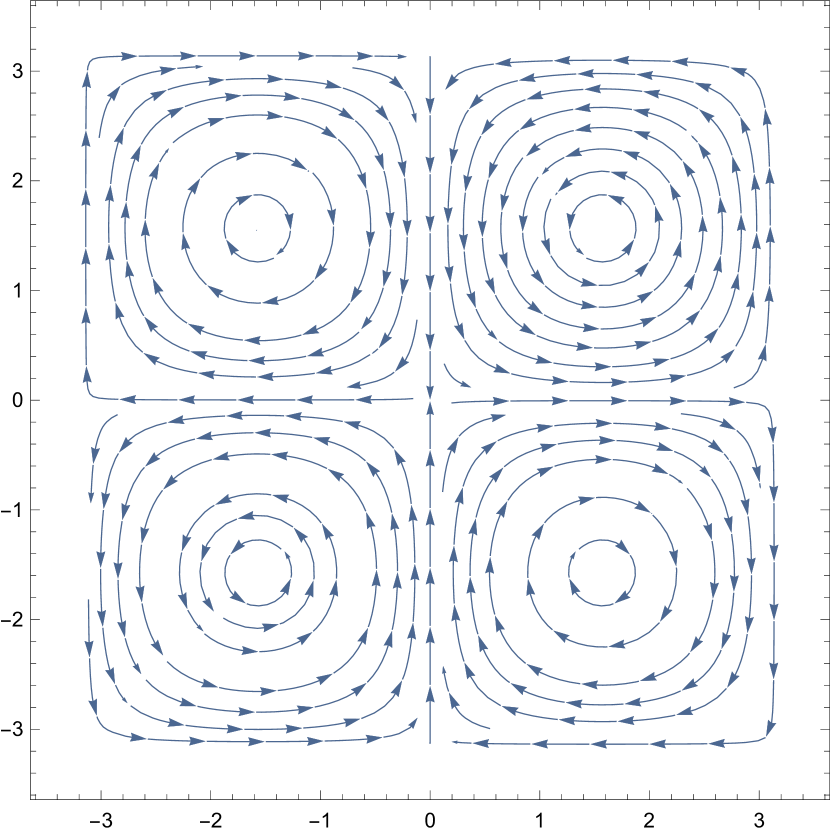
(a) Analytic solution at time 1 exhibits saddle connections.

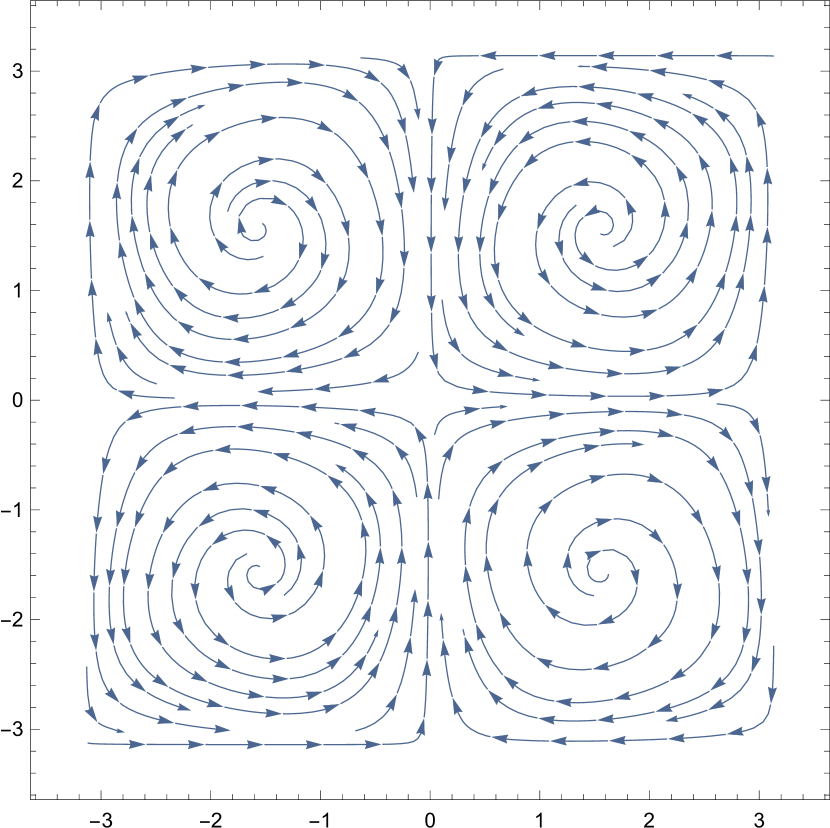
(b) Step function at time 1 with step size 0.25 .

Figure 1. Taylor-Green vortex.

The central difference between solving ODEs’ and PDEs’ with step method is that PDEs’ take derivatives at each step, while ODEs’ are purely numerical. One way to optimize this algorithm is to find the closed-form solution to the step function. This is achieved by treating the differential operators as linear coefficients, and then solve the corresponding linear difference equation. Though the specific computation time for a given goal depends on the form of the equation, the shape of boundary and boundary conditions, substituting derivatives into closed form significantly reduces computation time.

Consider the step function for Poisson equation of $p$ with circular boundary conditions, denote $f(j)=div(-u(i)\cdot\nabla u(i)+\Delta u(i))$ the right hand side of poisson equation at $j$-th step away from boundary

$$p(j+1) =p(j)+q(j)\,dr$$

$$q(j+1) =q(j)+(f(j)+\frac{q(j)}{r(j)}-\frac{1}{r(j)^{2}}\frac{\partial^{2}p(j)}{\partial\theta^{2}})\,dr$$

where $q=\frac{\partial p}{\partial r}$. The right hand side of $q$ is just laplacian in polar coordinates, where the differential operators satisfy $\frac{\partial}{\partial r}=\frac{-x}{\sqrt{x^{2}+y^{2}}}\frac{\partial}{\partial x}+\frac{-y}{\sqrt{x^{2}+y^{2}}}\frac{\partial}{\partial y}$ and $\frac{\partial}{\partial\theta}=-y\frac{\partial}{\partial x}+x\frac{\partial}{\partial y}$.

Another optimization approach is to consider stable solution of the corresponding linear system, which will not be addressed in this article. The step method introduced above adapts to systems of arbitrary dimensions and order, should enough boundary conditions be supplmented.

5. conclusions

The iterative approximation described in this article estabishes the existence of smooth solution to a wide class of, if not all, partial differential equations. Additionaly, the corresponding step method provides a potentially more efficient numerical scheme for solving equations than existing methods, if the algorithm is properly optimized. No doubt the method opens up new paths to the understanding of turbulence bifurcations phenomena.

One of the key element of the method is choosing the appropriate differentiation transformation, as described at the beginning of this article, so the entire boundary continuously contract to a single point. The local and global correspondences connects discrete steps of this contraction to successive integration on the entire domain.