Data-driven estimation of transfer integrals in undoped cuprates

Abstract

Undoped cuprates are an abundant class of magnetic insulators, in which the synergy of rich chemistry and sizable quantum fluctuations leads to a variety of magnetic behaviors. Understanding the magnetism of these materials is impossible without the knowledge of the underlying spin model. The typically dominant antiferromagnetic superexchanges can be accurately estimated from the respective electronic transfer integrals. Density functional theory calculations mapped onto an effective one-orbital model in the Wannier basis are an accurate, albeit computationally cumbersome method to estimate such transfer integrals in cuprates. We demonstrate that instead an Artificial Neural Network (ANN), trained on the results of high-throughput calculations, can predict the transfer integrals using the crystal structure as the only input. Descriptors of the ANN model encode the spatial configuration and the chemical composition of the local crystalline environment. A virtual toolbox employing our model can be readily employed to determine leading superexchange paths as well as for rapidly assessing the relevant spin model in yet unknown cuprates.

1 Introduction

The data-driven approach accompanied by modern machine-learning (ML) techniques becomes an increasingly important tool of scientific investigations across many domains of physics. From quantum to fluid mechanics tsubaki.prl.20 ; brunton.annurev-fluid.20 learning from data facilitates descriptions of complex phenomena for which analytical approaches are prohibitively challenging. The adoption of ML in solid-state physics and material science is particularly appealing: the sheer amount of collected experimental and computed records propels the community to design data-driven frameworks for prediction of materials properties scmidt.npj.compmat.19 ; xie.prl.20 .

The application of ML for problems of solid-state physics is not straightforward. One of the key challenges is to represent periodic (crystalline) or finite (molecule, local crystal environment, etc.) atomic systems as descriptors – data structures amenable to ML methods. Such descriptors must be invariant with respect to the choice of the unit cell (crystals) or to global rotations in a finite system. Several classes of descriptors have been developed for material properties prediction: Coulomb matrix rupp.prl.12 , partial radial distribution function (PRDF) schtt.prb.2014 , smooth overlap of atomic positions (SOAP) bartok.prb.2013 , diffraction fingerprint (DF) ziletti.natcomm.2018 and three-dimensional (3D) Zernike descriptor (3DZRD) venkatraman.joc.09 . The latter were designed for the characterization of 3D shapes novotni2003 ; novotni.shape.04 and successfully employed for comparison of molecules sael.prot.2008 ; mak.jmgm.2008 ; sael2008 . These descriptors are invariant with respect to the number of chemical species in the dataset, they store detailed information about the spatial arrangement, and do not require additional simulation software. These features as well as the compact size of the resulting data structures make 3DZRD ideally suited for a description of diverse, dissimilar crystalline environments.

Another key challenge is the construction of descriptors that represent material properties. For instance, it is widely accepted that electronic, magnetic, and topological properties of bulk materials are rooted – in a highly nontrivial way — in their electronic structure. However, using the complete band structure of a material as a universal descriptor is not possible for a number of reasons: different number of bands, non-universal discretization of the Brillouin zone, huge dimensionality etc. A more practical approach is to restrict the description to the states relevant for the physical quantity of interest. Naturally, this is possible only for a certain class of materials and only for specific physical property.

Following this idea, we apply a data-driven approach to assess spin models in undoped cuprates – stoichiometric inorganic materials containing divalent copper and oxygen atoms. In contrast to their doped counterparts – the high-temperature cuprate superconductors Plakida2010htc – undoped cuprates are magnetic insulators with the $3d^{9}$ electronic configuration of Cu²⁺. The sizable Jahn-Teller distortion lifts the orbital degeneracy, giving rise to half filling and localized $S$=$\frac{1}{2}$ spins. Owing to the plethora of structure types and the quantum limit assured by $S$=$\frac{1}{2}$, undoped cuprates exhibit a variety of magnetic behaviors sahadasgupta2021 , from simple quantum dimers and spin chains – to exotic collective behaviors such as the spin-liquid regime in herbertsmithtite $\gamma$-Cu₃Zn(OH)₆Cl₂ helton07 , Bose-Einstein condensation of magnons in Han purple BaCuSi₂O₆ jaime04 , or bound magnon states in volborthite Cu₃V₂O₇(OH)${}_{2}\cdot 2$H₂O kohama19 .

Understanding the magnetic properties of cuprates requires the knowledge of the underlying spin model. While exchange anisotropies are generally present and can alter the magnetic properties, the backbone of spin models are isotropic interactions, and the relevant Heisenberg Hamiltonian is the following sum:

$$\mathcal{H}=\frac{1}{2}\sum_{ij}J_{ij}\left(\mathbf{S}_{i}\cdot\mathbf{S}_{j}\right),$$ (1)

where $\mathbf{S}_{i}$ and $\mathbf{S}_{j}$ are spin operators on sites $i$ and $j$. The set of relevant magnetic exchange integrals $\{J_{ij}\}$ determines the spin model. It is important to note that each individual $J_{ij}$ term is a sum of antiferromagnetic ($J^{\text{AF}}_{ij}<0$) and ferromagnetic ($J^{\text{FM}}_{ij}<0$) contributions that are driven by competing processes Goodenough_Magnetism . Commonly, $J^{\text{AF}}_{ij}\gg\lvert{}J^{\text{FM}}_{ij}\rvert$, with the exception of short-range exchanges for which the ferromagnetic contribution can become dominant.

The antiferromagnetic contribution is a textbook example of the superexchange mechanism and can be derived via second-order perturbation theory of the Hubbard model in the strong-coupling limit at half-filling as $J^{\textsc{AF}}_{ij}=4t_{ij}^{2}/U_{\text{eff}}$ hubbard63 ; anderson59 ; auerbach2000 . Here, $U_{\text{eff}}$ is the Coulomb repulsion within an effective molecularlike orbital, which in most cuprates is dominated by $3d_{x^{2}-y^{2}}$ orbital of Cu and $\sigma$-bonded $2p$ orbitals of O. There is empirical evidence that $U_{\text{eff}}$ from the range 4–5 eV gives a proper description of the magnetism of cuprates belik2004 ; johannes2006 ; janson2009 . Hence, the knowledge of transfer integrals $t_{ij}$ paves the way to a quantitative assessment of the spin model in the majority of cuprate materials. Yet, extracting $t_{ij}$ directly from the structural information is essentially impossible; instead, it requires first-principles calculations followed by an additional modeling.

To overcome this challenge, we propose a data-driven approach for prediction of transfer integrals in cuprates, which requires the crystal structure as the only input. Our approach is based on the local crystal environment description utilizing 3DZRD. The local crystal environment descriptor is used as input for the ML model which is trained on the results of high-throughput density-functional-theory (DFT) calculations for hundreds of cuprate materials. DFT calculation for each material is followed by automatized Wannierization and a manual quality control. The trained model is wrapped into a freely accessible web application that can be used for a quick estimation of relevant transfer paths in new cuprate materials.

The paper is organized as follows: Section 2 describes the high-throughput DFT calculations and the dataset of transfer integrals. Section 3 details the descriptor for the Cu..Cu bonds. In Section 4 we compare three different ML approaches for predicting transfer integrals and estimate the accuracy by a cross-validation procedure (CV). In the last section, we discuss the performance of our ML model for different classes of cuprates. In particular, for the parent (undoped) compounds of high-temperature superconducting cuprates we show that the ANN model quantitatively captures the ratio between nearest and next-nearest-neighbor transfer integrals.

2 Dataset generation

We start with the description of the high-throughput DFT calculations employed for the generation of the dataset of transfer integrals. The list of materials contains 672 unique structures of undoped cuprates. The structures were filtered out from the 10 710 cuprate structures stored in the Inorganic Crystal Structure Database (ICSD) bergerhoff.crystallographic.1987 . For this screening, the following criteria were consecutively applied: (i) the presence of Cu²⁺ ions, (ii) electroneutrality (zero total charge), (iii) absence of sites with fractional occupancies, (iv) the minimal inter-atomic distance of 0.5 Å, and (v) the absence of other magnetic atoms beyond Cu suppl . The latter criterion is necessary to filter out compounds with multiple magnetic atoms, where the presence of additional bands in the relevant energy range may render the effective one-orbital model inapplicable and its results misleading. For the analysis of the crystal structures we used the pymatgen library Ong2013pymatgen for Python.

For each structure, we performed DFT calculations to construct Wannier Hamiltonians and subsequently determined the transfer integrals. All DFT calculations were performed using the generalized gradient approximation (GGA) perdew.prl.1996 with the full potential code FPLO of version 18.00-52 koepernik.prb.1999 . The computational workflow comprised several steps. First, scalar-relativistic nonmagnetic DFT calculations were carried out and the Hellmann-Feynman forces were calculated. Second, for hydrogen-containing compounds whose calculated forces exceeded the threshold of 0.1 eV/Å, we optimized the internal coordinates of H atoms within GGA. The rationale behind this step are largely inaccurate H positions as determined by x-ray diffraction (which is by far most common method of structure determination). Since a considerable number of cuprates contain hydrogen, typically as hydroxyl groups or water molecules, inclusion of such partly optimized structures allowed us to considerably extend the data set. All other cuprates whose forces exceeded the threshold 0.1 eV/Å were discarded. Third, we calculated the orbital-resolved density of states (DOS) and band structure. From the orbital-resolved DOS, the energy interval which contains the copper $3d_{x^{2}-y^{2}}$ bands was determined. The energy interval is selected such that the contribution of the magnetic $3d_{x^{2}-y^{2}}$ orbital in the total density of Cu $3d$ states exceeds 5 %. The determined energy window $[\mathscr{E}_{\textsc{min}},\mathscr{E}_{\textsc{max}}]$ was adopted for Wannierization in the next step. Fourth, the Wannier transformation procedure was performed to obtain the effective one-orbital Hamiltonian $H$ in the Wannier basis. We used copper $3d_{x^{2}-y^{2}}$ orbitals as projectors and the interval $[\mathscr{E}_{\textsc{min}},\mathscr{E}_{\textsc{max}}]$ as the energy window to construct the Wannier functions (WF). The latter is necessary to discriminate the target antibonding orbital (crossing the Fermi energy) from its bonding sibling at the bottom of the valence band. The transfer integral between two WF $w_{i}$ and $w_{j}$ placed at copper sites $i$, $j$ is determined as (real) Hamiltonian matrix element $t_{ij}=\langle{}w_{i}\lvert{}H\rvert{}w_{j}\rangle$. The details on the construction of Wannier functions and the construction of the respective tight-binding models are provided in the papers koepernik2021arxiv ; eschrig2009 .

After the calculation pipeline was completed, we obtained a list of transfer integrals $\{t_{ij}\}$ that connected $i$-th and $j$-th copper sites situated at the distance $r_{ij}$ from each other for all valid structures suppl . For construction of the dataset we select transfer integrals larger than 5 meV with Cu..Cu spacing less than 8 Å. The distribution of calculated transfer integrals $t_{ij}$ among Cu..Cu distances is shown in Fig. 2. The crystal chemistry of cuprates sets a natural lower limit for the bond lengths; accordingly, there is no transfer integral with the distance less than 2.4 Å in the dataset. Remarkably, for the vast majority of transfer integrals, the absolute values are below 0.2 eV. This natural imbalance of the dataset will inevitably affect the performance of predictions.

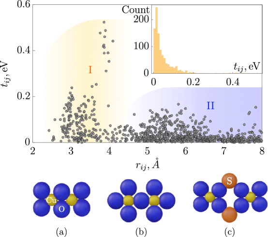
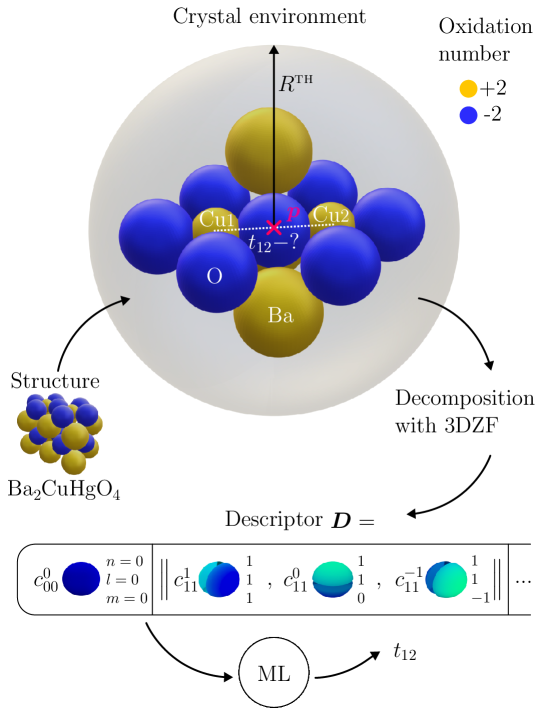
Figure 1: (Color online) Transfer integrals obtained from the DFT calculations as a function of the Cu..Cu distance. Region I harbors transfer integrals between edge-sharing (a) and corner-sharing (b) CuO₄ plaquettes, while region II is dominated by transfer integrals between CuO₄ plaquettes that do not share oxygen atoms (c). The inset shows the distribution of the computed transfer integrals.

Figure 2: (Color online) Schematics of the workflow: selection of the local crystal environment from the cuprate crystal structure, generation of rotationally invariant descriptor $\vec{D}$ via decomposition of the local crystal environment function in the truncated basis of 3DZF and prediction of the transfer integral $t_{ij}$ with ML algorithm trained on the dataset from DFT calculations. The illustrating example Ba₂CuHgO₄ (ICSD Identifier 75724) hosts pairs of corner-sharing CuO₄ square-like plaquettes.

3 Crystal Environment Descriptor

To describe the crystal environment, we first determine the midpoint $\vec{p}$ between a given pair of copper atoms and build a sphere with the empirically determined threshold radius $R^{\textsc{th}}=\max(4,r_{ij}/2+0.2)$ Å centered at $\vec{p}$. Next, all atoms in the sphere are enlisted in the crystal environment alongside with nearest neighbors of $i$ and $j$. We consider nearest neighbors as atoms distanced from $i$ or $j$ not farther than 2.5 Å. After the local crystal environment is assembled, we shift the coordinate system origin to the centroid (the point between copper pair) $\vec{p}$ and normalize atoms coordinates by $r_{0}=6$ Å to fit the crystal environment in the unit ball. To construct a robust representation of the local crystal environment we introduce the piecewise function of site positions $\mathcal{I}(\vec{r})$. The function $\mathcal{I}$ equal to the $q$-th atom oxidation number $O_{q}$ in the ball with center at the position of $q$-th atom $\vec{r}_{q}$ and radius $R_{q}$ equals to the ionic radius of the atom

$$\mathcal{I}(\vec{r})=\begin{cases}O_{q}&\|\vec{r}_{q}-\vec{r}\|\leq R_{q},\\ 0&\text{otherwise}.\end{cases}$$ (2)

The normalization factor $r_{0}$ is a sum of the maximal considered Cu-Cu distance $\max\|\vec{r}_{ij}\|=4$ Å and a maximal considered ionic radius $2$ Å. The function $\mathcal{I}(x,y,z)$ describes the spatial configuration and chemical composition of the crystal environment placed in the unit ball with $x^{2}+y^{2}+z^{2}\leq 1$. An example of the local crystal environment defined by (2) is shown in Fig. 2.

We describe the selected crystal environment $\mathcal{I}$ in the form of a finite-dimensional vector. Such representation provides a robust way for numerical operations with crystal environments, e.g. similarity and sorting. To obtain the finite vector representation of the crystal environment we decompose the $\mathcal{I}(x,y,z)$ in the truncated basis of three-dimensional (3D) Zernike functions (3DZF) $Z^{m}_{nl}$ which are defined as follows canterakis96 ; canterakis99 ; novotni.shape.04

$$\begin{split}Z_{nl}^{m}(r,\theta,\phi)&=R_{nl}(r)Y_{lm}(\theta,\phi),\\ R_{nl}(r)&=\sum_{\nu=0}^{(n-l)/2}Q_{l\nu}r^{2\nu+l},\\ Q_{l\nu}&=\dfrac{(-1)^{k+\nu}}{4^{k}}\sqrt{\dfrac{2l+4k+3}{3}}\dfrac{\binom{2k}{k}\binom{k}{\nu}\binom{2(k+l+\nu)+1}{2k}}{\binom{k+l+\nu}{k}},\end{split}$$ (3)

where indices $n$ and $l$ are positive integers which satisfy condition $n\geq l$; $m$ changes from $-l$ to $l$ with constraint $(n-l)$ is even number; $k=(n-l)/2$ and $Y_{lm}(\theta,\phi)$ are spherical harmonics, and $(r,\theta,\phi)$ are spherical coordinates nist.math.handbook . For convenience, we use Cartesian coordinates $(x,y,z)$ representation of 3DZF implying change of coordinates: $\mathcal{Z}_{nl}^{m}(x,y,z)=Z_{nl}^{m}\left(\sqrt{x^{2}+y^{2}+z^{2}},\arctan{\sqrt{x^{2}+y^{2}}/z},\arctan{y/x}\right)$. 3DZF form the complete basis of orthogonal functions in the unit ball, so that the function $\mathcal{I}(x,y,z)$ defined in the unit ball $x^{2}+y^{2}+z^{2}\leq 1$ can be expanded in the introduced basis morais.mathematics-of-computation.2014 .

The decomposition coefficients read

$$c_{nl}^{m}=\dfrac{1}{V}\int_{-1}^{1}\int_{-1}^{1}\int_{-1}^{1}\mathcal{I}(x,y,z)\mathcal{Z}_{nl}^{m}\left(x,y,z\right)\mathrm{d}x\mathrm{d}y\mathrm{d}z,$$ (4)

where the normalization factor is the volume of the unit ball $V=4\pi/3$ suppl .

Note, $c_{nl}^{m}$ is not invariant with respect to rotations of the crystal environment $\mathcal{I}$. Rotationally invariant characteristics can be obtained by assembling the vector $\vec{C}_{nl}$ whose components are all $(2l+1)$ coefficients with different $m$ for given pair of $n$ and $l$. The norm of obtained vector $\|\vec{C}_{nl}\|=C_{nl}$ determined as

$$C_{nl}=\left\|c_{nl}^{0},...,c_{nl}^{l-1},c_{nl}^{l}\right\|,$$ (5)

is invariant with respect to the rotation of the crystal environment, thus the pre-alignment is not required.

We introduce the finite dimensional vector-descriptor of the crystal environment $\mathcal{I}$ as

$$\vec{D}=\left(C_{00},C_{11},C_{20},...,C_{n_{\textsc{max}}l_{\textsc{max}}},r_{ij}\right),$$ (6)

where copper-copper distance $r_{ij}$ is incorporated into the descriptor as well. The size of the descriptor $\vec{D}$ is determined by the cut-off order of the Zernike 3D moments $n_{\textsc{max}}$ and corresponding $l_{\textsc{max}}$ in the truncated basis. The size of the 3DZF basis grows with $n_{\textsc{max}}$ as the sum of the series $\sum_{n=0}^{n_{\textsc{max}}}(n^{2}+3n+2)/2$. In the present work, we chose the cut-off order $n_{\textsc{max}}=25$. The vector $\vec{D}$ encodes the information about spatial configuration and chemical composition of the crystal environment, allowing the introduction of the mapping of $\vec{D}$ on the transfer integral.

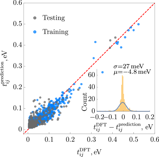
Figure 3: (Color online) Performance of the ensemble ANN model on the testing and training datasets for random split. The ensemble ANN shows $R^{2}=0.7$, RMSE = 28 meV and MAE = 18 meV on the testing dataset and $R^{2}=0.9$, RMSE = 19 meV and MAE = 11 meV on the training dataset. The inset figure shows the distribution of the ensemble ANN model error for the test dataset with $\mu$ and $\sigma$ are mean value and standard deviation of the errors. The solid line corresponds to the normal distribution with parameters $\mu$ and $\sigma$.

4 Transfer Integral Prediction

Our high-throughput DFT calculations yielded $N=1800$ local crystal environments $\{\vec{D}\}$ with corresponding transfer integrals $\{t_{ij}\}$. We build the ML model to predict the continuous-valued attribute $t_{ij}$ associated with the local crystal environment descriptor $\vec{D}$. To solve this regression problem, we tested the following models: (i) linear (LIR), (ii) random forest (RFR) Breiman_2001 regression models, and (iii) ANN. To achieve robust generalization and stability of the models, we employ the bagging (bootstrap aggregating) ensemble technique breiman1996bagging . The main idea behind bagging is to train multiple instances of the same model on different subsets of the training data and then combine their predictions to make the final estimation. For each model in the ensemble, a random sample is drawn with a replacement from the original training dataset. Thus, some data points may appear multiple times in the sample, while others may be left out. When making predictions, the individual predictions from each model are combined using a voting method (for classification tasks) or averaging (for regression tasks). In the work, we employ ensemble models with 100 estimators.

As a metric for the ensemble regression model performance with predictions $\tau$ we use: (i) the coefficient of determination

$$R^{2}=1-\dfrac{S_{\textsc{reg}}}{S_{\textsc{tot}}},$$ (7)

where $S_{\textsc{reg}}=\sum_{p=1}^{M}(t^{p}_{ij}-\tau^{p})^{2}$ is a sum of squared residuals of the regression model and $S_{\textsc{tot}}=\sum_{p=1}^{M}(t^{p}_{ij}-\overline{t_{ij}})^{2}$ is a total sum of squares with $\overline{t_{ij}}$ being the mean value of transfer integral in the test dataset with $M$ samples.

(ii) the root mean squared error (RMSE)

$$\text{RMSE}=\sqrt{\dfrac{1}{M}\sum_{p=1}^{M}(t^{p}_{ij}-\tau^{p})^{2}},$$ (8)

and (iii) mean absolute error

$$\text{MAE}=\dfrac{1}{M}\sum_{p=1}^{M}|t^{p}_{ij}-\tau^{p}|.$$ (9)

For RMSE, squared errors of the model are included in the average, making this measure more sensitive to outliers. As more variance in predictions, a larger RMSE. The MAE provides a mean of linear scores with all errors weighted equally.

Model	$\overline{R^{2}}$	$\overline{\text{RMSE}}$, meV	$\overline{\text{MAE}}$, meV
LIR	0.27 $\pm$ 0.18	44 $\pm$ 5	28 $\pm$ 1
RFR	0.59 $\pm$ 0.01	34 $\pm$ 3	21 $\pm$ 1
ANN	0.69 $\pm$ 0.05	29 $\pm$ 3	18 $\pm$ 1

Table 1: Results of shuffle-split CV of the selected ensemble models. The average value of $R^{2}$, RMSE, and MAE on six splits is given alongside the standard deviation.

Model	$\overline{R^{2}}$	$\overline{\text{RMSE}}$, meV	$\overline{\text{MAE}}$, meV
LIR	0.27 $\pm$ 0.20	43 $\pm$ 6	28 $\pm$ 1
RFR	0.57 $\pm$ 0.06	34 $\pm$ 5	21 $\pm$ 1
ANN	0.69 $\pm$ 0.10	28 $\pm$ 3	18 $\pm$ 1

Table 2: Results of $k$-fold CV of the selected ensemble models with six folds. The average value of $R^{2}$, RMSE, and MAE is given alongside the standard deviation.

For model selection, we employ two CV strategies: the shuffle-split and $k$-fold. In the shuffle-split, the dataset is randomly shuffled and then split into training and test subsets containing a specific percentage of the original data. The procedure is repeated the specified number of iterations. In each iteration the model is trained and evaluated accordingly. The shuffle-split procedure was implemented using the scikit-learn library scikit-learn with six splits, a test size of 20 %, and a training size of 80 % of the entire dataset. The results of the CV are presented in the Table 1. The model selection procedure shows that ensemble ANN has the best performance among the selected models. In particular, ensemble ANN has the lowest average errors, $\overline{\text{MAE}}$ = 18 meV and $\overline{\text{RMSE}}$ = 29 meV with the standard deviation of 1 and 3 meV respectively.

In the $k$-fold CV, the entire dataset is split into $k$ approximately equal parts (folds). Each ML model is trained on the $k-1$ folds and evaluated on one fold. The $k$-fold procedure was implemented using the scikit-learn library scikit-learn with $k=6$. The results of the $k$-fold CV are presented in Table 2. Similarly to the shuffle-split CV, $k$-fold CV shows that the ensemble ANN has the best scores with $\overline{\text{MAE}}$ = 18 meV and $\overline{\text{RMSE}}$ = 28 meV with the standard deviation of 1 and 3 meV respectively.

We also evaluated the ANN model on the random test-train split with 20 % of the data allocated for the test subset. The prediction of transfer integrals for the test set is shown in Fig. 3 as a scatter plot of the calculated values versus predicted ones.

5 Discussion

In this section, we will apply our ensemble ANN model to different classes of cuprates and discuss its predictive power. The first example are parent compounds of high-temperature superconductors (HTSC). The common structural feature of these antiferromagnets are cuprate planes formed by corner-sharing CuO₄ plaquettes. The Cu-O-Cu angle amounts to 180^∘, maximizing electron transfer between the nearest neighbors ($t_{1}$) and giving rise to a sizable antiferromagnetic exchange of about 1500 K coldea01 . In addition, the favorable mutual orientation of plaquettes boosts the coupling between second neighbors ($t_{2}$), as confirmed experimentally tanaka04 . Hence, the magnetic properties of undoped HTSC cuprates are described by the frustrated square-lattice model, with competing first- and second-neighbor antiferromagnetic exchanges. Interestingly, ramifications of this competition go far beyond the magnetism: the $t_{2}/t_{1}$ ratio shows correlations with the superconducting transition temperature Pavarini2001 . Thus, an accurate estimation of this ratio is crucial for understanding the physics of HTSC materials.

To test the accuracy of our ensemble ANN model, we consider the following parent HTSC compounds: La₂CuO₄, Bi₂Sr₂CuO₆, Tl₂Ba₂CuO₆, HgBa₂CuO₄, Tl₂Ba₂CaCu₂O₈, HgBa₂CaCu₂O₆, and HgBa₂Ca₂Cu₃O₈. It is important to note that only the former four structures were included in the training dataset. For all compounds, we recover the frustrated square lattice model with a dominant $t_{1}$ and a considerably smaller $t_{2}$. For ease of comparison with Ref. Pavarini2001 , we plot the resulting $t_{2}/t_{1}$ ratios as a function of the distance between Cu and the apical oxygen atom ($d_{\text{a}}$) in Fig. 4(a). In the same plot, we show the results of direct calculations of these transfer integrals by DFT calculations and Wannierization. A very good agreement is found for all seven cases.

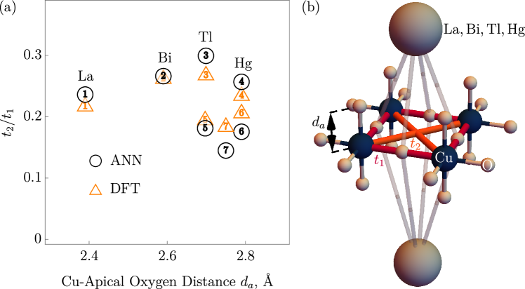
Figure 4: (Color online) (a) The $t_{2}/t_{1}$ ratio as a function of Cu - apical oxygen distance $d_{a}$ for HTSC cuprates. Black circles corresponds to the predictions of ensemble ANN model, and orange triangles – results of the DFT calculations. Numbers correspond to the following compounds: 1-Tl₂Ba₂Ca₂Cu₃O₁₀, 2-La₂CuO₄, 3-Bi₂Sr₂CuO₆, 4-Tl₂Ba₂CuO₆, 5-HgBa₂CuO₄, 6-Tl₂Ba₂CaCu₂O₈, 7-HgBa₂CaCu₂O₆, 8-HgBa₂Ca₂Cu₃O₈. (b) Schematics of the distinct structural element of the HTSC cuprate hosting leading $t_{1}$ and considerably smaller $t_{2}$ transfer integrals.

The closely related family of double-perovskite cuprates A₂CuTO₆ (A = Ba or Sr, T = Te or W) represents a more challenging test case. Here, the $t_{2}/t_{1}$ ratio crucially depends on the nature of the T atom: in the two Te-containing compounds, the leading coupling follows the shortest connections ($t_{1}$), while in the other two compounds the empty $5d$ shell of W boosts the diagonal coupling ($t_{2}$) katukuri20 . The sensitivity of our ANN model does not suffice to fully account for this trend: it yields a dominant $t_{2}$ for all four compounds. Despite this shortcoming, the model correctly reproduces the $t_{1}$-$t_{2}$ model, and the predicted $t_{2}/t_{1}$ ratio is lower for Te-containing (1.55 for Sr₂CuTeO₆ and 1.3 for Ba₂CuTeO₆) than for W-containing (1.6 for Sr₂CuTeO₆ and 1.95 for Ba₂CuWO₆) compounds.

Next, we turn to quasi-one-dimensional cuprates. The dominance of $t_{1}$ is correctly reproduced for the quasi-one-dimensional Sr₂CuO₃ rosner97 , another compound with corner-sharing connections between CuO₄ squares. Importantly, this structure features one shorter Cu-Cu connection, which is not accompanied by sizable electron transfer, and our model correctly captures this aspect: the respective predicted transfer integral is about 20 times smaller than the leading intra-chain term. For another quasi-one-dimensional compound, linarite PbCuSO₄(OH)₂ featuring edge-sharing chains, our model correctly recognizes the relevance of first- and second-neighbor transfer integrals along the chains, and correctly identifies the leading interchain coupling heinze22 . Importantly, in linarite like in many other edge-sharing cuprates, the nearest-neighbor exchange is ferromagnetic. Such exchanges have a more complex nature and can not be described within the effective one-orbital model, which is at the core of our approach. However, the presence of an edge-sharing connection essentially implies the relevance of the respective magnetic exchange, making a dedicated estimation of the electron transfer unnecessary.

As a less trivial case, we consider two isostructural natural minerals in which Cu²⁺ atoms form a kagome lattice: kapellasite $\alpha$-Cu₃Zn(OH)₆Cl₂ and haydeeite $\alpha$-Cu₃Mg(OH)₆Cl₂. The relevance of the cross-hexagon coupling $t_{d}$ and the corresponding magnetic exchange was suggested based on DFT results janson08 ; jeschke13 and confirmed experimentally fak12 ; boldrin15 . (As a side note, the $J_{d}$ exchange is the principal source of frustration in these systems, because the nearest-neighbor exchange $J_{1}$ is ferromagnetic.) Here, we consider crystal structures of kapellasite and haydeeite that were determined by neutron diffraction; these structures are not in the ICSD and hence were not used for training. The ANN model yields nearly identical results for both materials, suggesting the leading $t_{1}\simeq 78$ meV, plus sizable $t_{2}$ and $t_{d}$ of about 25 meV each. The $t_{1}$ and $t_{d}$ values are comparable with the first-principles calculations janson08 . Given that the latter used a different functional and a different structural input, the agreement is very good. Yet, the relevance of $t_{2}$ in the ensemble ANN model is a spurious result which is at odds with the DFT calculations and experiments.

In all previous examples except Sr₂CuO₃, the electronic structure featured several relevant transfer integrals. There are many cuprates whose magnetism is shaped by a single coupling dominating over other terms, but it is unclear which coupling is dominant. An instructive example is the spin-dimer compound Cu₂TeO₅, where magnetic dimers do not coincide with the structural ones das08 ; ushakov09 . For this material, our ANN model successfully reproduces the magnitude of the strongest coupling and its dominance over other terms. Another relevant example is the spin-chain compound CuSe₂O₅ janson2009 , where electron transfer is facilitated by the $[$Se₂O${}_{5}]^{2-}$ anionic group connecting two CuO₄ squares that are at an angle to each other. Also here the ANN model correctly identifies the leading transfer integral.

Naturally, the predictive power of the model is limited, and in some cases the desired accuracy is not reached. For instance, in Bi₂CuO₄ the leading coupling operates between the structural chains formed by stacks of CuO₄ squares, while the nearest-neighbor coupling within these stacks is three times weaker janson07 . Our ANN model correctly reproduces the leading coupling, yet predicts that the nearest-neighbor coupling has a similar strength. While the structure of ANN does not allow us to unequivocally determine the root cause of this discrepancy, we believe that it stems from the correlation between the magnitude of the transfer integral and the Cu..Cu separation. While on the average shorter distances indeed correspond to larger $\|t\|$, in some materials like Bi₂CuO₄ it is not the case.

There are several ways to improve the accuracy of the model. An apparent solution is to extend the dataset by including structures that are not represented in the ICSD. Also a revision of materials that were filtered out due to failed Wannierization can make the dataset bigger. However, such amendments will lead to incremental, moderate improvement of the predictive power. Based on our analysis, we conclude that main factor limiting the accuracy of the model are the crystalline environments descriptors. Making them more specific to chemical environments, e.g. by taking the connectivity of atoms within a chosen sphere into account or a more explicit consideration of charge densities, and keeping them as compact as possible may significantly improve the performance of the model.

To finalize the discussion, we emphasize that the main strength our model is its ability to identify magnetically relevant couplings. This is particularly useful for involved structures with a large number of short- and middle-range Cu..Cu separations, where the leading electron transfer paths can be highly nontrivial. The performance remains good across different classes of cuprates, which allows for efficient screening: evaluation of transfer integrals for a single material takes between dozens of seconds and a few minutes. Naturally, our model can not serve as a complete replacement to full-blown first-principle calculations, because error bars for the individual terms may be too high for certain quantitative analyses. However, the model’s predictive power is enough to perform qualitative assessment of interactions in spin models. Furthermore, the developed model holds substantial promise for enabling the inverse construction of hypothetical materials with prescribed magnetic topologies. For instance, one can create a Cu-O+X network and manipulate its structure to achieve a particular magnetic coupling arrangement, as indicated by the transfer integrals data generated by the model. Alternatively, one can begin with a known material and inquire about the alterations needed to activate or deactivate, as well as strengthen or weaken, specific magnetic connections. This then opens a plethora of questions on how these enhanced properties may be received in an actual chemical solid-state structure. Thereby this method may offer a novel avenue to engineer materials with distinct magnetic properties and unlock these applications, for instance in the fields of magnetic cooling or data storage.

6 Conclusions

We constructed an ensemble deep learning model that estimates the magnitude of transfer integrals in undoped cuprates. These terms underlie the leading mechanism of the magnetic exchange, and their knowledge is crucial for correctly determining the microscopic magnetic model. We employed a mapping onto a three-dimensional Zernike descriptor to describe crystalline environments that correspond to individual transfer integrals. The resulting ANN model trained on our high-throughput DFT calculations results can predict transfer integrals with reasonable error MAE = 18 meV. The model efficiently differentiates between weak and sizable transfer integrals, which is most important for estimating the relevant spin model. We discuss the limitations of this approach and outline ways of improving the numerical accuracy.

Acknowledgments We thank Markus Wallerberger, Roman Rezaev, and Dmitry Chernyavsky for fruitful discussions. This project was funded by the Leibniz Association through the Leibniz Competition. Authors acknowledge financial support from the DFG through the Collaborative Research Center SFB 1143 (Project-Id247310070). We thank Ulrike Nitzsche for the technical assistance.

Methods

DFT calculations For high-throughput DFT calculations, we used the crystal structures of cuprates downloaded from the ICSD bergerhoff.crystallographic.1987 employing the application programming interface (API). We performed nonmagnetic DFT calculations with the full potential local orbital code FPLO of version 18.00-52 koepernik.prb.1999 . Electron exchange-correlation interactions were described using the Perdew-Burke-Ernzerof (PBE) GGA functional perdew.prl.1996 . The electron density was converged to within 10^-6. The reciprocal space mesh was calculated for each structure, accounting for the size of the reciprocal cell suppl .

One shot calculation of Hellmann–Feynman forces was performed for each cuprate structure. We performed the relaxation of structures containing hydrogen by optimizing atomic coordinates of all H atoms with respect to the GGA total energy. All symmetries of the respective space group were kept during the optimization. The Wannier fit of the band structure was performed only for those structures where calculated forces are below 0.1 eV/Å suppl .

The Python library pymatgen Ong2013pymatgen has been used broadly in the high-throughput pipeline code to achieve complete automation.

Machine learning model In the work we consider regression problem $t_{ij}=f(\vec{D})$ which we handle with ML methods. For selection of the predictive model we consider shuffle-split and $k$-fold CV. The CV procedures were implemented with scikit-learn Python library scikit-learn . The best performance was shown by the ensemble ANN model. We implemented ANN using the Keras API chollet2015keras written in Python for learning platform Tensorflow tensorflow2015-whitepaper . The Supplementary Information 1 suppl provides the details on the architecture and training process of the ensemble ANN.

References

- \bibcommenthead
- (1) M. Tsubaki, T. Mizoguchi, Quantum Deep Field: Data-Driven Wave Function, Electron Density Generation, and Atomization Energy Prediction and Extrapolation with Machine Learning. Phys. Rev. Lett. 125, 206401 (2020).
- (2) S. L. Brunton, B. R. Noack, P. Koumoutsakos, Machine Learning for Fluid Mechanics. Annu. Rev. Fluid Mech. 52(1), 477–508 (2020).
- (3) J. Schmidt, M. R. G. Marques, S. Botti, M. A. L. Marques, Recent advances and applications of machine learning in solid-state materials science. npj Comput. Mater. 5(1), 83 (2019).
- (4) T. Xie, J. C. Grossman, Crystal Graph Convolutional Neural Networks for an Accurate and Interpretable Prediction of Material Properties. Phys. Rev. Lett. 120, 145301 (2018).
- (5) M. Rupp, A. Tkatchenko, K. R. Müller, O. A. von Lilienfeld, Fast and Accurate Modeling of Molecular Atomization Energies with Machine Learning. Phys. Rev. Lett. 108, 058301 (2012).
- (6) K. T. Schütt, H. Glawe, F. Brockherde, A. Sanna, K. R. Müller, E. K. U. Gross, How to represent crystal structures for machine learning: Towards fast prediction of electronic properties. Phys. Rev. B 89(20), 205118 (2014).
- (7) A. P. Bartók, R. Kondor, G. Csányi, On representing chemical environments. Phys. Rev. B 87(18), 184115 (2013).
- (8) A. Ziletti, D. Kumar, M. Scheffler, L. M. Ghiringhelli, Insightful classification of crystal structures using deep learning. Nat. Commun. 9(1), 2775 (2018).
- (9) V. Venkatraman, P. R. Chakravarthy, D. Kihara, Application of 3D Zernike descriptors to shape-based ligand similarity searching. J. Cheminformatics 1(1), 19 (2009).
- (10) M. Novotni, R. Klein, in Proceedings of the eighth ACM symposium on Solid modeling and applications - SM '03 (ACM Press, 2003).
- (11) M. Novotni, R. Klein, Shape retrieval using 3D Zernike descriptors. Comput. Aided Des. 36(11), 1047–1062 (2004).
- (12) L. Sael, B. Li, D. La, Y. Fang, K. Ramani, R. Rustamov, D. Kihara, Fast protein tertiary structure retrieval based on global surface shape similarity. Proteins: Structure, Function, and Bioinformatics 72(4), 1259–1273 (2008).
- (13) L. Mak, S. Grandison, R. J. Morris, An extension of spherical harmonics to region-based rotationally invariant descriptors for molecular shape description and comparison. J. Mol. Graph. Model. 26(7), 1035–1045 (2008).
- (14) L. Sael, D. La, B. Li, R. Rustamov, D. Kihara, Rapid comparison of properties on protein surface. Proteins: Struct. Funct. Genet. 73(1), 1–10 (2008).
- (15) N. Plakida, High-temperature cuprate superconductors, 2010th edn. Springer Series in Solid-State Sciences (Springer, Berlin, Germany, 2010).
- (16) T. Saha-Dasgupta, The Fascinating World of Low-Dimensional Quantum Spin Systems: Ab Initio Modeling. Molecules 26(6), 1522 (2021).
- (17) J. S. Helton, K. Matan, M. P. Shores, E. A. Nytko, B. M. Bartlett, Y. Yoshida, Y. Takano, A. Suslov, Y. Qiu, J. H. Chung, D. G. Nocera, Y. S. Lee, Spin Dynamics of the Spin-1/2 Kagome Lattice Antiferromagnet ZnCu3(OH)6Cl2. Phys. Rev. Lett. 98, 107204 (2007).
- (18) M. Jaime, V. F. Correa, N. Harrison, C. D. Batista, N. Kawashima, Y. Kazuma, G. A. Jorge, R. Stern, I. Heinmaa, S. A. Zvyagin, Y. Sasago, K. Uchinokura, Magnetic-Field-Induced Condensation of Triplons in Han Purple Pigment BaCuSi2O6. Phys. Rev. Lett. 93, 087203 (2004).
- (19) Y. Kohama, H. Ishikawa, A. Matsuo, K. Kindo, N. Shannon, Z. Hiroi, Possible observation of quantum spin-nematic phase in a frustrated magnet. Proc. Nat. Acad. Sci. 116, 10686–10690 (2019).
- (20) J. B. Goodenough, Magnetism And The Chemical Bond (John Wiley And Sons, 1963).
- (21) J. Hubbard, Electron correlations in narrow energy bands. Proc. R. Soc. Lond. A 276(1365), 238–257 (1963).
- (22) P. W. Anderson, New Approach to the Theory of Superexchange Interactions. Phys. Rev. 115, 2–13 (1959).
- (23) A. Auerbach, F. Berruto, L. Capriotti, Quantum Magnetism Approaches to Strongly Correlated Electrons (Springer Berlin Heidelberg, 2000), pp. 143–170.
- (24) A. Belik, M. Azuma, M. Takano, Characterization of quasi-one-dimensional S=1/2 Heisenberg antiferromagnets Sr2Cu(PO4)2 and Ba2Cu(PO4)2 with magnetic susceptibility, specific heat, and thermal analysis. J. Solid State Chem. 177(3), 883–888 (2004).
- (25) M. D. Johannes, J. Richter, S. L. Drechsler, H. Rosner, : A real material realization of the one-dimensional nearest neighbor Heisenberg chain. Phys. Rev. B 74, 174435 (2006).
- (26) O. Janson, W. Schnelle, M. Schmidt, Y. Prots, S. L. Drechsler, S. K. Filatov, H. Rosner, Electronic structure and magnetic properties of the spin-1/2 Heisenberg system CuSe2O5. New J. Phys. 11(11), 113034 (2009).
- (27) G. Bergerhoff, I. Brown, F. Allen, et al., Crystallographic databases. International Union of Crystallography, Chester 360, 77–95 (1987).
- (28) See Supplementary Information 1 for details of Wannierization, the reciprocal space mesh calculation, and the numerical implementation of functions and . See Supplementary Information 2 for the summary of Wannier fits.
- (29) S. P. Ong, W. D. Richards, A. Jain, G. Hautier, M. Kocher, S. Cholia, D. Gunter, V. L. Chevrier, K. A. Persson, G. Ceder, Python Materials Genomics (pymatgen): A robust, open-source python library for materials analysis. Comput. Mater. Sci. 68, 314–319 (2013).
- (30) J. P. Perdew, K. Burke, M. Ernzerhof, Generalized Gradient Approximation Made Simple. Phys. Rev. Lett. 77(18), 3865–3868 (1996).
- (31) K. Koepernik, H. Eschrig, Full-potential nonorthogonal local-orbital minimum-basis band-structure scheme. Phys. Rev. B 59(3), 1743–1757 (1999).
- (32) K. Koepernik, O. Janson, Y. Sun, J. van den Brink. Symmetry Conserving Maximally Projected Wannier Functions (2021). arXiv:2111.09652.
- (33) H. Eschrig, K. Koepernik, Tight-binding models for the iron-based superconductors. Phys. Rev. B 80, 104503 (2009).
- (34) N. Canterakis, Complete moment invariants and pose determination for orthogonal transformations of 3D objects. Internal Report 1/96, Technische Informatik I, Technische Universität Hamburg-Harburg (1996).
- (35) N. Canterakis, 3D Zernike moments and Zernike affine invariants for 3D image analysis and recognition. 11th Scandinavian Conference on Image Analysis (1999).
- (36) F. W. J. Olver, D. W. Lozier, R. F. Boisvert, C. W. Clark, NIST Handbook of Mathematical Functions (Cambridge University Press, 2010).
- (37) J. Morais, I. Cação, Quaternion Zernike spherical polynomials. Math. Comput. 84(293), 1317–1337 (2014).
- (38) L. Breiman, Random forests. Mach. Learn. 45(1), 5–32 (2001).
- (39) L. Breiman, Bagging predictors. Machine Learning 24(2), 123–140 (1996).
- (40) F. Pedregosa, G. Varoquaux, A. Gramfort, V. Michel, B. Thirion, O. Grisel, M. Blondel, P. Prettenhofer, R. Weiss, V. Dubourg, J. Vanderplas, A. Passos, D. Cournapeau, M. Brucher, M. Perrot, E. Duchesnay, Scikit-learn: Machine Learning in Python. J. Mach. Learn. Res. 12, 2825–2830 (2011).
- (41) R. Coldea, S. M. Hayden, G. Aeppli, T. G. Perring, C. D. Frost, T. E. Mason, S. W. Cheong, Z. Fisk, Spin waves and electronic interactions in . Phys. Rev. Lett. 86, 5377–5380 (2001).
- (42) K. Tanaka, T. Yoshida, A. Fujimori, D. H. Lu, Z. X. Shen, X. J. Zhou, H. Eisaki, Z. Hussain, S. Uchida, Y. Aiura, K. Ono, T. Sugaya, T. Mizuno, I. Terasaki, Effects of next-nearest-neighbor hopping on the electronic structure of cuprate superconductors. Phys. Rev. B 70, 092503 (2004).
- (43) E. Pavarini, I. Dasgupta, T. Saha-Dasgupta, O. Jepsen, O. K. Andersen, Band-structure trend in hole-doped cuprates and correlation with . Physical Review Letters 87(4) (2001).
- (44) V. M. Katukuri, P. Babkevich, O. Mustonen, H. C. Walker, B. Fåk, S. Vasala, M. Karppinen, H. M. Rønnow, O. V. Yazyev, Exchange interactions mediated by nonmagnetic cations in double perovskites. Phys. Rev. Lett. 124, 077202 (2020).
- (45) H. Rosner, H. Eschrig, R. Hayn, S. L. Drechsler, J. Málek, Electronic structure and magnetic properties of the linear chain cuprates and . Phys. Rev. B 56, 3402–3412 (1997).
- (46) L. Heinze, M. D. Le, O. Janson, S. Nishimoto, A. U. B. Wolter, S. Süllow, K. C. Rule, Low-energy spin excitations of the frustrated ferromagnetic chain material linarite PbCuSO4(OH)2 in applied magnetic fields parallel to the axis. Phys. Rev. B 106, 144409 (2022).
- (47) O. Janson, J. Richter, H. Rosner, Modified Kagome Physics in the Natural Spin-1/2 Kagome Lattice Systems: kapellasite Cu3Zn(OH)6Cl2 and Haydeeite Cu3Mg(OH)6Cl2. Phys. Rev. Lett. 101, 106403 (2008).
- (48) H. O. Jeschke, F. Salvat-Pujol, R. Valentí, First-principles determination of Heisenberg Hamiltonian parameters for the spin- kagome antiferromagnet ZnCu3(OH)6Cl2. Phys. Rev. B 88, 075106 (2013).
- (49) B. Fåk, E. Kermarrec, L. Messio, B. Bernu, C. Lhuillier, F. Bert, P. Mendels, B. Koteswararao, F. Bouquet, J. Ollivier, A. D. Hillier, A. Amato, R. H. Colman, A. S. Wills, Kapellasite: A Kagome Quantum Spin Liquid with Competing Interactions. Phys. Rev. Lett. 109, 037208 (2012).
- (50) D. Boldrin, B. Fåk, M. Enderle, S. Bieri, J. Ollivier, S. Rols, P. Manuel, A. S. Wills, Haydeeite: A spin- kagome ferromagnet. Phys. Rev. B 91, 220408 (2015).
- (51) H. Das, T. Saha-Dasgupta, C. Gros, R. Valentí, Proposed low-energy model Hamiltonian for the spin-gapped system . Phys. Rev. B 77, 224437 (2008).
- (52) A. V. Ushakov, S. V. Streltsov, Electronic and magnetic structure for the spin-gapped system CuTe2O5. J. Phys.: Condens. Matter 21, 305501 (2009).
- (53) O. Janson, R. O. Kuzian, S. L. Drechsler, H. Rosner, Electronic structure and magnetic properties of the spin-1/2 Heisenberg magnet Bi2CuO4. Phys. Rev. B 76, 115119 (2007).
- (54) F. Chollet, et al. Keras. https://keras.io (2015).
- (55) M. Abadi, A. Agarwal, P. Barham, E. Brevdo, Z. Chen, C. Citro, G. S. Corrado, A. Davis, J. Dean, M. Devin, S. Ghemawat, I. Goodfellow, A. Harp, G. Irving, M. Isard, Y. Jia, R. Jozefowicz, L. Kaiser, M. Kudlur, J. Levenberg, D. Mané, R. Monga, S. Moore, D. Murray, C. Olah, M. Schuster, J. Shlens, B. Steiner, I. Sutskever, K. Talwar, P. Tucker, V. Vanhoucke, V. Vasudevan, F. Viégas, O. Vinyals, P. Warden, M. Wattenberg, M. Wicke, Y. Yu, X. Zheng. TensorFlow: Large-scale machine learning on heterogeneous systems (2015). Software available from tensorflow.org.