Continuification control of large-scale multiagent systems under limited sensing and structural perturbations

Abstract

We investigate the stability and robustness properties of a continuification-based strategy for the control of large-scale multiagent systems. Within continuation-based strategy, one transforms the microscopic, agent-level description of the system dynamics into a macroscopic continuum-level, for which a control action can be synthesized to steer the macroscopic dynamics towards a desired distribution. Such an action is ultimately discretized to obtain a set of deployable control inputs for the agents to achieve the goal. The mathematical proof of convergence toward the desired distribution typically relies on the assumptions that no disturbance is present and that each agent possesses global knowledge of all the others’ positions. Here, we analytically and numerically address the possibility of relaxing these assumptions for the case of a one-dimensional system of agents moving in a ring. We offer compelling evidence in favor of the use of a continuification-based strategy when agents only possess a finite sensing capability and spatio-temporal perturbations affect the macroscopic dynamics of the ensemble. We also discuss some preliminary results about the role of an integral action in the macroscopic control solution.

I Introduction

Continuification (or continuation) control was first proposed in [1] as a viable approach to control the collective behavior of large-scale multiagent systems. The key idea of continuification consists of three fundamental steps: (i) finding a macroscopic description (typically a partial differential equation, PDE) for the collective dynamics of the multiagent system of interest; (ii) designing a macroscopic control action to attain the desired collective response; (iii) discretize the macroscopic control action to obtain feasible control inputs for the agents at the microscopic level.

This methodology tackles problems in which the control goal is formulated at the macroscopic collective dynamics level, but control actions are ultimately exerted only at the microscopic agent scale [2]. Applications of the approach are related, but not limited to, multi-robot systems [3, 4, 5, 6], cell populations [7, 8, 9], neuroscience [10, 11], and human networks [12, 13].

Such an approach was used in [14] to control the distribution of a multiagent system swarming in a ring, leading to an effective control scheme for the multiagent system to achieve a desired distribution. Crucially, to prove convergence of the macroscopic collective dynamics towards the desired distribution, two key assumptions were made. First, that agents possess unlimited sensing capabilities so as to know the positions of all other agents in the swarm. Second, that no disturbance or perturbation is affecting the agents dynamics.

The aim of this paper is to remove these unrealistic assumptions and study the performance, stability, and robustness of the continuification approach in the presence of limited sensing capabilities of the agents, spatio-temporal disturbances, or perturbations of their interaction kernel. In particular, we prove that local asymptotic or bounded convergence can still be achieved under these circumstances. As we undertake this task, we offer insight into the role of the control parameters on the size and shape of the region of asymptotic stability (or basin of attraction) of the desired distribution.

After providing some useful notation and mathematical preliminaries in Section II, we briefly recall the approach of [14] in Section III. Then, we assess the robustness properties of the continuification control approach in Sections IV and V. Finally, in Section VI, we show some preliminary results on the use of an additional integral action at the macroscopic level to improve the robustness of the microscopic dynamics, in the presence of perturbations or limited sensing. Theoretical results are complemented by numerical simulations.

II Mathematical preliminaries

Here, we offer some useful notation and mathematical concepts that will be used throughout the paper.

Definition 1 (Unit circle).

We define $\mathcal{S}:=[-\pi,\pi]$ as the unit circle.

Definition 2 ($L^{p}$-norm on $\mathcal{S}$ [15]).

Given a scalar function of $\mathcal{S}$ and time $h:\mathcal{S}\times\mathbb{R}_{\geq 0}\rightarrow\mathbb{R}$, we define its $L^{p}$-norm on $\mathcal{S}$ as

$$\|h(\cdot,t)\|_{p}:=\left(\int_{\mathcal{S}}|h(x,t)|^{p}\,\mathrm{d}x\right)^{1/p}.$$ (1)

For $p=\infty$,

$$\|h(\cdot,t)\|_{\infty}:=\mathrm{ess}\,\mathrm{sup}_{\mathcal{S}}|h(x,t)|.$$ (2)

For the sake of brevity, we denote these norms as $\|h\|_{p}$, without explicitly indicating their time dependencies.

Lemma 1 (Holder’s inequality [15]).

Given $n$ $L^{p}$ functions, $f_{i}\in L^{p}$, with $i=1,2,\dots n$,

$$\left\|\prod_{i=1}^{n}f_{i}\right\|_{1}\leq\prod_{i=1}^{n}\|f_{i}\|_{p_{i}},\;\;\mathrm{if}\;\;\sum_{i=1}^{n}\frac{1}{p_{i}}=1.$$ (3)

For instance, if $n=2$, we have $\|f_{1}f_{2}\|_{1}\leq\|f_{1}\|_{2}\|f_{2}\|_{2}$, as well as $\|f_{1}f_{2}\|_{1}\leq\|f_{1}\|_{1}\|f_{2}\|_{\infty}$.

We denote with “ $*$ ” the convolution operator. When referring to periodic domains and functions, the operator needs to be interpreted as a circular convolution [16].

Lemma 2 (Young’s convolution inequality [15]).

Given two functions, $f\in L^{p}$ and $g\in L^{q}$,

$$\|f*g\|_{r}\leq\|f\|_{p}\,\|g\|_{q},\;\;\mathrm{if}\;\;\frac{1}{p}+\frac{1}{q}=\frac{1}{r}+1,$$ (4)

where $1\leq p,q,r\leq\infty$. For instance, $\|f*g\|_{\infty}\leq\|f\|_{2}\|g\|_{2}$.

We denote with the subscripts $t$ and $x$ time and space partial differentiation, respectively. It can be shown [16] that the derivative of the convolution of two functions $(f*g)(x)$, can be computed as

$$(f*g)_{x}(x)=(f_{x}*g)(x)=(f*g_{x})(x).$$ (5)

Lemma 3 (Comparison lemma [17]).

Given a scalar ordinary differential equation (ODE) $v_{t}=f(t,v)$, with $v(t_{0})=v_{0}$, where $f$ is continuous in $t$ and locally Lipschitz in $v$, if a scalar function $u$ fulfills the differential inequality

$$u_{t}\leq f(t,u(t)),\;\;u(t_{0})\leq v_{0},$$ (6)

then

$$u(t)\leq v(t),\;\;\forall\,t\geq t_{0}.$$ (7)

III Continuification control

As in [14], we consider a group of $N$ identical mobile agents moving in $\mathcal{S}$. The dynamics of the $i$-th agent can be expressed as

$$\dot{x}_{i}=\sum_{j=1}^{N}f\left(\left\{x_{i},x_{j}\right\}_{\pi}\right)+u_{i},$$ (8)

where $x_{i}$ is the angular position of agent $i$ on $\mathcal{S}$, $\{x_{i},x_{j}\}_{\pi}$ is the angular distance between agents $i$ and $j$ wrapped on $\mathcal{S}$, $u_{i}$ is the velocity control input, and $f:\mathcal{S}\to\mathbb{R}$ is a periodic velocity interaction kernel modeling pairwise interactions between the agents [14].

Assuming the number of agents to be sufficiently large, the macroscopic collective dynamics can be adequately approximated through the mass balance equation [18]

$$\rho_{t}(x,t)+\left[\rho(x,t)V(x,t)\right]_{x}=q(x,t),$$ (9)

where $\rho:\mathcal{S}\times\mathbb{R}_{\geq 0}\to\mathbb{R}_{\geq 0}$ is the density profile of the agents on $\mathcal{S}$ at $t$ such that $\int_{\mathcal{S}}\rho(x,t)\,\mathrm{d}x=N$ for any $t$, and $V$ is the velocity field, which can be expressed as

$$V(x,t)=\int_{-\pi}^{\pi}f\left(\left\{x,y\right\}_{\pi}\right)\rho(y,t)\,\mathrm{d}y=(f*\rho)(x,t).$$ (10)

The function $q$ represents the macroscopic control input, which we first write as a mass source/sink to simplify derivations, but then recast as a controlled velocity field.

The boundary and initial conditions are given as follows:

$$\rho(-\pi,t)=\rho(\pi,t),\quad\forall t\geq 0,$$ (11)

$$\rho(x,0)=\rho^{0}(x),\quad\forall x\in\mathcal{S}.$$ (12)

We remark that $V$ is periodic by construction, as it comes from a circular convolution. This ensures that, in the open-loop scenario, when $q=0$, mass is conserved, that is $\mathrm{d}/\mathrm{d}t\int_{\mathcal{S}}\rho(x,t)\,\mathrm{d}x=0$ (integrating by parts).

Given some desired periodic smooth density profile, $\rho^{\text{d}}(x,t)$, associated with the target agents’ configuration, and such that $\|\rho^{\mathrm{d}}\|_{2}\leq M$ and $\|\rho^{\mathrm{d}}_{x}\|_{2}\leq L$ at any $t$, the continuification control problem is that of finding the control inputs $u_{i},\ i=1,2,\dots,N$ in (8) such that

$$\lim_{t\rightarrow\infty}\|{\rho^{\text{d}}(\cdot,t)}-\rho(\cdot,t)\|_{2}=0,$$ (13)

for agents starting from any initial configuration $x_{i}(0)=x_{i0},\ i=1,\ldots,N$.

To solve this problem, we first choose $q$ in (9) as

$$q(x,t)=K_{\mathrm{p}}e(x,t)-\left[e(x,t)V^{\mathrm{d}}(x,t)\right]_{x}\\ -\left[\rho(x,t)V^{\mathrm{e}}(x,t)\right]_{x},$$ (14)

where $K_{\mathrm{p}}$ is a positive control gain, $e=\rho^{\mathrm{d}}-\rho$, $V^{\text{d}}=(f*\rho^{\mathrm{d}})$, $V^{\text{e}}=(f*e)$, and we consider the reference dynamics

$$\rho^{\mathrm{d}}_{t}(x,t)+\left[\rho^{\mathrm{d}}(x,t)V^{\mathrm{d}}(x,t)\right]_{x}=0,$$ (15)

fulfilling initial and boundary conditions similar to (9). As shown in [14], such a choice ensures that the density $\rho$ globally asymptotically converges to $\rho^{\mathrm{d}}$.

Then, we recast the macroscopic controlled model (9) to include $q$ as a control action on the velocity field, that is,

$$\rho_{t}(x,t)+\left[\rho(x,t)(V(x,t)+U(x,t))\right]_{x}=0,$$ (16)

where $U$ is an auxiliary function computed from the linear PDE

$$\left[\rho(x,t)U(x,t)\right]_{x}=-q(x,t).$$ (17)

Integrating (17), we obtain (assuming $\rho\neq 0$)

$$U(x,t)=-\frac{1}{\rho(x,t)}\left[\int q(y,t)\,\mathrm{d}y+q(-\pi,t)\right].$$ (18)

Finally, we compute the velocity input acting on agent $i$ at the microscopic level by spatially sampling $U$ at $x_{i}$, that is,

$$u_{i}(t)=U(x_{i},t),\quad i=1,2,\ldots N.$$ (19)

The main limitation of this approach is the non-local nature of the control action. Since (14) is based on the convolution $V^{\mathrm{e}}$, agent $i$ must have global knowledge of $e$ to compute $u_{i}$. Moreover, as the choice of $q$ is based on some cancellations of the macroscopic dynamics of the system, the robustness to structural perturbations needs to be properly assessed. In this study, we address both of these issues.

IV Limited sensing capabilities

To relax the assumption of unlimited sensing, we assume agents can only sense an interval $[-\Delta,\Delta]$, with $\Delta>0$ centered at their position. The macroscopic control action in (14) becomes

$$\hat{q}(x,t)=K_{\mathrm{p}}e(x,t)-\left[e(x,t)V^{\mathrm{d}}(x,t)\right]_{x}\\ -\left[\rho(x,t)\hat{V}^{\mathrm{e}}(x,t)\right]_{x},$$ (20)

where $\hat{V}^{\mathrm{e}}=(\hat{f}*e)$, and $\hat{f}$ is a modified velocity interaction kernel defined as

$$\hat{f}(z)=f(z)\Pi(z,\Delta),$$ (21)

with $\Pi(z,\Delta)$ being a rectangular window of size $2\Delta$, centered at the origin.

Using $\hat{q}$ instead of $q$ as input to the macroscopic model (9) yields the following error dynamics:

$$e_{t}(x,t)=-K_{\mathrm{p}}e(x,t)+\left[\rho^{\mathrm{d}}(x,t)\tilde{V}(x,t)\right]_{x}\\ -\left[e(x,t)\tilde{V}(x,t)\right]_{x},$$ (22)

where $\tilde{V}=(g*e)$ and $g:=\hat{f}-f$.

Theorem 1 (LAS with limited sensing capabilities).

The error dynamics (22) locally asymptotically converges to 0.

Proof.

Choosing $\|e\|_{2}^{2}$ as a candidate Lyapunov function for (22), we get (omitting dependencies for simplicity)

$$(\|e\|_{2}^{2})_{t}=2\int_{\mathcal{S}}ee_{t}\,\mathrm{d}x=-2K_{\mathrm{p}}\|e\|_{2}^{2}-\int_{\mathcal{S}}e^{2}\tilde{V}_{x}\,\mathrm{d}x\\ +2\int_{\mathcal{S}}(e\rho^{\mathrm{d}}_{x}\tilde{V}+e\rho^{\mathrm{d}}\tilde{V}_{x})\,\mathrm{d}x,$$ (23)

where we computed product derivatives and used integration by parts taking into account the periodicity of the functions.

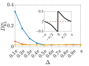
Figure 1: KL divergence at the end of a monomodal regulation trial, for different values of $\Delta$ and $K_{\mathrm{p}}$ ($K_{\mathrm{p}}=10$ in blue, $K_{\mathrm{p}}=100$ in orange and $K_{\mathrm{p}}=1000$ in yellow). In the inset, we show the repulsive interaction kernel.

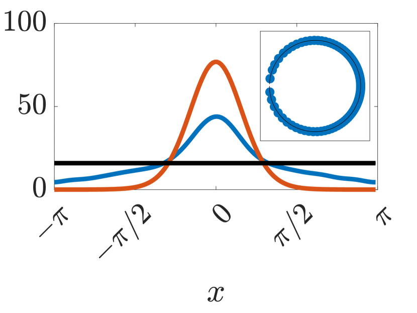
(a) $\Delta=0.1\pi$

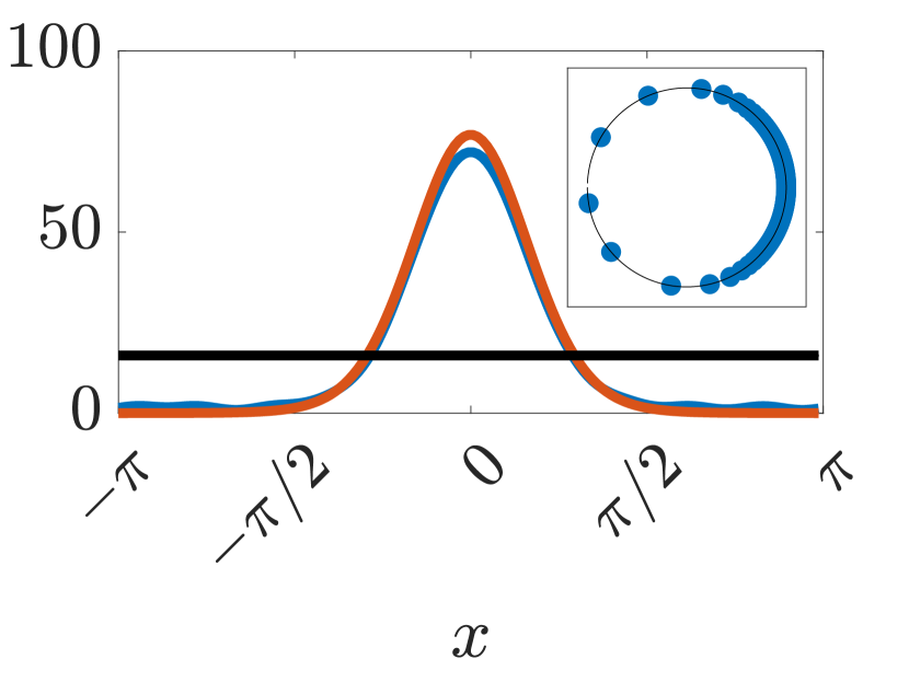
(b) $\Delta=0.4\pi$

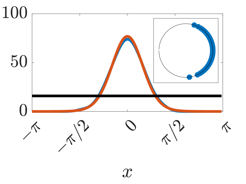
(c) $\Delta=0.7\pi$

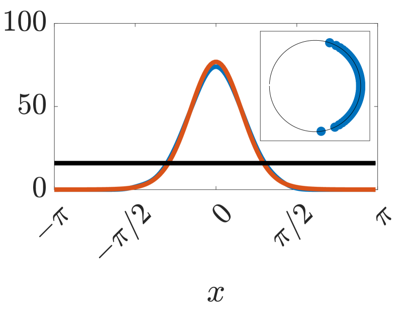
(d) $\Delta=\pi$

Figure 2: Steady-state ($t=t_{\mathrm{f}}$) comparison between the agents distribution (blue line) and the desired one (orange line) when the agents are started from the initial distribution (black line) for increasing sensing abilities of the agents when $K_{\mathrm{p}}=10$. Panel (d) shows the case when sensing is unlimited. In the inset of each panel, we display the discrete formation of the agents at the end of the trial.

Using the definition of $L^{1}$-norm (see Definition 2), applying Holder’s inequality with $n=3$, $p_{1}=p_{2}=2$, and $p_{3}=\infty$ (see Lemma 1), invoking Young’s convolution inequality with $r=\infty$ and $p=q=2$ (see Lemma 2), and recalling the assumption on the $L^{2}$ boundedness of $\rho^{\mathrm{d}}$ and $\rho^{\mathrm{d}}_{x}$ by constants $L$ and $M$, we find

$$\left|\int_{\mathcal{S}}e\rho^{\mathrm{d}}_{x}\tilde{V}\,\mathrm{d}x\right|\leq\int_{\mathcal{S}}|e\rho^{\mathrm{d}}_{x}\tilde{V}|\,\mathrm{d}x=\|e\rho^{\mathrm{d}}_{x}\tilde{V}\|_{1}\leq\\ \leq\|e\|_{2}\|\rho^{\mathrm{d}}_{x}\|_{2}\|\tilde{V}\|_{\infty}\leq L\|e\|_{2}^{2}\|g\|_{2},$$ (24)

$$\left|\int_{\mathcal{S}}e\rho^{\mathrm{d}}\tilde{V}_{x}\,\mathrm{d}x\right|\leq\int_{\mathcal{S}}|e\rho^{\mathrm{d}}\tilde{V}_{x}|\,\mathrm{d}x=\|e\rho^{\mathrm{d}}\tilde{V}_{x}\|_{1}\leq\\ \leq\|e\|_{2}\|\rho^{\mathrm{d}}\|_{2}\|\tilde{V}_{x}\|_{\infty}\leq M\|e\|_{2}^{2}\|g_{x}\|_{2},$$ (25)

$$\left|\int_{\mathcal{S}}e^{2}\tilde{V}_{x}\,\mathrm{d}x\right|\leq\int_{\mathcal{S}}|e^{2}\tilde{V}_{x}|\,\mathrm{d}x=\|ee\tilde{V}_{x}\|_{1}\leq\\ \leq\|e\|^{2}_{2}\|\tilde{V}_{x}\|_{\infty}\leq\|e\|^{3}_{2}\|g_{x}\|_{2}.$$ (26)

Using these bounds, from (23) we can write

$$(\|e\|_{2}^{2})_{t}\leq(-2K_{\mathrm{p}}+2M\|g_{x}\|_{2}+2L\|g\|_{2}+\|g_{x}\|_{2}\|e\|_{2})\|e\|_{2}^{2}.$$ (27)

Then, for any $\gamma>0$, if $\|e\|_{2}<\gamma$, the error asymptotically tends to the origin for $K_{\mathrm{p}}$ sufficiently large $\left[K_{\mathrm{p}}>(M+\gamma/2)\|g_{x}\|_{2}+L\|g\|_{2}\right]$, hence local asymptotic convergence is proved.

Numerical validation

We consider the same framework, control discretization and numerical set-up as in [14]. In particular, we refer to a mono-modal regulation scenario, where a repulsive swarm of $N=100$ agents, starting evenly displaced in $\mathcal{S}$, is required to achieve a desired density profile given by a von Mises function, with mean $\mu=0$ and concentration coefficient $k=4$. The pairwise interactions between agents is modelled via a repulsive Morse potential, depicted in the inset of Fig. 1, given by

$$f(x)=\mathrm{sign}(x)\left[-G\mathrm{e}^{-|x|/L}+\mathrm{e}^{-|x|}\right],$$ (28)

where the characteristic parameters, modulating the strength and characteristic distance of the attractive term, are $G=L=0.5$, making the repulsion term dominant.

We run several trials of duration $t_{\mathrm{f}}=6$. In each trial, we consider a different sensing radius $\Delta$, spanning from $0.1\pi$ to $\pi$. At the end of each trial, we record the steady-state Kullback-Leibler (KL) divergence between $\hat{\rho}$ and $\hat{\rho}^{\mathrm{d}}$ (equivalent to $\rho$ and $\rho^{\mathrm{d}}$, but normalized to sum to 1), $D_{\mathrm{KL}}^{\infty}$ [19]. The results of such a numerical investigation are reported in Fig. 1, for different values of $K_{\mathrm{p}}$. They show that: (i) for large values of $K_{\mathrm{p}}$, performance is independent from the specific sensing radius that is given to the agents, and (ii) for smaller values of $K_{\mathrm{p}}$, a limited knowledge of the domain can still guarantee a performance level that is comparable to the case of $\Delta=\pi$. For example, when considering $K_{\mathrm{p}}=10$, choosing $\Delta=0.4\pi$ makes $D_{\mathrm{KL}}^{\infty}$ comparable to the case of unlimited sensing capabilities. For the case $K_{\mathrm{p}}=10$, we also report in Fig. 2 the final configuration of the swarm (both in discrete and continuified terms) for different values of the sensing radius. We remark that the non-zero residual $D_{\mathrm{KL}}$ is due to the discretization process.

V Structural perturbations

Next, we assess the robustness of the approach to two classes of perturbations, the first acting additively on the macroscopic velocity field and the second on the interaction kernel.

V-A Spatio-temporal perturbations of the velocity field

We assume that perturbations of the microscopic dynamics can be captured at the macroscopic level by means of some spatio-temporal velocity field $d(x,t)$ affecting (9). The macroscopic controlled model becomes

$$\rho_{t}(x,t)+\left[\rho(x,t)(V(x,t)+d(x,t))\right]_{x}=q(x,t),$$ (29)

where we assume $d(-\pi,t)=d(\pi,t)$ for any $t$ and $d,d_{x}\in L^{\infty}$ at any $t$ so that that there exist two positive constants $D_{1}$ and $D_{2}$ bounding the $L^{\infty}$-norm of $d$ and $d_{x}$, respectively.

Substituting (14) into (29) and taking into account the reference dynamics (15) yields

$$e_{t}(x,t)=-K_{\mathrm{p}}e(x,t)+\left[(\rho^{\mathrm{d}}(x,t)-e(x,t))d(x,t)\right]_{x}.$$ (30)

Theorem 2 (Bounded convergence in the presence of velocity perturbations).

  There exists a threshold value $D_{2}<\kappa<+\infty$ such that, if $2K_{\mathrm{p}}>\kappa$, the dynamics of the squared error norm is bounded and

$$\lim_{t\rightarrow\infty}{\|e(\cdot,t)\|_{2}}\leq\frac{2LD_{1}+2MD_{2}}{\kappa-D_{2}}$$

Hence, the upper bound on the steady-state error can be made arbitrarily small by choosing $\kappa$ sufficiently large.

Proof.

Taking into account (30), we write the dynamics of $\|e\|_{2}^{2}$ (omitting dependencies for simplicity) as

$$(\|e\|_{2}^{2})_{t}=2\int_{\mathcal{S}}ee_{t}\,\mathrm{d}x=-2K_{\mathrm{p}}\|e\|_{2}^{2}-\int_{\mathcal{S}}e^{2}d_{x}\,\mathrm{d}x\\ +2\int_{\mathcal{S}}(e\rho_{x}^{\mathrm{d}}d+e\rho^{\mathrm{d}}d_{x})\,\mathrm{d}x,$$ (31)

where we computed product derivatives and applied integration by parts exploiting the periodicity of the functions. Similar to the proof of Theorem 1, we apply Definition 2, Holder’s inequality with $n=3$, $p_{1}=p_{2}=2$ and $p_{3}=\infty$ (see Lemma 1), and exploit the bounds on $\rho^{\mathrm{d}}$, $\rho^{\mathrm{d}}_{x}$, $d$ and $d_{x}$, to derive the following inequalities for the terms in (31):

$$\left|\int_{\mathcal{S}}e\rho^{\mathrm{d}}_{x}d\,\mathrm{d}x\right|\leq\int_{\mathcal{S}}|e\rho^{\mathrm{d}}_{x}d|\,\mathrm{d}x=\|e\rho^{\mathrm{d}}_{x}d\|_{1}\leq\\ \leq\|e\|_{2}\|\rho^{\mathrm{d}}_{x}\|_{2}\|d\|_{\infty}\leq LD_{1}\|e\|_{2},$$ (32)

$$\left|\int_{\mathcal{S}}e\rho^{\mathrm{d}}d_{x}\,\mathrm{d}x\right|\leq\int_{\mathcal{S}}|e\rho^{\mathrm{d}}d_{x}|\,\mathrm{d}x=\|e\rho^{\mathrm{d}}d_{x}\|_{1}\leq\\ \leq\|e\|_{2}\|\rho^{\mathrm{d}}\|_{2}\|d_{x}\|_{\infty}\leq MD_{2}\|e\|_{2},$$ (33)

$$\left|\int_{\mathcal{S}}e^{2}d_{x}\,\mathrm{d}x\right|\leq\int_{\mathcal{S}}|e^{2}d_{x}|\,\mathrm{d}x=\|eed_{x}\|_{1}\leq\\ \leq\|e\|_{2}^{2}\|d_{x}\|_{\infty}\leq D_{2}\|e\|_{2}^{2}.$$ (34)

Hence, we obtain

$$(\|e\|_{2}^{2})_{t}\leq\left(-2K_{\mathrm{p}}+D_{2}\right)\|e\|_{2}^{2}+\left(2LD_{1}+2MD_{2}\right)\|e\|_{2}.$$ (35)

Figure 3: Phase portrait of the system bounding $\|e\|_{2}^{2}$ in the presence of spatio-temporal disturbances.

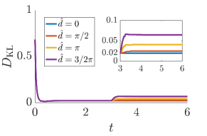
Figure 4: Time evolution of the KL divergence when a constant disturbance of amplitude $\hat{d}$ switches on at $t=3$. In the inset, a zoom of the second half of the trial.

For convenience, we rewrite (35) as

$$\eta_{t}\leq-a\eta+c\sqrt{\eta}:=h(\eta),$$ (36)

where $\eta=\|e\|_{2}^{2}$, $a=2K_{\mathrm{p}}-D_{2}$, and $c=2LD_{1}+2MD_{2}$. Under the assumption that $2K_{\mathrm{p}}>D_{2}$ ($a>0$), the phase portrait of the bounding field $h$ yield an asymptotically stable equilibrium at (see Fig. 3)

$$\frac{c^{2}}{a^{2}}=\frac{(2LD_{1}+2MD_{2})^{2}}{(2K_{\mathrm{p}}-D_{2})^{2}}$$

(with basin of attraction $\mathbb{R}_{>0}$). Thus, using Lemma 3, $\eta$ is bounded by $c^{2}/a^{2}$. Moreover, choosing $2K_{\mathrm{p}}>\kappa>D_{2}$, the stable equilibrium of the bounding field $h$ can be moved arbitrarily closer to the origin, thereby proving our claim.

Numerical validation

We consider the same scenario presented in the previous section but assuming that a disturbance $d(x,t)=\hat{d}w(t)$, where $\hat{d}$ is a constant and $w(t)=\mathrm{step}(t-t_{\mathrm{f}}/2)$, is acting on the macroscopic dynamics. Setting $K_{\mathrm{p}}=10$ and considering different values of $\hat{d}$, we obtain the results reported in Fig. 4. As expected, in the presence of the disturbances, the KL divergence remains bounded and decreases as the control gain $K_{\mathrm{p}}$ increases. For example, the steady-state value of the KL divergence decreases from 0.06 when $K_{\mathrm{p}}=10$ to less than 0.02 when $K_{\mathrm{p}}\geq 100$.

V-B Interaction kernel perturbation

Next, we consider the case where structural perturbations affect the interaction kernel. We assume that the interaction kernel, $\tilde{f}$, used to compute the macroscopic control action is different from the actual interaction kernel, $f$, influencing the agents’ motion. We compute the control input as

$$\tilde{q}(x,t)=K_{\mathrm{p}}e(x,t)-\left[e(x,t)\tilde{V}^{\mathrm{d}}(x,t)\right]_{x}\\ -\left[\rho(x,t)\tilde{V}^{\mathrm{e}}(x,t)\right]_{x},$$ (37)

where $\tilde{V}^{\mathrm{d}}=(\tilde{f}*\rho^{\mathrm{d}})$ and $\tilde{V}^{\mathrm{e}}=(\tilde{f}*e)$.

Substituting (37) into (9) and considering the reference dynamics (15), the error dynamics becomes

$$e_{t}(x,t)=-K_{\mathrm{p}}e(x,t)+\left[e(x,t)\tilde{U}^{\mathrm{d}}(x,t)\right]_{x}\\ +\left[\rho^{\mathrm{d}}(x,t)\tilde{U}^{\mathrm{e}}(x,t)\right]_{x}-\left[e(x,t)\tilde{U}^{\mathrm{e}}(x,t)\right]_{x},$$ (38)

where, letting $\tilde{g}=\tilde{f}-f$ be the mismatch between the interaction kernels, we have

$$\tilde{U}^{\mathrm{d}}(x,t)=\tilde{V}^{\mathrm{d}}(x,t)-V^{\mathrm{d}}(x,t)=(\tilde{g}*e)(x,t),$$ (39)

$$\tilde{U}^{\mathrm{e}}(x,t)=\tilde{V}^{\mathrm{e}}(x,t)+V^{\mathrm{e}}(x,t)=(\tilde{g}*e)(x,t).$$ (40)

Theorem 3 (LAS with kernel perturbation).

 The error dynamics (38) locally asymptotically converges to 0, if $\tilde{g},\tilde{g}_{x}\in L^{2}$.

Proof.

Assuming $\|e\|_{2}^{2}$ to be a candidate Lyapunov function for (38), we get

$$(\|e\|_{2}^{2})_{t}=\int_{\mathcal{S}}ee_{t}\,\mathrm{d}x=-2K_{\mathrm{p}}\|e\|_{2}^{2}-\int_{\mathcal{S}}e^{2}\tilde{U}^{\mathrm{e}}_{x}\,\mathrm{d}x\\ +\int_{\mathcal{S}}e^{2}\tilde{U}^{\mathrm{d}}_{x}\,\mathrm{d}x-2\int_{\mathcal{S}}(e\rho^{\mathrm{d}}_{x}\tilde{U}^{\mathrm{e}}+e\rho^{\mathrm{d}}\tilde{U}^{\mathrm{e}}_{x})\,\mathrm{d}x.$$ (41)

where we computed the product derivatives and used integration by parts by exploiting the fact that $\tilde{U}^{\mathrm{d}}$ and $\tilde{U}^{\mathrm{e}}$ are periodic by construction (they come from a circular convolution). Using similar arguments to those above, we can establish upper bounds for the terms in (41) as follows:

$$\left|\int_{\mathcal{S}}e\rho^{\mathrm{d}}_{x}\tilde{U}^{\mathrm{e}}\,\mathrm{d}x\right|\leq\int_{\mathcal{S}}|e\rho^{\mathrm{d}}_{x}\tilde{U}^{\mathrm{e}}|\,\mathrm{d}x=\|e\rho^{\mathrm{d}}_{x}\tilde{U}^{\mathrm{e}}\|_{1}\leq\\ \leq\|e\|_{2}\|\rho^{\mathrm{d}}_{x}\|_{2}\|\tilde{U}^{\mathrm{e}}\|_{\infty}\leq L\|\tilde{g}\|_{2}\|e\|_{2}^{2},$$ (42)

$$\left|\int_{\mathcal{S}}e\rho^{\mathrm{d}}\tilde{U}^{\mathrm{e}}_{x}\,\mathrm{d}x\right|\leq\int_{\mathcal{S}}|e\rho^{\mathrm{d}}\tilde{U}^{\mathrm{e}}_{x}|\,\mathrm{d}x=\|e\rho^{\mathrm{d}}\tilde{U}^{\mathrm{e}}_{x}\|_{1}\leq\\ \leq\|e\|_{2}\|\rho^{\mathrm{d}}\|_{2}\|\tilde{U}^{\mathrm{e}}_{x}\|_{\infty}\leq M\|\tilde{g}_{x}\|_{2}\|e\|_{2}^{2},$$ (43)

$$\left|\int_{\mathcal{S}}e^{2}\tilde{U}^{\mathrm{e}}_{x}\,\mathrm{d}x\right|\leq\int_{\mathcal{S}}|e^{2}\tilde{U}^{\mathrm{e}}_{x}|\,\mathrm{d}x=\|ee\tilde{U}^{\mathrm{e}}_{x}\|_{1}\leq\\ \leq\|e\|^{2}_{2}\|\tilde{U}^{\mathrm{e}}_{x}\|_{\infty}\leq\|\tilde{g}_{x}\|_{2}\|e\|^{3}_{2},$$ (44)

$$\left|\int_{\mathcal{S}}e^{2}\tilde{U}^{\mathrm{d}}_{x}\,\mathrm{d}x\right|\leq\int_{\mathcal{S}}|e^{2}\tilde{U}^{\mathrm{d}}_{x}|\,\mathrm{d}x=\|ee\tilde{U}^{\mathrm{d}}_{x}\|_{1}\leq\\ \leq\|e\|^{2}_{2}\|\tilde{U}^{\mathrm{d}}_{x}\|_{\infty}\leq\|e\|^{2}_{2}\|\|\rho^{\mathrm{d}}\|_{2}\|\tilde{g}_{x}\|_{2}\leq M\|\tilde{g}_{x}\|_{2}\|e\|^{2}_{2}.$$ (45)

Using these bounds in (41) we obtain

$$(\|e\|_{2}^{2})_{t}\leq(-2K_{\mathrm{p}}+3M\|\tilde{g}_{x}\|_{2}+2L\|\tilde{g}\|_{2}+\|\tilde{g}_{x}\|_{2}\|e\|_{2})\|e\|_{2}^{2}.$$ (46)

Then, for any $\gamma>0$, if $\|e\|_{2}<\gamma$, the error converges to 0, for $K_{\mathrm{p}}$ sufficiently large, namely, $K_{\mathrm{p}}>\|\tilde{g}_{x}\|_{2}\gamma/2+3M\|\tilde{g}_{x}\|_{2}/2+L\|\tilde{g}\|_{2}$.

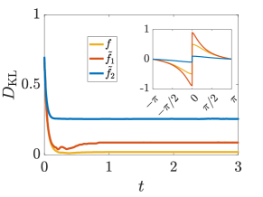
Figure 5: Time evolution of the KL divergence when the perturbed kernels $\tilde{f}_{1}$ and $\tilde{f}_{2}$ shown in the inset are used to compute the control action, instead of the nominal kernel $f$.

Numerical validation

We consider again the scenario used in Section IV but we assume that a perturbed kernel is used to compute the macroscopic control action $q$. Specifically, we test robustness against the two perturbed kernels $\tilde{f}_{1}$ and $\tilde{f}_{2}$, obtained by setting the characteristic parameters in (28) to $G=L=0.1$ and $G=L=0.9$, respectively.

Setting $K_{\mathrm{p}}=10$, we obtain results shown in Fig. 5 where we observe an increase in the steady-state mismatch between the distribution of the agents and the desired density as the kernel becomes more different than the nominal one ($\tilde{f}_{2}$ being the worst case). As expected from the analysis, our numerical results (omitted here of brevity) confirm that the steady-state mismatch decreases as $K_{\mathrm{p}}$ increases approaching the nominal case in [14].

VI Adding a macroscopic Integral action

In all the cases examined earlier, some bounded mismatch between the desired and steady-state distribution of the agents remains in the presence of perturbations. To resolve this issue, we explored the inclusion of an integral action in the form $K_{\mathrm{i}}\int_{0}^{\tau}e(x,\tau)\,\mathrm{d}\tau,$ with $K_{\mathrm{i}}$ being a positive control gain, to the macroscopic control law in (14).

Preliminary results in Fig. 6 indicate a substantial improvement of the steady-state error in all the considered scenarios (for brevity only two cases are shown). These findings point at the possibility to compensate for disturbances and perturbations within a continuification-based control strategy via an additional integral action. The analytical characterization of the effects of the macroscopic integral action is the subject of ongoing work and will be presented elsewhere.

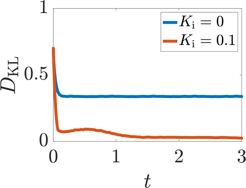
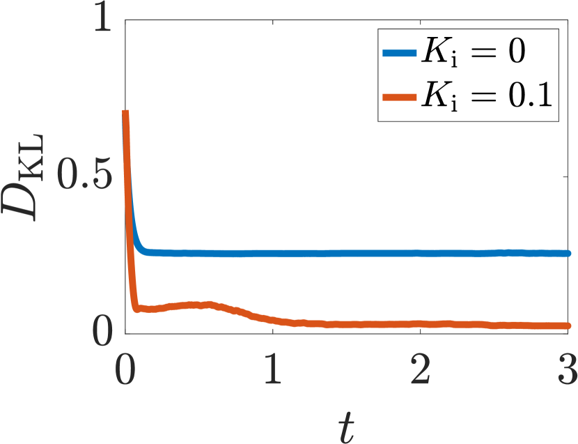
Figure 6: Effects of a macroscopic integral action when (a) agents possess limited sensing with $\Delta=0.1\pi$ and (b) when their interaction kernel is perturbed and set equal to $\tilde{f}_{2}$. We compare the cases of $K_{\mathrm{i}}=0$ and $K_{\mathrm{i}}=0.1$, for $K_{\mathrm{p}}=10$.

VII Conclusions

We investigated the stability and robustness properties of a continuification control strategy for a set of agents in a ring. We quantified the extent to which the approach presented in [14] is affected by key realistic effects, including (i) limited sensing capabilities of the agents; (ii) presence of spatio-temporal disturbances; and (iii) structural perturbations of their interaction kernel. In all cases, we establish the mathematical proofs of local asymptotic or bounded convergence – the latter in the form of a residual steady-state mismatch that can be made arbitrarily small by increasing the control gain. We also reported preliminary results about the addition of a spatio-temporal integral action at the macroscopic level that can considerably reduce the steady-state error, even after the action is discretized and deployed at the microscopic agents’ level. Ongoing work is aimed at analytically characterizing the effects of such an action and generalizing the approach to higher dimensions.

References

- [1] D. Nikitin, C. Canudas-de Wit, and P. Frasca, “A continuation method for large-scale modeling and control: From odes to pde, a round trip,” IEEE Transactions on Automatic Control, vol. 67, no. 10, pp. 5118–5133, 2022.
- [2] M. di Bernardo, “Controlling collective behavior in complex systems,” in Encyclopedia of Systems and Control, J. Baillieul and T. Samad, Eds. Springer London, 2020.
- [3] G. Freudenthaler and T. Meurer, “Pde-based multi-agent formation control using flatness and backstepping: Analysis, design and robot experiments,” Automatica, vol. 115, p. 108897, 2020.
- [4] S. Biswal, K. Elamvazhuthi, and S. Berman, “Decentralized control of multiagent systems using local density feedback,” IEEE Transactions on Automatic Control, vol. 67, no. 8, pp. 3920–3932, 2021.
- [5] J. Qi, R. Vazquez, and M. Krstic, “Multi-agent deployment in 3-d via pde control,” IEEE Transactions on Automatic Control, vol. 60, no. 4, pp. 891–906, 2014.
- [6] C. Sinigaglia, A. Manzoni, and F. Braghin, “Density control of large-scale particles swarm through pde-constrained optimization,” IEEE Transactions on Robotics, vol. 38, no. 6, pp. 3530–3549, 2022.
- [7] A. Guarino, D. Fiore, D. Salzano, and M. di Bernardo, “Balancing cell populations endowed with a synthetic toggle switch via adaptive pulsatile feedback control,” ACS Synthetic Biology, vol. 9, no. 4, pp. 793–803, 2020.
- [8] D. K. Agrawal, R. Marshall, V. Noireaux, and E. D. Sontag, “In vitro implementation of robust gene regulation in a synthetic biomolecular integral controller,” Nature Communications, vol. 10, no. 1, pp. 1–12, 2019.
- [9] A. Rubio Denniss, T. E. Gorochowski, and S. Hauert, “An open platform for high-resolution light-based control of microscopic collectives,” Advanced Intelligent Systems, p. 2200009, 2022.
- [10] T. Menara, G. Baggio, D. Bassett, and F. Pasqualetti, “Functional control of oscillator networks,” Nature Communications, vol. 13, no. 1, p. 4721, 2022.
- [11] R. Noori, D. Park, J. D. Griffiths, S. Bells, P. W. Frankland, D. Mabbott, and J. Lefebvre, “Activity-dependent myelination: A glial mechanism of oscillatory self-organization in large-scale brain networks,” Proceedings of the National Academy of Sciences, vol. 117, no. 24, pp. 13 227–13 237, 2020.
- [12] S. Shahal, A. Wurzberg, I. Sibony, H. Duadi, E. Shniderman, D. Weymouth, N. Davidson, and M. Fridman, “Synchronization of complex human networks,” Nature communications, vol. 11, no. 1, pp. 1–10, 2020.
- [13] C. Calabrese, M. Lombardi, E. Bollt, P. De Lellis, B. G. Bardy, and M. Di Bernardo, “Spontaneous emergence of leadership patterns drives synchronization in complex human networks,” Scientific Reports, vol. 11, no. 1, pp. 1–12, 2021.
- [14] G. C. Maffettone, A. Boldini, M. Di Bernardo, and M. Porfiri, “Continuification control of large-scale multiagent systems in a ring,” IEEE Control Systems Letters, vol. 7, pp. 841–846, 2023.
- [15] S. Axler, Measure, integration & real analysis. Springer Nature, 2020.
- [16] M. C. Jeruchim, P. Balaban, and K. S. Shanmugan, Simulation of communication systems: modeling, methodology and techniques. Springer Science & Business Media, 2006.
- [17] H. K. Khalil, Nonlinear systems. Patience Hall, 2002.
- [18] A. J. Bernoff and C. M. Topaz, “A primer of swarm equilibria,” SIAM Journal on Applied Dynamical Systems, vol. 10, no. 1, pp. 212–250, 2011.
- [19] S. Kullback and R. A. Leibler, “On information and sufficiency,” The Annals of Mathematical Statistics, vol. 22, no. 1, pp. 79–86, 1951.