CrOC : Cross-View Online Clustering for Dense Visual Representation Learning

Abstract

Learning dense visual representations without labels is an arduous task and more so from scene-centric data. We propose to tackle this challenging problem by proposing a Cross-view consistency objective with an Online Clustering mechanism (CrOC) to discover and segment the semantics of the views. In the absence of hand-crafted priors, the resulting method is more generalizable and does not require a cumbersome pre-processing step. More importantly, the clustering algorithm conjointly operates on the features of both views, thereby elegantly bypassing the issue of content not represented in both views and the ambiguous matching of objects from one crop to the other. We demonstrate excellent performance on linear and unsupervised segmentation transfer tasks on various datasets and similarly for video object segmentation. Our code and pre-trained models are publicly available at https://github.com/stegmuel/CrOC.

1 Introduction

Self-supervised learning (SSL) has gone a long and successful way since its beginning using carefully hand-crafted proxy tasks such as colorization [26], jigsaw puzzle solving [32], or image rotations prediction [14]. In recent years, a consensus seems to have been reached, and cross-view consistency is used in almost all state-of-the-art (SOTA) visual SSL methods [7, 19, 15, 5, 6]. In that context, the whole training objective revolves around the consistency of representation in the presence of information-preserving transformations [7], e.g., blurring, cropping, solarization, etc. Although this approach is well grounded in learning image-level representations in the unrealistic scenario of object-centric datasets, e.g., ImageNet [11], it cannot be trivially extended to accommodate scene-centric datasets and even less to learn dense representations. Indeed, in the presence of complex scene images, the random cropping operation used as image transformation loses its semantic-preserving property, as a single image can yield two crops bearing antipodean semantic content [31, 37, 35, 36]. Along the same line, it’s not clear how to relate sub-regions of the image from one crop to the other, which is necessary to derive a localized supervisory signal.

To address the above issue, some methods [31, 36] constrain the location of the crops based on some heuristics and using a pre-processing step. This step is either not learnable or requires the use of a pre-trained model.

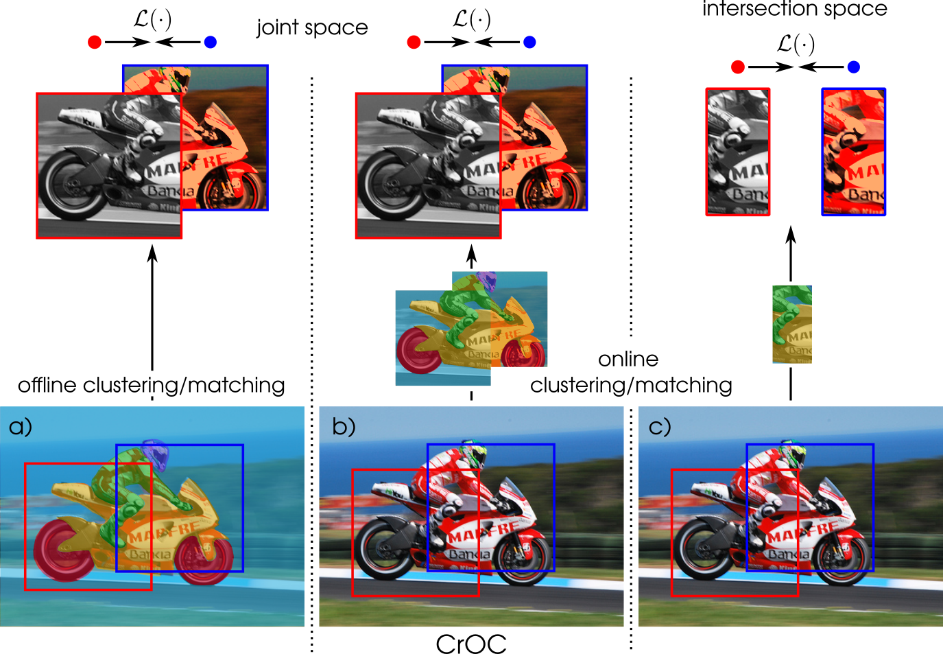
Figure 1: Schematic for different categories of self-supervised learning methods for dense downstream tasks. a) Prior to the training, a pre-trained model or color-based heuristic is used to produce the clustering/matching of the whole dataset. c) The matching/clustering is identified online but restrains the domain of application of the loss to the intersection of the two views. b) Our method takes the best of both worlds, leverages online clustering, and enforces constraints on the whole spatiality of the views.

Alternatively, the location of the crops (geometric pooling [51, 45]) and/or an attention mechanism (attentive pooling [51, 48, 33, 44, 42]) can be used to infer the region of overlap in each view and only apply the consistency objective to that region (Fig. 1.c). A consequence of these pooling mechanisms is that only a sub-region of each view is exploited, which mislays a significant amount of the image and further questions the usage of cropping. There are two strategies to tackle the issue of locating and linking the objects from the two views: the first is a feature-level approach that extends the global consistency criterion to the spatial features after inferring pairs of positives through similarity bootstrapping or positional cues [30, 48, 2, 41, 28, 51]. It is unclear how much semantics a single spatial feature embeds, and this strategy can become computationally intensive. These issues motivate the emergence of the second line of work which operates at the object-level [44, 20, 21, 47, 38, 40, 43]. In that second scenario, the main difficulty lies in generating the object segmentation masks and matching objects from one view to the other. The straightforward approach is to leverage unsupervised heuristics [20] or pre-trained models [47] to generate pseudo labels prior to the training phase (Fig. 1.a), which is not an entirely data-driven approach and cannot be trivially extended to any modalities. Alternatively, [21] proposed to use K-Means and an additional global image (encompassing the two main views) to generate online pseudo labels, but this approach is computationally intensive.

To address these limitations, we propose CrOC, whose underpinning mechanism is an efficient Cross-view Online Clustering that conjointly generates segmentation masks for the union of both views (Fig. 1.b).

Our main contributions are: 1) we propose a novel object-level self-supervised learning framework that leverages an online clustering algorithm yielding segmentation masks for the union of two image views. 2) The introduced method is inherently compatible with scene-centric datasets and does not require a pre-trained model. 3) We empirically and thoroughly demonstrate that our approach rivals or out-competes existing SOTA self-supervised methods even when pre-trained in an unfavorable setting (smaller and more complex dataset).

2 Related work

Global features. The collateral effect of [7], is that it effectively uniformized the choice of the proxy task for SSL to the extent that cross-view consistency is almost exclusively used. The remaining degree of freedom lies in the technique used to avoid the collapse to trivial solutions. The use of negative samples [7, 22] effectively and intuitively treats this degeneracy at the cost of using large batches, which can be mitigated by a momentum encoder [19]. At the other end of the spectrum, clustering-based approaches [1, 4, 5, 6] have shown that enforcing equipartition of the samples over a set of clusters was sufficient to palliate the collapsing issue.

Local features. Local methods aim at completing the image-level objective by encouraging cross-view consistency at a localized level such that the resulting features are well aligned with dense downstream tasks. Broadly speaking, these methods can be categorized by the granularity at which the similarity is enforced. The first category encompasses approaches [41, 30, 33, 27], where similarity is encouraged directly at the feature level, i.e., from one feature to the other. The difficulty lies in obtaining valid pairs or groups of features. To that end, various methods [41, 30] rely solely on the similarity of the features, whereas the matching criterion of [48, 33] is driven by their distances/positions. [27] studies both approaches and [2] incorporates both in a single objective.

The second category of methods [8, 44, 20, 21, 47] enforce consistency at a higher level, which first requires finding semantically coherent groups of features. For that purpose, [47], resort to using a pre-trained model and an offline “correspondences discovery” stage to find pairs of the region of interest. Along the same line, [20] proposes to use various heuristics prior to the training phase to generate pseudo-segmentation labels. An online version of this latest algorithm has been introduced, but it requires forwarding an additional global view.

Alternatively, dense fine-tuning approaches [16, 51, 49, 39] have been proposed. These methods aim to endow models pre-trained under an image-level objective [6] with local consistency properties, but cannot be trained from scratch.

Finally, MAE [18] relies on a masked autoencoder pipeline and a reconstruction objective to learn dense representations. As MAE does not rely on a cross-view consistency objective, this approach is well-suited for scene-centric datasets and of particular interest to us.

3 Method

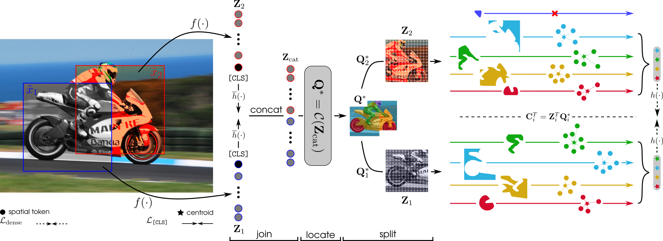
Figure 2: Overview of CrOC. The augmented views, $\tilde{\bm{x}}_{1}$ and $\tilde{\bm{x}}_{2}$, are processed independently by a ViT encoder $f$. The joint representation, $\mathbf{Z}_{\text{cat}}$, of the two image views, is obtained by concatenation along the token axis and serves as input to the clustering algorithm, $\mathcal{C}$, to locate the objects. The joint clustering assignments, $\mathbf{Q}^{*}$, are split view-wise and used to compute the corresponding centroids. A self-distillation loss enforces consistency between pairs of related centroids via a projection head $h$.

3.1 Overview

This paper tackles the problem of learning dense visual representations from unlabeled scene-centric data. Recent efforts using a self-supervised multi-view consistency paradigm to address this problem rely on a two steps procedure: i) locate the objects in each image view and ii) link the related objects from one image view to the other. We now discuss how CrOC elegantly palliates the limitations evoked in sections 1 and 2.

We observe that most of the difficulties arise because the locate-link strategy treats the two image views independently. In contrast, both views stem from the same image, and their representations lie in the same space. The former observation offers the possibility to benefit from the coordinates of the cropped image regions as a cue for the locate step, while the latter indicates that some operations could be performed conjointly. Consequently, we propose to depart from the typical strategy and introduce a novel paradigm dubbed join-locate-split, described below:

Join. The two augmented image views, $\tilde{\bm{x}}_{1}$ and $\tilde{\bm{x}}_{2}$, are processed by a ViT [12] encoder $f$ yielding the dense visual representations $\mathbf{Z}_{\{1,2\}}\in\mathbb{R}^{N\times d}$, where $N$ and $d$ denote the number of spatial tokens and feature dimension, respectively. The dense visual representations are then concatenated along the token axis to obtain the joint representation, $\mathbf{Z}_{\text{cat}}\in\mathbb{R}^{2N\times d}$.

Locate. The objective is to find semantically coherent clusters of tokens in the joint representation space. As the quality of the input representation improves, we expect the found clusters to represent the different objects or object parts illustrated in the image. The joint representation is fed to the clustering algorithm $\mathcal{C}$, which outputs the joint clustering assignments, $\mathbf{Q}^{*}\in\mathbb{R}^{2N\times K}$. The soft assignments matrix $\mathbf{Q}^{*}$ models the probability of each of the $2N$ tokens to belong to one of the $K$ clusters found in the joint space.

Split. By splitting $\mathbf{Q}^{*}$ in two along the first dimension, the assignment matrix of each view, namely $\mathbf{Q}^{*}_{\{1,2\}}\in\mathbb{R}^{N\times K}$ are obtained. One can observe that the link operation is provided for free and that it is trivial to discard any cluster that does not span across the two views.

Given the view-wise assignments $\mathbf{Q}^{*}_{\{1,2\}}$, and the corresponding dense representations $\mathbf{Z}_{\{1,2\}}$, $K$ object/cluster-level representations can be obtained for each view:

$$\begin{split}\mathbf{C}^{\top}_{1}=\mathbf{Z}^{\top}_{1}\mathbf{Q}^{*}_{1}\end{split}$$ (1)

$\mathbf{C}$ denotes the centroids. Analogously to the image-level consistency objective, one can enforce similarity constraints between pairs of centroids.

3.2 Dense self-distillation

This section details the integration of the join-locate-split strategy (Sec. 3.1) in a self-distillation scheme. Our self-distillation approach relies on a teacher-student pair of Siamese networks, $g_{t}$ and $g_{s}$, each composed of an encoder $f_{\{t,s\}}$ and a projection head $h_{\{t,s\}}$. Given the input image $\bm{x}\in\mathbb{R}^{C\times H\times W}$, two augmented views $\tilde{\bm{x}}_{1}$ and $\tilde{\bm{x}}_{2}$ are obtained using random augmentations. Both augmented views are independently passed through the teacher and student encoders, yielding the spatial representations $\mathbf{Z}_{t,\{1,2\}}$ and $\mathbf{Z}_{s,\{1,2\}}$, respectively. The teacher model’s representations are concatenated (join) and fed to the clustering algorithm (Sec. 3.3) to obtain the assignment matrix $\mathbf{Q}^{*}$ (locate), which is assumed to be already filtered of any column corresponding to an object/cluster represented in only one of the two views (cf. Sec. 3.3.1). The assignment matrix is split view-wise to get $\mathbf{Q}^{*}_{\{1,2\}}$ and to compute the teacher and student centroids of each view:

$$\begin{split}\mathbf{C}^{\top}_{\{t,s\},\{1,2\}}&=\mathbf{Z}^{\top}_{\{t,s\},\{1,2\}}\mathbf{Q}^{*}_{\{1,2\}}\\ \end{split}$$ (2)

The final step is to feed the teacher and student centroids, $\mathbf{C}_{t}$ and $\mathbf{C}_{s}$, to the corresponding projection heads, $h_{t}$ and $h_{s}$, which output probability distributions over $L$ dimensions denoted by $\mathbf{P}_{t}$ and $\mathbf{P}_{s}$, respectively. The probabilities of the teacher and student models are obtained by normalizing their projection heads’ outputs with a softmax scaled by temperatures $\tau_{t}$ and $\tau_{s}$:

$$\begin{split}\mathbf{P}_{t,\{1,2\}}&=\underset{L}{\texttt{softmax}}\left(h_{t}(\mathbf{C}_{t,\{1,2\}})/\tau_{t}\right)\\ \mathbf{P}_{s,\{1,2\}}&=\underset{L}{\texttt{softmax}}\left(h_{s}(\mathbf{C}_{s,\{1,2\}})/\tau_{s}\right)\\ \end{split}$$ (3)

The dense self-distillation objective $\mathcal{L}_{\text{dense}}$ enforces cross-view consistency of the teacher and student model projections using the cross-entropy loss:

$$\mathcal{L}_{\text{dense}}=\frac{1}{2}\left(H(\mathbf{P}_{t,1},\mathbf{P}_{s,2})+H(\mathbf{P}_{t,2},\mathbf{P}_{s,1})\right)$$ (4)

where $H(\mathbf{A},\mathbf{B})=-\frac{1}{K}\sum_{k=1}^{K}\sum_{l=1}^{L}\mathbf{A}_{kl}\log(\mathbf{B}_{kl})$ computed by averaging over all clusters.

For the dense self-distillation loss to be meaningful, the clustering assignments of spatial tokens corresponding to similar objects must be semantically coherent, which requires good-quality representations. To address this issue, we additionally apply a global representation loss by feeding the image-level representations to a dedicated projection head, $\mkern 1.5mu\overline{\mkern-1.5muh\mkern-1.5mu}\mkern 1.5mu$, to obtain the $\mkern 1.5mu\overline{\mkern-1.5muL\mkern-1.5mu}\mkern 1.5mu$-dimensional distributions:

$$\begin{split}\bm{p}_{t,\{1,2\}}&=\underset{\mkern 1.5mu\overline{\mkern-1.5muL\mkern-1.5mu}\mkern 1.5mu}{\texttt{softmax}}\left(\mkern 1.5mu\overline{\mkern-1.5muh\mkern-1.5mu}\mkern 1.5mu_{t}(\bar{\bm{z}}_{t,\{1,2\}}/\mkern 1.5mu\overline{\mkern-1.5mu\tau\mkern-1.5mu}\mkern 1.5mu_{t})\right)\\ \bm{p}_{s,\{1,2\}}&=\underset{\mkern 1.5mu\overline{\mkern-1.5muL\mkern-1.5mu}\mkern 1.5mu}{\texttt{softmax}}\left(\mkern 1.5mu\overline{\mkern-1.5muh\mkern-1.5mu}\mkern 1.5mu_{s}(\bar{\bm{z}}_{s,\{1,2\}}/\mkern 1.5mu\overline{\mkern-1.5mu\tau\mkern-1.5mu}\mkern 1.5mu_{s})\right)\end{split}$$ (5)

The sharpness of the output distribution for teacher and student models is controlled by the temperature parameters $\mkern 1.5mu\overline{\mkern-1.5mu\tau\mkern-1.5mu}\mkern 1.5mu_{t}$ and $\mkern 1.5mu\overline{\mkern-1.5mu\tau\mkern-1.5mu}\mkern 1.5mu_{s}$, respectively, and $\bar{\bm{z}}_{\{t,s\}}$ denotes the image-level representations of the teacher and student models. Hence the global representation loss $\mathcal{L}_{\text{glob}}$ is computed as follows:

$$\mathcal{L}_{\text{glob}}=\frac{1}{2}\left(H(\bm{p}_{t,1},\bm{p}_{s,2})+H(\bm{p}_{t,2},\bm{p}_{s,1})\right)$$ (6)

where $H(\mathbf{a},\mathbf{b})=-\sum_{l=1}^{\mkern 1.5mu\overline{\mkern-1.5muL\mkern-1.5mu}\mkern 1.5mu}\mathbf{a}_{l}\log(\mathbf{b}_{l})$. Therefore, the overall loss function used for the training of CrOC is:

$$\mathcal{L}=\alpha\mathcal{L}_{\text{dense}}+\mathcal{L}_{\text{glob}}$$ (7)

where $\alpha$ denotes a hyperparameter to balance the loss terms. We set $\alpha=1.0$ for all experiments without the need for hyperparameter tuning.

3.3 Where are the objects in the image?

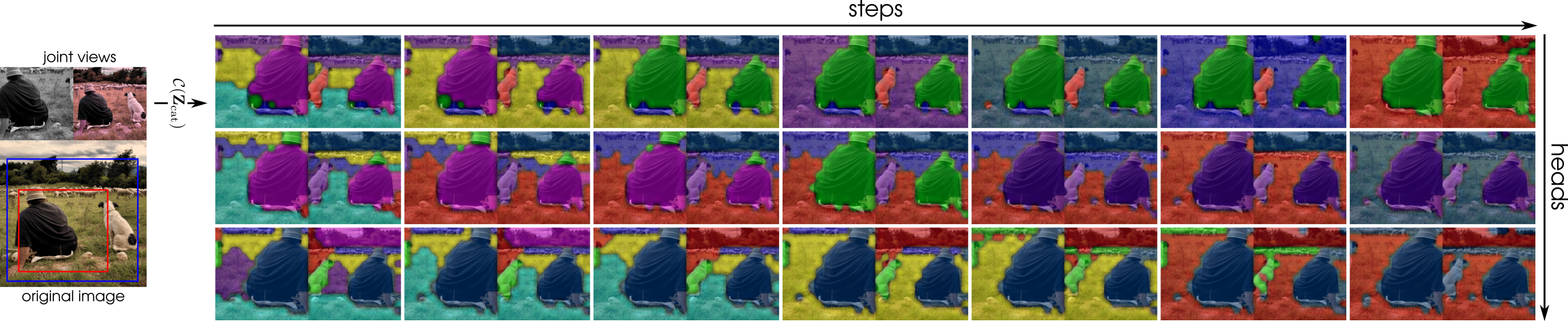
Figure 3: Representation of the iterative clustering algorithm in the joint space. The algorithm is initialized with a fixed number of centroids that are iteratively merged until only two remain. The ideal number of centroids is determined a posteriori. The procedure’s last seven steps (columns) are represented for three different heads of a ViT-S/16 pre-trained with CrOC.

So far, we assumed that there existed an algorithm able to assign a set of input data points to an undetermined number of clusters. This section covers the details of this algorithm.

The online optimization objective for computing the clusters and corresponding assignments relies on an optimal transport formulation and the Sinkhorn-Knopp algorithm [10]. This choice is motivated by i) its efficiency, ii) the ease of incorporating external knowledge (Sec. 3.3.2), and iii) it returns a measure of the clustering quality, which can be used to infer the optimal number of clusters $K$ for a given image. The last point is of utmost importance as it allows us to devise a ad-hoc selection criterion for $K$. Indeed, the iterative procedure progressively merges the centroids until only two remain, i.e., background/foreground (see Fig. 3). The number of centroids $K$ is selected a posteriori and independently for each image in the batch.

More formally, let’s consider a ViT encoder $f$ fed with a positive pair of augmented views, $\tilde{\bm{x}}_{1}$ and $\tilde{\bm{x}}_{2}$, and yielding the corresponding representations, $\mathbf{Z}_{1}$ and $\mathbf{Z}_{2}$. The clustering is performed on the joint representation, $\mathbf{Z}_{\text{cat}}\in\mathbb{R}^{2N\times d}$ obtained from the concatenation of $\mathbf{Z}_{1}$ and $\mathbf{Z}_{2}$ along the token axis. The procedure starts by sampling $K_{\text{start}}$ of the $2N$ tokens, which serve as initialization for the centroids, $\mathbf{C}\in\mathbb{R}^{K_{\text{start}}\times d}$:

$$\mathbf{C}=\mathbf{Y}^{\top}\mathbf{Z}_{\text{cat}}$$ (8)

where $\mathbf{Y}\in\{0,1\}^{2N\times K_{\text{start}}}$ is a matrix of column one-hot vectors indicating the position of the $K_{\text{start}}$ tokens used to initialize the centroids. The sampling is based on the attention map of the [CLS] token, which highlights the patches proportionally to their contribution to the image-level representation. The cost of assigning a token to a given centroid should reflect their similarity, hence:

$$\mathbf{T}^{\text{(sem)}}=-\mathbf{Z}_{\text{cat}}\mathbf{C}^{\top}$$ (9)

where $\mathbf{T}^{\text{(sem)}}\in\mathbb{R}^{2N\times K}$ denotes the cost matrix of the assignments. A handy property of the selected clustering algorithm is that it offers the possibility to scale the importance of the tokens and centroids based on external knowledge injected using a token distribution $\mathbf{r}$ and a centroid distributions $\mathbf{c}$. Here, the attention map of the [CLS] token is used as the token distribution due to its ability to highlight the sensible semantic regions of the image [6]. Along the same line, the centroids distribution is defined as:

$$\mathbf{c}=\texttt{softmax}(\mathbf{Y}^{\top}\mathbf{r})$$ (10)

Given the cost matrix, $\mathbf{T}^{\text{(sem)}}$, and the two marginals, $\mathbf{r}$ and $\mathbf{c}$, the Sinkhorn-Knopp clustering produces the assignment matrix $\mathbf{Q}^{*}$:

$$\mathbf{Q}^{*}=\underset{\mathbf{Q}\in\mathcal{U}(\mathbf{r},\mathbf{c})}{\arg\min}<\mathbf{Q},\mathbf{T}^{\text{(sem)}}>-\frac{1}{\lambda}H(\mathbf{Q})$$ (11)

where $<\cdot,\cdot>$ denotes the entry-wise product followed by a sum reduction. The second term is a regularization of the entropy of the assignments, i.e., it controls the sharpness of the clustering. $\mathcal{U}(\mathbf{r},\mathbf{c})$ is the transportation polytope, i.e., the set of valid assignments defined as:

$$\mathcal{U}(\mathbf{r},\mathbf{c})=\{\mathbf{Q}\in\mathbb{R}^{2N\times K}_{+}\>|\>\mathbf{Q}\mathbf{1}_{K}=\mathbf{r},\mathbf{Q}^{\top}\mathbf{1}_{2N}=\mathbf{c}\}$$ (12)

Additionally, the transportation cost $d_{\text{c}}$ measures the cost of assigning the tokens to the different centroids and can therefore be interpreted as the quality of the clustering, i.e., the ability to find a representative centroid for each token.

$$d_{\text{c}}=\><\mathbf{Q}^{*},\mathbf{T}^{\text{(sem)}}>$$ (13)

The centroids are updated after each step ($\mathbf{C}^{\top}=\mathbf{Z}^{\top}\mathbf{Q}^{*}$), and the two centroids, $(i^{*},j^{*})$, having the highest cosine similarity, are merged:

$$\mathbf{C},\mathbf{Y}\leftarrow\texttt{merge}(\mathbf{C},\mathbf{Y},i^{*},j^{*})$$ (14)

where merge denotes the merging operator; the merging procedure averages the selected columns of $\mathbf{Y}$ and the corresponding rows of $\mathbf{C}$; in both cases, obsolete columns/rows are simply removed from the matrices. Before reiterating through the clustering algorithm, the matrix cost, $\mathbf{T}^{\text{(sem)}}$, and centroid distribution, $\mathbf{c}$, are updated using Eq. 9 and Eq. 10, respectively. The whole procedure is repeated until only two centroids remain. By comparing the transportation cost $d_{\text{c}}$ incurred at each step (from $K_{\text{start}}$ to 2), one can select a posteriori the optimal number of centroids and the corresponding assignment $\mathbf{Q}^{*}$ for each image independently based on the $\mathbf{Q}^{*}$ that minimizes $d_{\text{c}}$. The procedure’s final step consists of the row-wise normalization of the assignments and the pruning of clusters (cf. Sec. 3.3.1).

3.3.1 Cluster pruning

An important property of CrOC is that it allows to easily discard clusters corresponding to content that is not shared across the two views (e.g., purple cluster corresponding to the helmet in Fig. 2). To that end, we first compute the hard version of the assignments (each token is assigned to precisely one centroid):

$$\mathbf{M}_{n,k}=\mathds{1}_{k=\underset{j}{\text{argmax}}\left\{\mathbf{Q}^{*}_{nj}\right\}}$$ (15)

The hard assignments are split view-wise to obtain $\mathbf{M}_{1}$ and $\mathbf{M}_{2}$, and we introduce the sets $\mathcal{S}_{1}$ and $\mathcal{S}_{2}$, which store indices of the zero columns of $\mathbf{M}_{1}$, and $\mathbf{M}_{2}$, respectively. Therefore, any column of $\mathbf{Q}^{*}_{\{1,2\}}$ and $\mathbf{M}_{\{1,2\}}$, whose index is in $\mathcal{S}=\mathcal{S}_{1}\cup\mathcal{S}_{2}$, is filtered out:

$$\mathbf{Q}_{\{1,2\}}^{*},\mathbf{M}_{\{1,2\}}\leftarrow\texttt{filter}(\mathbf{Q}_{\{1,2\}}^{*},\mathbf{M}_{\{1,2\}},\mathcal{S})$$ (16)

where filter denotes the filtering operator, which drops the indexed columns of the input matrices.

3.3.2 Positional cues

In Sec. 3.2, we mention the need for an image-level self-distillation loss to break the interdependence between the features’ quality and the correctness of the enforced dense loss. Along the same line, positional cues can be leveraged to guide the clustering operation, such that spatially coherent clusters can be obtained even when the features do not fully capture the semantics of the underlying data. Indeed, it appears natural to bias the clustering in favor of matching together tokens resulting from the same region in the original image. To that end, a positional constraint is added to the matrix transportation cost $\mathbf{T}^{\text{(sem)}}$, which is modified to incorporate this desired property.

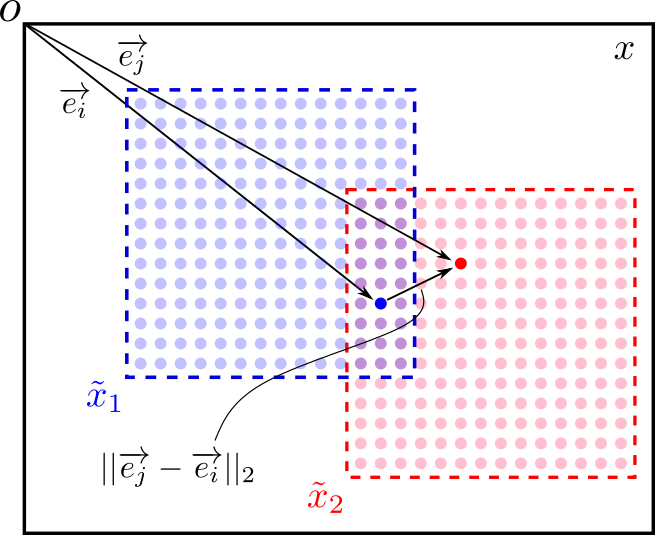
Figure 4: The positional cues use the top-left corner of the original image as a reference point, such that the position coordinates of each view lie in the same space and can be used to guide the clustering algorithm.

We start by observing that the augmented views, $\tilde{\bm{x}}_{\{1,2\}}$, result from the composition and use of a set of geometric and photometric transformations on the original image $\bm{x}$. We propose to extract the coordinates of the patches in each view with respect to the original image referential (cf. Fig. 4). More precisely, we generate the tensors, $\mathbf{E}_{\{1,2\}}\in\mathbb{R}^{N\times 2}$, which store the 2D coordinates of each patch in the two views. The coordinates are first concatenated along the patch/token axis to obtain $\mathbf{E}_{\text{cat}}\in\mathbb{R}^{2N\times 2}$, and the positions of the centroids, $\mathbf{E}_{\text{cen}}\in\mathbb{R}^{K_{\text{start}}\times 2}$, are computed as in Eq. 8 ($\mathbf{E}_{\text{cen}}=\mathbf{Y}^{\top}\mathbf{E}_{\text{cat}}$). The entries of the positional transportation cost $\mathbf{T}^{\text{(pos)}}\in\mathbb{R}^{2N\times K_{\text{start}}}$ are computed as follows:

$$\mathbf{T}^{\text{(pos)}}_{ij}=\frac{1}{S}||\mathbf{e}^{\text{(cat)}}_{i}-\mathbf{e}^{\text{(cen)}}_{j}||_{2}$$ (17)

where $S$ is a normalization constant that ensures that the entries of the positional transportation cost are in $[0,1]$. After incorporation of the positional bias, the total matrix transportation cost is defined as follows:

$$\mathbf{T}^{\text{(tot)}}=\mathbf{T}^{\text{(sem)}}+\lambda_{\text{pos}}\mathbf{T}^{\text{(pos)}}$$ (18)

The scalar weight $\lambda_{\text{pos}}$ regulates the importance of the positional cues. As detailed in Sec. 3.3, the clustering algorithm relies on the iterative merging of the centroids; hence their respective position must also be merged reciprocally, i.e., by averaging (cf. Eq. 14).

3.3.3 Multiple clustering assignments using MSA

In this section, we detail a mechanism to obtain multiple complementary clustering assignments $\mathbf{Q}^{*}$ per image. This mechanism relies on the multi-head self-attention (MSA) module inherent to the transformer architecture.

Arguably, the main ingredient behind the transformer architecture’s success is the self-attention module. Indeed, i) it allows capturing of long-range inter-dependencies between the patches that constitute the image, and ii) it endows the local representations with global or contextual information. Formally, the multi-head attention operation of the $l^{th}$ transformer block is expressed as:

$$\begin{split}\texttt{multi}&\texttt{-head}\left(\mathbf{Z}^{(l-1)}\right)\\ &=\texttt{concat}\left(\text{head}_{1},...,\text{head}_{n_{h}}\right)\mathbf{W}^{o}\end{split}$$ (19)

where $\mathbf{W}^{o}\in\mathbb{R}^{d\times d}$ is a learnable projection weight, and $\text{head}_{i}$, for $i=1,\cdots,n_{h}$, denotes a single attention head:

$$\text{head}_{i} =\texttt{attention}\left(\mathbf{Z}^{(l-1)},\mathbf{W}^{\{q,k,v\}}_{i}\right)$$ (20)

$$=\texttt{softmax}\left(\frac{\mathbf{Z}^{(l-1)}\mathbf{W}_{i}^{q}\left(\mathbf{Z}^{(l-1)}\mathbf{W}_{i}^{k}\right)^{\top}}{\sqrt{D}}\right)\mathbf{Z}^{(l-1)}\mathbf{W}_{i}^{v}$$

where $\mathbf{W}_{i}^{\{q,k,v\}}\in\mathbb{R}^{d\times d/n_{h}}$ denotes head-specific learnable projection weights. Following the same reasoning that motivates the use of multiple heads, i.e., the inter-patches relationship is not unique, we use as many clustering assignments as there are heads in the MSA module. In practice, it turns out to be as simple as independently feeding each attention head’s dense representation to the clustering algorithm:

$$\mathbf{Q}^{i}=\mathcal{C}\left(\mathbf{Z}^{(B-2)}\mathbf{W}_{i}^{k}\right)$$ (21)

where $B$ is the number of transformer blocks in the model. Note that only one of the keys/queries/values representation is used (here exemplified with the keys). Consequently, the final assignment matrix $\mathbf{Q}^{*}$ results from the concatenation of the head-wise assignments $\mathbf{Q}^{i}$ along the centroid dimension. Up to pruning (Sec. 3.3.1), the effective number of centroids is $n_{h}$ times higher. Even though the clusters overlap, we do not enforce contradictory objectives as i) the consistency is enforced pair-wise (from one centroid in the first view to the corresponding one in the second view) and ii) in the framework of self-distillation there are no negative pairs.

4 Experiments

4.1 Implementations details

Pre-training datasets. Our models are pre-trained on two uncurated and scene-centric datasets, namely COCO (train2017, $\sim$118k images) and COCO+ (unlabeled2017 + train2017, $\sim$241k images). We further explore the possibility of using CrOC in an object-centric scenario and therefore adopt ImageNet [11] as a pre-training dataset ($\sim 10\times$ more images and $\sim 4\times$ fewer objects/image).

Network architecture. We use a ViT-small (ViT-S/16) as the backbone $f$. This choice is in line with its adoption in concurrent methods and for its comparability [6, 51, 49] with the ResNet50, which is the backbone of the remaining baselines. The architecture of the projection heads is identical to that of [6]. Notably, the image-level and centroids-level heads, $\mkern 1.5mu\overline{\mkern-1.5muh\mkern-1.5mu}\mkern 1.5mu$ and $h$, share their weights except for the last layer, which has output dimensions, $\mkern 1.5mu\overline{\mkern-1.5muL\mkern-1.5mu}\mkern 1.5mu=65,536$ and $L=8,192$, respectively.

Optimization. CrOC is trained for 300 epochs on COCO and COCO+ under an identical optimization scheme. A batch size of 256, distributed over 2 Tesla V100 GPUs is used. The pre-training on ImageNet uses a batch size of 1024, distributed over 4 AMD MI250X GPUs. The remaining optimization setting is identical to that of DINO [6].

Hyperparameters. The same weight is given to the dense and global loss, i.e., $\alpha=1$. We use $\lambda=20$ for the regularization term of the transportation objective. The dense and global projection heads use the same temperature parameters, namely $\mkern 1.5mu\overline{\mkern-1.5mu\tau\mkern-1.5mu}\mkern 1.5mu_{s}=\tau_{s}=0.1$ and $\mkern 1.5mu\overline{\mkern-1.5mu\tau\mkern-1.5mu}\mkern 1.5mu_{t}=\tau_{t}=0.07$ (see Eqs. 3 & 5). Generally, any hyper-parameter common to DINO uses its recommended value. The results of section 4.3 which use COCO or COCO+ as pre-training datasets are obtained with $\lambda_{\text{pos}}=4$, $K_{\text{start}}=12$ and the values tokens as parameters of the clustering algorithm. For ImageNet, we only report results with $\lambda_{\text{pos}}=3$, $K_{\text{start}}=12$ and the keys tokens. These values correspond to the default setting of the grid search performed on COCO (see Sec. 4.4).

4.2 Evaluation protocols

We opt for dense evaluation downstream tasks, which require as little manual intervention as possible, such that the reported results truly reflect the quality of the features. Details of the implementations and datasets are available in Appendix C.

Transfer learning via linear segmentation. The linear separability of the learned spatial features is evaluated by training a linear layer on top of the frozen features of the pre-trained encoder. The linear layer implements a mapping from the embedding space to the label space and is trained to minimize the cross-entropy loss. We report the mean Intersection over Union (mIoU) of the resulting segmentation maps on four different datasets, namely, PVOC12 [13], COCO-Things, COCO-Stuff [29] and ADE20K [50].

Transfer learning via unsupervised segmentation. We evaluate the ability of the methods to produce spatial features that can be grouped into coherent clusters. We perform K-Means clustering on the spatial features of every image in a given dataset with as many centroids as there are classes in the dataset. Subsequently, a label is assigned to each cluster via Hungarian matching [25]. We report the mean Intersection over Union (mIoU) of the resulting segmentation maps on three different datasets, namely PVOC12 [13], COCO-Things, and COCO-Stuff [29].

Semi-supervised video object segmentation. We assess our method’s generalizability for semi-supervised video object segmentation on the DAVIS’17 benchmark. The purpose of this experiment is to evaluate the spatiotemporal consistency of the learned features. First, the features of each frame in a given video are independently obtained; secondly, a nearest-neighbor approach is used to propagate (from one frame to the next) the ground-truth labels of the first frame (see results in Appendix D).

4.3 Segmentation results

In Tables 1 and 2, we report mIoU results on the linear segmentation task. When pre-trained on COCO, CrOC exceeds concurrent methods using COCO(+) as pre-training datasets, even though ORL and BYOL use a longer training protocol (800 epochs). With a pre-training on COCO+, CrOC outperforms all other methods, except $\text{CP}^{2}$ [39], on every evaluation dataset, despite their usage of ImageNet and their finetuning on one of the target datasets (PVOC12). Noteworthy that $\text{CP}^{2}$ is initialized with a pre-trained model and cannot be trained from scratch. Pre-training on a larger and object-centric dataset appears to be highly beneficial in that setting.

Table 1: Transfer results of linear segmentation task. A linear layer is trained on top of the frozen spatial features. The mIoU scores are reported on the PVOC12 [13], COCO-Things (CC-Th.), and COCO-Stuff (CC-St.) [29]. The pre-training dataset is either of ImageNet (IN) [11], COCO (CC), or COCO+ (CC+).

Method	Model / Dataset	PVOC12	CC-Th.	CC-St.	Avg.
Global features
BYOL [15]	ResNet50 / CC+	38.7	50.4	39.8	43.0
DINO [6]	ViT-S/16 / CC	47.2	47.1	46.2	46.8
Local features
ORL [47]	ResNet50 / CC+	45.2	55.6	45.6	48.8
DenseCL [41]	ResNet50 / IN	57.9	60.4	47.5	55.3
SoCo [43]	ResNet50 / IN	54.0	56.8	44.2	51.7
ReSim [45]	ResNet50 / IN	55.1	57.7	46.5	53.1
PixPro [48]	ResNet50 / IN	57.1	54.7	45.9	52.6
VICRegL [2]	ResNet50 / IN	58.9	58.7	48.2	55.3
MAE [18]	ViT-S/16 / CC	31.7	35.1	39.6	35.5
$\text{CP}^{2}$ [39]	ViT-S/16 / IN+PVOC12	63.1	59.4	46.5	56.3
Ours
cyan!20 CrOC	ViT-S/16 / CC	54.5	55.6	49.7	53.3
cyan!20 CrOC	ViT-S/16 / CC+	60.6	62.7	51.7	58.3
cyan!20 CrOC	ViT-S/16 / IN	70.6	66.1	52.6	63.1

In Table 3, the results for the unsupervised segmentation task are reported. As for linear segmentation experiments, CrOC is already competitive with only a pre-training on the COCO dataset and surpasses all competing methods except DenseCL [41].

Table 2: Transfer results of linear segmentation task. A linear layer is trained on top of the frozen spatial features. The mIoU scores are reported for ADE20k [50]. The pre-training dataset is either ImageNet [11], COCO, or COCO+.

Method	Model	Dataset	Epochs	mIoU
Global features
DINO [6]	ViT-S/16	COCO	300	18.5
DINO [6]	ViT-S/16	ImageNet	800	26.8
Local features
DenseCL [41]	ResNet50	ImageNet	200	24.3
VICRegL [2]	ResNet50	ImageNet	300	23.7
$\text{CP}^{2}$ [39]	ViT-S/16	ImageNet+PVOC12	320	25.4
Ours
cyan!20 CrOC	ViT-S/16	COCO	300	23.2
cyan!20 CrOC	ViT-S/16	COCO+	300	27.0
cyan!20 CrOC	ViT-S/16	ImageNet	300	28.4

The largest improvements are observed on the COCO-Stuff dataset; this is unsurprising as this dataset contains semantic labels such as water, ground, or sky, which correspond to regions that are typically overlooked by other methods, but on which CrOC puts a significant emphasis. The model pre-trained on ImageNet appears to perform poorly on that task, which is surprising considering the excellent results depicted in Table 1 on the exact same datasets. This might hint that using evaluations that are not adjustable to each baseline is sub-optimal. Overall we observe that producing features that can be clustered class-wise without labels remains an open challenge.

Table 3: Transfer results of unsupervised segmentation task. The frozen spatial features of each image in a given dataset are clustered into as many clusters as there are classes in the dataset. The Hungarian matching algorithm is used to label the clusters. The mIoU scores are reported on PVOC12 [13], COCO-Things (CC-Th.) and COCO-Stuff (CC-St.) [29]. The pre-training dataset is either of ImageNet (IN) [11], COCO (CC), or COCO+ (CC+).

Method	Model / Dataset	PVOC12	CC-Th.	CC-St.	Avg.
Global features
BYOL [15]	ResNet50 / CC+	13.6	9.4	8.9	10.6
DINO [6]	ViT-S/16 / CC	5.2	9.4	14.0	9.5
Local features
ORL [47]	ResNet50 / CC+	11.9	12.0	13.7	12.5
DenseCL [41]	ResNet50 / IN	18.0	19.2	16.9	18.0
SoCo [43]	ResNet50 / IN	15.1	16.3	18.9	16.8
ReSim [45]	ResNet50 / IN	17.1	15.9	16.6	16.5
PixPro [48]	ResNet50 / IN	9.5	15.2	12.4	12.4
VICRegL [2]	ResNet50 / IN	13.9	11.2	16.0	13.7
MAE [18]	ViT-S/16 / CC	3.3	7.5	13.6	8.1
$\text{CP}^{2}$ [39]	ViT-S/16 / IN	9.5	12.9	13.6	12.0
Ours
cyan!20 CrOC	ViT-S/16 / CC	16.1	17.2	20.0	17.8
cyan!20 CrOC	ViT-S/16 / CC+	20.6	17.1	21.9	19.9
cyan!20 CrOC	ViT-S/16 / IN	3.8	5.4	6.6	5.3

4.4 Ablation study

We scrutinize the roles played by different components of CrOC. Unless otherwise stated, $\lambda_{\text{pos}}=3$, $K_{\text{start}}=12$ and the keys tokens are used for the ablations. Rows corresponding to the chosen setting are highlighted.

Weight of the positional cues $\lambda_{\text{pos}}$. The first element that is ablated is the contribution of the positional bias to the overall performance. In Table 4, we observe that an increased positional bias leads to improved performance on the unsupervised segmentation task, but a slightly worsened one on the linear segmentation task.

Table 4: Ablation: positional cues weight $\lambda_{\text{pos}}$. We report the mIoU scores for linear and unsupervised segmentation tasks.

	PVOC12			COCO-Things			COCO-Stuff
$\lambda_{\text{pos}}$	Unsupervised	Linear		Unsupervised	Linear		Unsupervised	Linear
0	3.4	52.2		6.8	53.8		6.3	48.9
1	4.0	55.8		6.8	56.6		8.3	50.3
2	6.9	56.7		7.8	58.0		13.3	50.4
3	15.7	56.5		12.1	56.5		17.9	50.2
cyan!20 4	16.4	55.0		17.0	56.9		20.9	50.4
$\infty$	2.3	55.9		5.4	57.2		5.5	50.1

Table 5: Ablation: initial number of centroids $K_{\text{start}}$. We report the mIoU scores for both the linear and unsupervised segmentation downstream tasks.

	PVOC12			COCO-Things			COCO-Stuff
$K_{\text{start}}$	Unsupervised	Linear		Unsupervised	Linear		Unsupervised	Linear
4	5.3	48.0		8.3	48.7		12.6	47.5
8	15.8	54.8		17.6	56.5		23.4	49.8
cyan!20 12	15.7	56.5		12.1	56.5		17.9	50.2
16	10.9	56.9		8.0	58.0		14.2	50.5

Number of initial centroids $K_{\text{start}}$. As can be seen in Table 5, the linear segmentation scores monotonically increase with the number of initial centroids, whereas for unsupervised segmentation, there seems to be a middle ground.

Type of clustering tokens. Table 6 shows that the choice of spatial tokens plays a determinant role in the downstream results and that the multi-clustering approach (Sec. 3.3.3) can yield a significant boost in performance compared to the case when the clustering uses last spatial tokens $\mathbf{Z}^{(B-1)}$ (last).

Table 6: Ablation: type of tokens used for the clustering. We evaluate the impact of using either of the keys, values, or queries tokens of the last transformer block. We report the mIoU scores for both the linear and unsupervised segmentation downstream tasks.

	PVOC12			COCO-Things			COCO-Stuff
Tokens	Unsupervised	Linear		Unsupervised	Linear		Unsupervised	Linear
last	11.2	52.6		12.7	54.6		16.0	49.1
queries	8.3	55.1		7.6	56.5		11.9	49.8
keys	15.7	56.5		12.1	56.5		17.9	50.2
cyan!20 values	16.5	55.2		16.0	55.8		21.5	49.5

5 Conclusion

We introduced CrOC; a novel SSL pre-training method for dense downstream tasks. CrOC does not resort to using hand-crafted priors and the online clustering algorithm generates pseudo labels for both views in a single and united step. As such, the generated segmentation masks are more coherent and avoid encouraging similarity between objects not univocally represented in both views. CrOC is thoroughly evaluated on various downstream tasks and datasets. In spite of being pre-trained on a medium size scene-centric dataset, the proposed learning paradigm is competitive or outperforms existing methods using ImageNet.

Limitation. As is the case with most dense SSL methods, CrOC is only implemented and tested with a single model.

Appendix

This Appendix provides additional details and qualitative results organized as follows. In Appendix A, we thoroughly describe the datasets used in our paper. Additional details about concurrent methods and comparison are discussed in Appendix B. A detailed description of the evaluation protocols is presented in Appendix C. Additional results on semi-supervised video segmentation are reported in Appendix D. In Appendix E, we briefly discuss the efficiency and computational overhead of CrOC. Finally, we provide examples of the clusters found on the combined views of complex scene images with the proposed online clustering algorithm in Appendix F.

Appendix A Datasets

COCO. The COCO (Microsoft Common Objects in Context) dataset [29] consists of scene-centric images spanning 91 stuff categories and 80 objects/things categories. The train2017, val2017 and test2017 splits incorporate approximately 118k, 5k and 41k images, respectively. Additionally, a set of $\sim$123k unlabeled images, unlabeled2017, can be used in conjunction with the train2017 split to obtain the so-called COCO+ training set.

COCO-Things. The COCO-Things dataset follows the implementation of [51]. This dataset is based on COCO images and the panoptic labels of [24]. More precisely, the instance-level labels are merged, and so are the 80 “things” categories, yielding the following 12 super-categories: electronic, kitchen, appliance, sports, vehicle, animal, food, furniture, person, accessory, indoor, and outdoor. As the underlying images are the same as in the COCO dataset, so are the training/validation/test splits.

COCO-Stuff. The COCO-Stuff dataset follows the implementation of [51]. The stuff annotations are those of [3]. As for COCO-Things, the 91 “stuff” categories are merged into 15 super-categories: water, structural, ceiling, sky, building, furniture-stuff, solid, wall, raw-material, plant, textile, floor, food-stuff, ground and window. This dataset follows the same training/validation/test splits as in the COCO dataset.

PVOC12. The PASCAL VOC12 (PVOC12) dataset [13] is a scene-centric dataset. The trainaug split relies on the extra annotations of [17] such that 10582 images with pixel-level labels can be used for the training phase as opposed to the 1464 segmentation masks initially available. The validation set encompasses 1449 finely annotated images. The dataset spans 20 object classes (+1 background class): person, bird, cat, cow, dog, horse, sheep, aeroplane, bicycle, boat, bus, car, motorbike, train, bottle, chair, dining table, potted plant, sofa, tv/monitor and background.

ADE20K. The ADE20K dataset [50] is a scene-centric dataset encompassing more than 20K scene-centric images and pixel-level annotations. The labels span 150 semantic categories, including “stuff” categories, e.g. sky, road, or grass, and “thing” categories, e.g. person, car, etc.

Appendix B Implementation details

B.1 Comparison with competing methods

To compare CrOC on an equal footing with concurrent methods, we evaluate all baselines using our evaluation pipeline, except for the evaluation of ResNet50 on the semi-supervised video segmentation task which are taken as is from [49]. With our implementation, the results were worse than the ones reported in [49] or [21]; hence we report their results. Furthermore, for BYOL [15], ORL [47], DenseCL [41], SoCo [43], ReSim [45], PixPro [48], VICRegL [2] and $\text{CP}^{2}$ [39], we use publicly available model checkpoints. The only two exceptions are MAE [18] and DINO [6] methods. Indeed, no public model checkpoint exists for ViT-S/16 pre-trained with MAE. Since our implementation builds upon DINO, it is important to have CrOC and DINO models trained in a similar setting for comparison purposes.

MAE. The ViT-S/16 is pre-trained under MAE framework on the COCO dataset with the following parameters:

• mask_ratio: 0.75

• weight_decay: 0.05

• base_lr: 0.00015

• min_lr: 0.0

• warmup_epochs: 40

• batch_size: 256

• epochs: 300

We use the following decoder architecture:

• decoder_embed_dim: 512

• decoder_depth: 8

• decoder_num_heads: 16

DINO. The ViT-S/16 is pre-trained under DINO framework on the COCO dataset with the following parameters:

• out_dim: 65536

• norm_last_layer: false

• warmup_teacher_temp: 0.04

• teacher_temp: 0.07

• warmup_teacher_temp_epochs: 30

• use_fp16: true

• weight_decay: 0.04

• weight_decay_end: 0.4

• clip_grad: 0

• batch_size: 256

• epochs: 300

• freeze_last_layer: 1

• lr: 0.0005

• warmup_epochs: 10

• min_lr: 1e-05

• global_crops_scale: [0.25, 1.0]

• local_crops_number: 0

• optimizer: adamw

• momentum_teacher: 0.996

• use_bn_in_head: false

• drop_path_rate: 0.1

Appendix C Evaluation protocols

For all evaluation protocols and models, the evaluation operates on the frozen features of the backbone. The projection heads, if any, are simply discarded. The output features from layer4 of ResNet50 are used in all downstream tasks. The resulting features have dimension $d=2048$, whereas the spatial tokens of a ViT-S/16 have dimension $d=384$ only. We concatenate the spatial tokens from the last $n_{b}$ transformer blocks, similar to [6], to compensate for that difference.

Transfer learning via linear segmentation. Our implementation is based on that of [38, 51]. The input images are re-scaled to $448\times 448$ pixels and fed to the frozen model. Following existing works [51], in the case of ResNet50, dilated convolutions are used in the last bottleneck layer such that the resolution of the features is identical for all models. Prior to their processing by the linear layer, the features are up-sampled with bilinear interpolation such that the predictions and the ground-truths masks have the same resolution. Unlike previous works [51, 2, 38], we use Adam [23] as an optimizer instead of SGD. Indeed, we observe that this led to significant improvements for all baselines, indicating that the reported results were obtained in a sub-optimal regime and hence did not fully reflect the quality of the learned features. We report results on the PVOC12 validation set after training the linear layer on the trainaug split for 45 epochs. For the COCO-Things and COCO-Stuff, the linear layer is first trained for 10 epochs on the training set and subsequently evaluated on the validation set. Regardless of the evaluation dataset and model, we find that a learning rate lr=1e-3 works well and that the selected number of epochs is sufficient to reach convergence. Note that contrary to [51], which randomly samples 10% of the COCO-Things/-Stuff training images, we use the full set of available images to avoid introducing additional randomness in the results.

For the evaluation with ADE20K, we rely on MMSegmentation [9] and the 40k iterations schedule. We set the batch size to 16, and we report for each method the best result after trying learning rates in $\{\texttt{1e-03},\texttt{8e-04},\texttt{3e-04},\texttt{1e-04},\texttt{8e-05}\}$.

Transfer learning via unsupervised segmentation. Our implementation is based on that of [38, 51]. The input images are re-scaled to $448\times 448$ pixels and fed to the frozen model. Following existing works [51], in the case of ResNet50, dilated convolutions are used in the last bottleneck layer such that the resolution of the features is identical for all models. Similarly to [51], the ground-truth segmentation masks and features are down-/up-sampled to have the same resolution ($100\times 100$). Consequently, we ran K-Means on the spatial features of all images with as many clusters as there are classes in the dataset. A label is greedily assigned to each cluster with Hungarian matching [25]. We report the mean Intersection over Union (mIoU) score averaged over five seeds. Importantly, [51] observed that better results could be obtained by using a larger number of clusters $K$ than the number of classes in the dataset and hereby having clusters of object-parts instead of objects. Indeed, if this approach provides information on the consistency of the features within object-part clusters, it does not tell anything about the inter-object-parts relationship. For instance, the mIoU scores will reflect the ability of features corresponding to “car wheels” to be clustered together and similarly for “car body” features, but it won’t be impacted by the distance of the two clusters from one another, which is undesirable. We report results on the PVOC12, COCO-Things, and COCO-Stuff validation sets.

Semi-supervised video object segmentation. The semi-supervised video object segmentation evaluation follows the implementation of [6, 49]. We report the mean contour-based accuracy $\mathcal{F}_{m}$, mean region similarity $\mathcal{J}_{m}$ and their average $(\mathcal{J}\&\mathcal{F})_{m}$ on the 30 videos from the validation set of the DAVIS’17 [34]. The following parameters are used:

• n_last_frames: 7

• size_mask_neighborhood: 12

• topk: 5

Appendix D Semi-supervised video segmentation results

Table A1: Semi-supervised video object segmentation task. The frozen spatial features are evaluated on the video segmentation task by nearest neighbor propagation DAVIS’17 challenge. The mean region similarity $\mathcal{J}_{m}$, mean contour-based accuracy $\mathcal{F}_{m}$, and their average ($\mathcal{J}\&\mathcal{F})_{m}$ are reported. $\dagger$ indicates results taken from [49].

Method	Model	Dataset	($\mathcal{J}\&\mathcal{F})_{m}$	$\mathcal{J}_{m}$	$\mathcal{F}_{m}$
Global features
DINO [6]	ViT-S/16	COCO	57.1	55.3	58.9
Local features
$\text{DenseCL}^{\dagger}$ [41]	ResNet50	ImageNet	50.7	52.6	48.9
$\text{ReSim}^{\dagger}$ [45]	ResNet50	ImageNet	49.3	51.2	47.3
$\text{DetCo}^{\dagger}$ [46]	ResNet50	ImageNet	56.7	57.0	56.4
ODIN [21]	ResNet50	ImageNet	54.1	54.3	53.9
MAE [18]	ViT-S/16	COCO	48.9	47.3	50.6
$\text{CP}^{2}$ [39]	ViT-S/16	ImageNet	53.7	51.3	56.1
Ours
cyan!20 CrOC	ViT-S/16	COCO	57.4	55.7	59.1
cyan!20 CrOC	ViT-S/16	COCO+	58.4	56.5	60.2
cyan!20 CrOC	ViT-S/16	ImageNet	44.7	43.5	45.9

Good results are obtained on the semi-supervised video segmentation (Table A1), indicating the ability of CrOC to produce features consistent through time and space.

Appendix E Computational overhead

An important property of CrOC is that it generates pseudo-labels/cluster assignments online. Consequently, this step must be efficient. In Table A2, we verify that the operations inherent to the clustering step amount to less than $10\%$ of the total time of the CrOC pipeline.

Table A2: The runtime of the main operations in CrOC for a batch size of 256 samples distributed over 2 Tesla V100. CrOC-specific operations are highlighted.

operation	absolute time [ms]	relative time [%]
$f_{t}(\cdot)+\mkern 1.5mu\overline{\mkern-1.5muh\mkern-1.5mu}\mkern 1.5mu_{t}(\cdot)$	177.8	21.1
$f_{s}(\cdot)+\mkern 1.5mu\overline{\mkern-1.5muh\mkern-1.5mu}\mkern 1.5mu_{s}(\cdot)$	183.9	21.9
cyan!20 $\mathbf{Q}^{*}=\mathcal{C}(\cdot)$	67.0	8
cyan!20 $h_{t}(\cdot)+h_{s}(\cdot)$	4.8	0.5
backprop. + EMA	408.0	48.5
total	841.5	100

Appendix F Qualitative results

The cluster assignments found by CrOC’s dedicated online clustering algorithm $\mathcal{C}$ over the combined views are depicted in Fig. A1. The model used to generate the illustrated assignments is pre-trained on the COCO+ for 300 epochs with CrOC and the following meta-parameters: $\lambda_{\text{pos}}=4$, $K_{\text{start}}=12$ and values tokens. During training, we use the same augmentations as in DINO [6]; consequently, we visualize the generated masks based on augmented views in the same manner, such that the results depicted in Fig. A1 truly reflect the consistency enforced by CrOC.

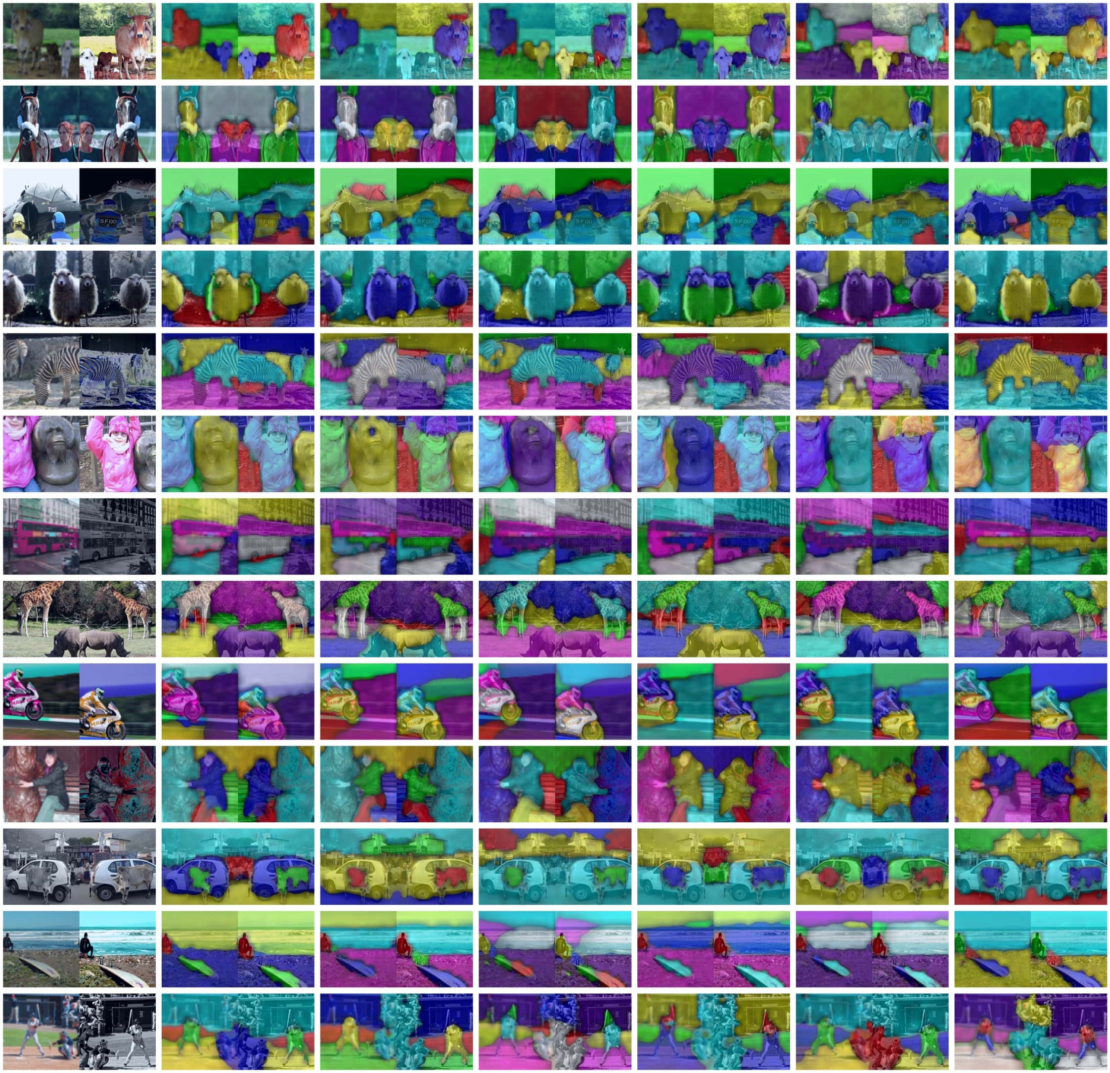
Figure A1: Illustration of the clusters found online in the space of the combined views. Rows correspond to combined views and columns to heads of the ViT. Bicubic interpolation is used to up-sample the assignments $\mathbf{Q}^{*}$ to the same resolution as the images.

References

- [1] Yuki Markus Asano, Christian Rupprecht, and Andrea Vedaldi. Self-labelling via simultaneous clustering and representation learning. arXiv preprint arXiv:1911.05371, 2019.
- [2] Adrien Bardes, Jean Ponce, and Yann LeCun. Vicregl: Self-supervised learning of local visual features. arXiv preprint arXiv:2210.01571, 2022.
- [3] Holger Caesar, Jasper Uijlings, and Vittorio Ferrari. Coco-stuff: Thing and stuff classes in context. In Proceedings of the IEEE conference on computer vision and pattern recognition, pages 1209–1218, 2018.
- [4] Mathilde Caron, Piotr Bojanowski, Armand Joulin, and Matthijs Douze. Deep clustering for unsupervised learning of visual features. In Proceedings of the European conference on computer vision (ECCV), pages 132–149, 2018.
- [5] Mathilde Caron, Ishan Misra, Julien Mairal, Priya Goyal, Piotr Bojanowski, and Armand Joulin. Unsupervised learning of visual features by contrasting cluster assignments. In Thirty-fourth Conference on Neural Information Processing Systems (NeurIPS), 2020.
- [6] Mathilde Caron, Hugo Touvron, Ishan Misra, Hervé Jégou, Julien Mairal, Piotr Bojanowski, and Armand Joulin. Emerging properties in self-supervised vision transformers. arXiv preprint arXiv:2104.14294, 2021.
- [7] Ting Chen, Simon Kornblith, Mohammad Norouzi, and Geoffrey Hinton. A simple framework for contrastive learning of visual representations. In International conference on machine learning, pages 1597–1607. PMLR, 2020.
- [8] Jang Hyun Cho, Utkarsh Mall, Kavita Bala, and Bharath Hariharan. Picie: Unsupervised semantic segmentation using invariance and equivariance in clustering. In Proceedings of the IEEE/CVF Conference on Computer Vision and Pattern Recognition, pages 16794–16804, 2021.
- [9] MMSegmentation Contributors. MMSegmentation: Openmmlab semantic segmentation toolbox and benchmark. https://github.com/open-mmlab/mmsegmentation, 2020.
- [10] Marco Cuturi. Sinkhorn distances: Lightspeed computation of optimal transport. Advances in neural information processing systems, 26:2292–2300, 2013.
- [11] Jia Deng, Wei Dong, Richard Socher, Li-Jia Li, Kai Li, and Li Fei-Fei. Imagenet: A large-scale hierarchical image database. In 2009 IEEE Conference on Computer Vision and Pattern Recognition, pages 248–255, 2009.
- [12] Alexey Dosovitskiy, Lucas Beyer, Alexander Kolesnikov, Dirk Weissenborn, Xiaohua Zhai, Thomas Unterthiner, Mostafa Dehghani, Matthias Minderer, Georg Heigold, Sylvain Gelly, et al. An image is worth 16x16 words: Transformers for image recognition at scale. arXiv preprint arXiv:2010.11929, 2020.
- [13] M. Everingham, L. Van Gool, C. K. I. Williams, J. Winn, and A. Zisserman. The PASCAL Visual Object Classes Challenge 2012 (VOC2012) Results. http://www.pascal-network.org/challenges/VOC/voc2012/workshop/index.html.
- [14] Spyros Gidaris, Praveer Singh, and Nikos Komodakis. Unsupervised representation learning by predicting image rotations. arXiv preprint arXiv:1803.07728, 2018.
- [15] Jean-Bastien Grill, Florian Strub, Florent Altché, Corentin Tallec, Pierre H Richemond, Elena Buchatskaya, Carl Doersch, Bernardo Avila Pires, Zhaohan Daniel Guo, Mohammad Gheshlaghi Azar, et al. Bootstrap your own latent: A new approach to self-supervised learning. arXiv preprint arXiv:2006.07733, 2020.
- [16] Mark Hamilton, Zhoutong Zhang, Bharath Hariharan, Noah Snavely, and William T Freeman. Unsupervised semantic segmentation by distilling feature correspondences. arXiv preprint arXiv:2203.08414, 2022.
- [17] Bharath Hariharan, Pablo Arbeláez, Lubomir Bourdev, Subhransu Maji, and Jitendra Malik. Semantic contours from inverse detectors. In 2011 international conference on computer vision, pages 991–998. IEEE, 2011.
- [18] Kaiming He, Xinlei Chen, Saining Xie, Yanghao Li, Piotr Dollár, and Ross Girshick. Masked autoencoders are scalable vision learners. arXiv preprint arXiv:2111.06377, 2021.
- [19] Kaiming He, Haoqi Fan, Yuxin Wu, Saining Xie, and Ross Girshick. Momentum contrast for unsupervised visual representation learning. In Proceedings of the IEEE/CVF Conference on Computer Vision and Pattern Recognition, pages 9729–9738, 2020.
- [20] Olivier J Hénaff, Skanda Koppula, Jean-Baptiste Alayrac, Aaron van den Oord, Oriol Vinyals, and João Carreira. Efficient visual pretraining with contrastive detection. arXiv preprint arXiv:2103.10957, 2021.
- [21] Olivier J Hénaff, Skanda Koppula, Evan Shelhamer, Daniel Zoran, Andrew Jaegle, Andrew Zisserman, João Carreira, and Relja Arandjelović. Object discovery and representation networks. arXiv preprint arXiv:2203.08777, 2022.
- [22] R Devon Hjelm, Alex Fedorov, Samuel Lavoie-Marchildon, Karan Grewal, Phil Bachman, Adam Trischler, and Yoshua Bengio. Learning deep representations by mutual information estimation and maximization. arXiv preprint arXiv:1808.06670, 2018.
- [23] Diederik P Kingma and Jimmy Ba. Adam: A method for stochastic optimization. arXiv preprint arXiv:1412.6980, 2014.
- [24] Alexander Kirillov, Kaiming He, Ross Girshick, Carsten Rother, and Piotr Dollár. Panoptic segmentation. In Proceedings of the IEEE/CVF Conference on Computer Vision and Pattern Recognition, pages 9404–9413, 2019.
- [25] Harold W Kuhn. The hungarian method for the assignment problem. Naval research logistics quarterly, 2(1-2):83–97, 1955.
- [26] Gustav Larsson, Michael Maire, and Gregory Shakhnarovich. Colorization as a proxy task for visual understanding. In Proceedings of the IEEE conference on computer vision and pattern recognition, pages 6874–6883, 2017.
- [27] Tim Lebailly and Tinne Tuytelaars. Global-local self-distillation for visual representation learning. arXiv preprint arXiv:2207.14676, 2022.
- [28] Chunyuan Li, Jianwei Yang, Pengchuan Zhang, Mei Gao, Bin Xiao, Xiyang Dai, Lu Yuan, and Jianfeng Gao. Efficient self-supervised vision transformers for representation learning. arXiv preprint arXiv:2106.09785, 2021.
- [29] Tsung-Yi Lin, Michael Maire, Serge Belongie, James Hays, Pietro Perona, Deva Ramanan, Piotr Dollár, and C Lawrence Zitnick. Microsoft coco: Common objects in context. In European conference on computer vision, pages 740–755. Springer, 2014.
- [30] Songtao Liu, Zeming Li, and Jian Sun. Self-emd: Self-supervised object detection without imagenet. arXiv preprint arXiv:2011.13677, 2020.
- [31] Sangwoo Mo, Hyunwoo Kang, Kihyuk Sohn, Chun-Liang Li, and Jinwoo Shin. Object-aware contrastive learning for debiased scene representation. In Thirty-Fifth Conference on Neural Information Processing Systems, 2021.
- [32] Mehdi Noroozi and Paolo Favaro. Unsupervised learning of visual representations by solving jigsaw puzzles. In European conference on computer vision, pages 69–84. Springer, 2016.
- [33] Pedro O O Pinheiro, Amjad Almahairi, Ryan Benmalek, Florian Golemo, and Aaron C Courville. Unsupervised learning of dense visual representations. Advances in Neural Information Processing Systems, 33:4489–4500, 2020.
- [34] Jordi Pont-Tuset, Federico Perazzi, Sergi Caelles, Pablo Arbeláez, Alex Sorkine-Hornung, and Luc Van Gool. The 2017 davis challenge on video object segmentation. arXiv preprint arXiv:1704.00675, 2017.
- [35] Senthil Purushwalkam and Abhinav Gupta. Demystifying contrastive self-supervised learning: Invariances, augmentations and dataset biases. Advances in Neural Information Processing Systems, 33:3407–3418, 2020.
- [36] Ramprasaath R Selvaraju, Karan Desai, Justin Johnson, and Nikhil Naik. Casting your model: Learning to localize improves self-supervised representations. In Proceedings of the IEEE/CVF Conference on Computer Vision and Pattern Recognition, pages 11058–11067, 2021.
- [37] Wouter Van Gansbeke, Simon Vandenhende, Stamatios Georgoulis, and Luc V Gool. Revisiting contrastive methods for unsupervised learning of visual representations. Advances in Neural Information Processing Systems, 34:16238–16250, 2021.
- [38] Wouter Van Gansbeke, Simon Vandenhende, Stamatios Georgoulis, and Luc Van Gool. Unsupervised semantic segmentation by contrasting object mask proposals. In Proceedings of the IEEE/CVF International Conference on Computer Vision, pages 10052–10062, 2021.
- [39] Feng Wang, Huiyu Wang, Chen Wei, Alan Yuille, and Wei Shen. Cp2: Copy-paste contrastive pretraining for semantic segmentation. arXiv preprint arXiv:2203.11709, 2022.
- [40] Xinlong Wang, Zhiding Yu, Shalini De Mello, Jan Kautz, Anima Anandkumar, Chunhua Shen, and Jose M Alvarez. Freesolo: Learning to segment objects without annotations. In Proceedings of the IEEE/CVF Conference on Computer Vision and Pattern Recognition, pages 14176–14186, 2022.
- [41] Xinlong Wang, Rufeng Zhang, Chunhua Shen, Tao Kong, and Lei Li. Dense contrastive learning for self-supervised visual pre-training. In Proceedings of the IEEE/CVF Conference on Computer Vision and Pattern Recognition, pages 3024–3033, 2021.
- [42] Zhaoqing Wang, Qiang Li, Guoxin Zhang, Pengfei Wan, Wen Zheng, Nannan Wang, Mingming Gong, and Tongliang Liu. Exploring set similarity for dense self-supervised representation learning. In Proceedings of the IEEE/CVF Conference on Computer Vision and Pattern Recognition, pages 16590–16599, 2022.
- [43] Fangyun Wei, Yue Gao, Zhirong Wu, Han Hu, and Stephen Lin. Aligning pretraining for detection via object-level contrastive learning. Advances in Neural Information Processing Systems, 34:22682–22694, 2021.
- [44] Xin Wen, Bingchen Zhao, Anlin Zheng, Xiangyu Zhang, and Xiaojuan Qi. Self-supervised visual representation learning with semantic grouping. arXiv preprint arXiv:2205.15288, 2022.
- [45] Tete Xiao, Colorado J Reed, Xiaolong Wang, Kurt Keutzer, and Trevor Darrell. Region similarity representation learning. In Proceedings of the IEEE/CVF International Conference on Computer Vision, pages 10539–10548, 2021.
- [46] Enze Xie, Jian Ding, Wenhai Wang, Xiaohang Zhan, Hang Xu, Peize Sun, Zhenguo Li, and Ping Luo. Detco: Unsupervised contrastive learning for object detection. In Proceedings of the IEEE/CVF International Conference on Computer Vision, pages 8392–8401, 2021.
- [47] Jiahao Xie, Xiaohang Zhan, Ziwei Liu, Yew Soon Ong, and Chen Change Loy. Unsupervised object-level representation learning from scene images. Advances in Neural Information Processing Systems, 34:28864–28876, 2021.
- [48] Zhenda Xie, Yutong Lin, Zheng Zhang, Yue Cao, Stephen Lin, and Han Hu. Propagate yourself: Exploring pixel-level consistency for unsupervised visual representation learning. In Proceedings of the IEEE/CVF Conference on Computer Vision and Pattern Recognition, pages 16684–16693, 2021.
- [49] Sukmin Yun, Hankook Lee, Jaehyung Kim, and Jinwoo Shin. Patch-level representation learning for self-supervised vision transformers. In Proceedings of the IEEE/CVF Conference on Computer Vision and Pattern Recognition, pages 8354–8363, 2022.
- [50] Bolei Zhou, Hang Zhao, Xavier Puig, Sanja Fidler, Adela Barriuso, and Antonio Torralba. Scene parsing through ade20k dataset. In Proceedings of the IEEE conference on computer vision and pattern recognition, pages 633–641, 2017.
- [51] Adrian Ziegler and Yuki M Asano. Self-supervised learning of object parts for semantic segmentation. arXiv preprint arXiv:2204.13101, 2022.