Controlled Lagrangians and Stabilization of Euler–Poincaré Equations with Symmetry Breaking Nonholonomic Constraints

Abstract.

We extend the method of Controlled Lagrangians to nonholonomic Euler–Poincaré equations with advected parameters, specifically to those mechanical systems on Lie groups whose symmetry is broken not only by a potential force but also by nonholonomic constraints. We introduce advected-parameter-dependent quasivelocities in order to systematically eliminate the Lagrange multipliers in the nonholonomic Euler–Poincaré equations. The quasivelocities facilitate the method of Controlled Lagrangians for these systems, and lead to matching conditions that are similar to those by Bloch, Leonard, and Marsden for the standard Euler–Poincaré equation. Our motivating example is what we call the pendulum skate, a simple model of a figure skater developed by Gzenda and Putkaradze. We show that the upright spinning of the pendulum skate is stable under certain conditions, whereas the upright sliding equilibrium is always unstable. Using the matching condition, we derive a control law to stabilize the sliding equilibrium.

1. Introduction

1.1. Motivating Example: Pendulum Skate

Consider what we call the pendulum skate shown in Figure 1. It is a simple model for a figure skater developed and analyzed by Gzenda and Putkaradze [13], and consists of a skate—sliding without friction on the surface—with a pendulum rigidly attached to it.

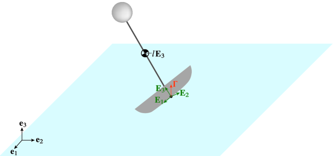
Figure 1. What we call the pendulum skate here is a simple model for a figure skater developed by Gzenda and Putkaradze [13]. The unit vector $\boldsymbol{\Gamma}$—the vertical upward direction seen from the body frame $\{\mathbf{E}_{i}\}_{i=1}^{3}$—is the advected parameter here.

Following [13] (see also Section 2.1 below), the configuration space is the semidirect product Lie group $\mathsf{SE}(3)\mathrel{\mathop{:}}=\mathsf{SO}(3)\ltimes\mathbb{R}^{3}$, or the matrix group

$$\mathsf{SE}(3)={\left\{(R,\mathbf{x})\mathrel{\mathop{:}}=\begin{bmatrix}R&\mathbf{x}\\ \mathbf{0}^{T}&1\end{bmatrix}\ |\ R\in\mathsf{SO}(3),\,\mathbf{x}\in\mathbb{R}^{3}\right\}}.$$ (1)

The gravity breaks the $\mathsf{SE}(3)$-symmetry of the pendulum skate, just as in the well-known example of the heavy top in the semidirect product theory of mechanics [17, 18, 15, 8]. Hence Gzenda and Putkaradze [13] used the unit vector $\boldsymbol{\Gamma}$—the vertical upward direction seen from the body frame as depicted in Figure 1 as in the heavy top equations—as an advected parameter vector, and derived its equations of motion as nonholonomic Euler–Poincaré equations with advected parameters on $\mathfrak{se}(3)\times(\mathbb{R}^{3})^{*}$, where $\mathfrak{se}(3)$ is the Lie algebra of $\mathsf{SE}(3)$ and the dual space $(\mathbb{R}^{3})^{*}$ of $\mathbb{R}^{3}$ is for advected parameters $\boldsymbol{\Gamma}$ that take care of the broken $\mathsf{SE}(3)$-symmetry.

It turns out that it is not just the gravity that breaks the symmetry. The constraints imposed by the rink—including the nonholonomic constraint that the skate cannot slide sideways—also break the symmetry as well. We shall treat this in detail later, but here is an intuitive explanation of why it breaks the symmetry: When we start off with the configuration space $\mathsf{SE}(3)$ without the gravity nor the rink, we have an ambient space without any preferred direction or orientation—hence the $\mathsf{SE}(3)$-symmetry. However, by introducing the rink to the setting, we effectively introduce a special direction—the unit normal vector to the rink—to the ambient space, thereby breaking the $\mathsf{SE}(3)$-symmetry. This is just like how the gravity breaks the symmetry by introducing the special “vertical” direction to the ambient space that would be otherwise uniform in any direction.

The main motivation for this work is to stabilize nonholonomic mechanical systems on Lie groups with such broken symmetry. We shall show in Section 5 that, for the pendulum skate, the upright spinning and upright sliding motions—ubiquitous in figure skating—are equilibria of the nonholonomic Euler–Poincaré equations derived in [13]. As the intuition suggests, the spinning equilibrium is stable only under certain conditions, whereas the sliding equilibrium is always unstable.

Motivated by the problem of finding a control law to stabilize the sliding equilibrium, we would like to extend the method of Controlled Lagrangians of Bloch et al. [3] to the Euler–Poincaré equations with symmetry-breaking nonholonomic constraints. Particularly, our main goal is to build on the nonholonomic Euler–Poincaré theory of Schneider [20] (see also Holm [14, Section 12.3]) to derive matching conditions for the Controlled Lagrangians applied to such systems.

The pendulum skate indeed necessitates a slight generalization of [20] because it does not fit into the most general setting of [20, Section 2.1 and Theorem 1]. We note that Gay-Balmaz and Yoshimura [12] made such a generalization in a more abstract and general Dirac structure setting. Our focus is rather on first having a concrete expression for the nonholonomic Euler–Poincaré equations, particularly on a systematic way to eliminate the Lagrange multipliers in the equations of motion arising from the constraints.

Developing a general method of controlled Lagrangians for nonholonomic systems is challenging, particularly because of the Lagrange multipliers. Indeed, extensions of the method of Controlled Lagrangians to nonholonomic systems are limited to a very special class of Lagrange–d’Alembert equations; see, e.g., Zenkov et al. [24, 25, 26, 28]. To our knowledge, an extension to nonholonomic Euler–Poincaré equations has been done by Schneider [20] only for the so-called Chaplygin top.

1.2. Main Results and Outline

We build on the work of Schneider [20] to develop matching conditions for mechanical systems on Lie group $\mathsf{S}$ with symmetry-breaking nonholonomic constraints. Particularly, we assume: (i) The left $\mathsf{S}$-invariance of the Lagrangian is broken, but can be recovered using an advected parameter $\Gamma$; (ii) the nonholonomic constraints are not left-invariant either, but this broken symmetry is also recovered by using the same $\Gamma$. We shall explain the details of this setting in Section 2 using the pendulum skate as an example.

In Section 3, we formulate the reduced Lagrange–d’Alembert principle and derive the nonholonomic Euler–Poincaré equations with broken symmetry as Proposition 5, giving a generalization of the General Theorem of Schneider [20, Theorem 1]. However, as mentioned earlier, it is a special case of the Dirac reduction for nonholonomic systems by Gay-Balmaz and Yoshimura [12], and is included here only for completeness.

The ideas that nonholonomic constraints may be symmetry-breaking and that the broken symmetry may be recovered using an advected parameter are not new; they were discussed in [20] as well as Tai [21], Burkhardt and Burdick [6], and Burkhardt [7]. Our treatment is more systematic as in [12] and applies to more general constraints than those of [20].

The above result leads to the notion of $\Gamma$-dependent quasivelocities in Section 4. Quasivelocities have been often used in nonholonomic mechanics; see, e.g., Bloch et al. [4], Ball et al. [2], Zenkov [23], Zenkov et al. [27] and references therein. However, to our knowledge, the idea of advected-parameter-dependent quasivelocities is new. Those $\Gamma$-dependent quasivelocities help us eliminate the Lagrange multipliers in the nonholonomic Euler–Poincaré equations derived in Proposition 5.

In Section 5, we apply the result from Section 4 to the pendulum skate, find a family of equilibria including the upright spinning and upright sliding ones, and analyze their stability.

In Section 6, we show that the nonholonomic Euler–Poincaré equations written in the $\Gamma$-dependent quasivelocities help us extend the Controlled Lagrangians of Bloch et al. [3]—developed for the standard Euler–Poincaré equation—to our nonholonomic setting. Indeed, the derivation and expressions of the resulting matching conditions in Proposition 13 are almost the same as those in [3] thanks to the formulation using the quasivelocities. The result also generalizes the simpler and ad-hoc matching of [20] for the Chaplygin top and our own for the pendulum skate in [11].

Finally, in Section 7, we apply the Controlled Lagrangian to find a feedback control to stabilize the sliding equilibrium, and illustrate the result in a numerical simulation.

2. Broken Symmetry in Lagrangian and Nonholonomic Constraints

In this section, we would like to use the pendulum skate of Gzenda and Putkaradze [13] to describe the basic ideas behind mechanical systems on Lie groups with symmetry-breaking nonholonomic constraints.

2.1. Pendulum Skate

Let $\{\mathbf{e}_{1},\mathbf{e}_{2},\mathbf{e}_{3}\}$ and $\{\mathbf{E}_{1},\mathbf{E}_{2},\mathbf{E}_{3}\}$ be the spatial and body frames, respectively, where the body frame is aligned with the principal axes of inertia; particularly $\mathbf{E}_{1}$ is aligned with the edge of the blade as shown in Figure 1. The two frames are related by the rotation matrix $R(t)\in\mathsf{SO}(3)$ whose column vectors represent the body frame viewed in the spatial one at time $t$.

The origin of the body frame is the blade-ice contact point, and has position vector $\mathbf{x}(t)=(x_{1}(t),x_{2}(t),0)$ at time $t$ in the spatial frame. However, we shall treat the position $\mathbf{x}$ of the contact point as a vector in $\mathbb{R}^{3}$ and impose $x_{3}=0$ as a constraint. Hence, as mentioned earlier, the configuration space is the semidirect product Lie group $\mathsf{SE}(3)\mathrel{\mathop{:}}=\mathsf{SO}(3)\ltimes\mathbb{R}^{3}$ from (1), where the multiplication rule is given by

$$(R_{0},\mathbf{x}_{0})\cdot(R,\mathbf{x})=(R_{0}R,R_{0}\mathbf{x}+\mathbf{x}_{0}).$$

Let us find the Lagrangian of the system. If $t\mapsto s(t)=(R(t),\mathbf{x}(t))$ is the dynamics of the system in $\mathsf{SE}(3)$, then

$$s^{-1}\dot{s}=\begin{bmatrix}R^{T}\dot{R}&R^{T}\dot{\mathbf{x}}\\ \mathbf{0}^{T}&0\end{bmatrix}=\mathrel{\mathop{:}}\begin{bmatrix}\hat{\Omega}&\mathbf{Y}\\ \mathbf{0}^{T}&0\end{bmatrix}=\mathrel{\mathop{:}}(\hat{\Omega},\mathbf{Y})\in\mathfrak{se}(3),$$

where $\hat{\Omega}\mathrel{\mathop{:}}=R^{T}\dot{R}$ is the body angular velocity; $\mathbf{Y}\mathrel{\mathop{:}}=R^{T}\dot{\mathbf{x}}$ is the velocity of the blade-ice contact point seen from the body frame.

Suppose that the center of mass is located at ${l\mathbf{E}_{3}}$ in the body frame as shown in Figure 1, and hence, in the spatial frame, is located at $\mathbf{x}_{\text{cm}}(t)\mathrel{\mathop{:}}=\mathbf{x}(t)+lR(t)\mathbf{E}_{3}$. Then, the Lagrangian $L_{\mathbf{e}_{3}}\colon T\mathsf{SE}(3)\to\mathbb{R}$ is given by:

$$L_{\mathbf{e}_{3}}{\left(R,\mathbf{x},\dot{R},\dot{\mathbf{x}}\right)} \mathrel{\mathop{:}}=\frac{1}{2}\mathop{\mathrm{tr}}\nolimits{\left(\dot{R}\mathbb{J}\dot{R}^{T}\right)}+\frac{m}{2}{\left\|\dot{\mathbf{x}}_{\text{cm}}\right\|}^{2}-m\mathrm{g}\mathbf{e}_{3}^{T}\mathbf{x}_{\text{cm}}$$

$$=\frac{1}{2}\mathop{\mathrm{tr}}\nolimits{\left(R^{T}\dot{R}\mathbb{J}\dot{R}^{T}R\right)}+\frac{m}{2}{\left\|\dot{\mathbf{x}}+\dot{R}l\mathbf{E}_{3}\right\|}^{2}-m\mathrm{g}l\mathbf{e}_{3}^{T}R\mathbf{E}_{3}$$

$$=\frac{1}{2}\mathop{\mathrm{tr}}\nolimits{\left(\hat{\Omega}\mathbb{J}\hat{\Omega}^{T}\right)}+\frac{m}{2}{\left\|\mathbf{Y}+l\hat{\Omega}\mathbf{E}_{3}\right\|}^{2}-m\mathrm{g}l(R^{T}\mathbf{e}_{3})^{T}\mathbf{E}_{3},$$

where $m$ is the total mass, $\mathrm{g}$ is the gravitational acceleration, $\|\cdot\|$ is the Euclidean norm, and $\mathbb{J}$ is the inertia matrix.

We also identify ${\boldsymbol{\Omega}=(\Omega_{1},\Omega_{2},\Omega_{3})\in\mathbb{R}^{3}}$ with $\hat{\Omega}\in\mathfrak{so}(3)$ via the hat map [16, §5.3]:

$$\widehat{(\,\cdot\,)}\colon{\mathbb{R}}^{3}\to\mathfrak{se}(3);\qquad\boldsymbol{\Omega}\mapsto\hat{\Omega}=\begin{bmatrix}0&\mkern-15.0mu-\Omega_{3}&\Omega_{2}\\ \mkern 8.0mu\Omega_{3}&\mkern-6.0mu0&\mkern-8.0mu-\Omega_{1}\\ -\Omega_{2}&\Omega_{1}&0\end{bmatrix}.$$

Then we have the following correspondence with the cross product: $\hat{\Omega}\mathbf{y}=\boldsymbol{\Omega}\times\mathbf{y}$ for every $\mathbf{y}\in\mathbb{R}^{3}$. So we may use ${(\boldsymbol{\Omega},\mathbf{Y})\in\mathbb{R}^{3}\times\mathbb{R}^{3}}$ as coordinates for $\mathfrak{se}(3)\cong\mathbb{R}^{3}\times\mathbb{R}^{3}$, and we have

$$L_{\mathbf{e}_{3}}{\left(R,\mathbf{x},\dot{R},\dot{\mathbf{x}}\right)}=\frac{1}{2}\boldsymbol{\Omega}^{T}\mathbb{I}\boldsymbol{\Omega}+\frac{m}{2}{\left\|\mathbf{Y}+l\boldsymbol{\Omega}\times\mathbf{E}_{3}\right\|}^{2}-m\mathrm{g}l(R^{T}\mathbf{e}_{3})^{T}\mathbf{E}_{3},$$

where $\mathbb{I}\mathrel{\mathop{:}}=\mathop{\mathrm{tr}}\nolimits(\mathbb{J})\mathsf{I}-\mathbb{J}=\operatorname{diag}(I_{1},I_{2},I_{3})$ with $\mathsf{I}$ being the $3\times 3$ identity matrix is the (body) moment of inertia tensor; see, e.g., Holm et al. [16, ​§7.1].

The Lagrangian does not possess the full $\mathsf{SE}(3)$-symmetry due to the gravity. Indeed, if $R_{0}^{T}\mathbf{e}_{3}\neq\mathbf{e}_{3}$ then, in general,

$$L_{\mathbf{e}_{3}}{\left(R_{0}R,R_{0}\mathbf{x}+\mathbf{x}_{0},R_{0}\dot{R},R_{0}\dot{\mathbf{x}}\right)}\neq L_{\mathbf{e}_{3}}{\left(R,\mathbf{x},\dot{R},\dot{\mathbf{x}}\right)},$$ (2)

although the equality holds if $R_{0}^{T}\mathbf{e}_{3}=\mathbf{e}_{3}$. In the next subsection, we shall discuss a general theory on how to recover the full symmetry of such a Lagrangian with broken symmetry, and come back to the pendulum skate as an example.

2.2. Broken Symmetry in Lagrangian

Let $L_{\gamma_{0}}\colon T\mathsf{S}\to\mathbb{R}$ be a Lagrangian with a fixed parameter $\gamma_{0}\in X^{*}$, where $X^{*}$ is the dual of a vector space $X$. For each $s_{0}\in\mathsf{S}$, let $\mathsf{L}_{s_{0}}\colon\mathsf{S}\to\mathsf{S};s\mapsto s_{0}s$ be the left translation, and $T\mathsf{L}_{s_{0}}\colon\dot{s}\mapsto T\mathsf{L}_{s_{0}}(\dot{s})=\mathrel{\mathop{:}}s_{0}\dot{s}$ be its tangent lift. Suppose that the Lagrangian is not $\mathsf{S}$-invariant, i.e., $L_{\gamma_{0}}\circ T\mathsf{L}_{s_{0}}\neq L_{\gamma_{0}}$ for some $s_{0}\in\mathsf{S}$. We also assume that we can recover the broken symmetry as follows: Define the extended Lagrangian $L\colon T\mathsf{S}\times X^{*}\to\mathbb{R}$ so that

$$L(s,\dot{s},\gamma_{0})=L_{\gamma_{0}}(s,\dot{s})\quad\forall(s,\dot{s})\in T\mathsf{S},$$

and suppose that there is a representation

$$\mathsf{S}\times X\to X;\qquad(s,\mathsf{x})\mapsto s\mathsf{x}.$$ (3)

as well as its induced representation $(s,\gamma)\mapsto s\gamma$ on $X^{*}$, i.e.,

$$\mathsf{S}\times X^{*}\to X^{*};\qquad(s,\gamma)\mapsto s\gamma\quad\text{such that}\quad{\left\langle s\gamma,\mathsf{x}\right\rangle}={\left\langle\gamma,s^{-1}\mathsf{x}\right\rangle}\quad\forall\mathsf{x}\in X.$$ (4)

We assume that we can recover the (left) $\mathsf{S}$-symmetry as follows: For every $s_{0},s\in\mathsf{S}$ and every $\gamma\in X^{*}$,

$$L(s_{0}s,s_{0}\dot{s},s_{0}\gamma)=L(s,\dot{s},\gamma).$$

As a result, we may define the reduced Lagrangian as follows:

$$\ell\colon\mathfrak{s}\times X^{*}\to\mathbb{R};\qquad\ell(\xi,\Gamma)\mathrel{\mathop{:}}=L(e,\xi,\Gamma),$$ (5)

where $\mathfrak{s}$ is the Lie algebra of $\mathsf{S}$.

Example 1 (Lagrangian of pendulum skate [13]).

For the pendulum skate from Section 2.1, we define the extended Lagrangian $L\colon T^{*}\mathsf{SE}(3)\times(\mathbb{R}^{3})^{*}\to\mathbb{R}$ as follows:

$$L{\left(R,\mathbf{x},\dot{R},\dot{\mathbf{x}},\boldsymbol{\gamma}\right)}=\frac{1}{2}\boldsymbol{\Omega}^{T}\mathbb{I}\boldsymbol{\Omega}+\frac{m}{2}{\left\|\mathbf{Y}+l\boldsymbol{\Omega}\times\mathbf{E}_{3}\right\|}^{2}-m\mathrm{g}l(R^{T}\boldsymbol{\gamma})^{T}\mathbf{E}_{3}$$

so that $L{\left(R,\mathbf{x},\dot{R},\dot{\mathbf{x}},\mathbf{e}_{3}\right)}=L_{\mathbf{e}_{3}}{\left(R,\mathbf{x},\dot{R},\dot{\mathbf{x}}\right)}$.

We also define an $\mathsf{SE}(3)$-representation on $\mathbb{R}^{3}$ by setting $(R,\mathbf{x})\mathbf{y}\mathrel{\mathop{:}}=R\mathbf{y}$. Then, identifying $(\mathbb{R}^{3})^{*}$ with $\mathbb{R}^{3}$ via the dot product, we have

$${\left((R,\mathbf{x})\boldsymbol{\gamma}\right)}\cdot\mathbf{y}=\boldsymbol{\gamma}\cdot{\left((R,\mathbf{x})^{-1}\mathbf{y}\right)}=\boldsymbol{\gamma}\cdot{\left(R^{-1}\mathbf{y}\right)}=(R\boldsymbol{\gamma})\cdot\mathbf{y}.$$

Therefore, we have

$$\mathsf{SE}(3)\times(\mathbb{R}^{3})^{*}\to(\mathbb{R}^{3})^{*};\qquad((R,\mathbf{x}),\boldsymbol{\gamma})\mapsto R\boldsymbol{\gamma}$$ (6)

using the standard matrix-vector multiplication.

Then we see that the $\mathsf{SE}(3)$-symmetry is recovered: For every $(R_{0},\mathbf{x}_{0}),(R,\mathbf{x})\in\mathsf{SE}(3)$ and every $\boldsymbol{\gamma}\in\mathbb{R}^{3}$,

$$L{\left(R_{0}R,R_{0}\mathbf{x}+\mathbf{x}_{0},R_{0}\dot{R},R_{0}\dot{\mathbf{x}},R_{0}\boldsymbol{\gamma}\right)}=L{\left(R,\mathbf{x},\dot{R},\dot{\mathbf{x}},\boldsymbol{\gamma}\right)}.$$

Therefore, we may define the reduced Lagrangian

$$\begin{split}&\ell\colon\mathfrak{se}(3)\times(\mathbb{R}^{3})^{*}\cong\mathbb{R}^{3}\times\mathbb{R}^{3}\times\mathbb{R}^{3}\to\mathbb{R};\\ &\ell(\boldsymbol{\Omega},\mathbf{Y},\boldsymbol{\Gamma})\mathrel{\mathop{:}}=\frac{1}{2}\boldsymbol{\Omega}^{T}\mathbb{I}\boldsymbol{\Omega}+\frac{m}{2}{\left\|\mathbf{Y}+l\boldsymbol{\Omega}\times\mathbf{E}_{3}\right\|}^{2}-m\mathrm{g}l\boldsymbol{\Gamma}^{T}\mathbf{E}_{3},\end{split}$$ (7)

which agrees with [13, Eq. (1)]. Since $\gamma_{0}=\mathbf{e}_{3}$ for our Lagrangian, the advected parameter is $\boldsymbol{\Gamma}=R^{T}\gamma_{0}=R^{T}\mathbf{e}_{3}$, which gives the vertical upward direction (essentially the direction of gravity) seen from the body frame; see Figure 1.

Remark 2 (Intuition behind symmetry recovery).

Here is an intuitive interpretation of how the symmetry recovery works in Example 1 above. When we talked about the broken $\mathsf{SE}(3)$-symmetry in (2), the vertical upward direction $\mathbf{e}_{3}$ (essentially the direction of gravity) was fixed, and the $\mathsf{SE}(3)$-action $(R_{0},\mathbf{x}_{0})\cdot(R,\mathbf{x})=(R_{0}R,R_{0}\mathbf{x}+\mathbf{x}_{0})$ rotates the pendulum skate by $R_{0}$ and translates it by $\mathbf{x}_{0}$ but left the direction of the gravity unchanged, resulting in a system whose direction of gravity is different from the original configuration $(R,\mathbf{x})$; hence the symmetry is broken. On the other hand, when we introduced $\boldsymbol{\gamma}$ as a new variable in the Lagrangian above and let $\mathsf{SE}(3)$ act on $\gamma$ as defined in (6), we co-rotated the direction of the gravity along with the pendulum skate, resulting in a system with the same relative direction of gravity as the original one; hence the whole system—now involving the variable direction of gravity—possesses the $\mathsf{SE}(3)$-symmetry.

2.3. Broken Symmetry in Nonholonomic Constraints

Following Gay-Balmaz and Yoshimura [12, Section 4.2], we assume that the system is subject to nonholonomic constraints with a fixed parameter $\gamma_{0}\in X^{*}$, that is, the constraint is defined by a corank $r$ smooth distribution $\mathcal{D}_{\gamma_{0}}\subset T\mathsf{S}$ so that the dynamics $t\mapsto s(t)\in\mathsf{S}$ satisfies $\dot{s}(t)\in\mathcal{D}_{\gamma_{0}}(s(t))$. In other words, we have one-forms $\{\Psi^{a}_{\gamma_{0}}\}_{a=1}^{r}$ on $\mathsf{S}$ such that the annihilator $\mathcal{D}_{\gamma_{0}}^{\circ}(s)=\mathop{\mathrm{span}}\nolimits\{\Psi^{a}_{\gamma_{0}}(s)\}_{a=1}^{r}$, i.e., $\dot{s}(t)\in\ker\Psi^{a}_{\gamma_{0}}(s(t))$ for any $a\in\{1,\dots,r\}$.

We assume that $\mathcal{D}_{\gamma_{0}}$ is not $\mathsf{S}$-invariant, i.e.,

$$T_{s}\mathsf{L}_{s_{0}}(\mathcal{D}_{\gamma_{0}}(s))\neq\mathcal{D}_{\gamma_{0}}(s_{0}s)\ \text{for some}\ s,s_{0}\in\mathsf{S},$$

or in terms of the one-forms,

$$(\mathsf{L}_{s_{0}}^{*}\Psi^{a}_{\gamma_{0}})(s)\neq\Psi^{a}_{\gamma_{0}}(s)\ \text{for some}\ s,s_{0}\in\mathsf{S}\ \text{and some}\ a\in\{1,\dots,r\}.$$

We also assume that we may recover the $\mathsf{S}$-symmetry in a similar way as above: Defining

$$\mathcal{D}\colon\mathsf{S}\times X^{*}\to T\mathsf{S}\quad\text{with}\quad\mathcal{D}(s,\gamma)\subset T_{s}\mathsf{S}\quad\text{and}\quad\mathcal{D}(s,\gamma_{0})=\mathcal{D}_{\gamma_{0}}(s)\quad\forall s\in\mathsf{S},$$

we have the $\mathsf{S}$-invariance in the following sense:

$$T_{s}\mathsf{L}_{s_{0}}(\mathcal{D}(s,\gamma))=\mathcal{D}(s_{0}s,s_{0}\gamma)\quad\forall s,s_{0}\in\mathsf{S}\quad\forall\gamma\in X^{*}.$$

In other words, we have the following $r$ one-forms on $\mathsf{S}$ with a parameter in $X^{*}$:

$$\Psi^{a}\colon\mathsf{S}\times X^{*}\to T^{*}\mathsf{S}\quad\text{with}\quad\Psi^{a}(s,\gamma)\subset T_{s}^{*}\mathsf{S}\quad\forall s\in\mathsf{S}\quad\forall\gamma\in X^{*}\quad\forall a\in\{1,\dots,r\}$$

satisfying $\mathcal{D}^{\circ}(s,\gamma)=\mathop{\mathrm{span}}\nolimits\{\Psi^{a}(s,\gamma)\}_{a=1}^{r}$ and

$$(\mathsf{L}_{s_{0}}^{*}\Psi^{a})(\,\cdot\,,s_{0}\gamma)=\Psi^{a}(\,\cdot\,,\gamma)\quad\forall\gamma\in X^{*}\quad\forall a\in\{1,\dots,r\}.$$ (8)

We may then define the following parameter-dependent subspaces in $\mathfrak{s}$ and parameter-dependent elements in $\mathfrak{s}^{*}$:

$$\mathfrak{d}(\Gamma)\mathrel{\mathop{:}}=\mathcal{D}(e,\Gamma)\subset\mathfrak{s},\qquad\psi^{a}(\Gamma)\mathrel{\mathop{:}}=\Psi^{a}(e,\Gamma)\in\mathfrak{s}^{*}\quad\forall a\in\{1,\dots,r\}$$ (9)

so that the annihilator $\mathfrak{d}^{\circ}(\Gamma)=\mathop{\mathrm{span}}\nolimits\{\psi^{a}(\Gamma)\}_{a=1}^{r}\subset\mathfrak{s}^{*}$.

Example 3 (No-side-sliding constraint of pendulum skate).

The skate blade moves without friction, but with a constraint that prohibits motions perpendicular to its edge. This means that the spatial velocity $\dot{\mathbf{x}}$ has no components in the direction perpendicular to the plane spanned by $\{R\mathbf{E}_{1},\mathbf{e}_{3}\}$, i.e., ${\left\langle\dot{\mathbf{x}},R\mathbf{E}_{1}\times\mathbf{e}_{3}\right\rangle}=0$ as shown in Figure 2. In other words, setting $\Psi_{\mathbf{e}_{3}}(R,\mathbf{x})=(R\mathbf{E}_{1}\times\mathbf{e}_{3})^{T}{\bf d}\mathbf{x}$, one may write the constraint as $\dot{\mathbf{x}}\in\ker\Psi_{\mathbf{e}_{3}}$.

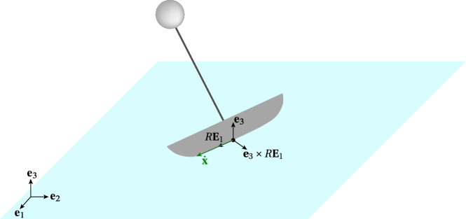
Figure 2. No side sliding.

It is easy to see that the $\mathsf{SE}(3)$-symmetry is broken: If we take $(R_{0},\mathbf{x}_{0})\in\mathsf{SE}(3)$ with $R_{0}^{T}\mathbf{e}_{3}\neq\mathbf{e}_{3}$, then

$$(\mathsf{L}_{(R_{0},\mathbf{x}_{0})}^{*}\Psi_{\mathbf{e}_{3}})(R,\mathbf{x}) =((R_{0}R\mathbf{E}_{1})\times\mathbf{e}_{3})^{T}{\bf d}(R_{0}\mathbf{x})$$

$$={\left((R\mathbf{E}_{1})\times(R_{0}^{T}\mathbf{e}_{3})\right)}^{T}{\bf d}\mathbf{x}$$

$$\neq\Psi_{\mathbf{e}_{3}}(R,\mathbf{x})$$

in general, although $\mathsf{L}_{(R_{0},\mathbf{x}_{0})}^{*}\Psi_{\mathbf{e}_{3}}=\Psi_{\mathbf{e}_{3}}$ if $R_{0}^{T}\mathbf{e}_{3}=\mathbf{e}_{3}$.

One notices that this is the same type of broken symmetry as in the Lagrangian from Example 1 caused by the gravity. This suggests the same remedy applied to the Lagrangian would recover the $\mathsf{SE}(3)$-symmetry of the constraint too. Indeed, define

$$\Psi\colon\mathsf{SE}(3)\times(\mathbb{R}^{3})^{*}\to T^{*}\mathsf{SE}(3);\qquad\Psi((R,\mathbf{x}),\boldsymbol{\gamma})\mathrel{\mathop{:}}=((R\mathbf{E}_{1})\times\boldsymbol{\gamma})^{T}{\bf d}\mathbf{x}$$

so that $\Psi((R,\mathbf{x}),\mathbf{e}_{3})=\Psi_{\mathbf{e}_{3}}(R,\mathbf{x})$. Then we see that, for every $(R_{0},\mathbf{x}_{0}),(R,\mathbf{x})\in\mathsf{SE}(3)$ and every $\boldsymbol{\gamma}\in\mathbb{R}^{3}$,

$$(\mathsf{L}_{(R_{0},\mathbf{x}_{0})}^{*}\Psi)((R,\mathbf{x}),R_{0}\boldsymbol{\gamma}) ={\left((R_{0}R\mathbf{E}_{1})\times(R_{0}\boldsymbol{\gamma})\right)}^{T}{\bf d}(R_{0}\mathbf{x})$$

$$={\left((R\mathbf{E}_{1})\times\boldsymbol{\gamma}\right)}^{T}{\bf d}\mathbf{x}$$

$$=\Psi((R,\mathbf{x}),\boldsymbol{\gamma}).$$

Therefore, we define the $\boldsymbol{\Gamma}$-dependent element

$$\psi^{3}(\boldsymbol{\Gamma})\mathrel{\mathop{:}}=\Psi((I,\mathbf{0}),\boldsymbol{\Gamma})=(\mathbf{0},\mathbf{E}_{1}\times\boldsymbol{\Gamma})\in\mathfrak{se}(3)^{*}\cong\mathbb{R}^{3}\times\mathbb{R}^{3},$$

where we used the superscript $3$ because there are two other constraints as we shall see in Example 8.

Remark 4.

Why does the same advected parameter $\boldsymbol{\Gamma}$—which we used to recover the broken symmetry due to the gravity—work in order to recover the broken symmetry due to the nonholonomic constraint as well? The nonholonomic constraint is characterized by how one introduces the rink into the system. In this problem, we introduced the rink as a horizontal plane—perpendicular to the direction of gravity. So $\boldsymbol{\Gamma}$ gives both the direction of gravity and the orientation of the rink seen from the body frame.

3. Nonholonomic Euler–Poincaré Equation with Advected Parameters

This section gives a review of the reduced Lagrange–d’Alembert principle for mechanical systems with broken symmetry. Our result gives a slight generalization of the General Theorem of Schneider [20, Theorem 1]. However, as mentioned earlier, ours is a special case of Gay-Balmaz and Yoshimura [12, Theorem 4.3] as well, and so we include this result only for completeness.

3.1. Reduced Lagrange–d’Alembert Principle with Broken Symmetry

We would like to find the reduced equations of motion exploiting the recovered symmetry. For our setting, one needs to turn the variational principle of Holm et al. [15, Theorem 3.1] (see also Cendra et al. [8, Theorem 1.1]) into a Lagrange–d’Alembert-type incorporating the symmetry-breaking nonholonomic constraints. We note that this is done in Schneider [20, Theorem 1] with a semidirect product Lie group $\mathsf{S}=\mathsf{G}\ltimes V$ assuming a special class of nonholonomic constraints.

Before describing our version of the reduced Lagrange–d’Alembert principle with broken symmetry, let us introduce some notation used in the result to follow. For any curve $t\mapsto s(t)\in\mathsf{S}$, we define $t\mapsto\xi(t)\mathrel{\mathop{:}}=s(t)^{-1}\dot{s}(t)\in\mathfrak{s}$; conversely, given $t\mapsto\xi(t)\in\mathfrak{s}$, we define $t\mapsto s(t)\in\mathsf{S}$ via $\dot{s}(t)=s(t)\xi(t)$ with the left translation. Similarly, for any (infinitesimal) variation $t\mapsto\delta s(t)\in T_{s(t)}\mathsf{S}$ of the curve $t\mapsto s(t)$, we define $t\mapsto\eta(t)\mathrel{\mathop{:}}=s(t)^{-1}\delta s(t)$ and conversely as well.

We shall also use the Lie algebra representation

$$\mathfrak{s}\times X\to X;\qquad(\xi,\mathsf{x})\mapsto\left.\frac{d}{d\varepsilon}\exp(\varepsilon\xi)\mathsf{x}\right|_{\varepsilon=0}=\mathrel{\mathop{:}}\xi\mathsf{x},$$

and

$$\mathfrak{s}\times X^{*}\to X^{*};\qquad(\xi,\gamma)\mapsto\xi\gamma\quad\text{so that}\quad{\left\langle\xi\gamma,\mathsf{x}\right\rangle}=-{\left\langle\gamma,\xi\mathsf{x}\right\rangle}\quad\forall\mathsf{x}\in X,$$ (10)

as well as the momentum map $\mathbf{K}\colon X\times X^{*}\to\mathfrak{s}^{*}$ defined by

$${\left\langle\mathbf{K}(\mathsf{x},\Gamma),\xi\right\rangle}={\left\langle\Gamma,\xi\mathsf{x}\right\rangle}=-{\left\langle\xi\Gamma,\mathsf{x}\right\rangle}\quad\forall\xi\in\mathfrak{s},$$ (11)

where $\xi\mathsf{x}$ is defined in the similar way as in (10) using (3).

Also, for any smooth function $f\colon E\to\mathbb{R}$ on a real vector space $E$, let us define its functional derivative $\delta f/\delta x\in E^{*}$ at $x\in E$ such that, for any $\delta x\in E$, under the natural dual pairing ${\left\langle\,\cdot\,,\,\cdot\,\right\rangle}\colon E^{*}\times E\to\mathbb{R}$,

$${\left\langle\frac{\delta f}{\delta x},\delta x\right\rangle}=\left.\frac{d}{d\varepsilon}f(x+\varepsilon\delta x)\right|_{\varepsilon=0}.$$

Proposition 5 (Reduced Lagrange–d’Alembert Principle with Broken Symmetry).

Let $\gamma_{0}\in X^{*}$ be fixed, and suppose that the Lagrangian $L_{\gamma_{0}}\colon T\mathsf{S}\to\mathbb{R}$ and the distribution $\mathcal{D}_{\gamma_{0}}\subset T\mathsf{S}$ defining nonholonomic constraints satisfy the assumptions on symmetry recovery from Sections 2.2 and 2.3.

Then the following are equivalent:

1. The curve $t\mapsto s(t)\in\mathsf{S}$ with the constraint $\dot{s}(t)\in\mathcal{D}_{\gamma_{0}}(s(t))$ satisfies the Lagrange–d’Alembert principle

   $$\delta\int_{t_{0}}^{t_{1}}L_{\gamma_{0}}{\left(s(t),\dot{s}(t)\right)}\,dt=0$$

   subject to $\delta s(t_{0})=\delta s(t_{1})=0$ and $\delta s(t)\in\mathcal{D}_{\gamma_{0}}(s(t))$ for any $t\in(t_{0},t_{1})$.

2. The curve $t\mapsto\xi(t)\in\mathfrak{s}$ along with

   $$t\mapsto\Gamma(t)\mathrel{\mathop{:}}=s(t)^{-1}\gamma_{0}\in X^{*}$$ (12)

   and with the constraint

   $$\xi(t)\in\mathfrak{d}(\Gamma(t))\iff{\left\langle\psi^{a}(\Gamma(t)),\xi(t)\right\rangle}=0\quad\forall t\in[t_{0},t_{1}]\quad\forall a\in\{1,\dots,r\}$$ (13)

   satisfies the following reduced Lagrange–d’Alembert principle in terms of the reduced Lagrangian $\ell\colon\mathfrak{s}\times X^{*}\to\mathbb{R}$ defined in (5):

   $$\delta\int_{t_{0}}^{t_{1}}\ell(\xi(t),\Gamma(t))\,dt=0,$$ (14)

   where variations of $t\mapsto(\xi(t),\Gamma(t))$ are subject to the constraints

   $$\delta\xi=\dot{\eta}+\operatorname{ad}_{\xi}\eta,\qquad\delta\Gamma=-\eta\,\Gamma$$ (15)

   for every curve $t\mapsto\eta(t)\in\mathfrak{s}$ satisfying

   $$\delta\eta(t_{0})=\delta\eta(t_{1})=0,\qquad{\left\langle\psi^{a}(\Gamma(t)),\eta(t)\right\rangle}=0\quad\forall t\in[t_{0},t_{1}]\quad\forall a\in\{1,\dots,r\}.$$ (16)

3. The curve $t\mapsto(\xi(t),\Gamma(t))$ with $\xi(t)\in\mathfrak{d}(\Gamma(t))$ satisfies the nonholonomic Euler–Poincaré equations with advected parameter $\Gamma$:

   $$\frac{d}{dt}{\left(\frac{\delta\ell}{\delta\xi}\right)} =\operatorname{ad}_{\xi}^{*}\frac{\delta\ell}{\delta\xi}+\mathbf{K}{\left(\frac{\delta\ell}{\delta\Gamma},\Gamma\right)}+\lambda_{a}\psi^{a}(\Gamma),$$ (17a)

   $$\dot{\Gamma} =-\xi\Gamma$$ (17b)

   with $\Gamma(t_{0})=s(t_{0})^{-1}\gamma_{0}$, where $\{\lambda_{a}\}_{a=1}^{r}$ are Lagrange multipliers.

Proof.

Let us first show the equivalence between (i) and (16). First, let us show that the two action integrals are equal. Indeed, using the definition (5) of $\ell$,

$$L_{\gamma_{0}}(s,\dot{s})=L(s,\dot{s},\gamma_{0})=L{\left(e,s^{-1}\dot{s},s^{-1}\gamma_{0}\right)}=\ell(\xi,\Gamma).$$

It is a standard result in the Euler–Poincaré theory that all variations of $t\mapsto s(t)$ with fixed endpoints induce and are induced by variations of $t\mapsto\xi(t)$ of the form $\delta\xi=\dot{\eta}+\operatorname{ad}_{\xi}\eta$ with $\eta$ vanishing at the endpoint; see, e.g., [15, Theorem 3.1 and Lemma 3.2]. Also, $\delta\Gamma=-\eta\Gamma$ easily follows from the definitions (10) and (12). Finally, one can show the equivalence between the nonholonomic constraints on $\delta s$ and $\eta$ as follows: For every $a\in\{1,\dots,r\}$,

$$\delta s\in\mathcal{D}_{\gamma_{0}}(s)\iff 0 ={\left\langle\Psi^{a}(s,\gamma_{0}),\delta s\right\rangle}$$

$$={\left\langle\Psi^{a}(s,\gamma_{0}),ss^{-1}\delta s\right\rangle}$$

$$={\left\langle(L_{s}^{*}\Psi^{a})(e,\gamma_{0}),\eta\right\rangle}$$

$$={\left\langle\Psi^{a}(e,s^{-1}\gamma_{0}),\eta\right\rangle}\quad(\because\eqref{eq:A-symmetry})$$

$$={\left\langle\psi^{a}(\Gamma),\eta\right\rangle}\quad(\because\text{\eqref{eq:a-def} and definition of $\Gamma$}).$$

It remains to show the equivalence between (16) and (17). As is done in the proof of [15, Theorem 3.1],

$$\delta\int_{t_{0}}^{t_{1}}\ell(\xi(t),\Gamma(t))\,dt =\int_{t_{0}}^{t_{1}}{\left({\left\langle\frac{\delta\ell}{\delta\xi},\delta\xi\right\rangle}+{\left\langle\delta\Gamma,\frac{\delta\ell}{\delta\Gamma}\right\rangle}\right)}dt$$

$$=\int_{t_{0}}^{t_{1}}{\left({\left\langle\frac{\delta\ell}{\delta\xi},\dot{\eta}+\operatorname{ad}_{\xi}\eta\right\rangle}-{\left\langle\eta\Gamma,\frac{\delta\ell}{\delta\Gamma}\right\rangle}\right)}dt$$

$$=-\int_{t_{0}}^{t_{1}}{\left\langle\frac{d}{dt}{\left(\frac{\delta\ell}{\delta\xi}\right)}-\operatorname{ad}_{\xi}^{*}\frac{\delta\ell}{\delta\xi}-\mathbf{K}{\left(\frac{\delta\ell}{\delta\Gamma},\Gamma\right)},\eta\right\rangle}dt.$$

Therefore, the reduced Lagrange–d’Alembert principle (14) with the nonholonomic constraints (16) yields (17a), whereas taking the time derivative of (12) yields (17b). Conversely, it is clear that (17a) implies (14) with the constraints imposed in (16), and integrating (17b) with the initial condition on $\Gamma$ given in (17) yields (12). ∎

Example 6 (General Theorem of Schneider [20, Theorem 1]).

Let $\mathsf{G}$ be a Lie group, $V$ be a vector space, and construct the semidirect product Lie group $\mathsf{S}\mathrel{\mathop{:}}=\mathsf{G}\ltimes V$ under the multiplication

$$s_{1}\cdot s_{2}=(g_{1},x_{1})\cdot(g_{2},x_{2})=(g_{1}g_{2},g_{1}x_{2}+x_{1}),$$

where $\mathsf{G}\times V\to V;(g,x)\mapsto gx$ is a representation. In what follows, we shall use the other induced $\mathsf{G}$- and $\mathfrak{g}$-representations on $V$ and $V^{*}$ defined in the same way we did for $X$ and $X^{*}$ above, as well as the associated momentum map $\mathbf{J}\colon V\times V^{*}\to\mathfrak{g}^{*}$ defined in the same way as $\mathbf{K}$ was in (11). Indeed, it is also assumed in [20] that $X=V$ and the $\mathsf{S}$-representation on $X^{*}$ is defined as $(g,x)\gamma\mathrel{\mathop{:}}=g\gamma$ using the $\mathsf{G}$-representation on $V^{*}$ induced by the above $\mathsf{G}$-representation on $V$. Hence, writing $\xi=(\Omega,Y)\in\mathfrak{s}=\mathfrak{g}\ltimes V$, it follows that $\xi\gamma=(\Omega,Y)\gamma=\Omega\gamma$ as well. It is then straightforward to see that, for every $(\Omega_{i},Y_{i})\in\mathfrak{s}=\mathfrak{g}\ltimes V$ with $i=1,2$,

$$\operatorname{ad}_{(\Omega_{1},Y_{1})}(\Omega_{2},Y_{2})\mathrel{\mathop{:}}=[(\Omega_{1},Y_{1}),(\Omega_{2},Y_{2})]={\left(\operatorname{ad}_{\Omega_{1}}\!\Omega_{2},\,\Omega_{1}Y_{2}-\Omega_{2}Y_{1}\right)},$$

What correspond to $\xi,\eta\in\mathfrak{s}=\mathfrak{g}\ltimes V$ in this example are

$$(\Omega,Y) \mathrel{\mathop{:}}=(g,x)^{-1}(\dot{g},\dot{x})={\left(g^{-1}\dot{g},g^{-1}\dot{x}\right)},$$

$$(\Sigma,Z) \mathrel{\mathop{:}}=(g,x)^{-1}(\delta{g},\delta{x})={\left(g^{-1}\delta{g},g^{-1}\delta{x}\right)},$$

respectively. Then the constraint on $\xi$ in (15) becomes

$$(\delta\Omega,\delta Y)=(\dot{\Omega},\dot{Y})+{\left(\operatorname{ad}_{\Omega}\!\Sigma,\,\Omega Z-\Sigma Y\right)},$$ (18)

In [20], the nonholonomic constraints are assumed to be in the form

$${\left\langle\Psi((g,x),\gamma),(\dot{g},\dot{x})\right\rangle}=\dot{x}-\bar{\Psi}((g,x),\gamma)\dot{g}=0\quad\text{with}\quad\bar{\Psi}((g,x),\gamma)\colon T_{g}\mathsf{G}\to V$$

with the following (left) $\mathsf{S}$-invariance:

$$\Psi((g_{0},x_{0})\cdot(g,x),(g_{0},x_{0})\gamma)=\Psi((g,x),\gamma)\quad\forall(g_{0},x_{0}),(g,x)\in\mathsf{S}\quad\forall\gamma\in X^{*}.$$

Hence we have

$${\left\langle\psi(\Gamma),(\Omega,Y)\right\rangle}\mathrel{\mathop{:}}=Y-\bar{\psi}(\Gamma)\Omega\quad\text{with}\quad\bar{\psi}(\Gamma)\mathrel{\mathop{:}}=\bar{\Psi}(e,\Gamma),$$

and thus the nonholonomic constraints (13) and (16) applied to $(\Omega,Y)$ and $(\Sigma,Z)$ yield $Y=\bar{\psi}(\Gamma)\Omega$ and $Z=\bar{\psi}(\Gamma)\Sigma$. Substituting these expressions into the second equation in (18) yields

$$\delta Y=\frac{d}{dt}{\left(\bar{\psi}(\Gamma)\Omega\right)}+\Omega\,\bar{\psi}(\Gamma)\,\Sigma-\Sigma\,\bar{\psi}(\Gamma)\,\Omega,$$

which was in (2) of the General Theorem of Schneider [20, Theorem 1].

Example 7 (The Veselova system [22]).

Let $\mathsf{S}=\mathsf{G}$ (not a semidirect product). We still assume that the same broken left symmetry and the recovery of left symmetry for the Lagrangian $L_{\gamma_{0}}$ described in Section 2.2, but with $X=\mathfrak{g}$ so that $\gamma_{0}\in\mathfrak{g}^{*}$ and the adjoint representation $g\gamma\mathrel{\mathop{:}}=\operatorname{Ad}_{g^{-1}}^{*}\gamma$ on $X^{*}=\mathfrak{g}^{*}$. We also assume that the constraint distribution $\mathcal{D}\subset T\mathsf{G}$ is corank 1, and is right $\mathsf{G}$-invariant:

$$T_{g}\mathsf{R}_{g_{0}}(\mathcal{D}(g))=\mathcal{D}(g_{0}g)\quad\forall g,g_{0}\in\mathsf{G},$$

where $\mathsf{R}\colon\mathsf{G}\to\mathsf{G}$ is the right translation. So we may rewrite the constraint $\dot{g}\in\mathcal{D}(g)$ in terms of $\omega\mathrel{\mathop{:}}=T_{g}\mathsf{R}_{g^{-1}}(\dot{g})=\mathrel{\mathop{:}}\dot{g}g^{-1}$, i.e., the spatial angular velocity in the rigid body setting:

$$\omega\in\mathfrak{d}\mathrel{\mathop{:}}=\mathcal{D}(e).$$

We then further assume that $\mathfrak{d}=\ker\gamma_{0}$ with the same parameter $\gamma_{0}\in\mathfrak{g}^{*}$ for the Lagrangian, so that

$$\omega\in\mathfrak{d}=\ker\gamma_{0}\iff{\left\langle\gamma_{0},\omega\right\rangle}=0.$$

This is an example of the so-called nonholonomic LR systems [22, 9, 10].

In short, the right invariant constraint is breaking the left invariance of the system. Indeed, noting that

$$\omega=\dot{g}g^{-1}=gg^{-1}\dot{g}g^{-1}=\operatorname{Ad}_{g}\Omega\quad\text{with}\quad\Omega\mathrel{\mathop{:}}=g^{-1}\dot{g},$$

we may rewrite the above constraint as follows: Setting $\Gamma=g^{-1}\gamma_{0}=\operatorname{Ad}_{g}^{*}\gamma_{0}$,

$${\left\langle\gamma_{0},\operatorname{Ad}_{g}\Omega\right\rangle}={\left\langle\operatorname{Ad}_{g}^{*}\gamma_{0},\Omega\right\rangle}={\left\langle g^{-1}\gamma_{0},\Omega\right\rangle}=0\iff{\left\langle\psi(\Gamma),\Omega\right\rangle}=0\quad\text{with}\quad\psi(\Gamma)\mathrel{\mathop{:}}=\Gamma,$$

Particularly, with $\mathsf{G}=\mathsf{SO}(3)$ as in [22], we have $X^{*}=\mathfrak{so}(3)^{*}$, and so under the standard identification $\mathfrak{so}(3)\cong\mathfrak{so}(3)^{*}\cong\mathbb{R}^{3}$, we have

$$\operatorname{ad}_{\boldsymbol{\Omega}}^{*}\boldsymbol{\Pi}=\boldsymbol{\Pi}\times\boldsymbol{\Omega},\qquad\mathbf{K}(\mathbf{y},\boldsymbol{\Gamma})=\mathbf{y}\times\boldsymbol{\Gamma},\qquad\boldsymbol{\Omega}\boldsymbol{\Gamma}=\boldsymbol{\Omega}\times\boldsymbol{\Gamma},$$

and hence (17) gives

$$\frac{d}{dt}{\left(\frac{\partial\ell}{\partial\boldsymbol{\Omega}}\right)}=\frac{\partial\ell}{\partial\boldsymbol{\Omega}}\times\boldsymbol{\Omega}+\frac{\partial\ell}{\partial\boldsymbol{\Gamma}}\times\boldsymbol{\Gamma}+\lambda\boldsymbol{\Gamma},\\ \qquad\dot{\boldsymbol{\Gamma}}=\boldsymbol{\Gamma}\times\boldsymbol{\Omega}$$

with constraint $\boldsymbol{\Gamma}\cdot\boldsymbol{\Omega}=0$. This gives the Veselova system [22] with the standard kinetic minus potential form of the Lagrangian.

Example 8 (Pendulum skate [13]).

As discussed in Section 2.1, $\mathsf{S}=\mathsf{SE}(3)=\mathsf{SO}(3)\ltimes\mathbb{R}^{3}$ here. The system is subject to two more constraints in addition to the no-side-sliding constraint from Example 3 (see [13]). The following constraints are actually holonomic as the derivations to follow suggest. However, we shall impose them as constraints on $\mathfrak{s}$ for the Euler–Poincaré formalism.

• Pitch constancy: The blade does not rock back and forth. Specifically, the direction $R\mathbf{E}_{1}$ of the blade in the spatial frame is perpendicular to $\mathbf{e}_{3}$ (see Figure 2):

  $$0=(R\mathbf{E}_{1})^{T}\mathbf{e}_{3}=(R\mathbf{E}_{1})^{T}R\boldsymbol{\Gamma}=\mathbf{E}_{1}^{T}\boldsymbol{\Gamma}=\Gamma_{1}.$$ (19)

  Taking the time derivative and using (17b) (which is $\dot{\boldsymbol{\Gamma}}=\boldsymbol{\Gamma}\times\boldsymbol{\Omega}$ here)

  $$0=\mathbf{E}_{1}^{T}\dot{\boldsymbol{\Gamma}}=\mathbf{E}_{1}^{T}(\boldsymbol{\Gamma}\times\boldsymbol{\Omega})=(\mathbf{E}_{1}\times\boldsymbol{\Gamma})^{T}\boldsymbol{\Omega},$$

  giving

  $$\psi^{1}(\boldsymbol{\Gamma})\mathrel{\mathop{:}}=(\mathbf{E}_{1}\times\boldsymbol{\Gamma},\mathbf{0})\in\mathfrak{se}(3)^{*}\cong\mathbb{R}^{3}\times\mathbb{R}^{3}.$$

• Continuous contact: The skate blade is in permanent contact with the plane of the ice, i.e., $x_{3}=\mathbf{e}_{3}^{T}\mathbf{x}=0$. Taking the time derivative,

  $$0=\mathbf{e}_{3}^{T}\dot{\mathbf{x}}=(R^{T}\mathbf{e}_{3})^{T}R^{T}\dot{\mathbf{x}}=\boldsymbol{\Gamma}^{T}\mathbf{Y},$$

  giving

  $$\psi^{2}(\boldsymbol{\Gamma})\mathrel{\mathop{:}}=(\mathbf{0},\boldsymbol{\Gamma})\in\mathfrak{se}(3)^{*}\cong\mathbb{R}^{3}\times\mathbb{R}^{3}.$$

Combining the above two constraints with the no-side-sliding constraint from Example 3, we have

$$\mathfrak{d}^{\circ}(\boldsymbol{\Gamma})=\mathop{\mathrm{span}}\nolimits\{\psi^{a}(\boldsymbol{\Gamma})\}_{a=1}^{3}\subset\mathfrak{se}(3)^{*}.$$

We also have, for every $(\boldsymbol{\Omega},\mathbf{Y})\in\mathfrak{se}(3)\cong\mathbb{R}^{3}\times\mathbb{R}^{3}$ and every $(\boldsymbol{\Pi},\mathbf{P})\in\mathfrak{se}(3)^{*}\cong\mathbb{R}^{3}\times\mathbb{R}^{3}$,

$$\operatorname{ad}_{(\boldsymbol{\Omega},\mathbf{Y})}^{*}(\boldsymbol{\Pi},\mathbf{P})={\left(\boldsymbol{\Pi}\times\boldsymbol{\Omega}+\mathbf{P}\times\mathbf{Y},\,\mathbf{P}\times\boldsymbol{\Omega}\right)},$$

and for every $(\mathbf{y},\boldsymbol{\Gamma})\in X\times X^{*}\cong\mathbb{R}^{3}\times\mathbb{R}^{3}$,

$$\mathbf{K}(\mathbf{y},\boldsymbol{\Gamma})=(\mathbf{y}\times\boldsymbol{\Gamma},\mathbf{0}).$$ (20)

Hence the nonholonomic Euler–Poincaré equations with advected parameter (17) give

$$\begin{split}\frac{d}{dt}{\left(\frac{\partial\ell}{\partial\boldsymbol{\Omega}}\right)}&=\frac{\partial\ell}{\partial\boldsymbol{\Omega}}\times\boldsymbol{\Omega}+\frac{\partial\ell}{\partial\mathbf{Y}}\times\mathbf{Y}+\frac{\partial\ell}{\partial\boldsymbol{\Gamma}}\times\boldsymbol{\Gamma}+\lambda_{1}(\mathbf{E}_{1}\times\boldsymbol{\Gamma}),\\ \frac{d}{dt}{\left(\frac{\partial\ell}{\partial\mathbf{Y}}\right)}&=\frac{\partial\ell}{\partial\mathbf{Y}}\times\boldsymbol{\Omega}+\lambda_{2}\boldsymbol{\Gamma}+\lambda_{3}(\mathbf{E}_{1}\times\boldsymbol{\Gamma}),\\ \dot{\boldsymbol{\Gamma}}&=\boldsymbol{\Gamma}\times\boldsymbol{\Omega},\end{split}$$ (21)

which is Eq. (8) of [13], and also gives Eq. (9) of [13] with the reduced Lagrangian (7).

4. Eliminating Lagrange Multipliers

One may algebraically find concrete expressions for the the Lagrange multipliers in the nonholonomic Euler–Poincaré equation (17). However, they tend to be quite complicated, even with a rather simple Veselova system as shown in Fedorov and Jovanović [9, Eq. (4.3)]. Such a complication is detrimental when applying the method of Controlled Lagrangians, because it is difficult to “match” two equations if their structures are unclear. In this section, we introduce $\Gamma$-dependent quasivelocities and systematically eliminate the Lagrange multipliers in (17).

4.1. $\Gamma$-dependent Hamel Basis

We decompose the Lie algebra $\mathfrak{s}$ into the $\Gamma$-dependent constraints subspace $\mathfrak{d}(\Gamma)$ and its complement: Setting $n\mathrel{\mathop{:}}=\dim\mathfrak{s}$,

$$\mathfrak{s}=\mathfrak{d}(\Gamma)\oplus\mathfrak{v}(\Gamma)\quad\text{with}\quad\mathfrak{d}(\Gamma)=\mathop{\mathrm{span}}\nolimits\{\mathcal{E}_{\alpha}(\Gamma)\}_{\alpha=1}^{n-r},\quad\mathfrak{v}(\Gamma)=\mathop{\mathrm{span}}\nolimits\{\mathcal{E}_{a}(\Gamma)\}_{a=1}^{r}.$$

Note that we are using Greek indices for $\mathfrak{d}$, whereas $a,b,c,\dots$ for $\mathfrak{v}$ and $i,j,k,\dots$ for the entire $\mathfrak{s}$.

So we may use Einstein’s summation convention to write $\xi\in\mathfrak{s}$ as

$$\xi=v^{i}(\Gamma)\mathcal{E}_{i}(\Gamma)=v^{\alpha}(\Gamma)\mathcal{E}_{\alpha}(\Gamma)+v^{a}(\Gamma)\mathcal{E}_{a}(\Gamma),$$

and refer to $\{v^{i}(\Gamma)\}_{i=1}^{n}$ as the ($\Gamma$-dependent) quasivelocities. For brevity, we shall often drop the $\Gamma$-dependence in what follows. The advantage of this constraint-adapted Hamel basis is the following:

$$\xi\in\mathfrak{d}\iff v^{a}=0,$$

where it is implied on the right-hand side that the equality holds for every $a\in\{1,\dots,r\}$. Hence we may simply drop some of the coordinates to take the constraints into account.

Given a standard ($\Gamma$-independent) basis $\{E_{i}\}_{i=1}^{n}$ for $\mathfrak{s}$, we may write $\{\mathcal{E}_{i}(\Gamma)\}_{i=1}^{n}$ as

$$\mathcal{E}_{j}(\Gamma)=\mathcal{E}^{i}_{j}(\Gamma)E_{i}\iff E_{i}=(\mathcal{E}^{-1})_{i}^{j}(\Gamma)\,\mathcal{E}_{j}(\Gamma),$$ (22)

where we abuse the notation as follows: $\mathcal{E}$ is the $n\times n$ matrix whose columns are $\{\mathcal{E}_{j}\}_{j=1}^{n}$ so that $\mathcal{E}^{i}_{j}$ denotes the $(i,j)$-entry of $\mathcal{E}$ as well as the $i$-th component of $\mathcal{E}_{j}$ with respect to the standard basis $\{E_{i}\}_{i=1}^{n}$.

Suppose that we have the structure constants $\{c_{ij}^{k}\}_{1\leq i,j,k\leq n}$ for $\mathfrak{s}$ with respect to the standard basis $\{E_{i}\}_{i=1}^{n}$, i.e.,

$$[E_{i},E_{j}]=c_{ij}^{k}E_{k}.$$

Then the structure constants with respect to $\{\mathcal{E}_{j}\}_{j=1}^{n}$ are also $\Gamma$-dependent:

$$[\mathcal{E}_{i}(\Gamma),\mathcal{E}_{j}(\Gamma)]=\mathcal{C}_{ij}^{k}(\Gamma)\,\mathcal{E}_{k}(\Gamma)\quad\text{with}\quad\mathcal{C}_{ij}^{k}(\Gamma)\mathrel{\mathop{:}}=\mathcal{E}_{i}^{l}(\Gamma)\,\mathcal{E}_{j}^{m}(\Gamma)\,c_{lm}^{p}\,(\mathcal{E}^{-1})^{k}_{p}(\Gamma).$$ (23)

4.2. Eliminating the Lagrange Multipliers

Let us eliminate the Lagrange multipliers and find a concrete coordinate expression for (17a) in terms of the $\Gamma$-dependent quasivelocities.

Imposing the constraint $\xi\in\mathfrak{d}$ and using the $\Gamma$-dependent basis $\{\mathcal{E}_{i}\}_{i=1}^{n}$ for $\mathfrak{s}$, we write

$$\mu\mathrel{\mathop{:}}=\left.\frac{\delta\ell}{\delta\xi}\right|_{\rm c},\qquad p_{i}\mathrel{\mathop{:}}={\left\langle\mu,\mathcal{E}_{i}\right\rangle},$$ (24)

where the subscript $\left.(\,\cdot\,)\right|_{\rm c}$ indicates that the constraint $\xi\in\mathfrak{d}(\Gamma)$ is applied after computing what is inside $(\,\cdot\,)$. As a result, $\{p_{i}\}_{i=1}^{n}$ are written in terms of $\{v^{\alpha}\}_{\alpha=1}^{n-r}$.

Let $\{\mathbf{e}_{i}\}_{i=1}^{\dim X}$ be a basis for $X$ and $\{\mathbf{e}_{*}^{i}\}_{i=1}^{\dim X}$ be its dual basis for $X^{*}$, and write

$$\Gamma=\Gamma_{i}\,\mathbf{e}_{*}^{i},\qquad\xi\Gamma=\kappa^{k}_{ij}\,\xi^{j}\,\Gamma_{k}\,\mathbf{e}_{*}^{i}$$

using constants $\kappa^{k}_{ij}$ that are determined by the $\mathfrak{s}$-representation (10) on $X^{*}$. Then we have:

Theorem 9.

The nonholonomic Euler–Poincaré equations (17) are written in coordinates as

$$\dot{p}_{\alpha} =-\mathcal{B}_{\alpha\beta}^{i}(\Gamma)\,p_{i}\,v^{\beta}+K_{\alpha j}^{k}\left.\frac{\partial\ell}{\partial\Gamma_{j}}\right|_{\rm c}\Gamma_{k},$$ (25a)

$$\dot{\Gamma}_{i} =-\varkappa^{k}_{i\beta}(\Gamma)\,v^{\beta}\,\Gamma_{k},$$ (25b)

where

$$K_{ij}^{k}\mathrel{\mathop{:}}={\left\langle\mathbf{K}{\left(\mathbf{e}_{j},\mathbf{e}_{*}^{k}\right)},\mathcal{E}_{i}\right\rangle},\qquad\varkappa^{k}_{i\beta}(\Gamma)\mathrel{\mathop{:}}=\kappa^{k}_{ij}\,\mathcal{E}_{\beta}^{j}(\Gamma),$$ (26)

$$\mathcal{B}_{\alpha\beta}^{i}(\Gamma)\mathrel{\mathop{:}}=\mathcal{C}_{\alpha\beta}^{i}(\Gamma)+\mathcal{F}_{\alpha\beta}^{i}(\Gamma)\quad\text{with}\quad\mathcal{F}^{i}_{\alpha\beta}(\Gamma)\mathrel{\mathop{:}}=D^{j}\mathcal{E}_{\alpha}^{l}(\Gamma)\,(\mathcal{E}^{-1})_{l}^{i}(\Gamma)\,\varkappa^{k}_{j\beta}(\Gamma)\,\Gamma_{k},$$ (27)

and $D^{j}\mathcal{E}_{\alpha}^{i}$ stands for $\partial\mathcal{E}_{\alpha}^{i}/\partial\Gamma_{j}$.

Remark 10.

As explained above, $\{p_{i}\}_{i=1}^{n}$ are written in terms of $\{v^{\alpha}\}_{\alpha=1}^{n-r}$, and so (25) gives the closed set of equations for $\{v^{\alpha}\}_{\alpha=1}^{n-r}$ and $\Gamma$.

Proof.

It is straightforward to see that (25b) follows from (17b): Since $\xi^{j}=v^{\beta}\,\mathcal{E}_{\beta}^{j}$ for every $\xi\in\mathfrak{d}$, using the definitions of $\kappa$ and $\varkappa$ from above,

$$\dot{\Gamma}_{i}=-(\xi\Gamma)_{i}=-\kappa^{k}_{ij}\,\xi^{j}\,\Gamma_{k}=-\varkappa^{k}_{i\beta}(\Gamma)\,v^{\beta}\,\Gamma_{k}.$$

It remains to derive (25a) from (17a). Imposing the constraint $\xi\in\mathfrak{d}$ to (17a) and using $\mu$ defined in (24), we have

$$\dot{\mu}=\operatorname{ad}_{\xi}^{*}\mu+\mathbf{K}{\left(\left.\frac{\delta\ell}{\delta\Gamma}\right|_{\rm c},\Gamma\right)}+\lambda_{a}\psi^{a}(\Gamma).$$

Then, taking the paring of both sides with $\mathcal{E}_{\alpha}$, we have

$${\left\langle\dot{\mu},\mathcal{E}_{\alpha}\right\rangle}={\left\langle\operatorname{ad}_{\xi}^{*}\mu,\mathcal{E}_{\alpha}\right\rangle}+{\left\langle\mathbf{K}{\left(\left.\frac{\delta\ell}{\delta\Gamma}\right|_{\rm c},\Gamma\right)},\mathcal{E}_{\alpha}\right\rangle}+\underbrace{{\left\langle\lambda_{a}\psi^{a},\mathcal{E}_{\alpha}\right\rangle}}_{0}.$$

The left-hand side becomes

$${\left\langle\dot{\mu},\mathcal{E}_{\alpha}\right\rangle} =\frac{d}{dt}{\left\langle\mu,\mathcal{E}_{\alpha}\right\rangle}-{\left\langle\mu,\dot{\mathcal{E}}_{\alpha}\right\rangle}$$

$$=\dot{p}_{\alpha}-{\left\langle\mu,\dot{\mathcal{E}}_{\alpha}\right\rangle}$$

$$=\dot{p}_{\alpha}-{\left\langle\mu,D\mathcal{E}_{\alpha}(\Gamma)\dot{\Gamma}\right\rangle}$$

$$=\dot{p}_{\alpha}+{\left\langle\mu,D\mathcal{E}_{\alpha}(\Gamma)\xi\Gamma\right\rangle},$$

but then

$$D\mathcal{E}_{\alpha}(\Gamma)\xi\Gamma =\frac{\partial\mathcal{E}_{\alpha}^{l}}{\partial\Gamma_{j}}(\xi\Gamma)_{j}E_{l}$$

$$=D^{j}\mathcal{E}_{\alpha}^{l}(\Gamma)\,\varkappa^{k}_{j\beta}(\Gamma)\,v^{\beta}\,\Gamma_{k}\,(\mathcal{E}^{-1})_{l}^{i}(\Gamma)\,\mathcal{E}_{i}(\Gamma)$$

$$=\mathcal{F}^{i}_{\alpha\beta}(\Gamma)\,v^{\beta}\,\mathcal{E}_{i}(\Gamma).$$

Therefore, using the definition of $p_{i}$ from (24), we obtain

$${\left\langle\dot{\mu},\mathcal{E}_{\alpha}\right\rangle}=\dot{p}_{\alpha}+\mathcal{F}^{i}_{\alpha\beta}(\Gamma)\,p_{i}\,v^{\beta}.$$

On the other hand, a straightforward computation yields

$${\left\langle\operatorname{ad}_{\xi}^{*}\mu,\mathcal{E}_{\alpha}\right\rangle}=\mathcal{C}_{\beta\alpha}^{i}\,p_{i}\,v^{\beta}=-\mathcal{C}_{\alpha\beta}^{i}\,p_{i}\,v^{\beta}.$$

Moreover, using the bases $\{\mathbf{e}_{i}\}_{i=1}^{\dim X}$ for $X$ and $\{\mathbf{e}_{*}^{i}\}_{i=1}^{\dim X}$ for $X^{*}$ introduced earlier, we have

$$\mathbf{K}{\left(\left.\frac{\delta\ell}{\delta\Gamma}\right|_{\rm c},\Gamma\right)}=\mathbf{K}{\left(\left.\frac{\partial\ell}{\partial\Gamma_{j}}\right|_{\rm c}\mathbf{e}_{j},\Gamma_{k}\,\mathbf{e}_{*}^{k}\right)}\\ =\mathbf{K}{\left(\mathbf{e}_{j},\mathbf{e}_{*}^{k}\right)}\left.\frac{\partial\ell}{\partial\Gamma_{j}}\right|_{\rm c}\Gamma_{k},$$

and so

$${\left\langle\mathbf{K}{\left(\left.\frac{\delta\ell}{\delta\Gamma}\right|_{\rm c},\Gamma\right)},\mathcal{E}_{\alpha}\right\rangle}={\left\langle\mathbf{K}{\left(\mathbf{e}_{j},\mathbf{e}_{*}^{k}\right)},\mathcal{E}_{\alpha}\right\rangle}\left.\frac{\partial\ell}{\partial\Gamma_{j}}\right|_{\rm c}\Gamma_{k}=K_{\alpha j}^{k}\left.\frac{\partial\ell}{\partial\Gamma_{j}}\right|_{\rm c}\Gamma_{k}.\qed$$

4.3. Lagrangian and Energy

In what follows, we assume that the reduced Lagrangian $\ell$ from (5) takes the following “kinetic minus potential” form:

$$\ell(\xi,\Gamma)=\frac{1}{2}\mathbb{G}_{ij}\,\xi^{i}\xi^{j}-U(\Gamma)$$ (28)

with a constant $n\times n$ matrix $\mathbb{G}$ and $U\colon X^{*}\to\mathbb{R}$. Since $\xi^{i}=\mathcal{E}_{j}^{i}(\Gamma)\,v^{j}(\Gamma)$, we have

$$\frac{1}{2}\mathbb{G}_{ij}\,\xi^{i}\xi^{j}=\frac{1}{2}\mathcal{G}_{ij}(\Gamma)\,v^{i}(\Gamma)\,v^{j}(\Gamma)\quad\text{with}\quad\mathcal{G}_{ij}(\Gamma)\mathrel{\mathop{:}}=\mathbb{G}_{kl}\,\mathcal{E}_{i}^{k}(\Gamma)\,\mathcal{E}_{j}^{l}(\Gamma).$$ (29)

Then we see that

$$\frac{\partial\ell}{\partial\xi^{i}}=\mathbb{G}_{ij}\,\xi^{j}=\mathbb{G}_{ij}\,\mathcal{E}_{k}^{j}\,v^{k} \implies\mu_{i}=\left.\frac{\partial\ell}{\partial\xi^{i}}\right|_{\rm c}=\mathbb{G}_{ij}\,\mathcal{E}_{\beta}^{j}\,v^{\beta}$$

$$\implies p_{i}=\mu_{k}\,\mathcal{E}_{i}^{k}=\mathbb{G}_{kj}\,\mathcal{E}_{i}^{k}\,\mathcal{E}_{\beta}^{j}\,v^{\beta}=\mathcal{G}_{i\beta}\,v^{\beta},$$

giving the concrete relationship between $\{p_{i}\}_{i=1}^{n}$ and $\{v^{\alpha}\}_{\alpha=1}^{n-r}$ alluded in Remark 10. Then the constrained energy function

$$\mathscr{E}\colon\mathbb{R}^{n-r}\times X^{*}\to\mathbb{R};\qquad\mathscr{E}(v^{\alpha},\Gamma)\mathrel{\mathop{:}}=\frac{1}{2}\mathcal{G}_{\alpha\beta}(\Gamma)\,v^{\alpha}v^{\beta}+U(\Gamma)$$ (30)

is an invariant of (25) because this is the energy of the system expressed in the quasivelocities.

5. Pendulum Skate

Let us now come back to our motivating example and apply Theorem 9 to the pendulum skate.

5.1. Equations of Motion

The $\Gamma$-dependent Hamel basis for the pendulum skate is an extension of the hybrid frame introduced in [13]:

$$\mathfrak{se}(3)\cong\mathbb{R}^{3}\times\mathbb{R}^{3}=\mathfrak{d}(\Gamma)\oplus\mathfrak{v}(\Gamma),$$

where

$$\begin{split}\mathfrak{d}&=\mathop{\mathrm{span}}\nolimits\{\mathcal{E}_{1}\mathrel{\mathop{:}}=(\mathbf{E}_{1},\mathbf{0}),\,\mathcal{E}_{2}\mathrel{\mathop{:}}=(\boldsymbol{\Gamma},\mathbf{0}),\,\mathcal{E}_{3}\mathrel{\mathop{:}}=(\mathbf{0},\mathbf{E}_{1})\},\\ \mathfrak{v}&\mathrel{\mathop{:}}=\mathop{\mathrm{span}}\nolimits\{\mathcal{E}_{4}\mathrel{\mathop{:}}=(\mathbf{E}_{1}\times\boldsymbol{\Gamma},\mathbf{0}),\,\mathcal{E}_{5}\mathrel{\mathop{:}}=(\mathbf{0},\boldsymbol{\Gamma}),\,\mathcal{E}_{6}\mathrel{\mathop{:}}=(\mathbf{0},\mathbf{E}_{1}\times\boldsymbol{\Gamma})\}.\end{split}$$ (31)

Note that, due to the pitch constancy condition (19), these define orthonormal bases for $\mathfrak{d}$ and $\mathfrak{v}$, and also they together form an orthonormal basis for $\mathfrak{se}(3)$ as well.

Since the commutator in $\mathfrak{se}(3)\cong\mathbb{R}^{3}\times\mathbb{R}^{3}$ given by

$$\operatorname{ad}_{(\boldsymbol{\Omega}_{1},\mathbf{Y}_{1})}(\boldsymbol{\Omega}_{2},\mathbf{Y}_{2})=[(\boldsymbol{\Omega}_{1},\mathbf{Y}_{1}),(\boldsymbol{\Omega}_{2},\mathbf{Y}_{2})]={\left(\boldsymbol{\Omega}_{1}\times\boldsymbol{\Omega}_{2},\,\boldsymbol{\Omega}_{1}\times\mathbf{Y}_{2}-\boldsymbol{\Omega}_{2}\times\mathbf{Y}_{1}\right)},$$

whereas (31) yields

$$D\mathcal{E}_{2}=\begin{bmatrix}I\\ 0\end{bmatrix},\quad D\mathcal{E}_{1}=D\mathcal{E}_{3}=0,$$ (32)

the $\Gamma$-dependent structure constants $\mathcal{C}^{k}_{\alpha\beta}$ defined in (23) are actually independent of $\Gamma$ here:

$$\mathcal{C}^{k}_{\alpha\beta}\,p_{k}=\begin{bmatrix}0&-p_{4}&0\\ p_{4}&0&p_{6}\\ 0&-p_{6}&0\end{bmatrix}\quad\forall(p_{1},\dots,p_{6})\in\mathbb{R}^{6}.$$

Note that we do not need the full $6\times 6$ matrix $\mathcal{C}^{k}_{ij}\,p_{k}$.

We may then write $\xi=(\boldsymbol{\Omega},\mathbf{Y})\in\mathfrak{se}(3)$ in terms of quasivelocities $\{v_{i}\}_{i=1}^{6}$:

$$\boldsymbol{\Omega}=v^{1}\mathbf{E}_{1}+v^{2}\boldsymbol{\Gamma}+v^{4}(\mathbf{E}_{1}\times\boldsymbol{\Gamma}),\qquad\mathbf{Y}=v^{3}\mathbf{E}_{1}+v^{5}\boldsymbol{\Gamma}+v^{6}(\mathbf{E}_{1}\times\boldsymbol{\Gamma}),$$

where, by the orthonormality,

$$\begin{array}[]{c}v^{1}=\boldsymbol{\Omega}\cdot\mathbf{E}_{1}=\Omega_{1},\qquad v^{2}=\boldsymbol{\Omega}\cdot\boldsymbol{\Gamma},\qquad v^{3}=\mathbf{Y}\cdot\mathbf{E}_{1}=Y_{1},\vskip 6.0pt plus 2.0pt minus 2.0pt\\ v^{4}=\boldsymbol{\Omega}\cdot(\mathbf{E}_{1}\times\boldsymbol{\Gamma}),\qquad v^{5}=\mathbf{Y}\cdot\boldsymbol{\Gamma},\qquad v^{6}=\mathbf{Y}\cdot(\mathbf{E}_{1}\times\boldsymbol{\Gamma}).\end{array}$$ (33)

Then the constraint $\xi=(\boldsymbol{\Omega},\mathbf{Y})\in\mathfrak{d}(\boldsymbol{\Gamma})$ is equivalent to $v^{a}=0$ with $a\in\{4,5,6\}$.

On the other hand, the Lagrangian (7) becomes

$$\begin{split}\ell(\boldsymbol{\Omega},\mathbf{Y},\boldsymbol{\Gamma})&=\frac{1}{2}\boldsymbol{\Omega}^{T}\mathbb{I}\boldsymbol{\Omega}+\frac{m}{2}{\left\|\mathbf{Y}+l\boldsymbol{\Omega}\times\mathbf{E}_{3}\right\|}^{2}-m\mathrm{g}l\boldsymbol{\Gamma}^{T}\mathbf{E}_{3}\\ &=\frac{1}{2}\boldsymbol{\Omega}^{T}\bar{\mathbb{I}}\boldsymbol{\Omega}+ml\boldsymbol{\Omega}\cdot(\mathbf{E}_{3}\times\mathbf{Y})+\frac{m}{2}{\left\|\mathbf{Y}\right\|}^{2}-m\mathrm{g}l\Gamma_{3},\end{split}$$ (34)

where

$$\bar{\mathbb{I}}\mathrel{\mathop{:}}=\operatorname{diag}(\bar{I}_{1},\bar{I}_{2},I_{3})\quad\text{with}\quad\bar{I}_{i}\mathrel{\mathop{:}}=I_{i}+ml^{2}\quad\text{for}\quad i=1,2.$$

Then

$$\frac{\partial\ell}{\partial\xi}={\left(\frac{\partial\ell}{\partial\boldsymbol{\Omega}},\frac{\partial\ell}{\partial\mathbf{Y}}\right)},\qquad\frac{\partial\ell}{\partial\boldsymbol{\Omega}}=\bar{\mathbb{I}}\boldsymbol{\Omega}+ml(\mathbf{E}_{3}\times\mathbf{Y}),\qquad\frac{\partial\ell}{\partial\mathbf{Y}}=ml(\boldsymbol{\Omega}\times\mathbf{E}_{3})+m\mathbf{Y},$$

and thus we have

$$\mu=\left.\frac{\delta\ell}{\delta\xi}\right|_{\rm c}=\begin{bmatrix}\bar{I}_{1}v^{1}\\ \bar{I}_{2}\Gamma_{2}v^{2}+mlv^{3}\\ I_{3}\Gamma_{3}v^{2}\\ m(l\Gamma_{2}v^{2}+v^{3})\\ -mlv^{1}\\ 0\end{bmatrix},$$

and

$$\begin{bmatrix}p_{1}\\ p_{2}\\ p_{3}\end{bmatrix}=\begin{bmatrix}\bar{I}_{1}v^{1}\\ (\bar{I}_{2}\Gamma_{2}^{2}+I_{3}\Gamma_{3}^{2})v^{2}+ml\Gamma_{2}v^{3}\\ m(l\Gamma_{2}v^{2}+v^{3})\end{bmatrix},\qquad\begin{bmatrix}p_{4}\\ p_{5}\\ p_{6}\end{bmatrix}=\begin{bmatrix}(I_{3}-\bar{I}_{2})\Gamma_{2}\Gamma_{3}v^{2}-ml\Gamma_{3}v^{3}\\ -ml\Gamma_{2}v^{1}\\ ml\Gamma_{3}v^{1}\end{bmatrix}.$$

Let us find the right-hand side of (25a). We find

$$\mathcal{C}_{\alpha\beta}^{i}\,p_{i}\,v^{\beta}=\begin{bmatrix}-p_{4}v^{2}\\ p_{4}v^{1}+p_{6}v^{3}\\ -p_{6}v^{2}\end{bmatrix},\qquad\xi\Gamma=\boldsymbol{\Omega}\times\boldsymbol{\Gamma}=v^{1}\begin{bmatrix}0\\ \Gamma_{3}\\ -\Gamma_{2}\end{bmatrix}$$

since $\Gamma_{1}=0$. Hence we have, using (32),

$$\mathcal{F}^{i}_{\alpha\beta}(\Gamma)\,p_{i}\,v^{\beta}={\left\langle\mu,D\mathcal{E}_{\alpha}(\Gamma)\,\xi\Gamma\right\rangle}={\left\langle\mu,D^{j}\mathcal{E}_{\alpha}(\Gamma)\,(\xi\Gamma)_{j}\right\rangle}=\begin{bmatrix}0\\ (\Gamma_{3}\,p_{2}-\Gamma_{2}\,p_{3})v^{1}0\end{bmatrix}.$$

Therefore, we obtain

$$\mathcal{B}_{\alpha\beta}^{i}\,p_{i}\,v^{\beta} ={\left(\mathcal{C}_{\alpha\beta}^{i}+\mathcal{F}^{i}_{\alpha\beta}\right)}p_{i}\,v^{\beta}$$

$$=\begin{bmatrix}-p_{4}v^{2}\\ p_{4}v^{1}+p_{6}v^{3}+(\Gamma_{3}\,p_{2}-\Gamma_{2}\,p_{3})v^{1}\\ -p_{6}v^{2}\end{bmatrix}=\begin{bmatrix}(\bar{I}_{2}-I_{3})\Gamma_{2}\Gamma_{3}(v^{2})^{2}+ml\Gamma_{3}v^{2}v^{3}\\ ml\Gamma_{3}v^{3}v^{1}\\ -ml\Gamma_{3}v^{1}v^{2}\end{bmatrix}.$$

Using (20), we also have

$$K_{\alpha j}^{k}\left.\frac{\partial\ell}{\partial\Gamma_{j}}\right|_{\rm c}\Gamma_{k}=m\mathrm{g}l\begin{bmatrix}\Gamma_{2}\\ 0\\ 0\end{bmatrix}.$$

As a result, the nonholonomic Euler–Poincaré equations (25) become

$$\begin{bmatrix}\dot{p}_{1}\\ \dot{p}_{2}\\ \dot{p}_{3}\end{bmatrix} =\frac{d}{dt}\begin{bmatrix}\bar{I}_{1}v^{1}\\ (\bar{I}_{2}\Gamma_{2}^{2}+I_{3}\Gamma_{3}^{2})v^{2}+ml\Gamma_{2}v^{3}\\ m(l\Gamma_{2}v^{2}+v^{3})\end{bmatrix}$$

$$=\begin{bmatrix}(\bar{I}_{2}-I_{3})\Gamma_{2}\Gamma_{3}(v^{2})^{2}+ml\Gamma_{3}v^{2}v^{3}+m\mathrm{g}l\Gamma_{2}\\ ml\Gamma_{3}v^{3}v^{1}\\ -ml\Gamma_{3}v^{1}v^{2}\end{bmatrix}$$ (35a)

coupled with

$$\begin{bmatrix}\dot{\Gamma}_{2}\\ \dot{\Gamma}_{3}\end{bmatrix}=v^{1}\begin{bmatrix}\Gamma_{3}\\ -\Gamma_{2}\end{bmatrix}.$$ (35b)

5.2. Invariants

One can see by inspection that (35) implies

$$\frac{d}{dt}{\left(p_{2}-l\Gamma_{2}p_{3}\right)}=0,$$

which shows that

$$C_{1}\mathrel{\mathop{:}}=p_{2}-l\Gamma_{2}p_{3}=(I_{2}\Gamma_{2}^{2}+I_{3}\Gamma_{3}^{2})v^{2}$$ (36)

is an invariant of the system—called $J_{1}$ in [13, Eq. (20)].

We also notice by inspection that

$$\dot{p}_{3}=-\frac{mlC_{1}}{I_{2}\Gamma_{2}^{2}+I_{3}\Gamma_{3}^{2}}\dot{\Gamma}_{2}.$$

However, since $\Gamma_{2}^{2}+\Gamma_{3}^{2}=1$ (due to the pitch constancy $\Gamma_{1}=0$ from (19)), we have

$$\dot{p}_{3}=-\frac{mlC_{1}}{(I_{2}-I_{3})\Gamma_{2}^{2}+I_{3}}\dot{\Gamma}_{2}\implies\frac{dp_{3}}{d\Gamma_{2}}=-\frac{mlC_{1}}{(I_{2}-I_{3})\Gamma_{2}^{2}+I_{3}}.$$

Therefore,

$$p_{3}=-mlC_{1}\int\frac{1}{(I_{2}-I_{3})\Gamma_{2}^{2}+I_{3}}\,d\Gamma_{2},$$

implying that

$$C_{2} \mathrel{\mathop{:}}=\frac{p_{3}}{m}+lC_{1}\int\frac{1}{(I_{2}-I_{3})\Gamma_{2}^{2}+I_{3}}\,d\Gamma_{2}$$

$$=l\Gamma_{2}v^{2}+v^{3}+\frac{l}{I_{3}(I_{2}-I_{3})}C_{1}\arctan{\left(\sqrt{\frac{I_{2}-I_{3}}{I_{3}}}\,\Gamma_{2}\right)}$$ (37)

is also an invariant of the system—called $J_{2}$ in [13, Eq. (21)], where we assumed $I_{2}>I_{3}$ (and shall do so for the rest of the paper) because this is the case with realistic skaters as mentioned in [13, Proof of Theorem 2].

5.3. Equilibria

We shall use the following shorthands in what follows:

$$z\mathrel{\mathop{:}}=(\boldsymbol{\Omega},\mathbf{Y},\boldsymbol{\Gamma}),\qquad\zeta\mathrel{\mathop{:}}=\left(v^{1},v^{2},v^{3},\Gamma_{2},\Gamma_{3}\right).$$

Note that $z$ denotes the original dependent variables in the nonholonomic Euler–Poincaré equations (21) with Lagrange multipliers, whereas $\zeta$ denotes those in (35) using quasivelocities. Now, let us rewrite the system (35) as

$$\dot{\zeta}=f(\zeta)\quad\text{with}\quad f(\zeta)\mathrel{\mathop{:}}=\Biggl{(}\frac{\bigl{(}\left(\bar{I}_{2}-I_{3}\right)\Gamma_{3}(v^{2})^{2}+m\mathrm{g}l\bigr{)}\Gamma_{2}+ml\Gamma_{3}v^{2}v^{3}}{\bar{I}_{1}},\\ \frac{2(I_{3}-I_{2})\Gamma_{2}\Gamma_{3}v^{1}v^{2}}{I_{2}\Gamma_{2}^{2}+I_{3}\Gamma_{3}^{2}},\,-\frac{2lI_{3}\Gamma_{3}v^{1}v^{2}}{I_{2}\Gamma_{2}^{2}+I_{3}\Gamma_{3}^{2}},\,v^{1}\Gamma_{3},\,-v^{1}\Gamma_{2}\Biggr{)}.$$ (38)

Then one finds that the equilibria are characterized as follows:

$$v^{1}=0\quad\text{and}\quad{\left((\bar{I}_{2}-I_{3})\Gamma_{3}(v^{2})^{2}+m\mathrm{g}l\right)}\Gamma_{2}+ml\Gamma_{3}v^{2}v^{3}=0.$$ (39)

Note that, in view of (33), $v^{1}=0$ is equivalent to $\Omega_{1}=0$.

Let us impose the upright position, i.e., $\Gamma_{3}=1$ or equivalently $\boldsymbol{\Gamma}=\mathbf{E}_{3}$. Then the constraints $v^{a}=0$ for $a=4,5,6$ yield $\Omega_{2}=Y_{2}=Y_{3}=0$, i.e., $\boldsymbol{\Omega}=\Omega_{0}\mathbf{E}_{3}$ and $\mathbf{Y}=Y_{0}\mathbf{E}_{1}$ for arbitrary $\Omega_{0},Y_{0}\in\mathbb{R}$. Furthermore, the second equation in (39) reduces to $v^{2}v^{3}=0$. If $v^{2}=0$ then $\Omega_{3}=0$ and thus we have the sliding equilibrium

$$z_{\rm sl}\mathrel{\mathop{:}}=(\mathbf{0},Y_{0}\mathbf{E}_{1},\mathbf{E}_{3})\quad\text{or}\quad\zeta_{\rm sl}\mathrel{\mathop{:}}=(0,0,Y_{0},0,1),$$ (40)

whereas $v^{3}=0$ gives $Y_{1}=0$ and gives the spinning equilibrium

$$z_{\rm sp}\mathrel{\mathop{:}}=(\Omega_{0}\mathbf{E}_{3},\mathbf{0},\mathbf{E}_{3})\quad\text{or}\quad\zeta_{\rm sp}\mathrel{\mathop{:}}=(0,\Omega_{0},0,0,1).$$ (41)

5.4. Stability of Equilibria

Let us first discuss the stability of the spinning equilibrium:

Proposition 11 (Stability of spinning equilibrium).

Suppose that $I_{3}<I_{2}$.

1. If $I_{3}+ml^{2}<I_{2}$, then the spinning equilibrium (41) is unstable.

2. If

   $$I_{3}+ml^{2}>I_{2}\quad\text{and}\quad{\left|\Omega_{0}\right|}>\sqrt{\frac{m\mathrm{g}l}{I_{3}+ml^{2}-I_{2}}},$$ (42)

   then the spinning equilibrium (41) is stable.

Proof.

See Section A.1. ∎

On the other hand, the sliding equilibrium is always unstable:

Proposition 12 (Stability of sliding equilibrium).

The sliding equilibrium (40) is linearly unstable.

Proof.

The Jacobin $Df$ of the vector field $f$ from (38) at the sliding equilibrium (40) is

$$Df(\zeta_{\rm sl})=\begin{bmatrix}0&\frac{mlY_{0}}{I_{1}+ml^{2}}&0&\frac{m\mathrm{g}l}{I_{1}+ml^{2}}\\ 0&0&0&0\\ 0&0&0&0\\ 1&0&0&0\\ \end{bmatrix},$$

and its eigenvalues are

$$\left\{0,0,0,\pm\sqrt{\frac{m\mathrm{g}l}{I_{1}+ml^{2}}}\right\},$$

The presence of a positive eigenvalue implies the assertion by the Instability from Linearization criterion (see, e.g., Sastry [19, p.216]). ∎

6. Controlled Lagrangian and Matching

The goal of this section is to apply the method of Controlled Lagrangians to the nonholonomic Euler–Poincaré equations (25). Our formulation using the $\Gamma$-dependent quasivelocities helps us extend the method of Controlled Lagrangians of Bloch et al. [5] to our system (25). Indeed, the arguments to follow in this section almost exactly parallel those of [5, Section 2].

6.1. Controlled Lagrangian

Our motivating example is the stabilization of the sliding equilibria of the pendulum skate—shown to to be unstable in Proposition 12—using an internal wheel; see Figure 3.

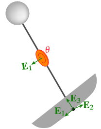
Figure 3. Pendulum skate controlled by an internal rotor attached to the center of mass. Its axis of rotation is aligned with $\mathbf{E}_{1}$, i.e., the edge of the skate.

Following [5], let $\mathsf{H}$ be an $s$-dimensional Abelian Lie group and $\mathfrak{h}\cong\mathbb{R}^{s}$ be its Lie algebra; practically $\mathsf{H}$ gives the configuration space of $s$ internal rotors, i.e., $\mathsf{H}=\mathbb{T}^{s}$. We shall replace the reduced Lagrangian (28) by

$$\ell_{\rm r}\colon\mathfrak{g}\times\mathfrak{h}\times X^{*}\to\mathbb{R};\qquad\ell_{\rm r}{\left(\xi,\dot{\theta}^{a},\Gamma\right)}\mathrel{\mathop{:}}=K{\left(\xi,\dot{\theta}^{a}\right)}-U(\Gamma),$$ (43)

where

$$K{\left(\xi,\dot{\theta}^{a}\right)}\mathrel{\mathop{:}}=\frac{1}{2}\mathbb{G}_{ij}\,\xi^{i}\xi^{j}+\mathbb{G}_{ia}\,\xi^{i}\dot{\theta}^{a}+\frac{1}{2}\mathbb{G}_{ab}\,\dot{\theta}^{a}\dot{\theta}^{b}$$

with a constant symmetric kinetic energy tensor $\mathbb{G}$, i.e., $\mathbb{G}_{ba}=\mathbb{G}_{ab}$; also $\mathbb{G}_{ai}$ and $\mathbb{G}_{ia}$, seen as matrices, are transposes to each other.

Then the equations of motion with control inputs (torques) $\{u_{a}\}_{a=1}^{s}$ applied to the $\mathsf{H}$-part (internal rotors) are

$$\dot{p}_{\alpha} =-\mathcal{B}_{\alpha\beta}^{i}(\Gamma)\,p_{i}\,v^{\beta}-K_{\alpha j}^{k}\,\frac{\partial U}{\partial\Gamma_{j}}\Gamma_{k},$$ (44a)

$$\dot{\pi}_{a} =u_{a},$$ (44b)

$$\dot{\Gamma}_{i} =-\varkappa^{k}_{i\beta}(\Gamma)\,v^{\beta}\,\Gamma_{k},$$ (44c)

where $\{p_{i}\}_{i=1}^{n}$ and $\{\pi_{a}\}_{a=1}^{s}$ are (re-)defined as follows using the modified Lagrangian (43):

$$p_{i}\mathrel{\mathop{:}}={\left\langle\left.\frac{\delta\ell_{\rm r}}{\delta\xi}\right|_{\rm c},\mathcal{E}_{i}\right\rangle}=\mathcal{G}_{i\beta}\,v^{\beta}+\mathcal{G}_{ia}\,\dot{\theta}^{a},\qquad\pi_{a}\mathrel{\mathop{:}}=\left.\frac{\partial\ell_{\rm r}}{\partial\dot{\theta}^{a}}\right|_{\rm c}=\mathcal{G}_{a\alpha}\,v^{\alpha}+\mathbb{G}_{ab}\,\dot{\theta}^{b},$$ (45)

where

$$\mathcal{G}_{ia}(\Gamma)\mathrel{\mathop{:}}=\mathcal{E}_{i}^{j}(\Gamma)\,\mathbb{G}_{ja},$$ (46)

and $\mathcal{G}_{ai}$ is the transpose of $\mathcal{G}_{ia}$. Notice that $\mathcal{G}_{ia}$ is slightly different from $\mathcal{G}_{ij}$ defined in (29) and should be distinguished based on the type of indices just like the $\mathbb{G}$’s defined above.

Again following [5], we consider the controlled Lagrangian of the form

$$\tilde{\ell}_{\rm r}{\left(\xi,\dot{\theta}^{a},\Gamma\right)}\mathrel{\mathop{:}}=\tilde{K}{\left(\xi,\dot{\theta}^{a}\right)}-U(\Gamma)$$ (47a)

with

$$\begin{split}\tilde{K}{\left(\xi,\dot{\theta}^{a}\right)}&\mathrel{\mathop{:}}=K{\left(\xi^{i},\dot{\theta}^{a}+\tau^{a}_{i}\,\xi^{i}\right)}+\frac{1}{2}\sigma_{ab}\,\tau^{a}_{i}\tau^{b}_{j}\,\xi^{i}\xi^{j}\\ &\quad+\frac{1}{2}(\rho_{ab}-\mathbb{G}_{ab})\Bigl{(}\dot{\theta}^{a}+(\mathbb{G}^{ac}\mathbb{G}_{ci}+\tau^{a}_{i})\xi^{i}\Bigr{)}\Bigl{(}\dot{\theta}^{b}+(\mathbb{G}^{bc}\mathbb{G}_{cj}+\tau^{b}_{j})\xi^{j}\Bigr{)},\end{split}$$ (47b)

where $\tau^{a}_{i}$, $\sigma_{ab}$, and $\rho_{ab}$ are all constant matrices and the last two are symmetric.

Let us define

$$\begin{split}\tilde{p}_{i}\mathrel{\mathop{:}}={\left\langle\left.\frac{\delta\tilde{\ell}_{\rm r}}{\delta\xi}\right|_{\rm c},\mathcal{E}_{i}\right\rangle}&=\mathcal{G}_{i\alpha}\,v^{\alpha}+\mathcal{G}_{ia}\dot{\theta}^{a}+{\left(\mathcal{G}_{ib}+\sigma_{ab}\,\mathcal{T}^{a}_{i}\right)}\mathcal{T}^{b}_{\alpha}\,v^{\alpha}+\mathbb{G}_{ab}\,\rho^{bc}\,\tilde{\pi}_{c}\,\mathcal{T}^{a}_{i}\\ &\quad+(\rho_{ab}-\mathbb{G}_{ab})\rho^{ad}\,\tilde{\pi}_{d}{\left(\mathbb{G}^{bc}\mathcal{G}_{ci}+\mathcal{T}^{b}_{i}\right)}\end{split}$$ (48)

and

$$\tilde{\pi}_{a}\mathrel{\mathop{:}}=\left.\frac{\partial\tilde{\ell}_{\rm r}}{\partial\dot{\theta}^{a}}\right|_{\rm c}=\left.\rho_{ab}\Bigl{(}\dot{\theta}^{b}+\mathbb{G}^{bc}\mathbb{G}_{ci}\,\xi^{i}+\tau^{b}_{i}\,\xi^{i}\Bigr{)}\right|_{\rm c}=\rho_{ab}\Bigl{(}\dot{\theta}^{b}+\mathbb{G}^{bc}\mathcal{G}_{c\alpha}\,v^{\alpha}+\mathcal{T}^{b}_{\alpha}\,v^{\alpha}\Bigr{)}.$$ (49)

See Section A.2 for the derivation of the expression for $\tilde{p}_{i}$, where we defined

$$\mathcal{T}^{a}_{i}\mathrel{\mathop{:}}=\tau^{a}_{j}\,\mathcal{E}_{i}^{j}.$$ (50)

Then the nonholonomic Euler–Poincaré equations (25) with the controlled Lagrangian $\tilde{\ell}_{\rm r}$ are given by

$$\dot{\tilde{p}}_{\alpha} =-\mathcal{B}_{\alpha\beta}^{i}(\Gamma)\,v^{\beta}\tilde{p}_{i}-K_{\alpha j}^{k}\,\frac{\partial U}{\partial\Gamma_{j}}\Gamma_{k},$$ (51a)

$$\dot{\tilde{\pi}}_{a} =0,$$ (51b)

$$\dot{\Gamma}_{i} =-\varkappa^{k}_{i\beta}(\Gamma)\,v^{\beta}\,\Gamma_{k}.$$ (51c)

6.2. Matching and Control Law

It turns out that the same sufficient condition for matching from [5, Theorem 2.1] works here:

Proposition 13.

The controlled Euler–Poincaré equations (44) and the Euler–Poincaré equations (51) with the (reduced) controlled Lagrangian $\tilde{\ell}_{\rm r}$ coincide if

$$\tau^{a}_{i}=-\sigma^{ab}\mathbb{G}_{bi}\quad\text{and}\quad\sigma^{ab}+\rho^{ab}=\mathbb{G}^{ab}.$$ (52)

Then the resulting control law is

$$u_{a}=\mathbb{G}_{ab}{\left(\mathcal{T}^{b}_{i}\,\mathcal{F}^{i}_{\alpha\beta}\,v^{\alpha}v^{\beta}-\mathcal{T}^{b}_{\alpha}\,\dot{v}^{\alpha}\right)}.$$ (53)

Proof.

See Section A.3. ∎

Remark 14.

One can eliminate the acceleration $\dot{v}^{\alpha}$ from the control law (53) using (44a).

Example 15 (Pendulum skate with a rotor).

Going back to the motivating example from Figure 3, we may write the reduced Lagrangian with a rotor as follows:

$$\begin{split}\ell_{\rm r}&\colon\mathfrak{se}(3)\times T_{1}\mathbb{S}^{1}\times(\mathbb{R}^{3})^{*}\cong\mathbb{R}^{6}\times\mathbb{R}\times\mathbb{R}^{3}\to\mathbb{R};\\ \ell_{\rm r}&{\left(\boldsymbol{\Omega},\mathbf{Y},\dot{\theta},\boldsymbol{\Gamma}\right)}\mathrel{\mathop{:}}=K_{\rm r}{\left(\boldsymbol{\Omega},\mathbf{Y},\dot{\theta}\right)}-m\mathrm{g}l\boldsymbol{\Gamma}^{T}\mathbf{E}_{3}\end{split}$$ (54)

with

$$\begin{split}K_{\rm r}{\left(\boldsymbol{\Omega},\mathbf{Y},\dot{\theta}\right)}&\mathrel{\mathop{:}}=\frac{1}{2}\Bigl{(}(I_{1}+ml^{2})\Omega_{1}^{2}+J_{1}\bigl{(}\Omega_{1}+\dot{\theta}\bigr{)}^{2}+(\mathcal{I}_{2}+ml^{2})\Omega_{2}^{2}+\mathcal{I}_{3}\Omega_{3}^{2}\Bigr{)}\\ &\qquad+ml(\Omega_{2}Y_{1}-\Omega_{1}Y_{2})+m{\left\|\mathbf{Y}\right\|}^{2}\\ &=\frac{1}{2}\Bigl{(}(\mathcal{I}_{1}+ml^{2})\Omega_{1}^{2}+(\mathcal{I}_{2}+ml^{2})\Omega_{2}^{2}+\mathcal{I}_{3}\Omega_{3}^{2}+ml(\Omega_{2}Y_{1}-\Omega_{1}Y_{2})+m{\left\|\mathbf{Y}\right\|}^{2}\Bigr{)}\\ &\qquad+J_{1}\Omega_{1}\dot{\theta}+\frac{1}{2}J_{1}\dot{\theta}^{2},\end{split}$$ (55)

where

$$\mathcal{I}_{i}\mathrel{\mathop{:}}=I_{i}+J_{i}$$

with $J_{i}$ ($i=1,2,3$) being the moments of inertia of the rotor; note that $m$ now denotes the total mass of the system including the rotor. Hence we have

$$\mathbb{G}_{ij}=\begin{bmatrix}\mathcal{I}_{1}+ml^{2}&0&0&0&-ml&0\\ 0&\mathcal{I}_{2}+ml^{2}&0&ml&0&0\\ 0&0&\mathcal{I}_{3}&0&0&0\\ 0&ml&0&m&0&0\\ -ml&0&0&0&m&0\\ 0&0&0&0&0&m\\ \end{bmatrix},\qquad\mathbb{G}_{ia}=\begin{bmatrix}J_{1}\\ 0\\ 0\\ 0\\ 0\\ 0\end{bmatrix}=J_{1}\mathbf{e}_{1},\qquad\mathbb{G}_{ab}=J_{1}.$$

Note that $\sigma_{ab}=\mathrel{\mathop{:}}\sigma$ and $\rho_{ab}=\mathrel{\mathop{:}}\rho$ are all scalars because there is only one internal rotor ($s=1$). Then the matching conditions (52) give

$$\tau^{a}_{i}=-\frac{J_{1}}{\sigma}\,\mathbf{e}_{1}^{T}\iff\mathcal{T}^{a}_{i}=\tau^{a}_{j}\,\mathcal{E}_{i}^{j} =-\frac{J_{1}}{\sigma}\begin{bmatrix}\mathbf{e}_{1}^{T}\mathcal{E}_{1}&\cdots&\mathbf{e}_{1}^{T}\mathcal{E}_{6}\end{bmatrix}$$

$$=-\frac{J_{1}}{\sigma}\begin{bmatrix}1&\Gamma_{1}&0&0&0&0\end{bmatrix}$$

$$=-\frac{J_{1}}{\sigma}\mathbf{e}_{1}^{T},$$

noting that $\Gamma_{1}=0$, and

$$\frac{1}{\sigma}+\frac{1}{\rho}=\frac{1}{J_{1}}\iff\rho=\frac{J_{1}}{1-J_{1}/\sigma}.$$

Then (53) gives the control law

$$u_{a}=\frac{J_{1}^{2}}{\sigma}\,\dot{v}^{1}=\frac{J_{1}}{\sigma}\,\frac{\Gamma_{2}\bigl{(}m\mathrm{g}l+\left(ml^{2}+I_{2}-I_{3}\right)\Gamma_{3}(v^{2})^{2}\bigr{)}+ml\Gamma_{3}v^{2}v^{3}}{(I_{1}+ml^{2})/J_{1}},$$ (56)

which is what we obtained in [11, Eq. (15d)] (with $\sigma=-J_{1}/\nu$) using a simpler and ad-hoc controlled Lagrangian.

Let us find the controlled Lagrangian. First, again using $\Gamma_{1}=0$,

$$\mathcal{G}_{ai}=\mathbb{G}_{aj}\mathcal{E}_{i}^{j}\,=J_{1}\mathbf{e}_{1}^{T}\mathcal{E}_{i}^{T}=J_{1}\begin{bmatrix}1&\Gamma_{1}&0&\dots&0\end{bmatrix}=J_{1}\mathbf{e}_{1}^{T}.$$

Then (49) gives

$$\tilde{\pi}_{a}=J_{1}v^{1}+\frac{J_{1}}{1-J_{1}/\sigma}\dot{\theta}.$$

Since $\tilde{\pi}_{a}$ is conserved according to (51b), we impose that

$$\tilde{\pi}_{a}=0\iff\dot{\theta}={\left(\frac{J_{1}}{\sigma}-1\right)}v^{1}={\left(\frac{J_{1}}{\sigma}-1\right)}\Omega_{1},$$

and substitute it to (47) to obtain

$$\tilde{\ell}_{\rm r}{\left(\boldsymbol{\Omega},\mathbf{Y},{\left(\frac{J_{1}}{\sigma}-1\right)}\Omega_{1},\Gamma\right)}=\frac{1}{2}\boldsymbol{\Omega}^{T}\tilde{\mathbb{I}}\boldsymbol{\Omega}+\frac{m}{2}{\left\|\mathbf{Y}+l\boldsymbol{\Omega}\times\mathbf{E}_{3}\right\|}^{2}-m\mathrm{g}l\boldsymbol{\Gamma}^{T}\mathbf{E}_{3},$$

where

$$\tilde{\mathbb{I}}\mathrel{\mathop{:}}=\operatorname{diag}{\left(I_{1}+\frac{J_{1}^{2}}{\sigma},\,I_{2}+J_{2},\,I_{3}+J_{3}\right)}.$$ (57)

Notice that this controlled Lagrangian takes the same form as the Lagrangian (7) of the original pendulum skate without the rotor, with the only difference being the inertia tensors $\mathbb{I}$ and $\tilde{\mathbb{I}}$.

7. Stabilization of Pendulum Skate

7.1. Stabilization of Sliding Equilibrium

Recall from Proposition 12 that the sliding equilibrium (40) was always unstable without control. The control law obtained above using the controlled Lagrangian can stabilize it:

Proposition 16.

The sliding equilibrium (40) of the pendulum skate with an internal rotor from Figure 3 is stable with the control (56) if

$$-\frac{J_{1}^{2}}{I_{1}+ml^{2}}<\sigma<0.$$ (58)

Proof.

See Section A.4. ∎

Remark 17.

In terms of $\nu\mathrel{\mathop{:}}=-J_{1}/\sigma$, the control gain in view of (56), the above condition (58) is equivalent to $\nu>(I_{1}+ml^{2})/J_{1}$, which is what we had in [11, Eq. (18) in Theorem 4].

7.2. Numerical Results—Uncontrolled

As a numerical example, consider the pendulum skate with $m=2.00\,[\text{kg}]$, $l=0.80\,[\text{m}]$, $(I_{1},I_{2},I_{3})=(0.35,0.35,0.004)\,[\text{kg}\cdot\text{m}^{2}]$ with $\mathrm{g}=9.80\,[\text{m}/\text{s}^{2}]$. As the initial condition, we consider a small perturbation to the sliding equilibrium (40):

$$\begin{array}[]{c}\boldsymbol{\Omega}(0)=(0.1,\,0.1\tan\phi_{0},\,0.1),\qquad\mathbf{Y}(0)=(1,0,0),\qquad\boldsymbol{\Gamma}(0)=(0,\sin\phi_{0},\cos\phi_{0}),\end{array}$$ (59)

where $\phi_{0}=0.1$ is the small angle of tilt of the pendulum skate away from the vertical upward direction. Figure 4 shows the result of the simulation of the uncontrolled pendulum skate (35) with the above initial condition. It clearly exhibits instability as the pendulum skate falls down.

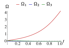
(a) Body angular velocity $\boldsymbol{\Omega}$

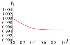
(b) Velocity $Y_{1}$ in body frame

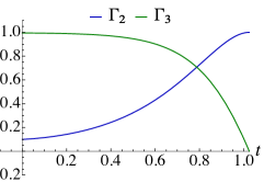
(c) Vertical upward direction $\boldsymbol{\Gamma}$ seen from body frame

Figure 4. Numerical results for the uncontrolled pendulum skate (35) with $m=2.00\,[\text{kg}]$, $l=0.80\,[\text{m}]$, $(I_{1},I_{2},I_{3})=(0.35,0.35,0.004)\,[\text{kg}\cdot\text{m}^{2}]$. The initial condition (59) is a small perturbation from the sliding equilibrium (40). The pendulum skate falls down, i.e., $\Gamma_{3}=0$ at $t\simeq 1.025$ exhibiting the instability of the sliding equilibrium shown in Proposition 12.

7.3. Numerical Results—Controlled

We also solved the controlled system  (44) (see also Example 15) with the control (56) using the same initial condition (59). The mass of the rotor is $1\,[\text{kg}]$, making the total mass $m=3\,[\text{kg}]$; we also set $(J_{1},J_{2},J_{3})=(0.005,0.0025,0.0025)\,[\text{kg}\cdot\text{m}^{2}]$. The lower bound for $\sigma$ shown in (58) in order to achieve stability is $-J_{1}^{2}/(I_{1}+ml^{2})\simeq-1.10\times 10^{-5}$; hence we set $\sigma=-10^{-5}$ here. Figure 5 shows that the system is indeed stabilized by the control.

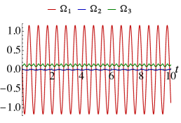
(a) Body angular velocity $\boldsymbol{\Omega}$

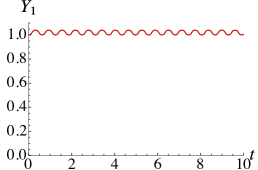
(b) Velocity $Y_{1}$ in body frame

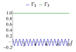
(c) Vertical upward direction $\boldsymbol{\Gamma}$ seen from body frame

Figure 5. Numerical results for the controlled pendulum skate (44) (see also Example 15) with $m=3.00\,[\text{kg}]$, $(J_{1},J_{2},J_{3})=(0.005,0.0025,0.0025)\,[\text{kg}\cdot\text{m}^{2}]$. The solutions are shown for the time interval $0\leq t\leq 10$. One sees that the system is stabilized by the control in comparison to Figure 4; particularly, $\Gamma_{3}$ stays close to 1, indicating that it maintains its position almost upright.

Appendix A Some Proofs

A.1. Proof of Proposition 11

The Jacobin $Df$ of the vector field $f$ from (38) at the spinning equilibrium (41) is

$$Df(\zeta_{\rm sp})=\begin{bmatrix}0&0&\frac{ml\Omega_{0}}{I_{1}+ml^{2}}&\frac{m\mathrm{g}l-\left(I_{3}+ml^{2}-I_{2}\right)\Omega_{0}^{2}}{I_{1}+ml^{2}}&0\\ 0&0&0&0&0\\ -2l\Omega_{0}&0&0&0&0\\ 1&0&0&0&0\\ 0&0&0&0&0\end{bmatrix},$$

and its eigenvalues are

$$\left\{0,0,0,\pm\sqrt{\frac{m\mathrm{g}l-(I_{3}+ml^{2}-I_{2})\Omega_{0}^{2}}{I_{1}+ml^{2}}}\right\}.$$

If $I_{3}+ml^{2}<I_{2}$ then by the Instability from Linearization criterion (see, e.g., Sastry [19, p.216]), $\zeta_{\rm sp}$ is unstable. On the other hand, if $I_{3}+ml^{2}>I_{2}$ then the linear analysis is inconclusive, and so we would like to use the following nonlinear method:

Energy–Casimir Theorem (Aeyels [1]).

Consider a system of differential equations $\dot{\zeta}=f(\zeta)$ on ${\mathbb{R}}^{n}$ with locally Lipschitz $f\colon\mathbb{R}^{n}\to\mathbb{R}^{n}$ with an equilibrium $\zeta_{0}\in\mathbb{R}^{n}$, i.e., $f(\zeta_{0})=0$. Assume that the system has $k+1(<n)$ invariants $\mathscr{E}$ and $\{C_{j}\}_{j=1}^{k}$ that are $C^{2}$ and submersive at $\zeta_{0}$, and also that the gradients $\{DC_{j}(\zeta_{0})\}_{j=1}^{k}$ at $\zeta_{0}$ are linearly independent. Then $\zeta_{0}$ is a stable equilibrium if

1. there exist scalars $\{c_{j}\in\mathbb{R}\}_{j=1}^{k}$ such that $D(\mathscr{E}+c_{1}C_{1}+\dots+c_{k}C_{k})(\zeta_{0})=0$; and

2. the Hessian $\mathscr{H}\mathrel{\mathop{:}}=D^{2}(\mathscr{E}+c_{1}C_{1}+\dots+c_{k}C_{k})(\zeta_{0})$ is sign definite on the tangent space at $\zeta_{0}$ of the submanifold ${\left\{\zeta\in\mathbb{R}^{n}\ |\ C_{j}(\zeta)=C_{j}(\zeta_{0})\ \forall j\in\{1,\dots,k\}\right\}}$, i.e., for any $w\in{\mathbb{R}}^{n}\backslash\{0\}$ satisfying $DC_{j}(\zeta_{0})\cdot w=0$ with every $j\in\{1,\dots,k\}$, one has $w^{T}\mathscr{H}w>0$ (or $<0$).

We note that, despite its name, the above theorem does not assume that the invariants are Casimirs: any invariants—Casimirs or not—would suffice.

In order to use the above theorem, we set the constrained energy (30) as $\mathscr{E}$ and use the invariants $C_{1}$ and $C_{2}$ from (36) and (37) as well as $C_{3}=(\Gamma_{2}^{2}+\Gamma_{3}^{2})/2$ with $k=3$. Now, since

$$D\mathscr{E}(\zeta_{\rm sp})=\begin{bmatrix}0\\ I_{3}\Omega_{0}\\ 0\\ 0\\ I_{3}\Omega_{0}^{2}+m\mathrm{g}l\end{bmatrix},\quad DC_{1}(\zeta_{\rm sp})=\begin{bmatrix}0\\ I_{3}\\ 0\\ 0\\ 2I_{3}\Omega_{0}\end{bmatrix},\quad DC_{2}(\zeta_{\rm sp})=\begin{bmatrix}0\\ 0\\ 1\\ 2l\Omega_{0}\\ 0\end{bmatrix},\quad DC_{3}(\zeta_{\rm sp})=\begin{bmatrix}0\\ 0\\ 0\\ 0\\ 1\end{bmatrix},$$

setting $(c_{1},c_{2},c_{3})=(-\Omega_{0},0,I_{3}\Omega_{0}^{2}-m\mathrm{g}l)$, we have

$$D(\mathscr{E}+c_{1}C_{1}+c_{2}C_{2}+c_{3}C_{3})(\zeta_{\rm sp})=0.$$

Then we also see that

$$\mathscr{H} \mathrel{\mathop{:}}=D^{2}(\mathscr{E}+c_{1}C_{1}+c_{2}C_{2}+c_{3}C_{3})(\zeta_{\rm sp})$$

$$=\begin{bmatrix}I_{1}+ml^{2}&0&0&0&0\\ 0&I_{3}&0&0&0\\ 0&0&m&ml\Omega_{0}&0\\ 0&0&ml\Omega_{0}&\Omega_{0}^{2}\left(I_{3}+ml^{2}-I_{2}\right)-m\mathrm{g}l&0\\ 0&0&0&0&-m\mathrm{g}l\\ \end{bmatrix}.$$

The relevant tangent space is the null space

$$\ker\begin{bmatrix}DC_{1}(\zeta_{\rm sp})^{T}\\ DC_{2}(\zeta_{\rm sp})^{T}\\ DC_{3}(\zeta_{\rm sp})^{T}\end{bmatrix}={\left\{w=s_{1}\begin{bmatrix}1\\ 0\\ 0\\ 0\\ 0\end{bmatrix}+s_{2}\begin{bmatrix}0\\ 0\\ 0\\ 1\\ 0\end{bmatrix}\ |\ s_{1},s_{2}\in\mathbb{R}\right\}}.$$

Hence we have the quadratic form

$$w^{T}\mathscr{H}w=(I_{1}+ml^{2})s_{1}^{2}+{\left((I_{3}+ml^{2}-I_{2})\Omega_{0}^{2}-m\mathrm{g}l\right)}s_{2}^{2},$$

which is positive definite in $(s_{1},s_{2})$ under the assumed conditions (42).

A.2. Derivation of (48)

We can obtain the expression for $\tilde{p}_{i}$ in (48) as follows: Let us first rewrite its definition as

$$\tilde{p}_{i}\mathrel{\mathop{:}}={\left\langle\left.\frac{\delta\tilde{\ell}_{\rm r}}{\delta\xi}\right|_{\rm c},\mathcal{E}_{i}\right\rangle}=\mathcal{E}_{i}^{j}(\Gamma)\,{\left\langle\left.\frac{\delta\tilde{\ell}_{\rm r}}{\delta\xi}\right|_{\rm c},E_{j}\right\rangle}.$$

Performing the same computations as in [5, Eq. (16)] and using $\xi^{k}=\mathcal{E}^{k}_{l}\,v^{l}$, one has

$${\left\langle\frac{\delta\tilde{\ell}_{\rm r}}{\delta\xi},E_{j}\right\rangle} =\mathbb{G}_{jk}\,\xi^{k}+\mathbb{G}_{ja}{\left(\dot{\theta}^{a}+\tau^{a}_{k}\,\xi^{k}\right)}+\mathbb{G}_{ab}\,\rho^{bc}\,\frac{\partial\tilde{\ell}_{\rm r}}{\partial\dot{\theta}^{c}}\,\tau^{a}_{j}$$

$$\quad+\sigma_{ab}\,\tau^{a}_{j}\tau^{b}_{k}\,\xi^{k}+(\rho_{ab}-\mathbb{G}_{ab})\rho^{ad}\,\frac{\partial\tilde{\ell}_{\rm r}}{\partial\dot{\theta}^{d}}{\left(\mathbb{G}^{bc}\mathbb{G}_{cj}+\tau^{b}_{j}\right)}$$

$$=\mathbb{G}_{jk}\,\mathcal{E}^{k}_{l}v^{l}+\mathbb{G}_{ja}{\left(\dot{\theta}^{a}+\tau^{a}_{k}\,\mathcal{E}^{k}_{l}\,v^{l}\right)}+\mathbb{G}_{ab}\,\rho^{bc}\,\frac{\partial\tilde{\ell}_{\rm r}}{\partial\dot{\theta}^{c}}\,\tau^{a}_{j}$$

$$\quad+\sigma_{ab}\,\tau^{a}_{j}\tau^{b}_{k}\,\mathcal{E}^{k}_{l}\,v^{l}+(\rho_{ab}-\mathbb{G}_{ab})\rho^{ad}\,\frac{\partial\tilde{\ell}_{\rm r}}{\partial\dot{\theta}^{d}}{\left(\mathbb{G}^{bc}\mathbb{G}_{cj}+\tau^{b}_{j}\right)},$$

and so

$$\tilde{p}_{i} =\mathcal{E}_{i}^{j}\biggl{(}\mathbb{G}_{jk}\,\mathcal{E}^{k}_{l}v^{l}+\mathbb{G}_{ja}{\left(\dot{\theta}^{a}+\tau^{a}_{k}\,\mathcal{E}^{k}_{l}\,v^{l}\right)}+\mathbb{G}_{ab}\,\rho^{bc}\,\frac{\partial\tilde{\ell}_{\rm r}}{\partial\dot{\theta}^{c}}\,\tau^{a}_{j}$$

$$\quad\qquad+\sigma_{ab}\,\tau^{a}_{j}\tau^{b}_{k}\,\mathcal{E}^{k}_{l}\,v^{l}+(\rho_{ab}-\mathbb{G}_{ab})\rho^{ad}\,\frac{\partial\tilde{\ell}_{\rm r}}{\partial\dot{\theta}^{d}}{\left(\mathbb{G}^{bc}\mathbb{G}_{cj}+\tau^{b}_{j}\right)}\biggr{)}\biggr{|}_{\rm c}$$

$$=\mathcal{G}_{i\alpha}\,v^{\alpha}+\mathcal{G}_{ia}{\left(\dot{\theta}^{a}+\mathcal{T}^{a}_{\alpha}\,v^{\alpha}\right)}+\mathbb{G}_{ab}\,\rho^{bc}\,\tilde{\pi}_{c}\,\mathcal{T}^{a}_{i}$$

$$\quad+\sigma_{ab}\,\mathcal{T}^{a}_{i}\mathcal{T}^{b}_{\alpha}\,v^{\alpha}+(\rho_{ab}-\mathbb{G}_{ab})\rho^{ad}\,\tilde{\pi}_{d}{\left(\mathbb{G}^{bc}\mathcal{G}_{ci}+\mathcal{T}^{b}_{i}\right)},$$

where we used (49).

A.3. Proof of Proposition 13

One can obtain the matching conditions (52) almost the same way as in the proof of [5, Theorem 2.1]. Indeed, the controlled Euler–Poincaré equations (44) and the Euler–Poincaré equations (51) with the (reduced) controlled Lagrangian $\tilde{\ell}_{\rm r}$ match if $p_{i}$ in (45) and $\tilde{p}_{i}$ in (48) are equal, i.e.,

$${\left(\mathcal{G}_{ib}+\sigma_{ab}\,\mathcal{T}^{a}_{i}\right)}\mathcal{T}^{b}_{\alpha}\,v^{\alpha}+\mathbb{G}_{ab}\,\rho^{bc}\,\tilde{\pi}_{c}\,\mathcal{T}^{a}_{i}+(\rho_{ab}-\mathbb{G}_{ab})\rho^{ad}\,\tilde{\pi}_{d}{\left(\mathbb{G}^{bc}\mathcal{G}_{ci}+\mathcal{T}^{b}_{i}\right)}=0.$$

Let us assume $\mathcal{T}^{a}_{i}=-\sigma^{ab}\mathcal{G}_{bi}$, which is equivalent to to the first matching condition in (52) using the definitions (46) and (50) of $\mathcal{G}_{ai}$ and $\mathcal{T}^{a}_{i}$. Substituting $\mathcal{T}^{a}_{i}=-\sigma^{ab}\mathcal{G}_{bi}$ into the above displayed equation, we obtain

$$\mathcal{G}_{ai}=\rho_{ab}(\mathbb{G}^{bc}-\sigma^{bc})\mathcal{G}_{ci},$$

but then this is satisfied if we assume the second matching condition in (52).

For the control law, we again mimic [5, Section 2.2] as follows: Notice from (45) and (49) that

$$\pi_{a}-\mathbb{G}_{ab}\,\rho^{bd}\,\tilde{\pi}_{d}=-\mathbb{G}_{ab}\,\mathcal{T}^{b}_{\alpha}\,v^{\alpha}.$$

Using (44b), (51b), and the above equality, we have

$$u_{a} =\frac{d}{dt}{\left(\pi_{a}-\mathbb{G}_{ab}\,\rho^{bd}\,\tilde{\pi}_{d}\right)}$$

$$=-\mathbb{G}_{ab}\,\frac{d}{dt}{\left(\mathcal{T}^{b}_{\alpha}\,v^{\alpha}\right)}$$

$$=-\mathbb{G}_{ab}\,\frac{d}{dt}{\left(\tau^{b}_{j}\,\mathcal{E}_{\alpha}^{j}\,v^{\alpha}\right)}$$

$$=-\mathbb{G}_{ab}\,\tau^{b}_{j}\,{\left(D^{k}\mathcal{E}_{\alpha}^{j}\,\dot{\Gamma}_{k}\,v^{\alpha}+\mathcal{E}_{\alpha}^{j}\,\dot{v}^{\alpha}\right)}$$

$$=\mathbb{G}_{ab}\,\tau^{b}_{j}\,{\left(D^{k}\mathcal{E}_{\alpha}^{j}\,\varkappa^{l}_{k\beta}\,\Gamma_{l}\,v^{\alpha}v^{\beta}-\mathcal{E}_{\alpha}^{j}\,\dot{v}^{\alpha}\right)}$$

$$=\mathbb{G}_{ab}\,\tau^{b}_{j}\,{\left(\mathcal{E}_{i}^{j}\,\mathcal{F}^{i}_{\alpha\beta}\,v^{\alpha}v^{\beta}-\mathcal{E}_{\alpha}^{j}\,\dot{v}^{\alpha}\right)}$$

$$=\mathbb{G}_{ab}\,{\left(\mathcal{T}^{b}_{i}\,\mathcal{F}^{i}_{\alpha\beta}\,v^{\alpha}v^{\beta}-\mathcal{T}^{b}_{\alpha}\,\dot{v}^{\alpha}\right)},$$

where we used (51b) and the definitions of $\mathcal{F}$ and $\mathcal{T}$ from (27) and (50) in the third last three equalities.

A.4. Proof of Proposition 16

We employ the same Energy–Casimir method from Section A.1.

Recall from Example 15 that the controlled system is equivalent to the original system (38) whose inertia tensor $\mathbb{I}=\operatorname{diag}(I_{1},I_{2},I_{3})$ is replaced by $\tilde{\mathbb{I}}$ shown in (57):

$$(I_{1},I_{2},I_{3})\to{\left(I_{1}+\frac{J_{1}^{2}}{\sigma},\,I_{2}+J_{2},\,I_{3}+J_{3}\right)}.$$

Therefore, the controlled system possesses invariants $\tilde{\mathscr{E}}$ and $\{\tilde{C}_{i}\}_{i=1}^{3}$ defined by making the above replacement in $\mathscr{E}$ and $\{C_{i}\}_{i=1}^{3}$ (see (30), (36), and (37)); note that $\tilde{C}_{3}=C_{3}=(\Gamma_{2}^{2}+\Gamma_{3}^{2})/2$ because it does not depend on $(I_{1},I_{2},I_{3})$. More specifically, we have

$$D\tilde{\mathscr{E}}(\zeta_{\rm sl})=\begin{bmatrix}0\\ 0\\ mY_{0}\\ 0\\ m\mathrm{g}l\end{bmatrix},\quad D\tilde{C}_{1}(\zeta_{\rm sl})=\begin{bmatrix}0\\ I_{3}+J_{3}\\ 0\\ 0\\ 0\end{bmatrix},\quad D\tilde{C}_{2}(\zeta_{\rm sl})=\begin{bmatrix}0\\ 0\\ 1\\ 0\\ 0\end{bmatrix},\quad D\tilde{C}_{3}(\zeta_{\rm sl})=\begin{bmatrix}0\\ 0\\ 0\\ 0\\ 1\end{bmatrix}.$$

Setting $(c_{1},c_{2},c_{3})=(0,-mY_{0},-m\mathrm{g}l)$, we have

$$D{\left(\tilde{\mathscr{E}}+c_{1}\tilde{C}_{1}+c_{2}\tilde{C}_{2}+c_{3}\tilde{C}_{3}\right)}(\zeta_{\rm sl})=0.$$

Then we also see that

$$\mathscr{H} \mathrel{\mathop{:}}=D^{2}{\left(\tilde{\mathscr{E}}+c_{1}\tilde{C}_{1}+c_{2}\tilde{C}_{2}+c_{3}\tilde{C}_{3}\right)}(\zeta_{\rm sl})$$

$$=\begin{bmatrix}I_{1}+ml^{2}+J_{1}^{2}/\sigma&0&0&0&0\\ 0&I_{3}+J_{3}&0&-mlY_{0}&0\\ 0&0&m&0&0\\ 0&-mlY_{0}&0&-m\mathrm{g}l&0\\ 0&0&0&0&-m\mathrm{g}l\\ \end{bmatrix}.$$

The relevant tangent space is the null space

$$\ker\begin{bmatrix}D\tilde{C}_{1}(\zeta_{\rm sl})^{T}\\ D\tilde{C}_{2}(\zeta_{\rm sl})^{T}\\ D\tilde{C}_{3}(\zeta_{\rm sl})^{T}\end{bmatrix}={\left\{w=s_{1}\begin{bmatrix}1\\ 0\\ 0\\ 0\\ 0\end{bmatrix}+s_{2}\begin{bmatrix}0\\ 0\\ 0\\ 1\\ 0\end{bmatrix}\ |\ s_{1},s_{2}\in\mathbb{R}\right\}}.$$

Hence we have the quadratic form

$$w^{T}\mathscr{H}w={\left(I_{1}+ml^{2}+\frac{J_{1}^{2}}{\sigma}\right)}s_{1}^{2}-m\mathrm{g}l\,s_{2}^{2},$$

which is negative definite in $(s_{1},s_{2})$ under the assumed condition (58).

References

- Aeyels [1992] D. Aeyels. On stabilization by means of the Energy–Casimir method. Systems & Control Letters, 18(5):325–328, 1992.
- Ball et al. [2012] K. R. Ball, D. V. Zenkov, and A. M. Bloch. Variational structures for Hamel’s equations and stabilization. In 4th IFAC Workshop on Lagrangian and Hamiltonian Methods for Non Linear Control, volume 45, pages 178–183, 2012.
- Bloch et al. [2001] A. M. Bloch, N. E. Leonard, and J. E. Marsden. Controlled Lagrangians and the stabilization of Euler–Poincaré mechanical systems. International Journal of Robust and Nonlinear Control, 11(3):191–214, 2001.
- Bloch et al. [2009] A. M. Bloch, J. E. Marsden, and D. V. Zenkov. Quasivelocities and symmetries in non-holonomic systems. Dynamical Systems: An International Journal, 24(2):187–222, 2009.
- Bloch et al. [Dec 2000] A. M. Bloch, N. E. Leonard, and J. E. Marsden. Controlled Lagrangians and the stabilization of mechanical systems. I. The first matching theorem. IEEE Transactions on Automatic Control, 45(12):2253–2270, Dec 2000.
- Burkhardt and Burdick [2016] M. Burkhardt and J. W. Burdick. Reduced dynamical equations for barycentric spherical robots. In 2016 IEEE International Conference on Robotics and Automation (ICRA), pages 2725–2732, 2016.
- Burkhardt [2018] M. R. Burkhardt. Dynamic Modeling and Control of Spherical Robots. PhD thesis, California Institute of Technology, 2018.
- Cendra et al. [1998] H. Cendra, D. D. Holm, J. E. Marsden, and T. S. Ratiu. Lagrangian reduction, the Euler–Poincaré equations, and semidirect products. Amer. Math. Soc. Transl., 186:1–25, 1998.
- Fedorov and Jovanović [2004] Y. N. Fedorov and B. Jovanović. Nonholonomic LR systems as generalized Chaplygin systems with an invariant measure and flows on homogeneous spaces. Journal of Nonlinear Science, 14(4):341–381, 2004.
- Fedorov and Jovanović [2009] Y. N. Fedorov and B. Jovanović. Hamiltonization of the generalized Veselova LR system. Regular and Chaotic Dynamics, 14(4):495–505, 2009.
- Garcia and Ohsawa [2022] J. S. Garcia and T. Ohsawa. Stabilization of nonholonomic pendulum skate by controlled Lagrangians. In 2022 IEEE 61st Conference on Decision and Control (CDC), pages 1861–1866, 2022.
- Gay-Balmaz and Yoshimura [2015] F. Gay-Balmaz and H. Yoshimura. Dirac reduction for nonholonomic mechanical systems and semidirect products. Advances in Applied Mathematics, 63:131–213, 2015.
- Gzenda and Putkaradze [2020] V. Gzenda and V. Putkaradze. Integrability and chaos in figure skating. Journal of Nonlinear Science, 30(3):831–850, 2020.
- Holm [2011] D. D. Holm. Geometric Mechanics, Part II: Rotating, Translating and Rolling. Imperial College Press, 2nd edition, 2011.
- Holm et al. [1998] D. D. Holm, J. E. Marsden, and T. S. Ratiu. The Euler–Poincaré equations and semidirect products with applications to continuum theories. Advances in Mathematics, 137(1):1–81, 1998.
- Holm et al. [2009] D. D. Holm, T. Schmah, and C. Stoica. Geometric mechanics and symmetry: from finite to infinite dimensions. Oxford texts in applied and engineering mathematics. Oxford University Press, 2009.
- Marsden et al. [1984a] J. E. Marsden, T. S. Ratiu, and A. Weinstein. Semidirect products and reduction in mechanics. Transactions of the American Mathematical Society, 281(1):147–177, 1984a.
- Marsden et al. [1984b] J. E. Marsden, T. S. Ratiu, and A. Weinstein. Reduction and Hamiltonian structures on duals of semidirect product Lie algebras. In Fluids and Plasmas : Geometry and Dynamics, volume 28 of Contemporary Mathematics. American Mathematical Society, 1984b.
- Sastry [1999] S. Sastry. Nonlinear Systems: Analysis, Stability, and Control. Interdisciplinary Applied Mathematics. Springer New York, 1999.
- Schneider [2002] D. Schneider. Non-holonomic Euler–Poincaré equations and stability in Chaplygin’s sphere. Dynamical Systems, 17(2):87–130, 2002.
- Tai [2004] M. Tai. Model reduction method for nonholonomic mechanical systems with semidirect product symmetry. In IEEE International Conference on Robotics and Automation, 2004. Proceedings. ICRA ’04. 2004, volume 5, pages 4602–4607 Vol.5, 2004.
- Veselov and Veselova [1986] A. P. Veselov and L. E. Veselova. Currents on Lie groups with nonholonomic connection and integrable nonhamiltonian systems. Functional Analysis and Its Applications, 20(4):308–309, 1986.
- Zenkov [2016] D. V. Zenkov. On Hamel’s equations. Theoretical and Applied Mechanics, 43(2):191–220, 2016.
- Zenkov et al. [2000a] D. V. Zenkov, A. M. Bloch, N. E. Leonard, and J. E. Marsden. Matching and stabilization of low-dimensional nonholonomic systems. In Proceedings of the 39th IEEE Conference on Decision and Control, volume 2, pages 1289–1294 vol.2, 2000a.
- Zenkov et al. [2000b] D. V. Zenkov, A. M. Bloch, N. E. Leonard, and J. E. Marsden. Matching and stabilization of the unicycle with rider. IFAC Proceedings Volumes, 33(2):177–178, 2000b.
- Zenkov et al. [2002a] D. V. Zenkov, A. M. Bloch, and J. E. Marsden. Flat nonholonomic matching. In Proceedings of the 2002 American Control Conference (IEEE Cat. No.CH37301), volume 4, pages 2812–2817 vol.4, 2002a.
- Zenkov et al. [2012] D. V. Zenkov, M. Leok, and A. M. Bloch. Hamel’s formalism and variational integrators on a sphere. In 2012 IEEE 51st IEEE Conference on Decision and Control (CDC), pages 7504–7510, 2012.
- Zenkov et al. [2002b] D. V. Zenkov, A. M. Bloch, and J. E. Marsden. The lyapunov–malkin theorem and stabilization of the unicycle with rider. Systems & Control Letters, 45(4):293–302, 2002b.