AstroSat and NuSTAR observations of XTE J1739$-$285 during the 2019-2020 outburst

Abstract

We report results from a study of XTE J1739$-$285, a transient neutron star low mass X-ray binary observed with AstroSat and NuSTAR during its 2019-2020 outburst. We detected accretion-powered X-ray pulsations at 386 Hz during very short intervals (0.5–1 s) of X-ray flares. These flares were observed during the 2019 observation of XTE J1739$-$285. During this observation, we also observed a correlation between intensity and hardness ratios, suggesting an increase in hardness with the increase in intensity. Moreover, a thermonuclear X-ray burst detected in our AstroSat observation during the 2020 outburst revealed the presence of coherent burst oscillations at 383 Hz during its decay phase. The frequency drift of 3 Hz during X-ray burst can be explained with r modes. Thus, making XTE J1739$-$285 belong to a subset of NS-LMXBs which exhibit both nuclear- and accretion-powered pulsations. The power density spectrum created using the AstroSat-LAXPC observations in 2020 showed the presence of a quasi-periodic oscillation at $\sim 0.83$ Hz. Our X-ray spectroscopy revealed significant changes in the spectra during the 2019 and 2020 outburst. We found a broad iron line emission feature in the X-ray spectrum during the 2020 observation, while this feature was relatively narrow and has a lower equivalent width in 2019, when the source was accreting at higher rates than 2020. Hard X-ray tail was observed during the 2019 observations, indicating the presence of non-thermal component in the X-ray spectra.

1 Introduction

Low-mass X-ray binary (LMXB) systems consist of neutron star (NS) or a black hole (BH) that accretes matter from a low-mass (${\leq}$ 1 ${M_{\sun}}$) companion star via Roche-lobe overflow, forming an accretion disc (Shakura & Sunyaev, 1973). Weakly magnetized, accreting NSs in LMXBs can be spun up to rates of several 100 Hz (Alpar et al., 1982). Accretion-powered millisecond X-ray pulsars (AMXPs) (see e.g., Wijnands & van der Klis, 1998; Wijnands, 2006) and nuclear-powered X-ray millisecond pulsars (NMXPs) (see e.g., Strohmayer et al., 1998, 1999; Strohmayer, 2001) belong to this class of NS-LMXB systems. Till date, only 25 AMXPs (see e.g., Patruno & Watts, 2012; Campana & Di Salvo, 2018; Di Salvo & Sanna, 2020; Bult et al., 2022; Ng et al., 2022) and 19 confirmed NMXPs (see e.g., Galloway et al., 2008; Bhattacharyya, 2021, for a recent review) are known. All these AMXPs are transient in nature which means they spend most of their time in quiescence with X-ray luminosity of $L_{X}\sim 10^{30}-10^{33}$ erg s^-1, interrupted by an occasional outburst episode. For the vast majority of AMXPs, $L_{X}$ during outburst remains below $10{\%}$ the Eddington luminosity (see Table 2 of Marino et al., 2019). No spectral state transitions between hard and soft are often observed during these outbursts (Di Salvo & Sanna, 2020). In NMXPs coherent millisecond period brightness oscillations have been observed during thermonuclear X-ray bursts (sudden eruptions in X-rays, intermittently observed from NS-LMXBs). There also exists a partial overlap between AMXPs and NMXPs which means some AMXPs are also NMXPs, and vice versa (see e.g., Chakrabarty et al., 2003; Strohmayer et al., 2003; Altamirano et al., 2010; Bhattacharyya, 2021).

XTE J1739$-$285 is a transient NS LMXB system, discovered in October 1999 with the Rossi X-ray Timing Explorer (RXTE; Markwardt et al., 1999). This source has displayed irregular outburst patterns. During the 1999 outburst, the $2-10~{}\rm{keV}$ source flux evolved between $1-5~{}{\times}~{}10^{-9}~{}\rm{erg~{}s^{-1}~{}cm^{-2}}$ over a period of roughly two weeks (Markwardt et al., 1999). Bulge scans performed with RXTE-PCA revealed two short and weak outbursts of XTE J1739$-$285 in 2001 and 2003 (Kaaret et al., 2007). In August 2005, the source became active again and was first detected with INTEGRAL at a $3-10~{}\rm{keV}$ flux of $\sim$ 2 ${\times}$ $10^{-9}~{}\rm{erg~{}s^{-1}~{}cm^{-2}}$ (Bodaghee et al., 2005). In about a month the value of flux changed by ten times (Shaw et al., 2005). Further observations made with RXTE between October and November 2005 showed that the flux evolved between $4~{}{\times}~{}10^{-10}$ and 1.5 ${\times}$ $10^{-9}$ $\rm{erg~{}s^{-1}~{}cm^{-2}}$. Moreover, after a period of Solar occultation, XTE J1739$-$285 was still visible in early 2006 (Chenevez et al., 2006). In 2012, the source underwent another outburst (Sanchez-Fernandez et al., 2012). After seven years of a quiet period, the 2019 outburst occurred, which was first detected with INTEGRAL (Mereminskiy & Grebenev, 2019) and was later followed-up with the Neutron Star Interior Composition Explorer (NICER) (Bult et al., 2019). The 2$-$10 keV peak flux was about $5~{}{\times}~{}10^{-9}\rm{erg~{}s^{-1}~{}cm^{-2}}$ as measured with MAXI-GSC during its 2019 outburst (Negoro et al., 2020). Very recently in 2020, XTE J1739$-$285 was again found to be active with INTEGRAL (Sanchez-Fernandez et al., 2020), the rebrightening phase of XTE J1739$-$285 was soon confirmed with Swift (Bozzo et al., 2020), and the source was extensively followed with NICER.

Since its discovery, several X-ray bursts have been found in this source. 43 events have been cataloged in the Multi-Instrument Burst Archive (MINBAR, Galloway et al., 2020), including most detections with JEM-X instrument on INTEGRAL and six with RXTE. Kaaret et al. (2007) found oscillations at 1122 Hz in one of these bursts detected with RXTE, suggesting it to be the fastest spinning neutron star. However, the burst oscillation at 1122 Hz was never confirmed afterwards for the same burst using independent time windows (Galloway et al., 2008; Bilous & Watts, 2019), casting doubts on the previous detection. Very recently, during the rebrightening phase of XTE J1739$-$285 in 2020, NICER detected a total of 32 X-ray bursts (Bult et al., 2020). These authors did not find any evidence of variability near 1122 Hz, and instead found burst oscillations at around 386 Hz in two X-ray bursts. AstroSat also observed two X-ray bursts during the same outburst, but a detailed timing study has not been reported (Chakraborty & Banerjee, 2020).

In this paper, we report our results from AstroSat and NuSTAR observations of XTE J1739$-$285 during its 2019 and 2020 outbursts. We have performed a detailed timing and spectral study of this source.

2 Observations and data analysis

XTE J1739$-$285 was observed with AstroSat and NuSTAR on October 9, 2019 and February 19, 2020, respectively. Table 1 gives the log of observations that have been used in this work. Figure 1 shows the MAXI–GSC lightcurve of XTE J1739$-$285 during the period of 2019–2020. During the 2019 outburst, AstroSat and NuSTAR observations were made close to the peak of the outburst, while during the rebrightening phase in 2020 the source was caught during the early rise. The hardness ratio computed using the MAXI light curves is also shown in the bottom panel of the Figure 1.

Table 1: Log of X-ray observations.

Instrument	OBS ID	Start Time	Stop time	Exposure Time
		yy-mm-dd hh:mm:ss (MJD)	yy-mm-dd hh:mm:ss (MJD)	ks
LAXPC	9000003208 (Obs 1)	2019-10-01 02:08:54 (58757.09)	2019-10-02 04:24:47 (58758.18)	94.5
SXT	9000003208 (Obs 1)	2019-10-01 03:16:54 (58757.18)	2019-10-02 03:52:55 (58758.18)	82
NuSTAR	90501343002 (Obs 1)	2019-10-01 22:46:26 (58757.94)	2019-10-02 21:41:33 (58758.90)	82.5
LAXPC	9000003524 (Obs 2)	2020-02-19 22:45:39 (58898.95)	2020-02-20 23:19:40 (58899.97)	88.5
SXT	9000003524 (Obs 2)	2020-02-19 22:48:26 (58898.95)	2020-02-20 23:19:38 (58899.97)	88.2
NuSTAR	90601307002 (Obs 2)	2020-02-19 09:30:06 (58898.39)	2020-02-20 02:31:47 (58899.10)	61

Figure 1: The top panel shows the 2–20 keV MAXI/GSC light curve of XTE J1739$-$285 during its 2019-2020 outburst. The blue and purple regions represent the time of AstroSat and NuSTAR observations in 2019, respectively, while deep blue and cyan colour show observations in 2020. The red arrow corresponds to the start of the 2019 outburst (MJD 58753.28) as reported in Mereminskiy & Grebenev (2019) while the purple arrow marks the re-brightening phase of XTE J1739$-$285 in 2020 (MJD 58887.39; Sanchez-Fernandez et al., 2020). The hardness ratio is plotted in the bottom panel.

2.1 LAXPC

LAXPC is one of the primary instrument on-board AstroSat. It consists of three co-aligned identical proportional counter detectors, viz. LAXPC10, LAXPC20 and LAXPC30. Each of these work in the energy range of 3$-$80 keV, independently record the arrival time of each photon with a time resolution of $10~{}\mu$s, and has five layers, each with 12 detector cells (for details see, Yadav et al., 2016b; Antia et al., 2017, 2021).

Due to the gain instability caused by the gas leakage, LAXPC10 data were not used while LAXPC30 was switched off during these observations. Therefore, we have used data from LAXPC20 for our work. These data were collected in the Event Analysis mode (EA) which contains the information about the time, channel number and anodeID of each event. LaxpcSoft v3.3 software package was used to extract light curves and spectra. LAXPC has a dead-time of $42~{}\mu$s and the extracted products are dead-time corrected. Background files are generated using the blank sky observations (see, Antia et al., 2017, for details). To minimize contribution of the background in our analysis we have used data from the top layers (L1, L2) (also see, Beri et al., 2019; Sharma et al., 2020; Sharma et al., 2023, for details). Barycentric correction was performed using the tool as1bary. We used the best available position of the source, R.A. (J2000) $=17^{h}39^{m}53.^{s}95$ and Dec. (J2000) $=-28^{\circ}29^{\prime}46.^{\prime\prime}8$ obtained with Chandra (Krauss et al., 2006).

2.2 SXT

The Soft X-ray Telescope (SXT) is a focusing X-ray telescope with CCD in the focal plane that can perform X-ray imaging and spectroscopy in the 0.3$-$7 keV energy range (Singh et al., 2014; Singh et al., 2017; Bhattacharyya et al., 2021). XTE J1739$-$285 was observed in the Photon Counting (PC) mode with SXT (Table 1). Level 1 data were processed with AS1SXTLevel2-1.4b pipeline to produce level 2 clean event files. Events from each orbit were merged using SXT Event Merger Tool (Julia Code). These merged events were used to extract image, light curves and spectra using the ftool task xselect, provided as part of heasoft version 6.29c. A circular region with radius of 15 arcmin centered on the source was used to extract source events. For spectral analysis, we have used the following files provided by the SXT team⁴: background spectrum (SkyBkg_comb_EL3p5_Cl_Rd16p0_v01.pha), spectral redistribution matrix file (sxt_pc_mat_g0to12.rmf). The ancillary response files (ARF) were generated using sxtARFModule using the standard ARF (sxt_pc_excl00_v04_20190608.arf) file provided by the SXT team. The SXT spectra were grouped to have atleast 25 counts/bin.

2.3 NuSTAR

The Nuclear Spectroscopic Telescope Array (NuSTAR; Harrison et al., 2013) consists of two telescopes, which focus X-rays between 3 and 79 keV onto two identical focal planes (FPMA and FPMB). We have used software distributed with heasoft version 6.29c and the latest calibration files (version 20220331) for the NuSTAR data reduction and analysis. The calibrated and screened event files have been generated using the task nupipeline. A circular region of radius 80 arcsec centred at the source position was used to extract source events. Background events were extracted from the source free region. The nuproduct tool was used to generate light curves, spectra, and response files. The spectra were grouped to have a minimum of 25 counts/bin. The FPMA/FPMB light curves were background corrected and averaged using ftool task lcmath.

3 Results

3.1 Timing Results

3.1.1 X-ray Light curves

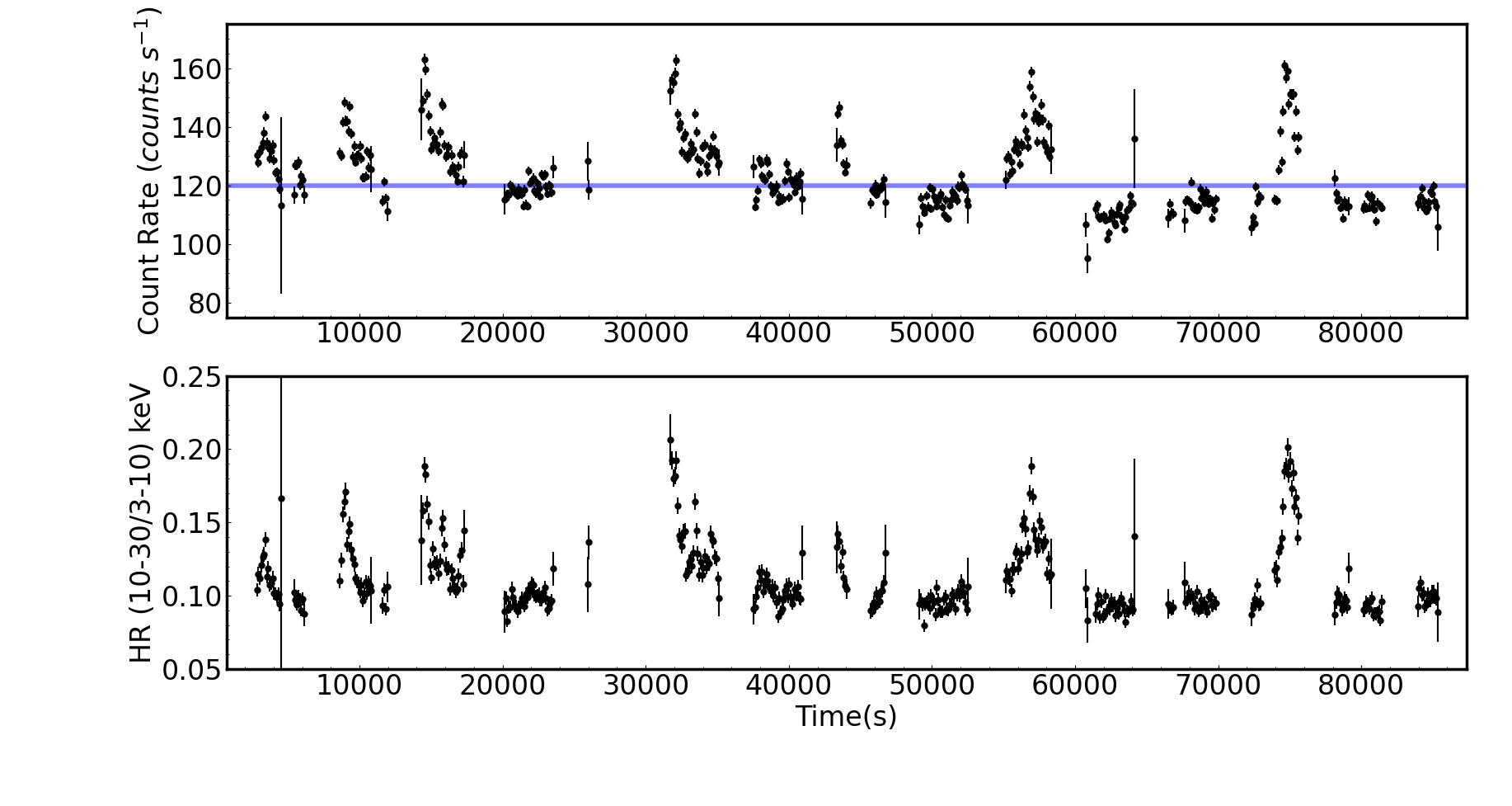
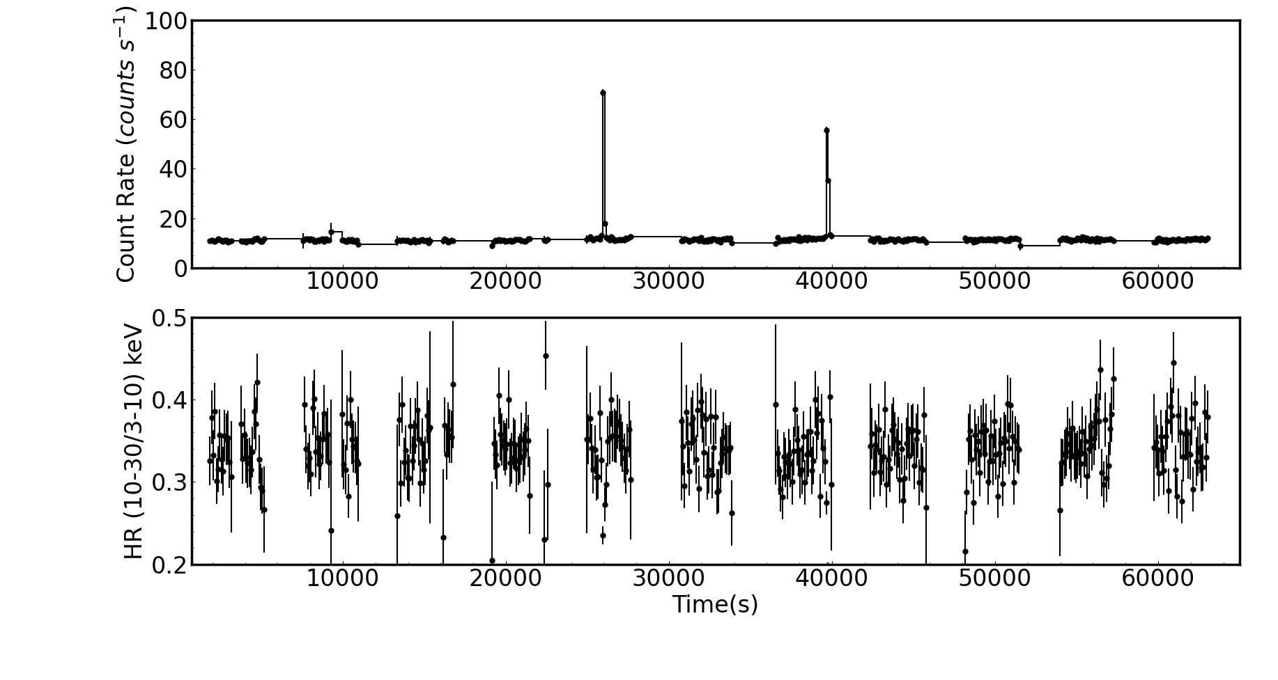
Figure 11: The background corrected light curves of XTE J1739$-$285 obtained from NuSTAR (FPMA) observation of 2019 (left panel) and 2020 (right panel). Both light curves are binned at 100 s and in the energy range of 3–30 keV. The horizontal line in purple show the split of the data based on count rate for performing intensity-resolved spectroscopy (for more details see the text). The bottom panels show the hardness ratio between the count rate in 10-30 keV to 3–10 keV.

Figure 2 shows 3$-$30 keV AstroSat-LAXPC light curves of XTE J1739$-$285 during its observations in 2019 (Obs 1) and 2020 (Obs 2). A large variation in the count rates was observed during the 2019 outburst (left plot of Figure 2). To track spectral evolution during these flares (segments where count rates are varying between 500 and 700 $\rm{count~{}s^{-1}}$), we computed hardness ratio (shown in the bottom panels of Figure 2). HR was computed taking the ratio of count rates in the 10$-$30 keV and 3$-$10 keV energy bands. We observed a correlation between intensity and hardness ratios, suggesting an increase in hardness with the increase in intensity. Similar behaviour was also observed in the NuSTAR light curves (see Figure 11).

On the other hand, LAXPC light curves in 2020 (right plot of Figure 2) showed almost a constant behaviour in the count rates as well as in the hardness ratio. The average count rate estimated is approximately $65~{}\rm{count~{}s^{-1}}$. Moreover, an X-ray burst was also observed during this observation. This is in contrast to that reported by Chakraborty & Banerjee (2020) as we found that the second burst at $\sim 60.7$ ks being filtered out due to the Good Time Interval (GTI) selection. The NuSTAR light curves also showed a constant behaviour (Figure 11) along with the presence of two X-ray bursts. However, X-ray bursts in NuSTAR are not observed at the same time as with AstroSat 

Figure 2: The background corrected light curves of XTE J1739$-$285 obtained from LAXPC20 for the observation of 2019 (left panel) and 2020 (right panel). Both light curves are binned at 20 s and in the energy range of 3–30 keV. The bottom panels present the hardness ratio between the count rate in 10-30 keV energy range to 3–10 keV energy range.

3.1.2 Power Density Spectra

Figure 3: The rms-normalized power density spectrum (white noise subtracted) of XTE J1739$-$285 from the two LAXPC observations. Left panel: PDS from 2019 observation (Obs 1). Right panel: PDS from 2020 observation (Obs 2).

3–30 keV LAXPC light curves created using data from the top layer with a time resolution of 10 ms were used to create the power density spectra (PDS) (shown in Figure 3). We used the ftool task powspec for the purpose. For observations made in 2019 (Obs 1), the PDS could be well-fitted using a single lorentzian. However, to model the PDS created using observations made in 2020 (Obs 2) needed a combination of four Lorentzians components, given individually by,

$$P(\nu)=\frac{r^{2}\Delta}{2\pi}\frac{1}{(\nu-\nu_{0})^{2}+(\Delta/2)^{2}}$$ (1)

where $\nu_{0}$ is the centroid frequency, $\Delta$ is the full-width at half-maximum, and $r$ is the integrated fractional rms (see Belloni et al., 2002). The quality factor (Q) defined as $Q=\nu_{0}/\Delta$ was used to find the presence of a quasi-periodic oscillation (QPO) as $Q~{}\geq~{}3$ indicate the presence of a QPO in the PDS (van der Klis, 1989).

The two lorentzian functions were used to model the band-limited noise while the other two fit QPOs observed (Table 2). One of these QPOs was found at $\sim 0.83$ Hz with $Q\sim 4$ and fractional rms of 7%. This was detected at $9\sigma$ where the significance was calculated by dividing the normalization of Lorentzian function by its negative $1\sigma$ error. We also found a less significant ($\sim 2.7\sigma$) QPO feature at 0.35 Hz with $Q\sim 3.5$ and rms of $\sim 4$%.

Table 2: Fit parameters obtained using 2019 and 2020 observations of LAXPC. Errors quoted are within 90$\%$ confidence range.

Model	parameter	2019	2020
Lorentzian 1	$\nu$ (Hz)	0.01 (fixed)	$0.83\pm 0.01$
	$\Delta$ (Hz)	$0.14\pm 0.02$	$0.20^{+0.04}_{-0.03}$
	rms ($\%$)	$7.3\pm{0.3}$	$6.9\pm{0.4}$
Lorentzian 2	$\nu$ (Hz)	-	$0.35\pm 0.02$
	$\Delta$ (Hz)	-	$0.10^{+0.11}_{-0.07}$
	rms ($\%$)	-	$4.4_{-0.84}^{+4.1}$
Lorentzian 3	$\nu$ (Hz)	-	0
	$\Delta$ (Hz)	-	$3.9^{+0.8}_{-0.5}$
	rms ($\%$)	-	$4.6\pm 0.4$
Lorentzian 4	$\nu$ (Hz)	-	0
	$\Delta$ (Hz)	-	$101^{+23}_{-16}$
	rms ($\%$)	-	$1.8\pm 0.1$

3.1.3 Energy-resolved thermonuclear burst profile

To check energy-dependence of the burst observed in the LAXPC light curves during Obs 2, we created burst profiles in the following energy bands: 3–6 keV, 6–12 keV, 12–18 keV, 18–24 keV and 24–30 keV (see Figure 4). We observed that the burst was significantly detected upto 24 keV. In a few X-ray sources (such as Aql X$-$1, 4U 1728$-$34) a dip has been observed in the hard X-ray light curves during bursts (see Maccarone & Coppi, 2003; Chen et al., 2013; Kajava et al., 2017, for details). Therefore, we investigated the presence of any dip in the 30–80 keV light curves (also see Beri et al., 2019). No dips were found in the hard X-ray light curves during burst. The rise time and exponential decay time measured using the 3-30 keV burst light curve is $4.7\pm 0.1$ s and $11.4\pm 0.3$ s, respectively, consistent with that observed with NICER (Bult et al., 2020).

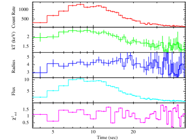
Figure 4: Left panel: Energy-resolved burst profiles from the LAXPC data. Right panel: Time-resolved spectroscopy of the bursts. The burst count rate in 3–20 keV, blackbody temperature in keV, blackbody emission radius in km, absorbed flux ($\times 10^{-9}$ erg cm^-2 s^-1) in 3-20 keV and reduced $\chi^{2}$ for each fit from top to bottom, respectively.

3.1.4 Burst Oscillations (BOs)

We performed a search for <2048 Hz oscillations along the entire duration of each of the burst. Events from only LAXPC20 were taken into account. We performed Fourier transform (FT) of successive $1~{}\rm{s}$ segment (shifting the 1 s time window) of the input barycentre-corrected event file corresponding to the burst time interval. The FT scan was repeated with the start time offset by 0.5 s. While we did not see any signal at $\sim$1122 Hz, a sharp signal at $\sim$383 Hz was clearly seen during the decay phase of the burst in the Leahy-normalized (Leahy et al., 1983) power spectrum (Figure  5). We then examined the region that showed the signal at $\sim$383 Hz and attempted to maximize the measured power, $P_{\text{m}}$, by varying the start and end points of the segment in steps of 0.1 s and trying segment lengths of 1 s, 2 s within a time window of 3 s (20+10=30 overlapping segments). We checked two energy bands: 3$-$10 keV and 3$-$25 keV. The number of trials was thus, $30\times 2=60$. The single-trial chance probability i.e., the probability of obtaining $P_{\text{m}}$ solely due to noise, was then given by the survival function, $e^{-P_{\text{m}}/2}$, where $P_{\text{m}}$ was now the maximized power obtained through the trials. So, the significance was $x=e^{-P_{\text{m}}/2}\times 60$, and the confidence level would be $X\sigma$, where $X=\sqrt{2}erf^{-1}(1-x)$. The signal was detected with $\sim$ 3.4 $\sigma$ ($P_{\text{m}}=23.08$) confidence in a 1 s window during the decay of the burst. The dynamic power spectra on the right side of Figure 5 indicates the presence of a strong signal between 13 and $13.5~{}\rm{s}$ segment.

We also evaluated the significance of the signal using a Monte Carlo simulation that generates Poisson-distributed events following the first 20 s of the burst light curve in 1 s bins. LAXPC deadtime is modelled by removing any event that occurs within 43 $\mu$s after a previous event. The number of events generated in each time bin is greater than the observed counts, so that after the deadtime correction the number of events is identical to that in the actual light curve within Poisson fluctuations. We generate, 10000 trial bursts and calculate successive 1 s FFTs (i.e., 20 FFTs per burst) searching for peaks in the 10-1000 Hz range. The chance probability of occurrence of the observed signal is obtained by counting the fraction of trial bursts with Leahy powers equal to or exceeding 21.6 (i.e., the Leahy power corresponding to a single trial probability of 2e-5). For 3-25 keV light curve simulation, we find 19 bursts which have at least one signal above 21.6 in the frequency range 381-387 Hz. Thus, we estimate the chance probability to be 19/10000 = 1.9${\times}10^{-3}$ which implies a significance of 3.1 $\sigma$ since $X=\sqrt{(}2)*erf^{-1}(1-x)$ where x is the chance probability. For 3-10 keV energy band, we find 21 bursts which have at least one signal above 21.6 in the frequency range 381-387 Hz. The chance probability and significance are, thus, 2.1${\times}10^{-3}$ and 3.1 $\sigma$ respectively. A similar search into the NuSTAR data of two bursts did not yield any significant feature.

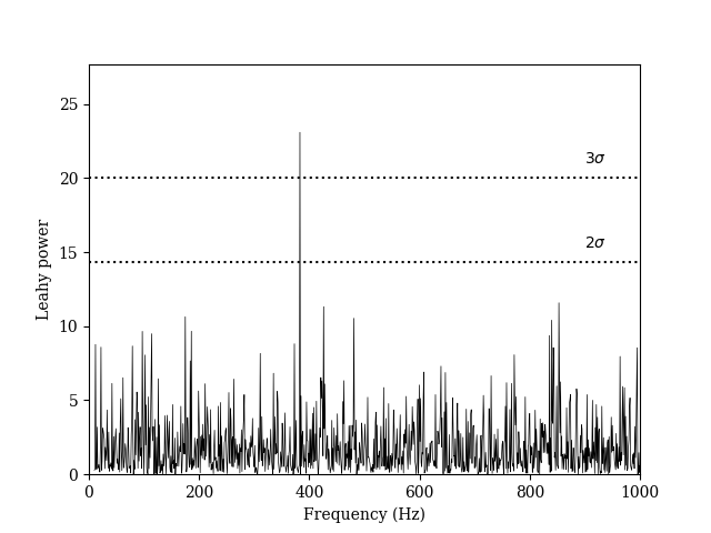
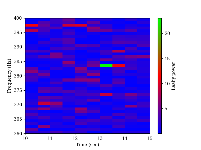
Figure 5: Left panel: Power spectrum for a 1 s window during the decay phase of the 3–10 keV burst, showing burst oscillations at 383 Hz. The sampling rate is 2048 Hz. Right panel: Dynamic power spectra for 5 s window during the decay of the burst.

3.1.5 Search for accretion-powered oscillations during flares

We looked for the presence of $\sim$ 383 Hz signal during the flares in the 3–30 keV LAXPC20 light curves observed during Obs 1, and found a few instances which showed a clear feature at nearby frequencies. Flares during which oscillations were found are shown in the shaded region of left-hand plot in Figure 2. A representative power spectrum with the maximum power and the corresponding dynamic power spectra are shown in Figure 6. The confidence level of this 386 Hz signal detection is estimated to be, $\sim 3.3\sigma$ considering 30 trials.

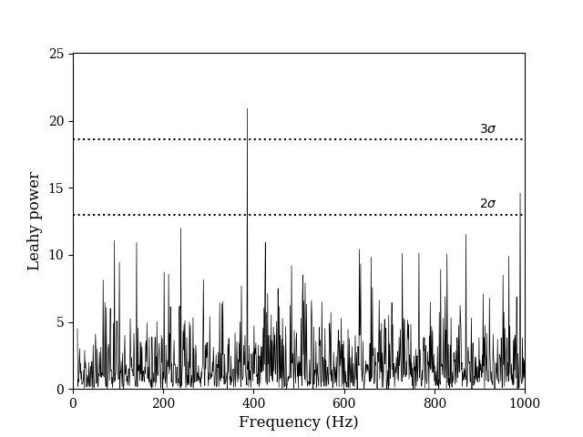
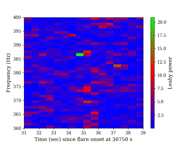
Figure 6: Left panel: Power spectrum for a 1 s window during the flare, showing oscillations at 386 Hz. The sampling rate is 2048 Hz. Right panel: Dynamic power spectra for 8 s window during the same. Each segment is 1 s long and overlaps the previous one by 0.5 s.

3.1.6 X-ray Pulse Profiles

To estimate the fractional amplitude of these oscillations we constructed pulse profiles shown in Figure 7. The phase was determined from the folded pulse profiles modelled with the function $A+B\sin{2\pi\nu t}$. Here, $B/A$ gives the half-fractional amplitude and the fractional amplitude is given by $B/(A\sqrt{2})$. We obtained the fractional amplitude of $29\pm 4\%$ during burst oscillations while during flares it was observed to be $31\pm 4\%$.

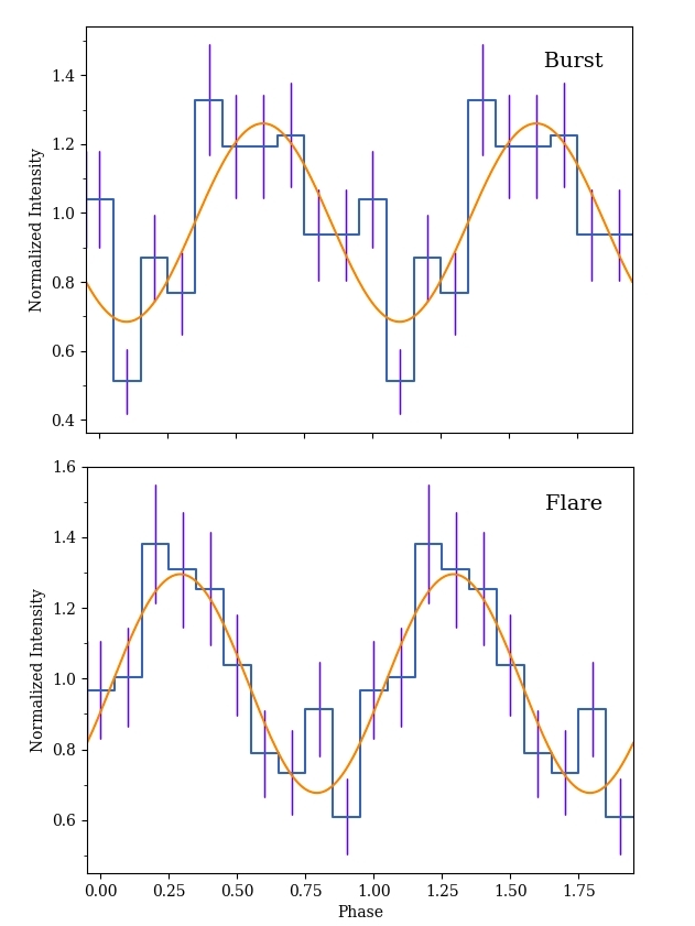
Figure 7: Top panel: Pulse profile in the 3–10 keV band for a 1 s time window during the decay phase of the X-ray burst. The smooth curve shows the sinusoidal fit with frequency 383.14 Hz. The fractional amplitude is $29\pm 4\%$. Bottom panel: Pulse profile in 3–30 keV band for a 1 s time window during the flare. The smooth curve shows the sinusoidal fit with frequency 386.15 Hz. The fractional amplitude is $31\pm 4\%$. In both panels, the second cycle is shown for clarity.

3.2 Spectral results

Table 3: Spectral parameters obtained from the 2019 and 2020 observations.

Model	parameter	2020	2019	2019	2019
			Spectra 1	Spectra 2	Average
tbabs	$N_{\rm H}$ ($10^{22}~{}\rm{cm^{-2}})$	$1.37^{+0.12}_{-0.10}$	$2.3\pm 0.1$	$1.8\pm 0.1$	$2.1\pm 0.1$
bbodyrad	$kT$ (keV)	$1.22^{+0.12}_{-0.19}$	$1.30\pm 0.01$	$1.23\pm 0.01$	$1.23\pm 0.01$
	Norm	$1.17^{+0.79}_{-0.28}$	$68\pm 3$	$100\pm 3$	$100^{+2}_{-5}$
nthcomp	$\Gamma$	$1.75\pm 0.02$	$1.68\pm 0.02$	$1.68\pm 0.02$	$1.68\pm 0.02$
	$kT_{e}$ (keV)	$19.5^{+2.6}_{-1.9}$	$2.95\pm 0.03$	$2.76\pm 0.03$	$2.83\pm 0.03$
	$kT_{\rm seed}$	$0.60\pm 0.05$	$0.21\pm 0.04$	$0.21\pm 0.04$	$0.20\pm 0.04$
	norm	$0.017\pm 0.002$	$0.46\pm 0.07$	$0.30\pm 0.04$	$0.41\pm 0.04$
Gaussian	$E$ (keV)	$6.5\pm 0.2$	$<6.56$	$<6.56$	$<6.56$
	$\sigma$ (keV)	$1.0\pm 0.2$	$0.15^{+0.12}_{-0.15}$	$0.12\pm 0.12$	$0.09_{-0.09}^{+0.21}$
	EqW (keV)	$0.21\pm 0.01$	$0.02\pm 0.01$	$0.02\pm 0.01$	$0.02\pm 0.01$
	norm ($10^{-3}$)	$0.6\pm 0.2$	$0.9_{-0.3}^{+0.5}$	$0.9\pm 0.2$	$0.7\pm 0.3$
powerlaw	$\Gamma$		$0^{\rm fixed}$	$0^{\rm fixed}$	$0^{\rm fixed}$
	Norm ($10^{-6}$)		$3.2\pm 1.5$	$5.8\pm 1.1$	$3.3\pm 0.9$
Cons	$C_{\rm FPMA}$	$1^{\rm fixed}$	$1^{\rm fixed}$	$1^{\rm fixed}$	$1^{\rm fixed}$
	$C_{\rm FPMB}$	$1.034\pm 0.005$	$1.009\pm 0.002$	$1.014\pm 0.002$	$0.982\pm 0.001$
	$C_{\rm SXT}$	$1.21\pm 0.02$	$1.16\pm 0.02$	$1.20\pm 0.02$	$1.09\pm 0.01$
Fluxa	(erg cm-2 s-1)	$8.4\times 10^{-10}$	$6.9\times 10^{-9}$	$6.1\times 10^{-9}$	$6.4\times 10^{-9}$
$L_{X}^{b}$	(erg s-1)	$5.35\times 10^{36}$	$6.0\times 10^{37}$	$5.3\times 10^{37}$	$5.5\times 10^{37}$
	$\chi^{2}$/dof	$2011.8/1975$	$1406/1555$	$1569/1556$	$1375/1681$
aUnabsorbed flux in $0.1-100~{}\rm{keV}$ energy range.
bX-ray luminosity in $0.1-100~{}\rm{keV}$ energy range. Source distance of $7.3~{}\rm{kpc}$ was used.

We performed the spectral fitting using xspec 12.12.0 (Arnaud, 1996). To model the hydrogen column density ($N_{H}$) we have used tbabs using WILM abundances (Wilms et al., 2000). All errors quoted are within 90 $\%$ confidence range.

3.2.1 X-ray spectra during 2019 observations

The LAXPC spectra showed a large calibration uncertainty (Figure 12), with background dominating above $20~{}\rm{keV}$ (see Figure 13). Therefore, we have used a better spectral quality NuSTAR data and contemporaneous SXT data for having energy coverage below $3~{}\rm{keV}$ to perform broadband X-ray spectroscopy. The SXT spectra were corrected for gain offset using the gain fit command with fixed slope of 1.0 and best fit offset of $\sim$ $0.022~{}\rm{eV}$. An offset correction of 0.02$-$0.09 $\rm{keV}$ is needed in quite a few SXT observations (see e.g., Beri et al., 2021). As recommended in the SXT data analysis guide, a systematic error of 2 % was also included in the spectral fits.

As large variation in the count rate as well as the hardness ratio was observed in observations made during the 2019 observations of XTE J1739$-$285  we divided data based on the source count rate (see Figure 11). Two spectra were obtained, one for times when source count rate was $\leq 120$ $count~{}s^{-1}$ (spectra 1) while the other for count rates above this value (spectra 2). FPMA and FPMB spectra were fit simultaneously. A constant model was added to account for flux calibration uncertainties. The value of constant was fixed at 1 for FPMA and was allowed to vary for FPMB and SXT.

We tried to model the continuum emission observed in both these spectra using a physical thermal Comptonized model nthcomp (Zdziarski et al., 1996; Życki et al., 1999). A powerlaw model was used to fit the flat residuals above 40 keV. This returned a value of photon index ($\Gamma$) close to zero, therefore, we fixed its value to 0. The resultant fit showed low energy excess, indicating the presence of thermal emission. Therefore, we added a thermal component bbodyrad. The addition of this model component led to a significant improvement of ${\Delta}{\chi^{2}}$=-2217 and ${\Delta}{\chi^{2}}$=-5441 for 2 degrees of freedom for spectra 1 and spectra 2, respectively. This model (TBabs${\times}$(bbodyrad + nthcomp + po)) fitted the continuum well. The Fe-K_α emission lines at around 6.4 keV have been observed in various neutron star low-mass X-ray binaries and discussed by several authors (see e.g., Bhattacharyya & Strohmayer, 2007; Cackett et al., 2008; Papitto et al., 2009; Sharma et al., 2019; Sharma et al., 2020). Therefore, we added a Gaussian component to model the emission feature observed in the X-ray spectra of XTE J1739-285. The best-fit parameters indicated the presence of a narrow emission feature at around 6.4 keV. Although improvement in the spectral fit was observed ( ${\Delta}{\chi^{2}}$=-33 and ${\Delta}{\chi^{2}}$=-44 for 3 degrees of freedom for spectra 1 and spectra 2), the equivalent width is low. The best fitting parameters are given in Table 3. To evaluate chance probability of improvement of adding the extra Gaussian component, we simulated 100,000 data sets using simftest in xspec. The evaluated chance probability was $<10^{-6}$ for both spectra 1 and 2, rejecting null hypothesis and confirming the presence of an emission feature at 6.4 keV in the spectrum. Since, we did not observe significant differences in the best-fit parameters of Spectra 1 and Spectra 2, we also performed a time-averaged spectroscopy using the same model as described above. Figure 8 shows the SXT and NuSTAR spectrum observed during the 2019 outburst along with the best-fit residuals.

Figure 8: SXT (green) and NuSTAR (FPMA (black) and FPMB (red)) spectrum from observation of 2019. The spectrum were fitted with best fit model. Lower panels show the residuals when absorbed Comptonization model with power-law, thermal and emission component was used, respectively. The residuals show the presence of a narrow emission feature around 6.4 keV in the spectrum. Spectra were rebinned for plotting purpose only.

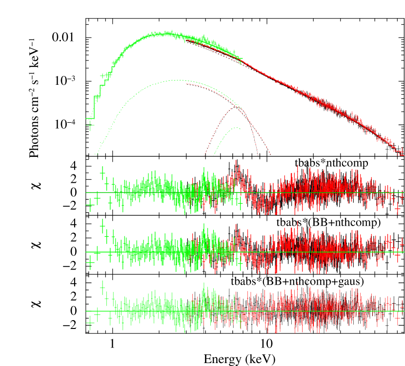
Figure 9: SXT (green) +NuSTAR (FPMA (black) and FPMB (red)) spectrum of observation of 2020. The spectrum can be well-fitted with absorbed blackbody and thermal Comptonization model plus broad Gaussian emission line. Spectra were rebinned for plotting purpose only.

3.2.2 X-ray spectra during 2020 observations

X-ray bursts observed during Obs 2 were removed from the NuSTAR for performing spectroscopy during the persistent emission. No spectral variation was observed, therefore we used the total spectrum (see, Figure 2). Moreover, contemporaneous SXT observation could also be used to account for low energies (0.5–7 keV). The constant model added was kept fixed at 1 for FPMA and was allowed to vary for FPMB and SXT.

The following model: tbabs${\times}$(nthcomp+bbodyrad+Gaussian) best fit the X-ray spectra. In contrast to that observed during the 2019 outburst we did not find hard power law tail in the X-ray spectra. A broad emission feature (Figure 9) was however needed to obtain the best-fit (see Table 3).

3.2.3 Reflection spectrum

We also examined if the broad iron line feature could be better described using the Relativistic reflection model. We fitted the spectra with the self-consistent reflection model relxillCP (Dauser et al., 2014; García et al., 2014). This component includes the thermal Comptonization model nthcomp as the illuminating continuum. To limit the number of the free parameters, we used the single emissivity profile ($r^{-q}$) and fixed emissivity index $q=3$ (Cackett et al., 2010; Wilkins & Fabian, 2012). We fixed the outer radius $R_{\rm out}=1000R_{\rm G}$, where $R_{\rm G}=GM/c^{2}$ is the Gravitational radius. We also fixed The iron abundance $A_{\rm Fe}$ was fixed to 1 in units of solar abundance. The dimensionless spin parameter $a$ can be calculated from the spin frequency using the relation $a$ = 0.47/P[ms] (Braje et al., 2000). Assuming the spin frequency ($\nu$) of 386 Hz, we fixed $a$ at 0.18.

The relxillCP component was added to the nthcomp and fixed the refl_frac to a negative value so that nthcomp represents direct coronal emission component and relxillCP the reflected component. We tied the power-law photon index ($\Gamma$), and electron temperature ($kT_{e}$) of the relxillCP to that of the respective nthcomp parameters. We found an acceptable fit with an absorbed nthcomp+relxillCP model, $\chi^{2}$/dof = 2013.5/1975. We also found that additional thermal component ( bbodyrad or diskbb) was not required. The best-fit parameters obtained are given in Table 4 and the resultant spectrum is shown in Figure  10.

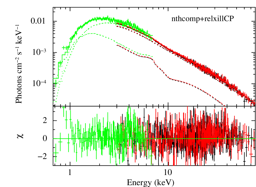
Figure 10: SXT (green)+NuSTAR (FPMA (black) and FPMB (red)) spectrum of XTE J1739$-$285 during the observation of 2020. The spectrum fitted with self- consistent reflection model relxillCP with nthcomp continuum. The figure has been rebinned for representation purpose only.

Table 4: Spectral parameters obtained from the 2020 observations of SXT+NuSTAR.

Model	parameter	value
tbabs	$N_{\rm H}$ ($10^{22}~{}\rm{cm^{-2}}$)	$1.71^{+0.15}_{-0.09}$
nthcomp	$\Gamma$	$1.86^{+0.02}_{-0.01}$
	$kT_{e}$ (keV)	$55.7^{+61.1}_{-10.5}$
	$kT_{\rm seed}$	$0.73\pm 0.03$
	norm	$0.0127^{+0.0007}_{-0.0015}$
relxillCP	$inc$	$39.3^{+19.6}_{-10.7}$
	$R_{\rm in}$ ($R_{\rm ISCO}$)	$3.8^{+5.6}_{-2.0}$
	log $\xi$	$3.30^{+0.15}_{-0.09}$
	norm ($10^{-4}$)	$1.4^{+0.3}_{-0.2}$
Cons	$C_{\rm FPMA}$	$1^{\rm fixed}$
	$C_{\rm FPMB}$	$1.034\pm 0.005$
	$C_{\rm SXT}$	$1.194\pm 0.025$
	$\chi^{2}$/dof	2013.5/1975

3.3 Time-resolved burst spectroscopy

We performed time-resolved spectroscopy using 1 s spectra during the X-ray burst. Each spectrum was modelled using an absorbed blackbody. A pre-burst spectrum extracted from 90 s data segment before the burst was used as a background. The value of $N_{H}$ was fixed to $1.73\times 10^{22}$ cm^-2 (Bult et al., 2020). Results from the time-resolved spectroscopy are shown in the right plot of Figure 4. The top panel shows the variation of count rate in the 3–20 keV energy band. The temperature ($kT$) evolution, blackbody emission radius in unit of km, absorbed flux in units of $10^{-9}$ erg cm^-2 s^-1 in the energy range of 3–20 keV and the reduced $\chi^{2}$ for each fit are plotted from the second to bottom panel, respectively. The blackbody emission radius was calculated from the normalization of bbodyrad, $Norm=R_{\rm km}/D^{2}_{\rm 10kpc}$ and we used source distance of 7.3 kpc (Galloway et al., 2008). A peak temperature and bolometric flux were found to be $2.32\pm 0.09$ keV and, $1.1\times 10^{-8}$ erg cm^-2 s^-1 respectively.

4 Discussion

In this work, we performed a detailed timing and spectral analysis of XTE J1739$-$285 during its 2019-2020 outburst. We discuss our timing and spectral results as follows.

4.1 Timing Behaviour

The X-ray light curves during the 2019 observations (Obs 1 Figure-2) showed a large variability in the count rates which has never been reported earlier from this source. This is in contrast to that observed in the X-ray light curves of Obs 2. Moreover, during observations in 2019, hardness ratio showed an increase with count rates. However, no significant spectral variation was observed during the 2020 observations. The LAXPC light curves showed a single X-ray burst, while two were observed during the NuSTAR observations in 2020 (Obs 2). The energy-resolved X-ray burst light curve with LAXPC indicates that it is significantly detected up to 24 keV (Figure 4). Searching for BOs require an instrument capable of providing ${\mu}{\rm{s}}$ time resolution. After the launch of AstroSat (Singh et al., 2016) and NICER (Arzoumanian et al., 2014) the hunt for BOs began once again. We searched for BOs during the burst and found a peak in the PDS around 383.14 Hz. These oscillations were observed during the decay of the burst at a significance of $3.4\sigma$. Bult et al. (2020) observed similar oscillations at 386 Hz during the rise phase of the burst. A large fractional half-amplitude of the signal measured at $29\pm 4$% (equivalent to a rms amplitude of 21$\pm$3%) was observed, consistent with the NICER measurement (rms amplitude of 26$\pm$4%) during the rising phase (Bult et al., 2020). Although, large value of fractional rms amplitude during the decay phase of an X-ray burst decay has been observed in other sources such as 4U 1636-536 (see e.g., Mahmoodifar et al., 2019; Roy et al., 2021) the mechanism behind this is not clear. Usually decay phase oscillations are explained with surface modes, but the fractional rms amplitude is typically small (about 10$\%$). We could not perform a detailed energy- and phase-resolved analysis due to limited number of counts owing to the unavailability of two other LAXPC detectors.

Since BOs arise due to rotational induced modulation of a brightness asymmetry on the stellar surface, they are believed to closely track the spin frequency of the neutron star (see, e.g. Strohmayer et al., 1996; Chakrabarty et al., 2003; Watts, 2012). Motivated by this and also the fact that there exist an overlap between NMXPs and AMXPs, we searched for $\sim$ 386 Hz oscillations during flares seen in the LAXPC light curves of XTE J1739$-$285 (Obs 1). We found a significant detection at around $\sim$ 386 Hz which strengthened our confidence in the earlier detection of the signal during burst. To our best knowledge, there has been no previous report of an effort of searching for neutron star spin frequency using short segments (1 s) during a flare. It has been found that in AMXPs, coherent X-ray pulsations are present both during the outburst and quiescence phase (see, e.g., Di Salvo & Sanna, 2020, and references therein) and there also exist sources which show intermittent pulsations (see e.g., Galloway et al., 2007; Altamirano et al., 2008; Casella et al., 2008). XTE J1739$-$285 is reminiscent of Aql X-1, where coherent X-ray pulsations were detected only during a short snapshot of about 150 s. Perhaps this indicates that XTE J1739$-$285 belong to the class of AMXP which are also a NMXP.

Frequency drifts of 1-3 Hz have been observed in many thermonuclear X-ray bursts such as 4U 1636–536 (Galloway et al., 2008). Therefore, if 386 Hz is a spin period of XTE J1739$-$285  then the observed BO (${\nu_{o}}{\sim}~{}383.14~{}\rm{Hz}$) during the decay phase can be explained by surface modes (r modes) which is given by ${\nu_{o}}=m{\nu_{s}}+{\nu_{r}}$ where ${\nu_{s}}$ is the spin frequency of the star, and the sign of ${\nu_{r}}$ is positive or negative depending on whether the mode is prograde (eastbound) or retrograde (westbound), respectively. R modes propagating in the retrograde direction may lead to the downward drift as we are observing.

XTE J1739$-$285 was observed to change its spectral state (soft to hard) during its 2005 outburst (Shaw et al., 2005). This behaviour is in contrast to that observed in AMXPs which are believed to be hard X-ray transients. Accretion-powered pulsations have been detected in only a few (25) NS-LMXBs. The reason why only a small fraction of these show pulsations is still not clear. There can be possibility that a rigorous search using a very narrow time intervals may reveal pulsations in other NS-LMXBs as well.

We also observed significant changes in the PDS during the 2019 and 2020 outburst. No significant feature was detected in the PDS during the 2019 outburst of XTE J1739$-$285  however, the presence of a strong QPO at around 0.83 Hz was found in the AstroSat-LAXPC light curves during its 2020 observations. A QPO around 1 Hz have also been found in other NS-LMXBs such as 4U 1746$-$37, 4U 1323$-$62 and EXO 0748$-$676 (see e.g., Jonker et al., 2000, and references therein). This feature was observed only in the low-intensity state and was absent when the source is in high accretion state, consistent with our results.

4.2 Spectral Behaviour

The X-ray continuum of XTE J1739$-$285 during both 2019 and 2020 observations could be well described using an absorbed blackbody plus thermal Comptonized emission. The best fit values of the photon index and the electron temperature indicates spectrum to be softer in 2019 compared to observations in 2020. Moreover, a broad iron emission feature was found in Obs 2 which is in contrast to that observed during Obs 1. The observed iron line feature was quite narrow and with a lower equivalent width during the 2019 observation (see Table 3.)

Another difference we observed was that we did not require an additional power law component to obtain a best-fit during the 2020 observation. One of the reasons for the lack of hard X-ray tail in the spectra during the 2020 observations could be that these were made at a lower flux levels compared to the 2019 observations.  A power-law like hard tail is generally observed during the soft state of a source, which can contribute up to few percent to the total energy flux (Di Salvo et al., 2000; Di Salvo et al., 2001; D’Aí et al., 2007; Pintore et al., 2016). The X-ray spectra of several LMXBs are known to exhibit the hard power law tail, but the exact cause is not known yet (e.g., Di Salvo et al., 2000; Di Salvo et al., 2001; D’Aí et al., 2007). Several scenarios have been proposed to explain the hard power-law tails such as non-thermal Comptonization emission due to the presence of non thermal, relativistic, electrons in a local outflow (e.g., Di Salvo et al., 2000) or in a corona (Poutanen & Coppi, 1998), or by the bulk motion of accreting material close to the NS (e.g., Titarchuk & Zannias, 1998). Another possibility discussed in literature is due to synchrotron emission from a relativistic jet escaping from the system (Markoff et al., 2001). Thus, one would also expect to detect radio emission from XTE J1739$-$285. Bright et al. (2019) reported a 3-sigma upper limit of $210\mu$Jy at the position of XTE J1739$-$285 during the 2019 rising phase with MeerKAT radio telescope.

X-ray spectra during the 2020 outburst when fitted using the relativistic reflection model ‘relxillCp’ revealed the value of inner disc radius to be $3.8R_{\rm ISCO}$ ($\sim 42.6$ $\rm{km}$) with a lower limit of $1.8R_{\rm ISCO}$ at 90 % confidence limit. $R_{\rm ISCO}$ can be approximated using $R_{\rm ISCO}\sim 6R_{\rm G}(1-0.54a)$ (Miller et al., 1998). This implies $R_{\rm in}\geq 9.75R_{\rm G}$ (20 km) for NS mass of $1.4M_{\sun}$. Thus, this suggests that the accretion disc is probably truncated moderately away from the NS surface during the 2020 outburst.  Our spectral results obtained for Obs 2 are also consistent with those reported in Mondal et al. (2022).

In case of NS LMXBs, the accretion disc has been observed to be truncated at moderate radii due to the pressure exerted by the magnetic field of the NS (Cackett et al., 2009; Degenaar et al., 2014). Thus, if it is truncated at the magnetospheric radius, one can estimate the magnetic field strength. The magnetic dipole moment is given by the following expression (Ibragimov & Poutanen, 2009),

$$\mu_{25}=1.168k_{\rm A}^{-7/4}\Big{(}\frac{M}{1.4M_{\sun}}\Big{)}^{1/4}\Big{(}\frac{R_{\rm in}}{10\rm km}\Big{)}^{7/4}$$

$$\hskip 14.22636pt\times\big{(}\frac{f_{\rm ang}}{\eta}\frac{F}{10^{-9}~{}erg~{}cm^{-2}~{}s^{-1}}\big{)}^{1/2}\frac{D}{7.3\rm kpc}$$

where $\mu_{25}=\mu/10^{25}$ G cm³, $\eta$ is the accretion efficiency in the Schwarzchild metric, $f_{\rm ang}$ is the anisotropy correction (which is close to unity; Ibragimov & Poutanen, 2009) and $k_{\rm A}$ is a geometry coefficient expected to be $\simeq 0.5-1.1$ (Psaltis & Chakrabarty, 1999; Long et al., 2005; Kluźniak & Rappaport, 2007). We assumed $f_{\rm ang}=1,k_{\rm A}=1$ and $\eta=0.1$ (Cackett et al., 2009; Degenaar et al., 2017; Sharma et al., 2019). We then obtained $\mu=4.3\times 10^{26}$ G cm³ for $R_{in}=$ 42.6 km, this leads to a magnetic field strength of $B=4.3\times 10^{8}$ G for NS radius of 10 km. Our estimate of magnetic field strength is within the range determined by Cackett et al. (2009); Mukherjee et al. (2015); Ludlam et al. (2017). We would also like to mention that $R_{in}$ inferred in AMXPs lies within a range of 6-15 $R_{\rm G}$ (e.g., Papitto et al., 2009), but larger values of about 15-40 $R_{\rm G}$ have also been observed (e.g., Papitto et al., 2010, 2013).
The time-resolved spectroscopy during the X-ray burst observed with LAXPC did not indicate the presence of a photospheric radius expansion. The maximum temperature measured during these X-ray bursts is $2.32\pm 0.09$ keV at a bolometric flux of about $1.1{\times}10^{-8}$ erg cm^-2 s^-1.

5 Conclusions

In this work, we have studied XTE J1739$-$285 during its hard and soft X-ray spectral state using observations with AstroSat and NuSTAR.

• The X-ray light curves during the 2019 observations indicated the presence of flares. The flares were found to be harder compared to the rest of the emission. Such variability in the X-ray light curves have never been reported earlier from this source. The 2020 observations made during the hard spectral state did not exhibit similar variability in the count rates.

• We observed a QPO at 0.83 Hz with rms variability of about 7$\%$ during the hard state of XTE J1739$-$285 in 2020 (Obs 2). Similar feature was not found during the soft state of the source, observations made in 2019 (Obs 1).

• Coherent X-ray pulsations at 386 Hz were observed during the short-segments of these X-ray flares, making XTE J1739$-$285 an intermittent X-ray pulsar. Moreover, BOs observed around 383 Hz during the decay phase of the X-ray burst could be explained with r modes.

• Our X-ray spectroscopy results indicate significant changes in the X-ray spectrum of XTE J1739$-$285 during Obs 1 and Obs 2. The Obs 1 made close to the peak of the outburst, showed a spectrum which is softer compared to that observed in Obs 2, the observation made during the early rise of the rebrightening phase in 2020.

Data Availability

Data used in this work can be accessed through the Indian Space Science Data Center (ISSDC) at https://astrobrowse.issdc.gov.in/astro_archive/archive/Home.jsp and HEASARC archive at https://heasarc.gsfc.nasa.gov/cgi-bin/W3Browse/w3browse.pl.

Appendix A NuSTAR light curves and LAXPC20 source+background and background spectra during Obs 1

A.1 LAXPC20 spectral fitting

In Figure 12, we show 4-20 keV LAXPC20 spectrum during the 2019 observation, fitted using an absorbed blackbody, thermal Comptonization and Gaussian model (as described in Section 3.2). We have not included data above 20 keV as Figure 13 indicates that background dominates above this energy. For performing spectral fitting, we first tried fixing the value of iron line energy and width to that obtained with NuSTAR (refer to Section 3.2.1), observed spectral residuals are shown in the second panel of the plot. However, spectral resolution of LAXPC is about 1 keV at 6 keV (also see Yadav et al., 2016a). Therefore, we next fixed the line width to this value. This spectral fit resulted in residuals as shown in the third panel of Figure 12. The presence of systematic spectral residuals were still observed. Similar systematics have also been observed in observations of different sources (see e.g., Yadav et al., 2016a; Sharma et al., 2020). For the case of LAXPC most of the background is coming from the cosmic diffused X-ray background. The background for each of the proportional counter has been modelled as a function of the latitude and longitude of the satellite and the background model has uncertainties of up to 5$\%$ because of variation between different regions or satellite environments (see Antia et al., 2017, 2021). Therefore, for spectral fitting, an $5\%$ uncertainty is added to the background which can vary for bright sources (see also Yadav et al., 2016a). Moreover, there exists uncertainty in the response, which could lead to systematic residuals. Therefore, we added a systematic uncertainty of 1$\%$ to take care of these residuals. The best-fitting residuals are shown in the bottom panel of Figure 12.

Figure 12: Plot showing the LAXPC20 spectrum of the 2019 observation, fitted with an absorbed blackbody and thermal Comptonization model plus a Gaussian emission line at 6.4 keV. We have fixed the line width of iron line to 1 keV and added a systematic error 1.5$\%$ to obtain best-fitting residuals shown in the bottom panel. The second panel indicates the presence of systematic residuals present in the data. These residuals were obtained on fixing iron line parameters such as iron line energy and width to the values obtained with NuSTAR. The third panel shows residuals obtained on fixing line width of the iron line to 1 keV (spectral resolution of LAXPC at 6 keV).

Figure 13: Plot showing LAXPC20 source+background and background spectra simultaneously in the 15–70 keV energy band. The figure clearly demonstrates the background dominance at higher energies.

References

- Alpar et al. (1982) Alpar M. A., Cheng A. F., Ruderman M. A., Shaham J., 1982, Nature, 300, 728
- Altamirano et al. (2008) Altamirano D., Casella P., Patruno A., Wijnands R., van der Klis M., 2008, ApJ, 674, L45
- Altamirano et al. (2010) Altamirano D., et al., 2010, ApJ, 712, L58
- Antia et al. (2017) Antia H. M., et al., 2017, ApJS, 231, 10
- Antia et al. (2021) Antia H. M., et al., 2021, arXiv e-prints, p. arXiv:2101.07514
- Arnaud (1996) Arnaud K. A., 1996, in Jacoby G. H., Barnes J., eds, Astronomical Society of the Pacific Conference Series Vol. 101, Astronomical Data Analysis Software and Systems V. p. 17
- Arzoumanian et al. (2014) Arzoumanian Z., et al., 2014, in Takahashi T., den Herder J.-W. A., Bautz M., eds, Society of Photo-Optical Instrumentation Engineers (SPIE) Conference Series Vol. 9144, Space Telescopes and Instrumentation 2014: Ultraviolet to Gamma Ray. p. 914420, doi:10.1117/12.2056811
- Belloni et al. (2002) Belloni T., Psaltis D., van der Klis M., 2002, ApJ, 572, 392
- Beri et al. (2019) Beri A., et al., 2019, MNRAS, 482, 4397
- Beri et al. (2021) Beri A., et al., 2021, MNRAS, 500, 565
- Bhattacharyya (2021) Bhattacharyya S., 2021, arXiv e-prints, p. arXiv:2103.11258
- Bhattacharyya & Strohmayer (2007) Bhattacharyya S., Strohmayer T. E., 2007, ApJ, 664, L103
- Bhattacharyya et al. (2021) Bhattacharyya S., et al., 2021, arXiv e-prints, p. arXiv:2101.00696
- Bilous & Watts (2019) Bilous A. V., Watts A. L., 2019, ApJS, 245, 19
- Bodaghee et al. (2005) Bodaghee A., et al., 2005, The Astronomer’s Telegram, 592, 1
- Bozzo et al. (2020) Bozzo E., et al., 2020, The Astronomer’s Telegram, 13483, 1
- Braje et al. (2000) Braje T. M., Romani R. W., Rauch K. P., 2000, ApJ, 531, 447
- Bright et al. (2019) Bright J., Fender R., Woudt P., Miller-Jones J., 2019, The Astronomer’s Telegram, 13177, 1
- Bult et al. (2019) Bult P. M., et al., 2019, The Astronomer’s Telegram, 13148, 1
- Bult et al. (2020) Bult P., et al., 2020, arXiv e-prints, p. arXiv:2012.11416
- Bult et al. (2022) Bult P. M., et al., 2022, The Astronomer’s Telegram, 15425, 1
- Cackett et al. (2008) Cackett E. M., et al., 2008, ApJ, 674, 415
- Cackett et al. (2009) Cackett E. M., Altamirano D., Patruno A., Miller J. M., Reynolds M., Linares M., Wijnands R., 2009, ApJ, 694, L21
- Cackett et al. (2010) Cackett E. M., et al., 2010, ApJ, 720, 205
- Campana & Di Salvo (2018) Campana S., Di Salvo T., 2018, in Rezzolla L., Pizzochero P., Jones D. I., Rea N., Vidaña I., eds, Astrophysics and Space Science Library Vol. 457, Astrophysics and Space Science Library. p. 149 (arXiv:1804.03422), doi:10.1007/978-3-319-97616-7_4
- Casella et al. (2008) Casella P., Altamirano D., Patruno A., Wijnands R., van der Klis M., 2008, ApJ, 674, L41
- Chakrabarty et al. (2003) Chakrabarty D., Morgan E. H., Muno M. P., Galloway D. K., Wijnands R., van der Klis M., Markwardt C. B., 2003, Nature, 424, 42
- Chakraborty & Banerjee (2020) Chakraborty S., Banerjee S., 2020, The Astronomer’s Telegram, 13538, 1
- Chen et al. (2013) Chen Y.-P., Zhang S., Zhang S.-N., Ji L., Torres D. F., Kretschmar P., Li J., Wang J.-M., 2013, ApJ, 777, L9
- Chenevez et al. (2006) Chenevez J., et al., 2006, The Astronomer’s Telegram, 734, 1
- D’Aí et al. (2007) D’Aí A., Życki P., Di Salvo T., Iaria R., Lavagetto G., Robba N. R., 2007, ApJ, 667, 411
- Dauser et al. (2014) Dauser T., Garcia J., Parker M. L., Fabian A. C., Wilms J., 2014, MNRAS, 444, L100
- Degenaar et al. (2014) Degenaar N., Miller J. M., Harrison F. A., Kennea J. A., Kouveliotou C., Younes G., 2014, ApJ, 796, L9
- Degenaar et al. (2017) Degenaar N., Pinto C., Miller J. M., Wijnands R., Altamirano D., Paerels F., Fabian A. C., Chakrabarty D., 2017, MNRAS, 464, 398
- Di Salvo & Sanna (2020) Di Salvo T., Sanna A., 2020, arXiv e-prints, p. arXiv:2010.09005
- Di Salvo et al. (2000) Di Salvo T., et al., 2000, ApJ, 544, L119
- Di Salvo et al. (2001) Di Salvo T., Robba N. R., Iaria R., Stella L., Burderi L., Israel G. L., 2001, ApJ, 554, 49
- Galloway et al. (2007) Galloway D. K., Morgan E. H., Krauss M. I., Kaaret P., Chakrabarty D., 2007, ApJ, 654, L73
- Galloway et al. (2008) Galloway D. K., Muno M. P., Hartman J. M., Psaltis D., Chakrabarty D., 2008, ApJS, 179, 360
- Galloway et al. (2020) Galloway D. K., et al., 2020, ApJS, 249, 32
- García et al. (2014) García J., et al., 2014, ApJ, 782, 76
- Harrison et al. (2013) Harrison F. A., et al., 2013, ApJ, 770, 103
- Ibragimov & Poutanen (2009) Ibragimov A., Poutanen J., 2009, MNRAS, 400, 492
- Jonker et al. (2000) Jonker P. G., van der Klis M., Homan J., Wijnands R., van Paradijs J., Méndez M., Kuulkers E., Ford E. C., 2000, ApJ, 531, 453
- Kaaret et al. (2007) Kaaret P., et al., 2007, ApJ, 657, L97
- Kajava et al. (2017) Kajava J. J. E., Sánchez-Fernández C., Kuulkers E., Poutanen J., 2017, A&A, 599, A89
- Kluźniak & Rappaport (2007) Kluźniak W., Rappaport S., 2007, ApJ, 671, 1990
- Krauss et al. (2006) Krauss M. I., Juett A. M., Chakrabarty D., Jonker P. G., Markwardt C. B., 2006, The Astronomer’s Telegram, 777, 1
- Leahy et al. (1983) Leahy D. A., Darbro W., Elsner R. F., Weisskopf M. C., Sutherland P. G., Kahn S., Grindlay J. E., 1983, ApJ, 266, 160
- Long et al. (2005) Long M., Romanova M. M., Lovelace R. V. E., 2005, ApJ, 634, 1214
- Ludlam et al. (2017) Ludlam R. M., Miller J. M., Cackett E. M., Degenaar N., Bostrom A. C., 2017, ApJ, 838, 79
- Maccarone & Coppi (2003) Maccarone T. J., Coppi P. S., 2003, A&A, 399, 1151
- Mahmoodifar et al. (2019) Mahmoodifar S., et al., 2019, ApJ, 878, 145
- Marino et al. (2019) Marino A., et al., 2019, A&A, 627, A125
- Markoff et al. (2001) Markoff S., Falcke H., Fender R., 2001, A&A, 372, L25
- Markwardt et al. (1999) Markwardt C. B., Marshall F. E., Swank J. H., Wei C., 1999, IAU Circ., 7300, 1
- Mereminskiy & Grebenev (2019) Mereminskiy I. A., Grebenev S. A., 2019, The Astronomer’s Telegram, 13138, 1
- Miller et al. (1998) Miller M. C., Lamb F. K., Cook G. B., 1998, ApJ, 509, 793
- Mondal et al. (2022) Mondal A. S., Raychaudhuri B., Dewangan G. C., Beri A., 2022, arXiv e-prints, p. arXiv:2203.16198
- Mukherjee et al. (2015) Mukherjee D., Bult P., van der Klis M., Bhattacharya D., 2015, MNRAS, 452, 3994
- Negoro et al. (2020) Negoro H., et al., 2020, The Astronomer’s Telegram, 13656, 1
- Ng et al. (2022) Ng M., et al., 2022, The Astronomer’s Telegram, 15444, 1
- Papitto et al. (2009) Papitto A., Di Salvo T., D’Aì A., Iaria R., Burderi L., Riggio A., Menna M. T., Robba N. R., 2009, A&A, 493, L39
- Papitto et al. (2010) Papitto A., Riggio A., di Salvo T., Burderi L., D’Aì A., Iaria R., Bozzo E., Menna M. T., 2010, MNRAS, 407, 2575
- Papitto et al. (2013) Papitto A., et al., 2013, MNRAS, 429, 3411
- Patruno & Watts (2012) Patruno A., Watts A. L., 2012, preprint, (arXiv:1206.2727)
- Pintore et al. (2016) Pintore F., et al., 2016, MNRAS, 457, 2988
- Poutanen & Coppi (1998) Poutanen J., Coppi P. S., 1998, Physica Scripta Volume T, 77, 57
- Psaltis & Chakrabarty (1999) Psaltis D., Chakrabarty D., 1999, ApJ, 521, 332
- Roy et al. (2021) Roy P., Beri A., Bhattacharyya S., 2021, MNRAS, 508, 2123
- Sanchez-Fernandez et al. (2012) Sanchez-Fernandez C., Chenevez J., Pavan L., Bozzo E., Cadolle Bel M., Natalucci L., Watanabe L. S. K., 2012, The Astronomer’s Telegram, 4304, 1
- Sanchez-Fernandez et al. (2020) Sanchez-Fernandez C., et al., 2020, The Astronomer’s Telegram, 13473, 1
- Shakura & Sunyaev (1973) Shakura N. I., Sunyaev R. A., 1973, A&A, 500, 33
- Sharma et al. (2019) Sharma R., Jain C., Dutta A., 2019, MNRAS, 482, 1634
- Sharma et al. (2020) Sharma R., Beri A., Sanna A., Dutta A., 2020, MNRAS, 492, 4361
- Sharma et al. (2023) Sharma R., Sanna A., Beri A., 2023, MNRAS, 519, 3811
- Shaw et al. (2005) Shaw S. E., et al., 2005, The Astronomer’s Telegram, 615, 1
- Singh et al. (2014) Singh K. P., et al., 2014, in Space Telescopes and Instrumentation 2014: Ultraviolet to Gamma Ray. p. 91441S, doi:10.1117/12.2062667
- Singh et al. (2016) Singh K. P., et al., 2016, in Proc. SPIE. p. 99051E, doi:10.1117/12.2235309
- Singh et al. (2017) Singh K. P., et al., 2017, Journal of Astrophysics and Astronomy, 38, 29
- Strohmayer (2001) Strohmayer T. E., 2001, Advances in Space Research, 28, 511
- Strohmayer et al. (1996) Strohmayer T. E., Zhang W., Swank J. H., Smale A., Titarchuk L., Day C., Lee U., 1996, ApJ, 469, L9
- Strohmayer et al. (1998) Strohmayer T. E., Zhang W., Swank J. H., White N. E., Lapidus I., 1998, ApJ, 498, L135
- Strohmayer et al. (1999) Strohmayer T. E., Swank J. H., Zhang W., 1999, Nuclear Physics B Proceedings Supplements, 69, 129
- Strohmayer et al. (2003) Strohmayer T. E., Markwardt C. B., Swank J. H., in’t Zand J., 2003, ApJ, 596, L67
- Titarchuk & Zannias (1998) Titarchuk L., Zannias T., 1998, ApJ, 493, 863
- Watts (2012) Watts A. L., 2012, ARA&A, 50, 609
- Wijnands (2006) Wijnands R., 2006, in Lowry J. A., ed., Trends in Pulsar Research. p. 53 (arXiv:astro-ph/0501264)
- Wijnands & van der Klis (1998) Wijnands R., van der Klis M., 1998, Nature, 394, 344
- Wilkins & Fabian (2012) Wilkins D. R., Fabian A. C., 2012, MNRAS, 424, 1284
- Wilms et al. (2000) Wilms J., Allen A., McCray R., 2000, ApJ, 542, 914
- Yadav et al. (2016a) Yadav J. S., et al., 2016a, ApJ, 833, 27
- Yadav et al. (2016b) Yadav J. S., et al., 2016b, in Space Telescopes and Instrumentation 2016: Ultraviolet to Gamma Ray. p. 99051D, doi:10.1117/12.2231857
- Zdziarski et al. (1996) Zdziarski A. A., Johnson W. N., Magdziarz P., 1996, MNRAS, 283, 193
- Życki et al. (1999) Życki P. T., Done C., Smith D. A., 1999, MNRAS, 309, 561
- van der Klis (1989) van der Klis M., 1989, in Ögelman H., van den Heuvel E. P. J., eds, NATO Advanced Study Institute (ASI) Series C Vol. 262, Timing Neutron Stars. p. 27