11email: alex.gormaz@uv.cl 22institutetext: Instituto de Astrofísica, Facultad de Física, Pontificia Universidad Católica de Chile, 782-0436 Santiago, Chile 33institutetext: Nicolaus Copernicus Astronomical Center, Polish Academy of Sciences, ul. Bartycka 18, 00-716 Warsaw, Poland 44institutetext: Geneva Observatory, University of Geneva, Maillettes 51, 1290 Sauverny, Switzerland 55institutetext: Instituto de Física y Astronomía, Universidad de Valparaíso. Av. Gran Bretaña 1111, Casilla 5030, Valparaíso, Chile. 66institutetext: Centro de Astrofísica, Universidad de Valparaíso. Av. Gran Bretaña 1111, Casilla 5030, Valparaíso, Chile.
Evolution of rotating massive stars with new hydrodynamic wind models
Abstract
Context. Mass loss due to radiatively line-driven winds is central to our understanding of the evolution of massive stars in both single and multiple systems. This mass loss plays a key role modulating the stellar evolution at different metallicities, particularly in the case of massive stars with .
Aims. We extend the evolution models introduced in Paper I, where the mass loss recipe is based on the simultaneous calculation of the wind hydrodynamics and the line-acceleration, by incorporating the effects of stellar rotation.
Methods. As in Paper I, we introduce a grid of self-consistent line-force parameters for a set of standard evolutionary tracks using Genec. Based on this grid, we analyse the effects of stellar rotation, CNO abundances and He/H ratio on the wind solutions, to derive extra terms for the recipe predicting the self-consistent mass loss rate, . With that, we generate a new set of evolutionary tracks with rotation for and , and metallicities (Galactic) and (LMC).
Results. Besides the expected correction factor due to rotation, the mass loss rate decreases when the surface become more helium-rich, especially at the later moments of the main sequence phase. The self-consistent approach gives lower mass loss rates than the standard values adopted in previous Genec evolution models. This decrease impacts strongly on the tracks of the most massive models. Weaker winds allow the star to retain more mass, but also more angular momentum. As a consequence at a given age, weaker wind models rotate faster and show a less efficient mixing in their inner stellar structure.
Conclusions. The self-consistent tracks predict an evolution of the rotational velocities through the main sequence in close agreement with the range of values found by recent surveys of Galactic O-type stars. As subsequent implications, the weaker winds from self-consistent models also suggest a reduction of the contribution of the isotope 26Al to the interstellar medium due to stellar winds of massive stars during the MS phase. Moreover, the higher luminosities found for the self-consistent evolutionary models suggest that some populations of massive stars might be less massive than previously thought, as in the case of Ofpe stars at the Galactic Centre. Therefore, this study opens a wide range of consequences for further research based on the evolution of massive stars.
Key Words.:
Stars: evolution – Stars: massive – Stars: mass loss – Stars: rotation – Stars: winds, outflows1 Introduction
Evolution of massive stars is an important topic in stellar astrophysics. Indeed some of them are the progenitors of core-collapse supernova events, and give birth to neutron stars and black holes (Heger et al., 2003). Massive stars are also important for the study of nucleosynthesis, production of ionising flux, feedback due to wind momentum, studies of star formation history, and galaxy evolution.
Massive stars with are characterised by strong stellar winds and large mass loss rates (), which determine the evolution of the star such as the phases involving Luminous Blue Variables (LBV) and Wolf-Rayet (WR) stars (Groh et al., 2014). The wind properties through all these stages constrain which kind of core-collapse process the star will experience at the end of its life, and what will be the final mass of the remnant (Belczynski et al., 2010). This last item is relevant, because theoretical masses of stellar black holes need to be in agreement with those measured by gravitational waves, in merger events detected by the Advanced-LIGO interferometers (Abbott et al., 2016). The study of the stellar winds has further implications that reach far beyond stellar astrophysics. For instance, the stellar winds from numerous evolved massive stars collide to produce the plasma that fills up the interstellar medium in the Galactic Centre (e.g., Cuadra et al., 2008, 2015; Ressler et al., 2018, 2020; Calderón et al., 2020b). The properties of the stellar winds determine whether the plasma is able to cool and form clumps, which affects the accretion process on to the Galactic supermassive black hole, Sgr A* (Cuadra et al., 2005; Calderón et al., 2016, 2020a). Therefore, a proper determination of the stellar winds is needed to correctly interpret the images of the black hole silhouette obtained by the Event Horizon Telescope Collaboration et al. (2022). These examples highlight that theoretical calculations for the stellar winds can even influence the field of relativistic astrophysics.
In the last decade, computational codes such as Mesa (Paxton et al., 2019) and the Geneva evolution code (Eggenberger et al., 2008, hereafter Genec) have been used to study stellar evolution. The recipe for theoretical mass loss rate varies, depending on the stellar evolution stage and the region of the HR diagram (HRD). For O-type main sequence (MS) stars, the recipe most commonly adopted has been the so-called Vink’s formula (Vink et al., 2001). However, diagnostics of mass loss rates performed in recent years consider that values from Vink’s formula are overestimated by a factor of (Bouret et al., 2012; Šurlan et al., 2013; Vink, 2021), and therefore the quest has been the development of evolution models adopting more updated and accurate recipes for mass loss rate. In that direction, we mention the studies from Björklund et al. (2022) using Mesa, and Gormaz-Matamala et al. (2022b, hereafter Paper I) using Genec.
In Paper I, we developed new evolution models for stars born with masses , introducing a new recipe for the theoretical mass loss rate based on the self-consistent m-CAK wind solutions from Gormaz-Matamala et al. (2019, 2022a). These new self-consistent tracks show that stars retain more mass through their evolution, therefore remaining larger and more luminous compared with models for massive stars using Vink’s formula for (Ekström et al., 2012; Georgy et al., 2013; Eggenberger et al., 2021). A similar result is obtained by Björklund et al. (2022), where evolution models adopting new mass loss rates are shifted to higher luminosities in HRD. It is important to remark that, to our knowledge, both Björklund et al. (2022) and Gormaz-Matamala et al. (2022b) are the first studies on developing tracks for stellar evolution of massive stars adopting a self-consistent treatment for the stellar wind.
In this work, we extend the self-consistent evolutionary tracks introduced in Paper I, including rotation to our models. Rotation is important, because it modifies the mass loss rate and the surface abundances due to the rotational mixing (Maeder & Meynet, 2010), and because it makes the star not only mass but also losing angular momentum through the stellar wind (Georgy et al., 2011; Keszthelyi et al., 2017). Because of the extra details to be considered into the analysis of our results, this work includes only Galactic () and LMC () metallicities, leaving the supra-solar () and SMC and lower-metallicity () cases to forthcoming studies.
This paper is organised as follows. Section 2 summarises the most relevant results and conclusions obtained from our self-consistent evolutionary tracks in Paper I. Section 3 introduces the updates on to account for the effects of rotation. Section 4 presents the new evolution models adopting self-consistent winds, whereas their comparison with observational diagnostics are analysed in Section 5. In Section 6, we deliberate about the implications of these new evolution models in a Galactic scale. Finally, conclusions of this work are summarised in Section 7.
| Input stellar parameters | |||||||||||||||||
| Name | He/H | C/C⊙ | N/N⊙ | O/O⊙ | |||||||||||||
| [km s-1] | [] | ||||||||||||||||
| P120z10-01 | 52.0 | 4.12 | 15.8 | 120.0 | 6.22 | 0.085 | 1.0 | 1.0 | 1.0 | 0.0 | 0.125 | 0.566 | 0.026 | ||||
| 0.4 | 0.113 | 0.578 | 0.025 | ||||||||||||||
| P120z10-02 | 50.5 | 4.03 | 17.2 | 115.9 | 6.23 | 0.087 | 0.73 | 3.12 | 0.87 | 0.0 | 0.105 | 0.584 | 0.024 | ||||
| 0.32 | 0.105 | 0.586 | 0.025 | ||||||||||||||
| P120z10-03 | 52.0 | 4.01 | 16.9 | 106.5 | 6.27 | 0.155 | 0.08 | 11.66 | 0.09 | 0.0 | 0.106 | 0.584 | 0.028 | ||||
| 0.18 | 0.104 | 0.586 | 0.028 | 1.013 | 1.013 | ||||||||||||
| P120z10-04 | 54.0 | 4.00 | 16.3 | 96.1 | 6.31 | 0.308 | 0.05 | 12.35 | 0.02 | 0.0 | 0.101 | 0.573 | 0.025 | ||||
| 0.07 | 0.100 | 0.573 | 0.025 | ||||||||||||||
| P070z10-01 | 49.0 | 4.18 | 11.3 | 70 | 5.82 | 0.085 | 1.0 | 1.0 | 1.0 | 0.0 | 0.159 | 0.537 | 0.027 | ||||
| 0.4 | 0.143 | 0.547 | 0.026 | 1.072 | 1.078 | ||||||||||||
| P070z10-02 | 47.0 | 4.06 | 12.7 | 67.8 | 5.85 | 0.085 | 0.94 | 1.45 | 0.97 | 0.0 | 0.154 | 0.557 | 0.023 | ||||
| 0.34 | 0.144 | 0.565 | 0.022 | 1.054 | 1.050 | ||||||||||||
| P070z10-03 | 47.0 | 3.98 | 13.6 | 63.7 | 5.91 | 0.116 | 0.40 | 7.51 | 0.47 | 0.0 | 0.135 | 0.576 | 0.026 | ||||
| 0.22 | 0.131 | 0.580 | 0.025 | 1.029 | 1.022 | ||||||||||||
| P070z10-04 | 49.0 | 3.97 | 13.3 | 59.8 | 5.96 | 0.199 | 0.15 | 10.86 | 0.16 | 0.0 | 0.112 | 0.574 | 0.029 | ||||
| 0.13 | 0.111 | 0.575 | 0.029 | 1.007 | 1.006 | ||||||||||||
| P070z10-05 | 52.5 | 3.97 | 12.5 | 53.3 | 6.03 | 0.481 | 0.05 | 12.24 | 0.03 | 0.0 | 0.105 | 0.560 | 0.027 | ||||
| 0.05 | 0.104 | 0.561 | 0.027 | 1.002 | 1.001 | ||||||||||||
| P040z10-01 | 43.5 | 4.22 | 8.1 | 40.0 | 5.33 | 0.085 | 1.0 | 1.0 | 1.0 | 0.0 | 0.247 | 0.468 | 0.019 | ||||
| 0.4 | 0.214 | 0.479 | 0.018 | ||||||||||||||
| P040z10-02 | 42.0 | 3.99 | 10.4 | 38.6 | 5.43 | 0.086 | 0.91 | 1.75 | 0.95 | 0.0 | 0.175 | 0.488 | 0.013 | ||||
| 0.34 | 0.160 | 0.498 | 0.014 | 1.076 | 1.049 | ||||||||||||
| P040z10-03 | 39.5 | 3.72 | 13.6 | 35.5 | 5.60 | 0.157 | 0.41 | 7.51 | 0.46 | 0.0 | 0.108 | 0.560 | 0.028 | ||||
| 0.16 | 0.106 | 0.562 | 0.029 | 1.010 | 1.008 | ||||||||||||
| P040z10-04 | 36.0 | 3.44 | 18.1 | 33.0 | 5.69 | 0.264 | 0.26 | 9.54 | 0.28 | 0.0 | 0.072 | 0.648 | 0.068 | ||||
| 0.04 | 0.072 | 0.649 | 0.069 | 1.010 | 1.001 | ||||||||||||
| P040z10-05 | 32.0 | 3.19 | 23.9 | 32.1 | 5.73 | 0.289 | 0.24 | 9.79 | 0.26 | 0.0 | 0.050 | 0.700 | 0.105 | ||||
| 0.02 | 0.050 | 0.700 | 0.105 | ||||||||||||||
| P025z10-01 | 38.0 | 4.25 | 6.2 | 25.0 | 4.85 | 0.085 | 1.0 | 1.0 | 1.0 | 0.0 | 0.306 | 0.462 | 0.033 | ||||
| 0.4 | 0.287 | 0.462 | 0.032 | ||||||||||||||
| P025z10-02 | 36.0 | 4.03 | 8.0 | 24.7 | 4.98 | 0.085 | 0.95 | 1.28 | 0.98 | 0.0 | 0.185 | 0.515 | 0.048 | ||||
| 0.39 | 0.171 | 0.532 | 0.056 | 1.300 | 1.054 | ||||||||||||
| P025z10-03 | 34.0 | 3.81 | 10.1 | 24.4 | 5.09 | 0.088 | 0.80 | 2.44 | 0.92 | 0.0 | 0.097 | 0.644 | 0.098 | ||||
| 0.38 | 0.090 | 0.653 | 0.099 | 1.059 | 1.061 | ||||||||||||
| P025z10-04 | 32.0 | 3.62 | 12.6 | 24.1 | 5.17 | 0.095 | 0.68 | 3.49 | 0.84 | 0.0 | 0.060 | 0.689 | 0.109 | ||||
| 0.37 | 0.058 | 0.691 | 0.108 | 1.018 | 1.056 | ||||||||||||
| P025z10-05 | 30.0 | 3.44 | 15.3 | 23.9 | 5.23 | 0.105 | 0.61 | 4.28 | 0.78 | 0.0 | 0.038 | 0.697 | 0.099 | ||||
| 0.35 | 0.036 | 0.705 | 0.099 | ||||||||||||||
2 Self-consistent evolution models
We call self-consistent evolutionary tracks the evolution models that adopt a self-consistent recipe for the mass loss rate. Self-consistency implies that the wind hydrodynamics (i.e., velocity and density profiles for the wind) are calculated in agreement with the radiative acceleration (i.e., the acceleration over the wind particles due to the stellar radiation). As a consequence, mass loss rate is a direct solution for the wind under a specific set of stellar parameters (temperature, radius, mass, abundances) without assuming any extra condition a priori for the wind (such as a velocity law or a ratio). For that purpose, we simultaneously calculate the line-acceleration by means of the so-called line-force parameters from m-CAK theory (Castor et al., 1975; Abbott, 1982; Pauldrach et al., 1986), whereas we calculate the hydrodynamics by solving the stationary equation of motion for the wind using the code HydWind (Curé, 2004), for different sets of stellar parameters for massive stars. This iterative procedure is hereafter named m-CAK prescription, it was introduced in Gormaz-Matamala et al. (2019) and it has demonstrated to provide values for of the same order of magnitude than those obtained with self-consistent NLTE studies in the co-moving frame such as Krtička & Kubát (2017, 2018) or Gormaz-Matamala et al. (2021). Moreover, the wind hydrodynamics used as input in the NLTE radiative transport code is able to reproduce reliable synthetic spectra, in agreement with the observations (Gormaz-Matamala et al., 2022a).
However, although the calculation of the line-force parameters has been extended for even cooler temperatures (Lattimer & Cranmer, 2021; Poniatowski et al., 2022), in Gormaz-Matamala et al. (2019) our m-CAK prescription is restricted into the range of stellar parameters where can be assumed as constants. This is an important consideration because, even though line-force parameters have been commonly treated as constants (Shimada et al., 1994; Noebauer & Sim, 2015), there are studies which suggest that the values for , and may radially change with the wind (Schaerer & Schmutz, 1994; Puls et al., 2000). About this, Gormaz-Matamala et al. (2022a, Sec. 2) performed an quantitative analysis on the standard deviation and numerical errors in the calculation of our line-force parameters, and by extension on the error margins for the self-consistent wind parameters and , finding that uncertainties for can be neglected for stars with kK and . Therefore, we set these thresholds as the range of validity for our m-CAK prescription.
Thus, self-consistent mass loss rate () derived from the m-CAK prescription is parametrised as a function of stellar parameters as shown in Eq. 7 from Paper I:
| (1) |
where , , and are defined as:
This intervariable fitting, besides minimising the separation with respect to the real calculated wind solution by line-force parameters, allows a deeper examination of the dependance of mass loss rate on stellar parameters. As an example, we found from Eq. 2 that dependency in metallicity does not follow the classical exponential law with a constant exponent, but with ranging from for to for . In other words, we can approximate this -dependence for mass loss rate as an intrinsic relationship of stellar mass, as
| (2) |
An analogous result, but for an intrinsic luminosity-dependence, was found by Krtička & Kubát (2018) for their global wind models; where the exponent for the metallicity was less steep for higher stellar luminosity (and subsequently, stellar mass). Explanations of this intrinsic mass-dependence may rely on the fact that the more massive the star, the nearer it is from the Eddington limit. In that case, the continuum should become increasingly important in contributing to the radiative acceleration , in decline of the line-driving (see Eq. 6 from Gormaz-Matamala et al., 2021). The effect of the continuum is less dependent on metallicity because it does not involve interaction between the radiative field and absorption lines. This condition for the mass loss rate was previously pointed out by Gräfener & Hamann (2008) for WNL stars, where the -dependence was weaker closer to the Eddington limit (i.e., more mass). All in all we can state that Eq. 2 is an important step to understand the dependence on metallicity for the mass loss rates at the earlier evolutionary stages of massive stars.
Our new recipe for mass loss rate is implemented inside the Genec code, which runs stellar evolutionary models to explain and predict the physical properties of massive stars (Eggenberger et al., 2008). We used the same prescriptions as described in Ekström et al. (2012); that is, solar abundances from Asplund et al. (2005, 2009), opacities from Iglesias & Rogers (1996), and overshoot parameter , except for the mass loss rates. The self-consistent m-CAK prescription has been already incorporated inside Genec for stars satisfying kK and . Below such thresholds, the recipe for mass loss rate reverts to Vink’s formula.
Because self-consistent mass loss rates are a factor of lower with respect to Vink’s formula at the beginning of MS (i.e., for kK and , see Gormaz-Matamala et al., 2022a), self-consistent evolution models predict that stars will retain more mass during their H-core burning stage and therefore they are larger and more luminous. These changes are proportional to the initial mass of the star; from important differences in the final stellar properties at the end of MS for , to almost negligible differences for . Also, evolution models adopting predict a smaller production of the isotope Aluminium-26, which means that massive stars contribute in a lesser proportion to feed the interstellar medium with this isotope, compared to other sources (Palacios et al., 2005; Wang et al., 2009).
Such results are important, but still represent only a first glance to the implications that the self-consistent wind models have for stellar evolution. The next step is the incorporation of rotation. Stellar rotation is important for stellar evolution because of two reasons. First, because the angular momentum in the core at the time of core collapse may strongly impact the final stages of a massive star (Yoon et al., 2006). Powerful stellar winds not only make stars lose mass, but also angular momentum, subsequently affecting the rotation and the evolution of the star (Georgy et al., 2011; Keszthelyi et al., 2017). And second, because rotational mixing (Maeder & Meynet, 2010) changes the distribution of the abundances of the elements inside the star and in particular at the surface (see, e.g., Brott et al., 2011; Ekström et al., 2012). The changes of the abundances at the surface is particularly interesting, because modification in the chemical composition of the atmosphere induces variations in the line-acceleration and therefore in the self-consistent mass loss rate, something that it has been either not considered or neglected by previous authors (Björklund et al., 2022). For that reason, before running new evolution models with rotation adopting , it is necessary to study the influence of rotation over the m-CAK prescription.
3 Rotation at the m-CAK prescription
3.1 Enhancing mass loss due to rotational effects
Models by Genec are computed from the formula by Vink (Vink et al., 2001) with the correcting factor induced by rotation as given by Maeder & Meynet (2000, hereafter MM00), that is
| (3) | |||||
| with |
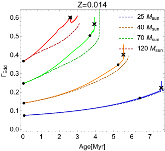
where is the mass loss rate without rotation, is the line-force parameter from CAK theory, is the angular velocity at the stellar surface, and is the Eddington factor
| (4) |
with being the total opacity. Notice that Eq. 3 introduces a correction factor independent of the adopted recipe for mass loss rate without rotation; in other words, can be computed either from Vink’s formula or from Eq. 2. Actually, results from an integration over the surface and the integration accounts for the change of the local mass loss rate with the latitude.
Equation 3 incorporates the impacts on mass loss rate produced not only by rotation but also the radiative acceleration due to the continuum (hence the presence of the Eddington factor), through the so-called -limit. This formulation implies that the stellar break-up or -limit (i.e., when the centrifugal forces compensate gravity in a rotating star) is reached for reduced rotation velocities if is large enough. The velocity associated to this break-up is the so called critical rotational speed,
| (5) |
and hence, the rotation of the star is commonly expressed as a dimensionless ratio between the rotational velocity and this critical value as
| (6) |
On the other hand, the m-CAK prescription incorporates rotational effects in the hydrodynamic solution calculated by HydWind (Curé, 2004), also using as an input. Hydwind solves the equation of motion for the stationary standard line-driven theory,
| (7) |
by finding the eigenfunction that satisfies the velocity profile, , and the eigenvalue, which is proportional to the mass loss rate, (Curé & Rial, 2007). The rotation factor is implicitly included in Eq. 7 by means of , whereas the additional terms are the same as described by Araya et al. (2017, 2021) or Gormaz-Matamala et al. (2022a). In this work, we use moderate to intermediate values of (), therefore all our wind solutions are in the fast wind regime and not in the -slow wind regime which starts approximately from (Araya et al., 2018).
In order to evaluate the effect of the rotation over the self-consistent wind solutions, we repeat the methodology of Paper I and we run evolutionary rotating models in Genec for initial masses of , , , and adopting Vink’s formula for these tracks, hereafter original tracks, as shown in Fig. 1. Then we select a set of representative points over these original tracks, and based on their stellar parameters (, , , ) we calculate the line-force parameters and their respective self-consistent wind parameters and . Initial rotational velocity for all evolution models is , as in Ekström et al. (2012). The results are tabulated in Table 1 where, besides the former columns already included in the Tables 2, 3 and 4 from Paper I, we add the rotation factor as an extra stellar parameter for the input. For each one of the points, we calculate an independent solution for for the tabulated but also for (i.e., without rotation), with their respective self-consistent solution for terminal velocity and mass loss rate. The difference in the self-consistent mass loss due to the incorporation of rotation is expressed as the ratio , which is compared with the correction factor predicted by MM00 (i.e., Eq. 3). Here, we found that both approaches for the rotational effects over produce similar results, which is remarkable considering the error bars associated with the self-consistent mass loss rate. Based on this outcome, we decide to perform our new evolutionary tracks keeping Eq. 3 as correction factor for .
The other physical ingredients related to rotation are the same as in Ekström et al. (2012), Georgy et al. (2013) and Eggenberger et al. (2021). Angular momentum is transported by an advective equation as described in Zahn (1992). The horizontal and vertical shear diffusion coefficients are from respectively Zahn (1992) and Maeder (1997).
3.2 Variation in abundances
Besides the stellar parameters such as temperature, surface gravity, radius and rotation, we included in Table 1 the values for the abundances of helium (expressed as a fraction of the hydrogen abundance by number) and the individual abundances of carbon, nitrogen and oxygen (expressed as a fraction of the solar abundances). Due to the nature of the CNO-cycle, the abundances of helium and nitrogen increase over time, whereas carbon and oxygen decrease (Przybilla et al., 2010). The chemical composition of the surface is enriched in material processed in the core by rotational mixing in the outer radiative envelope. Since we assume that chemical composition in the stellar wind is exactly the same as in the photosphere, the chemical composition of the stellar wind is altered. The question that arises here is, do these alterations in the wind chemical abundances affect the line-acceleration and afterwards the self-consistent mass loss rate?
To solve that question, we artificially alter the individual abundances for the He and the CNO elements from our stellar models of Table 1, and then calculate the respective line-force parameters and self-consistent mass loss rate for each one of the modifications. For example, we compare the for the stellar model P070z10-04 (with N/N) with the expected if N/N, whereas the other individual abundances and the rest of stellar parameters (, , etc.) are kept fixed. Same for the helium: we compare the self-consistent mass loss rate for, e.g., He/H with the expected value for if He/H. These differences are expressed as
| (8) |
with the mass losses tabulated in Table 1, and the self-consistent mass loss rate calculated if the abundance of the evaluated element were solar.
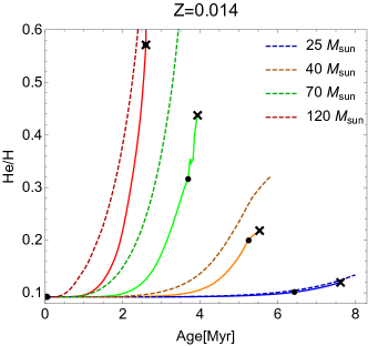
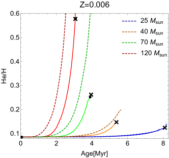
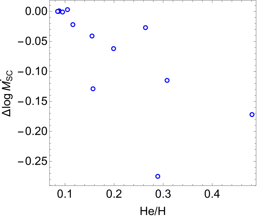
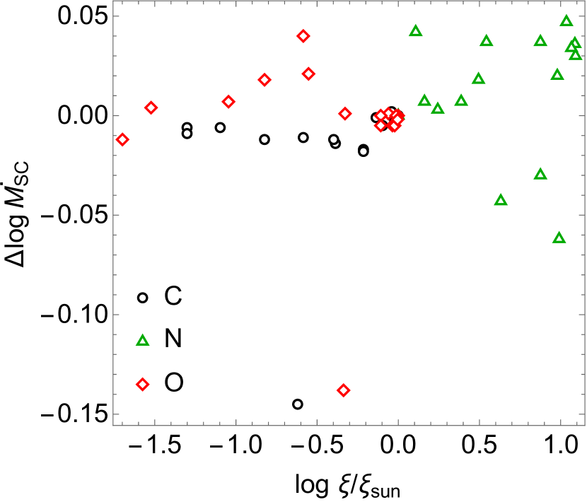
Results of these modifications over the are displayed in Fig. 2(a) for changes in the He/H ratio, and in Fig. 2(b) for modifications of the CNO elements. We see that the variation of each one of the CNO elements even by a factor of barely affects the , keeping the difference close to zero. Indeed, differences in mass loss rate are just of the order of in log scale ( of ), smaller than the error bars shown in Table 1. On the contrary, the increase in the He/H ratio makes decrease in larger magnitudes.
Results from Fig. 2 are quickly explained due to their absolute numbers of the evaluated abundances. Even though the changes in CNO abundances are by a factor of (compared with the initial values at ZAMS), they still represent a small percentage of the total composition of the star. On the contrary, the abundance of helium plays a major role because it grows (in mass fraction) from up to , thus significantly changing the mean molecular weight of the wind. Also, helium abundance is involved in the computation of the ratio and in the radiative acceleration due to Thomson scattering111Here, is the Eddington factor when only free electron scattering opacity is accounted for (the so called classical Eddington factor).
| (9) |
| (10) |
where is the helium abundance by number, is the density of free electrons, and is the proton mass (the meaning of the other symbols are detailed in Curé, 2004, Sec. 2). Hence, when the helium abundance increases, the number of free electrons is reduced and then decreases. As a consequence, the effective mass becomes larger in Eq. 7, and accordingly effective gravity, meaning that the line-acceleration now is able to remove less material as stellar wind (i.e., mass loss rate decreases). However, it is important to mention that this theoretical analysis is made upon the basis of the isolated alteration of the He/H ratio, and therefore this decreasing in the resulting does not imply any modifications in temperature or in any other stellar parameter. For this reason, it differs from the relationship found for Hamann et al. (1995), which was the result of a global analysis over the wind regime of WR stars.
Thus we decide to introduce an extra variable to the recipe of Eq. 2, based on a simple fit of Fig. 2(a)
| (11) |
where (He/H)0 is the He/H ratio at ZAMS (0.085 from Asplund et al., 2009). We see from Table 1 that (He/H)∗ may grow up to at the end of the self-consistent regime, thus leading to a reduction of the mass loss rate of around . However, same as in Paper I, this modification applies only when the self-consistent mass loss rate is adopted in the evolutionary tracks, for kK and , and hence it is still unknown the magnitude of the decreasing factor in prior to the end of the MS, when hydrogen abundance is at the surface.
Finally, details of the formulae used for both old and new evolution models are summarised in Table 2.
| mass loss | End of Main Sequence | |||||||||
|---|---|---|---|---|---|---|---|---|---|---|
| N/C | N/O | |||||||||
| 120.0 | 0.014 | 398.0 | 2.361 | 87.121 | 16.3 | 20.6 | 0.686 | 79.03 | 65.04 | |
| 2.603 | 110.15 | 34.6 | 149.0 | 0.687 | 55.86 | 26.31 | ||||
| 120.0 | 0.006 | 419.0 | 2.513 | 100.504 | 16.5 | 79.7 | 0.694 | 71.32 | 57.79 | |
| 3.070 | 111.196 | 43.4 | 131.0 | 0.694 | 28.94 | 11.14 | ||||
| 70.0 | 0.014 | 360.0 | 4.199 | 42.679 | 18.7 | 7.1 | 0.894 | 73.30 | 69.46 | |
| 3.935 | 60.363 | 26.9 | 3.9 | 0.628 | 18.20 | 5.64 | ||||
| 70.0 | 0.006 | 376.0 | 3.882 | 57.250 | 15.5 | 37.0 | 0.694 | 34.00 | 13.38 | |
| 3.956 | 64.60 | 21.7 | 26.2 | 0.509 | 8.04 | 2.44 | ||||
| 40.0 | 0.014 | 321.0 | 5.794 | 31.86 | 19.2 | 9.9 | 0.553 | 13.86 | 3.90 | |
| 5.535 | 36.428 | 23.6 | 37.4 | 0.460 | 5.46 | 1.50 | ||||
| 40.0 | 0.006 | 334.0 | 5.622 | 36.196 | 16.2 | 30.6 | 0.440 | 6.101 | 1.647 | |
| 5.382 | 38.180 | 18.5 | 71.7 | 0.370 | 3.664 | 0.953 | ||||
| 25.0 | 0.014 | 291.0 | 7.977 | 23.591 | 15.9 | 68.4 | 0.343 | 3.316 | 0.756 | |
| 7.623 | 24.274 | 16.0 | 113.0 | 0.320 | 2.618 | 0.587 | ||||
| 25.0 | 0.006 | 302.0 | 7.708 | 24.272 | 14.1 | 159.0 | 0.309 | 3.389 | 0.687 | |
| 8.105 | 24.567 | 16.7 | 185.0 | 0.331 | 4.267 | 0.786 | ||||
4 Results
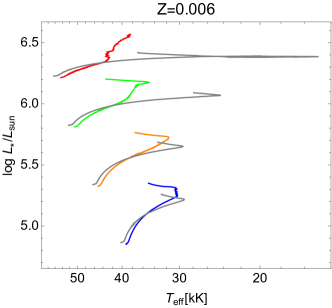
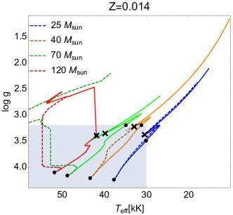
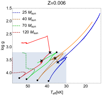
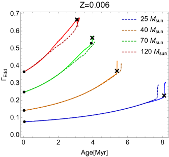
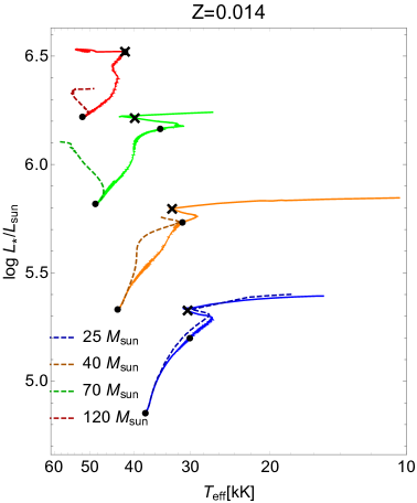
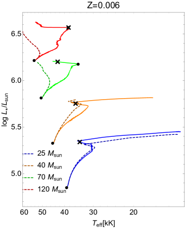
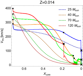
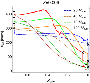
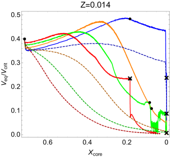
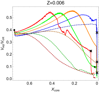
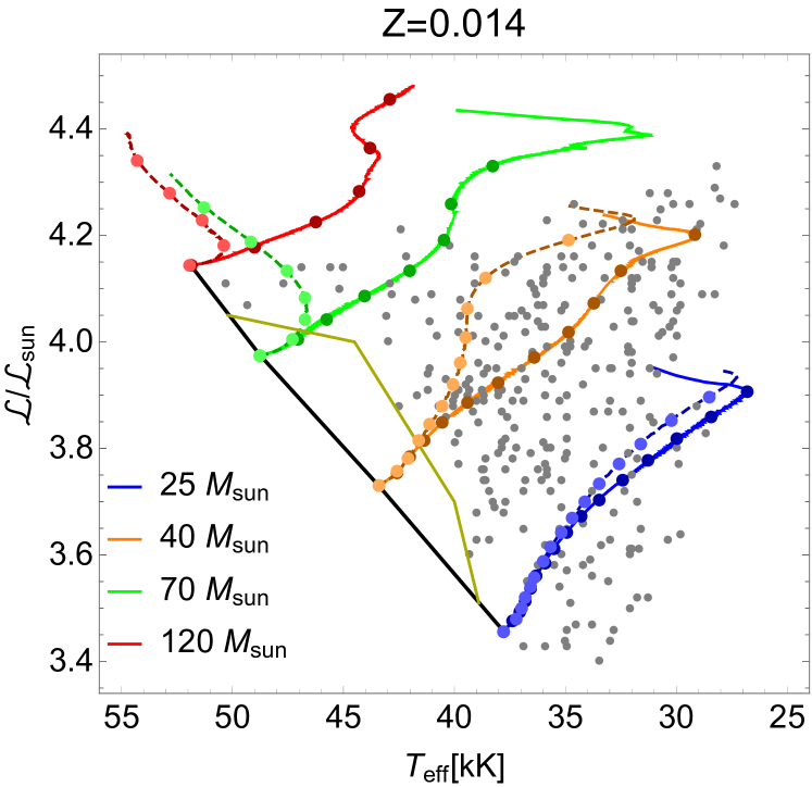
Evolutionary models with rotation, both original and self-consistent, are shown in Fig. 3 in the HR diagram, whereas the rotation and equatorial velocities for tracks adopting both mass loss recipes are shown in Fig. 4. Additional plots such as the comparison with self-consistent non-rotating models from Paper I, the evolutionary tracks in the vs. plane, evolution of the mass loss rate, stellar mass and radii, He/H ratio, Eddington factor, and convective core mass are shown in Appendix A. Also, hereafter all plots comparing new and old recipes of mass loss rate will use solid lines for models with and dashed lines for models with . Major features of the stellar models at the end of the MS, comparing self-consistent tracks with the tracks adopting Vink’s formula (Ekström et al., 2012; Eggenberger et al., 2021), are tabulated in Table 3.
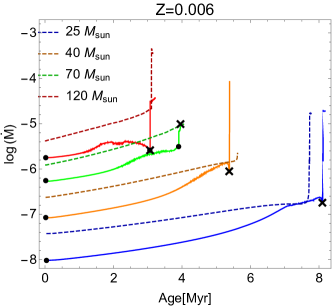
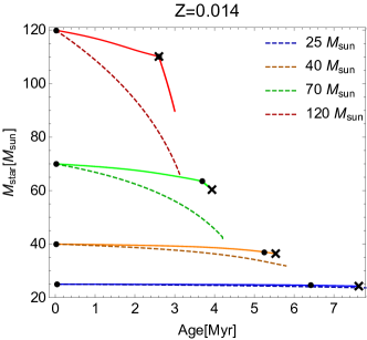
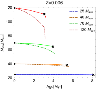
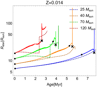
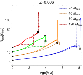
Overall, compared with Paper I (see Table 8 from Gormaz-Matamala et al., 2022b) we find that the lifetime during the main sequence is longer than for the non-rotating models, regardless of the adopted mass loss recipe. The difference with non-rotating models is also appreciated in Fig. 14, where the evolutionary tracks with and without rotation are compared. The rotating tracks remain in bluer regions of the HR diagram compared to the non-rotating ones. Similar to Paper I, self-consistent mass loss rates are of a factor about lower than the mass loss rates from Vink’s formula (Fig. 16), which makes the stars retain more mass (Fig. 17) and have larger radii (Fig. 18) when is adopted. Moreover, besides the straightforward differences in the final masses and the final radii, we also observe that the less strong winds from the self-consistent prescription predict in general weaker surface enrichments of helium and nitrogen at the surface, as seen in the last columns of Table 3 and in the evolution of the He/H ratio (Fig. 19). The only noticeable exception is the model with and , described in detail in the subsection below.
Concerning rotation, self-consistent evolutionary tracks have higher velocities for all models as appreciated in Fig. 4, where we compute equatorial velocities and as a function of the core hydrogen abundance from ZAMS (starting with ) until the end of the main sequence. Same as in Paper I, the largest impact of the new self-consistent mass loss rates are for the higher initial mass stars: the weaker produces stars that rotate faster. Even though the rotational velocity drops down at TAMS for all models, this braking is slower than the one expected for models with the old mass loss recipe. This weaker braking is more prominent for the low metallicity, where the stars adopting keep their rotational velocity almost constant for a longer time before the final deceleration. This implies that, in our regime of metallicities (between and ) mass loss is still a prominent process that impacts the evolution of the rotational velocity. Evolution of rotational velocities is explained by the balance between the transport of angular momentum from the convective core (which is contracting during the main sequence stage) to the stellar surface, and the removal of outer layers due to mass loss (Ekström et al., 2008; de Mink et al., 2013). At extreme low metallicities (), massive stars increase their because their mass losses are not strong enough to counteract the transport of angular momentum from the contracting core (Szécsi et al., 2015). Also for , we see that , which is set initially as , increases up to a constant peak of before the final decrease, as a direct consequence of the initial constancy in the equatorial velocity and the decreasing in the evolution of the critical velocity (Eq. 5). Weaker winds predicts a nearly exponential increasing in the stellar radii for all initial masses and both metallicities (Fig. 18), whereas both the stellar mass and Eddington factor show a linear and metallicity dependent difference with respect to the models computed with the Vink’s formula (Fig. 17 and Fig. 20). Therefore, because they are weaker, self-consistent winds makes our evolution models to approach closer to the break-up limit for rotational velocity in agreement with Ekström et al. (2008), prior to the final drop in at the end of main sequence in agreement with Szécsi et al. (2015).
Now, let us discuss some more detailed effects of the use of the new mass loss rate for the different initial mass models considered in the present work.
4.1 Case
This is the range where we find the very massive stars (VMS Yusof et al., 2013), whose properties and evolution have aroused great interest in recent years (Higgins et al., 2022; Sabhahit et al., 2022). Here, the tracks with have a special relevance because the most studied cluster containing VMSs is 30 Dor, located in the LMC (Crowther et al., 2010; Bestenlehner et al., 2014).
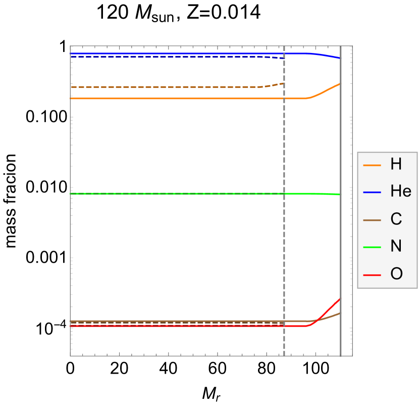
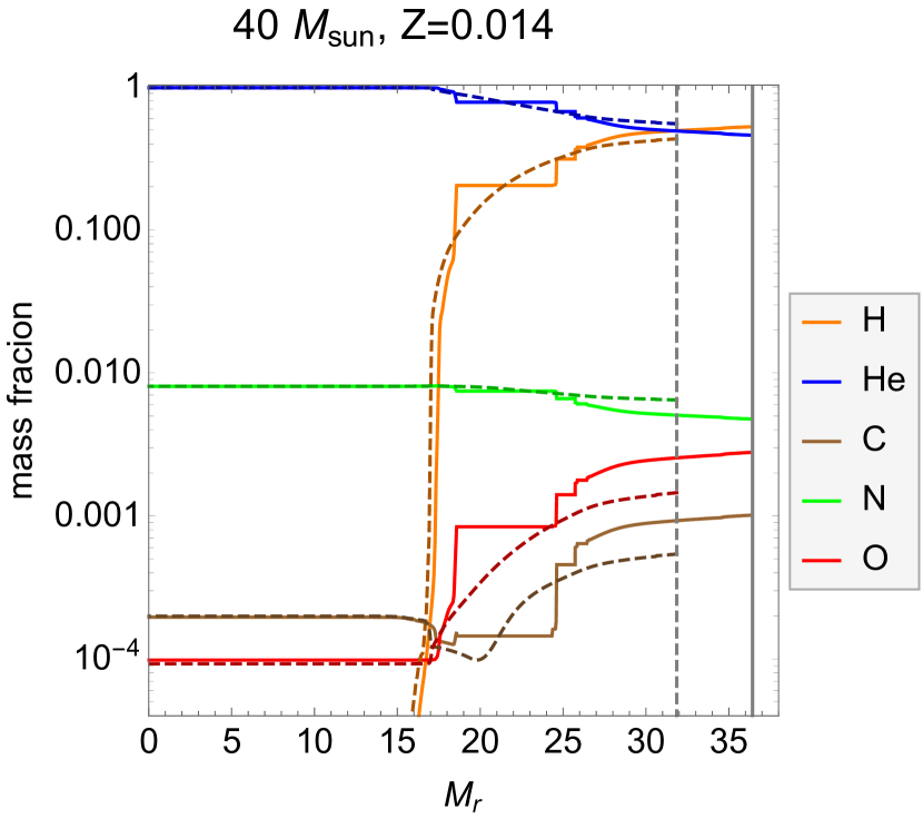
Same as in Yusof et al. (2013), we consider that the star becomes a Wolf-Rayet (i.e., it changes from optically thin to optically thick wind) when its surface hydrogen abundance goes below 0.3 and kK. After that point, mass loss rate is assumed to follow the recipe from Gräfener & Hamann (2008) for WR winds, generating the discontinuity in after the black cross as observed at Fig. 16. Notice that prior to the change in the recipe, evolution of the self-consistent mass loss rate proceeds as expected due to the large increment in the He/H ratio (Fig. 19) as a consequence of Eq. 11. Due to the extreme strength of the winds, the VMS is depleted from the of its surface hydrogen even before H is completely exhausted in its core, as seen from Fig. 6(a), generating the stars with spectral type WNh (Hamann et al., 2006; Martins & Palacios, 2022). This switch not only in the prescription but also in the wind regime (from optically thin to optically thick wind) is also evidenced by Fig. 18, where the radius needs to the recalculated after the black crosses based on the wind opacity (see, e.g, Meynet & Maeder, 2005) due to the absence of a well-defined photosphere (Schaller et al., 1992).
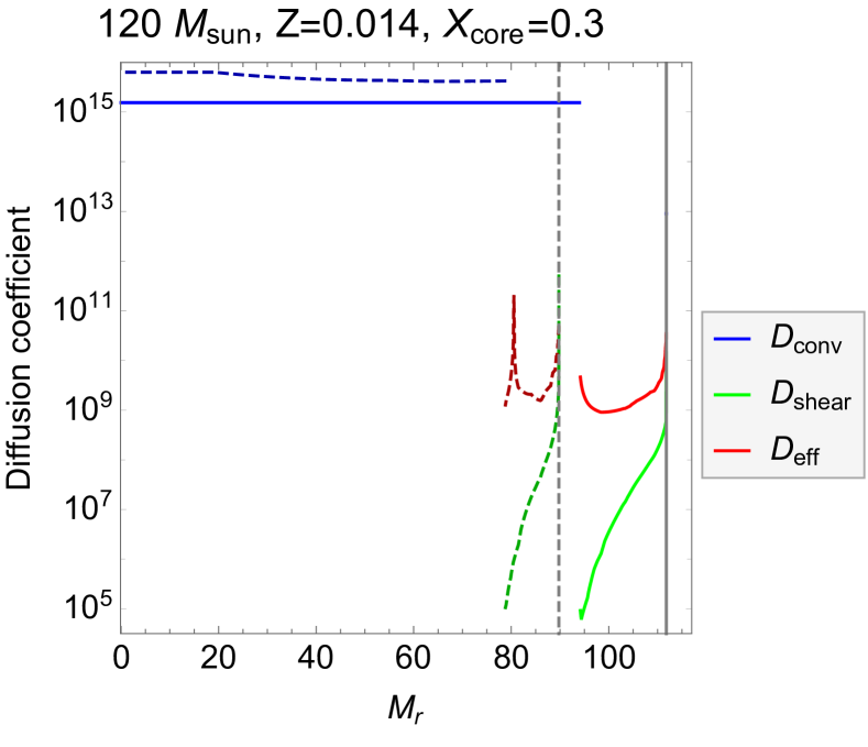
The most remarkable difference between classical and self-consistent tracks in Fig. 3, is the drift ‘redwards’ (i.e., towards the cool range of temperatures in the HRD) that the self-consistent models do since the beginning of the main sequence. For both metallicities, stars with end their MS lifetime as O-type at kK, before suddenly increasing their temperature and becoming WNh stars. We note that the model using the weaker self-consistent shows in general a slightly stronger surface enrichment than the original model. This explains why these models evolve to redder regions of the HRD during the MS phase. It is a well known effect that a star showing a nearly homogeneous internal chemical composition keep blue colours in the HRD diagram (Maeder, 1987). A homogeneous chemical composition can result from a very strong internal mixing, from very strong mass losses or from both processes. In contrast an internal non-homogeneous composition will produce redwards evolution on the HRD. The extension to the red is favoured when a larger convective core is present and the radiative envelope is not too efficiently mixed, otherwise we would have a situation approaching the one of a homogeneous internal composition and the track will remain in the blue region of the HRD (Martinet et al., 2021). Here we see that reducing the mass loss favours redwards tracks. In Fig. 5, we show the diffusion coefficients in the new and old mass loss rate models in the middle of the MS phase. For the case of and , the model with a lower mass loss rate has a more massive convective core at that stage, even though it represents a slightly minor fraction of the total mass: for the self-consistent model, against for the old one. This is a result of the higher difference in the mass retained and also to the possible higher value of the effective diffusion coefficient, , just above the convective core. In the rest of the radiative envelope, there is not much difference between the values of . Since the diffusion timescale varies as , and since the radius of the self-consistent model is larger, we see that the self-consistent model will take a longer time to reach a given level of surface enrichment than the original one. This imposes redder evolutionary tracks for the model with .
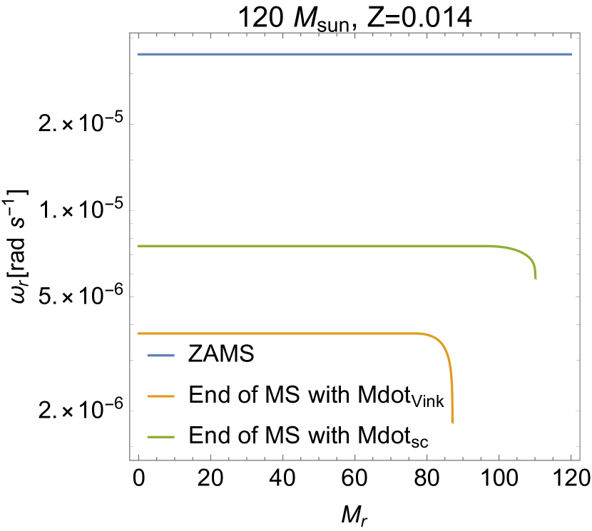
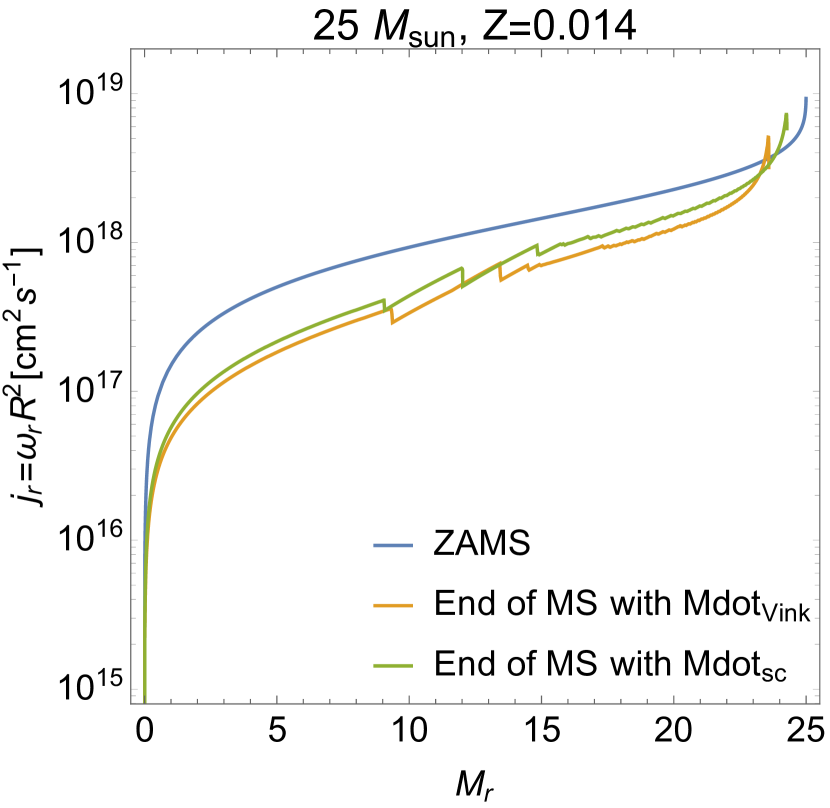
Figure 6(a) compares the chemical composition of the self-consistent and original models at the end of the MS phase. As expected the model with the lower mass loss rate is showing the greatest contrasts between the surface composition and that of the core. Figure 7(a) shows the variation of the specific angular momentum inside the at the beginning and end of the MS phase for the two different mass loss prescriptions. Let us first remind that in the absence of any angular momentum transport, remains constant. The evolution that we see between the beginning and end of the core H-burning phase (a global decrease of in the whole star) is due to the fact that the transport processes will in general transport angular momentum from the inner to the outer layers of the star. At the surface the angular momentum is removed by stellar winds, thus we see that when the mass loss rates are smaller, is larger. Indeed, by decreasing the mass loss rate by about a factor three during the main sequence (compared to Vink’s formula), we obtain that the specific angular momentum is shifted by dex upwards when is used, whereas the value of the angular velocity of the core is increased by a factor of (see Fig. 7(b)).
Finally, we notice that for both metallicities our rotating models reach the WNh stage at kK. Since we know that stars will increase their temperature through the WR stage, this means that rotating models with do not cross the temperature regime around kK during their MS phase, where the so-called bi-stability jump (Vink et al., 1999) takes place. Because of this reason, and contrary to the non-rotating models from Paper I, we do not observe LBV behaviour such as eruptive mass losses at this mass range. The fact that only initially slow rotating models can go through an eruptive mass loss regime at the end of the main sequence supports the idea that the LBV phenomenon is very rare for very massive stars (Gräfener, 2021).

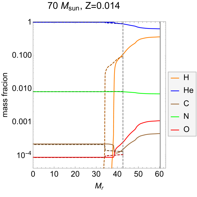
4.2 Case
Same as before, besides the differences in the stellar mass (Fig. 17) we also observe a divergence bluewards-redwards for the evolution across the HR diagram (Fig. 3). However, unlike the previous case, this time the beginning of the WR winds stage coincides with the end of the H-core burning, which can be appreciated in Fig. 6(b) where hydrogen is depleted in the core at the end of both (standard and self-consistent) tracks. Again we see the change in the slope of the evolution in mass loss rate (Fig. 16), this time with a flattening in prior to reaching the second black dot, associated with the increasing of the He/H ratio (Fig. 19).
Concerning rotation, the braking in the equatorial velocity only becomes significant after the star has burnt almost half of the hydrogen in its core: for and for , which also represents the peak of for Galactic metallicities and for SMC metallicities (Fig. 4). This is interconnected one more time with the retaining of more specific angular momentum for the models adopting , and with the larger stellar radii (Fig. 18). Indeed, the switch in the wind regime from to (marked with an abrupt increase in mass loss rate after the second black dot of Fig. 16) carries an important drop in the rotational velocity which creates some numerical instability, but does not affect the general trend in the evolution of observed for all the rotation models.
From Fig. 6(b), we see that the variation of the element abundances across the stellar structure from core to surface is more prominent for the model with , which is evidence for the less efficient rotational mixing for the weaker wind. However, on the contrary of the case with , where the inner structure was almost fully homogeneous, now there are remarkable distinctions between core and surface abundances because the mass loss has been less efficient in reducing the mass of the envelope and revealing the inner layers.
The redward drift of the evolutionary tracks for the reduced mass loss rate models is in line with the results found by Björklund et al. (2022), who implemented a mass loss recipe derived from the wind theoretical prescription from Björklund et al. (2021) where is also times below the values coming from Vink’s formula. In their study, they used Mesa to trace the evolutionary track of a star with , km s-1, and solar metallicity; where they found the drift bluewards at kK (see their Fig. 6). On our side, by making an eye inspection on Fig. 3 and Fig. 14, we conjecture that the point of turning bluewards for one of our self-consistent models with and must be between kK, i.e., around kK hotter than found by Björklund et al. (2022). Such a discrepancy is relatively minor considering the differences between Genec and Mesa (check the comparison for the models of these both codes, as done by Agrawal et al., 2022). Therefore, we can conclude that the self-consistent m-CAK prescription for stellar winds predicts evolutionary tracks in fair agreement with the recent study of Björklund et al. (2022), as expected given that both studies are based on mass loss rates of the same order of magnitude.
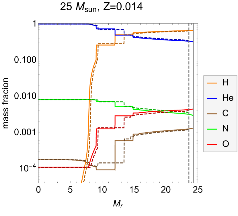
4.3 Cases and
Effects of self-consistent mass loss rates over the evolution of stars within these mass ranges are less pronounced, as it is seen in Fig. 3 and in the resulting final masses and radii from Table 3. We also observe a ‘redder’ evolution for the models adopting , but still ‘bluer’ compared with non rotating cases (Fig. 14). Differences in the rotational velocities are also less remarkable, though they still follow the same trend of the more massive models. For the case of (LMC), we observe that the end of H-burning is reached inside the region of validity of the self-consistent tracks (Fig. 15), and therefore the second dot overlaps again with the cross. Because we observe this situation only with (SMC) in the non-rotating cases from the Paper I, it implies that the evolution models adopting m-CAK wind prescription cover a broader range of the main sequence when rotation is incorporated.
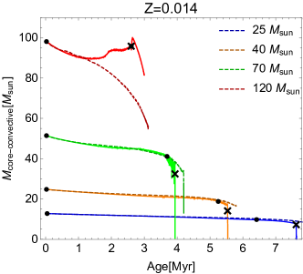
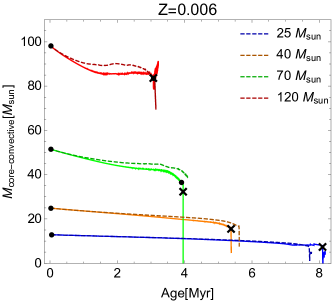
The impact of the different mass losses on the chemical structures of the and stellar models can be seen in Fig 8. The convective cores are and for the and stars, respectively, when the high mass loss rates are used (Fig. 21). The composition in the radiative envelope shows some significant differences between the two models. This is particularly visible for the star, where in the low mass loss rate model a convective region is associated to the H-burning shell (between about and coordinates), while no convective zone is associated to that shell in the high mass loss rate model. We see therefore, that reducing the mass of the envelope disfavours the formation of an intermediate convective shell associated to the H-burning shell.
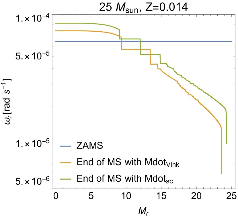
The specific angular momentum inside our model of is shown in Fig. 9(a). We see along the curves small abrupt variations (as for instance around at the end of the MS phase). These come from regions where there is a transition between a convective and a radiative zone, where the chemical composition changes, also observed as an abrupt jump in the inner angular velocity (Fig. 9(b)). Like for the star, the model computed with the self-consistent mass loss rates ends the MS phase with slightly larger values of the specific angular momentum. The increase is less strong since the mass loss rates are anyway weaker when the initial mass decreases. The changes in the interior angular velocity distribution are also much weaker than for the model. We note as expected a slightly faster rotating core in the self-consistent stellar model compared to the original one.
5 Comparison with rotational surveys
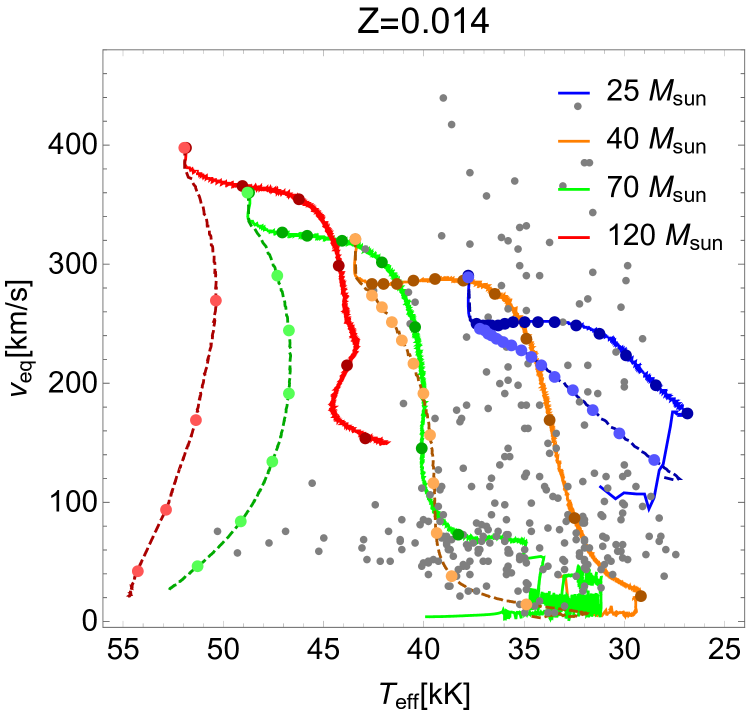
Because the self-consistent m-CAK prescription predicts less strong winds than previous studies, stellar models computed with such prescription evolve at higher luminosities and reach larger radii during the MS phase than the models of Ekström et al. (2012) or Eggenberger et al. (2021), as already detailed in Section 4. Besides, evolutionary tracks adopting also predict that the rotational velocity during the main sequence will be higher as seen in Fig. 4, implying a weaker braking in the equatorial velocity of massive stars. This weaker braking is also represented in Fig. 10, where we plot rotational velocities as a function of the effective temperatures for evolutionary tracks adopting old and new winds, and where the timesteps of Myr are illustrated with the respective coloured circles. Velocities from evolution models with quickly decreases after the first Myr, passing from little variations in temperature for to moderate variations for . On the contrary, the from self-consistent evolutionary tracks keep relatively constant at the beginning of the main sequence for all tracks, at timescales inversely proportional to their initial masses (from Myr for to Myr for ), whereas decreases kK per each model prior to the final braking.
In parallel, we plot in Fig. 10 the sample of 285 O-type stars taken from the recent survey of Holgado et al. (2022), whose catalog is available online222https://cdsarc.cds.unistra.fr/viz-bin/cat/J/A+A/665/A150. In their study, they revisited the rotational properties of 285 Galactic massive O-type as part of the IACOB Project (Simón-Díaz et al., 2015; Holgado et al., 2018, 2020). This survey covers a range of stellar masses from to solar masses, and a mixture of ages within the main sequence stage. Besides, they compared the rotation of these stars with the state-of-the-art evolution models Brott et al. (2011) and Ekström et al. (2012), finding that neither of the two sets of rotating evolutionary tracks was able to reproduce such features of the survey. From one side, models from Brott et al. (2011) cannot reproduce the existence of stars with km s-1 across the entire domain of O-type stars (see Fig. 9 of Holgado et al., 2022). From the other side, models from Ekström et al. (2012) cannot adequately reproduce the scarcity of stars with km s-1 for the left side of Fig. 10, which is also appreciated by the lack of stars matching the old tracks with and .
In contrast, in Fig. 10 we observe that new self-consistent evolutionary tracks can adequately explain both issues. Tracks from to match to the set of stars with rotational velocities below 150 km s-1 for the range of temperatures from to kK. Also, the empty region of stars with kK and km s-1 would only be populated by our model, which is out of the mass range of the sample. Therefore, evolution models adopting weaker winds better interpret the rotational properties of the survey of Holgado et al. (2022), keeping with initial and without the need of decreasing the initial equatorial velocity for our models.
Nonetheless, despite this encouraging result, there are still important aspects of the rotational properties of Galactic O-type stars that need to be taken into account. For instance, although our track of can encircle a larger fraction of stars in the top-right side of Fig. 10, there are still fast rotators ( km s-1) outside the scope of any track, which only could be explained by binary interaction effects (de Mink et al., 2013; Wang et al., 2020). Moreover, the slow braking observed for self-consistent evolutionary tracks indicates that stars born with masses between and should spend the of the lifetime in the main sequence stage with between km s-1 and km s-1. As a consequence, we should expect to find a larger fraction of O-type stars in this range of rotational velocities. However, because of its proximity to the ZAMS, this range also covers an important portion of the region where there is a lack of empirically detected O-type stars, as shown in the Fig. 11 and described by Holgado et al. (2020). For that reason, it is not surprising to find a moderate number of stars in the range from to km s-1 and temperatures between and kK. Therefore, even though our evolution models adopting self-consistent winds represent a relevant upgrade, there are still important challenges in the study of O-type stars to deal with, such as the expansion of current samples to more hidden places by the use of infrared observations.
6 Implications of evolution models with self-consistent winds
The evolutionary tracks across the HRD from our rotating models adopting self-consistent winds exhibit considerable contrasts with the old models adopting Vink’s formula, leading into a better description of the rotational properties of the most recent observational diagnostics. In this Section we move one step beyond, and we explore some of the implications that the incorporation of these self-consistent models have at Galactic scale. We remark however that these implications are here discussed at an introductory level, and their respective conclusions are part of forthcoming studies.
6.1 Enrichment of the 26Al isotope
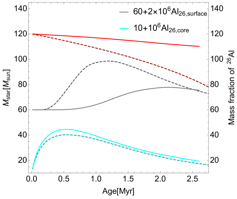
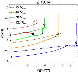
Figure 12 shows how the new mass loss rates impact the quantity of 26Al ejected by the stellar winds of our models computed with the two mass loss rate prescriptions. Compared to the models discussed in Paper I for the non rotating case, the current rotating models allow 26Al to appear at the surface well before layers enriched by nuclear burning in 26Al are uncovered by the stellar winds. This is the effect of the rotational mixing that allows diffusion of the 26Al produced in the core to reach the surface. Thus we see that, like for the case in Paper I, reducing the mass loss rate reduces the maximum value of the abundance of 26Al reached at the surface. This maximum also occurs at a more advanced age for the model with self-consistent wind, despite the peak of production of 26Al in the core is found at almost the same age for both (old and new) wind prescriptions. Such time difference between the peak abundance at the centre and at the surface is easily explained by the reduction on mass loss rate, which makes the star to take more time to remove their outer layers and then expose its inner composition, and for the less intense mixing as previously evidenced in Fig. 6(a).
| Track | ||
|---|---|---|
| non-rotating | rotating | |
| Classic | ||
| Self-consistent | ||
The total amount of 26Al released from the stellar surface to the interstellar medium during the MS for each one of our wind prescriptions, together with previous results from Paper I, are tabulated in Table 4. Although the total amount of the aluminium-26 ejected by old winds is almost the same regardless if rotation is considered, for self-consistent winds the rotating model predicts the ejection of times less fraction of the isotope during the MS, compared to the rotating evolution model adopting Vink’s formula. Such a difference is related not only to the mass loss due to the line-driven mechanism. Whereas non-rotating models predict eruptive processes associated to LBVs (Fig. 7 from Paper I), rotating models for never reach those magnitudes for (Fig. 16). Therefore, the contribution of 26Al to the interstellar medium predicted by self-consistent winds is even weaker (compared with models adopting Vink’s formula) for rotating models than for non-rotating models.
However, it is important to remark that Fig. 12 covers only the lifetime of the star when the wind is optically thick, then excluding optically thick winds from WNh (H-core burning) and WR (He-core burning) phases. In contrast, the study of Martinet et al. (2022) calculated the evolution of 26Al for evolution models with mass ranges from to and metallicities from to , but without making any distinction between thin and thick wind regimes. Instead, they made the distinction between H-core and He-core burning stages, showing that the production of 26Al abruptly decreases when the star enters into the He-burning. As a consequence, even though here we are selecting only one mass and one metallicity to do a quick comparison with the more complete analysis from Martinet et al. (2022), we infer that the larger contribution of 26Al from very massive stars to the ISM must stem from the later stages exhibiting optically thick winds, such as H-core WNh stars, to explain the current estimations of 26Al total abundance in the Milky Way (Knödlseder, 1999; Diehl et al., 2006; Wang et al., 2009; Pleintinger et al., 2019). Certainly, we need a extensive study implementing self-consistent evolution models for wider ranges of masses and metallicities, together with updates in the convection criteria (Georgy et al., 2014; Kaiser et al., 2020) and overshooting values (Martinet et al., 2021) in order to have more complete analysis.
6.2 Massive stars at the Galactic Centre
The implications of the new evolution models for massive stars with self-consistent mass loss rate are large, not only across the main sequence but also over the subsequent evolutionary stages. One of such consequences is how using models computed with the weaker self-consistent mass loss rates may actually provide estimates of evolutionary masses that are lower than when models with from Vink et al. (2001) are adopted.
An example of this situation is the study of the Ofpe333Ofpe is a spectral classification for stars showing intermediate properties between O-type and WR stars (Walborn, 1977, 1982). For that reason, they are assumed to be a transition between both spectroscopic phases according to the Conti scenario (Conti, 1975). stars located at the Galactic Centre. Massive stars at the Galactic Centre play an important role feeding the supermassive black hole Sgr A* by means of their stellar winds (Cuadra et al., 2015; Ressler et al., 2018; Calderón et al., 2020b). This is a consequence of the remarkable situation of OB and WR stars representing a large fraction of the stars at the Galactic Centre (e.g., Lu et al., 2013; von Fellenberg et al., 2022), even though this is a region thought to be hostile to star formation (e.g., Genzel et al., 2010). The wind properties of these massive stars have been analysed and constrained by Martins et al. (2007) for the O-type and WRs, and by Habibi et al. (2017) for the B-type stars. Martins et al. (2007) calculated the stellar and wind parameters for a set of stars at evolved stages such as Ofpe and WN, which are particularly relevant for feeding Sgr A*. Their analysis was performed by spectral fitting using the CMFGEN code and the evolutionary tracks from Meynet & Maeder (2005). Therefore, it is important to check whether the state-of-the-art evolutionary tracks suggest a revision of the properties of the massive stars at the Galactic Centre, and the consequences these modifications imply for the accretion on to Sgr A*.
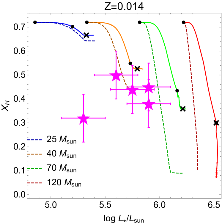
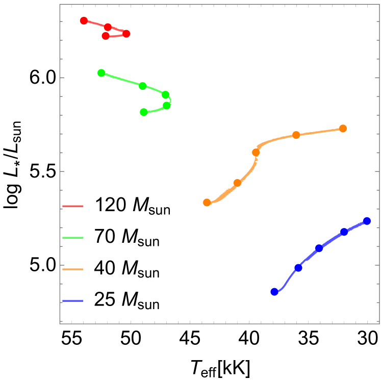
To illustrate the issue, Fig. 13 shows the hydrogen abundance at the stellar surface as a function of luminosity for standard and self-consistent evolutionary tracks, plus five of the Ofpe stars analysed by Martins et al. (2007, compare with their Fig. 21). From Fig. 13 we can see that for a given hydrogen surface abundance and for a given initial mass, the tracks computed with the weaker self-consistent mass-loss rates are overluminous. These tracks also end the MS phase with higher surface hydrogen abundances. We notice that the lowest luminosity Ofpe star in the sample cannot be reproduced by any of the two families of tracks. The other four stars can reasonably be fitted by both types of models. On average, although the initial masses that will be deduced from comparison with self-consistent mass-loss rate tracks are smaller than the masses deduced from tracks computed with Vink’s mass loss rates.
Given that the observed Ofpe stars in the Galactic center would have lower initial masses, we can speculate that their wind parameters (terminal velocity and mass loss rate) will be lower as well. The terminal velocity is an important parameter in this context, since the Galactic centre is a region with large stellar density, and the winds collide with each other, creating a high-temperature medium. However, slower winds ( km/s) produce a plasma of lower temperature ( K) at the collision, which becomes susceptible to hydrodynamical instabilities and ends up forming high-density clumps and streams. These clumps can then be captured by the central black hole, increasing its accretion rate (Cuadra et al., 2005, 2008; Calderón et al., 2016, 2020b, 2020a).
In a forthcoming paper we will perform a more complete analysis of the Galactic Centre massive star population, extending the tracks to the WR stage and taking into account the non-standard chemical abundance deduced for this region. From the observational side, we will also include data collected after Martins et al. (2007), which is expected to afford a reduction in the typical error bars for the stellar luminosities from down to dex (S. von Fellenberg, priv. comm.). The comparison between models and observations will allow us to update the estimates for the initial masses and ages of this population, and also its wind parameters, which have a large influence on the current accretion on to Sgr A*.
7 Conclusion
We have extended the stellar evolution models performed in Gormaz-Matamala et al. (2022b, Paper I), adopting self-consistent m-CAK prescription (Gormaz-Matamala et al., 2019, 2022a) for the mass loss rate recipe (Eq. 2), by including the rotational effects. Stellar rotation affects the mass loss of a massive star, not only by changing the balance between gravitational, radiative and centrifugal forces (Maeder & Meynet, 2000), but also because rotational mixing considerably modifies the internal distribution of the chemical elements and thus impacts the evolutionary tracks in the HRD and hence the mass loss rates. The progressive increase of the helium-to-hydrogen ratio in the wind impacts the line-force parameters and henceforth the self-consistent solution of the equation of motion, leading to a decrease of 0.2 dex in the absolute value of the mass loss rate (Eq. 11).
The updated mass loss rates are implemented for a set of evolutionary models at different initial stellar masses, for metallicities (Galactic) and (LMC). New tracks show important differences with respect to the studies of Ekström et al. (2012) and Eggenberger et al. (2021), who adopted the formula from Vink et al. (2001) for the winds of massive stars, but exhibit a fair proximity with the studies of Sabhahit et al. (2022) for VMS, and with Björklund et al. (2022) and their own self-consistent wind prescription. Besides the differences in the tracks across the HRD, already remarked in Paper I, for rotating evolutionary tracks we find as expected that the surface rotation maintains a higher value when the weaker self-consistent mass loss rates are adopted. We observe that for the initial rotation considered here, tracks computed with the self consistent mass loss rates extend more to the red part of the HR diagram during the MS phase Such an effect is more important for masses above about .
New tracks predict evolution of the surface rotational velocities for O-type stars that, at first sight, appear to be in better agreement with the most recent observational diagnostics. The slow braking in the evolution of explains better the rotational properties of the survey of Holgado et al. (2022) for O-type stars, such as the lack of fast rotators for stars with kK and the abundance of stars with km s-1 and temperatures between 27 and 40 kK. Besides, the implications of these new evolution models are wide. For example, lower mass loss rate predicts a less important stellar wind contribution to the Aluminium-26 enrichment of the ISM during the main sequence phase, at least whereas the stellar wind is optically thin. Likewise, the fact that self-consistent models are more luminous in the HRD suggests that the initial mass deduced from evolutionary tracks might be lower when the self-consistent tracks are used. This may apply to the mass estimates of Ofpe and WN stars at the Galactic Centre, which leads us to expect that their wind properties (mass loss rate and terminal velocity) might also be overestimated. Nevertheless, a more accurate analysis of the stars surrounding Sgr A* and their stellar winds are deferred to a forthcoming paper.
Acknowledgements.
We are very grateful for the anonymous referee and their very constructive comments and feedback. We also acknowledge useful discussions with Sebastiano von Fellenberg and Stefan Gillessen. This project was partially funded by the Max Planck Society through a “Partner Group” grant. JC acknowledges financial support from FONDECYT Regular 1211429. GM has received funding from the European Research Council (ERC) under the European Union’s Horizon 2020 research and innovation programme (grant agreement Nº 833925, project STAREX). MC thanks the support from FONDECYT projects 1190485 and 1230131.References
- Abbott et al. (2016) Abbott, B. P., Abbott, R., Abbott, T. D., et al. 2016, ApJ, 818, L22
- Abbott (1982) Abbott, D. C. 1982, ApJ, 259, 282
- Agrawal et al. (2022) Agrawal, P., Szécsi, D., Stevenson, S., Eldridge, J. J., & Hurley, J. 2022, MNRAS, 512, 5717
- Araya et al. (2021) Araya, I., Christen, A., Curé, M., et al. 2021, MNRAS, 504, 2550
- Araya et al. (2018) Araya, I., Curé, M., ud-Doula, A., Santillán, A., & Cidale, L. 2018, MNRAS, 477, 755
- Araya et al. (2017) Araya, I., Jones, C. E., Curé, M., et al. 2017, ApJ, 846, 2
- Asplund et al. (2005) Asplund, M., Grevesse, N., & Sauval, A. J. 2005, in Astronomical Society of the Pacific Conference Series, Vol. 336, Cosmic Abundances as Records of Stellar Evolution and Nucleosynthesis, ed. I. Barnes, Thomas G. & F. N. Bash, 25
- Asplund et al. (2009) Asplund, M., Grevesse, N., Sauval, A. J., & Scott, P. 2009, ARA&A, 47, 481
- Belczynski et al. (2010) Belczynski, K., Bulik, T., Fryer, C. L., et al. 2010, ApJ, 714, 1217
- Bestenlehner et al. (2014) Bestenlehner, J. M., Gräfener, G., Vink, J. S., et al. 2014, A&A, 570, A38
- Björklund et al. (2021) Björklund, R., Sundqvist, J. O., Puls, J., & Najarro, F. 2021, A&A, 648, A36
- Björklund et al. (2022) Björklund, R., Sundqvist, J. O., Singh, S. M., Puls, J., & Najarro, F. 2022, arXiv e-prints, arXiv:2203.08218
- Bouret et al. (2012) Bouret, J. C., Hillier, D. J., Lanz, T., & Fullerton, A. W. 2012, A&A, 544, A67
- Brott et al. (2011) Brott, I., de Mink, S. E., Cantiello, M., et al. 2011, A&A, 530, A115
- Calderón et al. (2016) Calderón, D., Ballone, A., Cuadra, J., et al. 2016, MNRAS, 455, 4388
- Calderón et al. (2020a) Calderón, D., Cuadra, J., Schartmann, M., et al. 2020a, MNRAS, 493, 447
- Calderón et al. (2020b) Calderón, D., Cuadra, J., Schartmann, M., Burkert, A., & Russell, C. M. P. 2020b, ApJ, 888, L2
- Castor et al. (1975) Castor, J. I., Abbott, D. C., & Klein, R. I. 1975, ApJ, 195, 157
- Conti (1975) Conti, P. S. 1975, Memoires of the Societe Royale des Sciences de Liege, 9, 193
- Crowther et al. (2010) Crowther, P. A., Schnurr, O., Hirschi, R., et al. 2010, MNRAS, 408, 731
- Cuadra et al. (2008) Cuadra, J., Nayakshin, S., & Martins, F. 2008, MNRAS, 383, 458
- Cuadra et al. (2005) Cuadra, J., Nayakshin, S., Springel, V., & Di Matteo, T. 2005, MNRAS, 360, L55
- Cuadra et al. (2015) Cuadra, J., Nayakshin, S., & Wang, Q. D. 2015, MNRAS, 450, 277
- Curé (2004) Curé, M. 2004, ApJ, 614, 929
- Curé & Rial (2007) Curé, M. & Rial, D. F. 2007, Astronomische Nachrichten, 328, 513
- de Mink et al. (2013) de Mink, S. E., Langer, N., Izzard, R. G., Sana, H., & de Koter, A. 2013, ApJ, 764, 166
- Diehl et al. (2006) Diehl, R., Halloin, H., Kretschmer, K., et al. 2006, Nature, 439, 45
- Eggenberger et al. (2021) Eggenberger, P., Ekström, S., Georgy, C., et al. 2021, A&A, 652, A137
- Eggenberger et al. (2008) Eggenberger, P., Meynet, G., Maeder, A., et al. 2008, Ap&SS, 316, 43
- Ekström et al. (2012) Ekström, S., Georgy, C., Eggenberger, P., et al. 2012, A&A, 537, A146
- Ekström et al. (2008) Ekström, S., Meynet, G., Maeder, A., & Barblan, F. 2008, A&A, 478, 467
- Event Horizon Telescope Collaboration et al. (2022) Event Horizon Telescope Collaboration, Akiyama, K., Alberdi, A., et al. 2022, ApJ, 930, L16
- Genzel et al. (2010) Genzel, R., Eisenhauer, F., & Gillessen, S. 2010, Reviews of Modern Physics, 82, 3121
- Georgy et al. (2013) Georgy, C., Ekström, S., Eggenberger, P., et al. 2013, A&A, 558, A103
- Georgy et al. (2011) Georgy, C., Meynet, G., & Maeder, A. 2011, A&A, 527, A52
- Georgy et al. (2014) Georgy, C., Saio, H., & Meynet, G. 2014, MNRAS, 439, L6
- Gormaz-Matamala et al. (2019) Gormaz-Matamala, A. C., Curé, M., Cidale, L. S., & Venero, R. O. J. 2019, ApJ, 873, 131
- Gormaz-Matamala et al. (2021) Gormaz-Matamala, A. C., Curé, M., Hillier, D. J., et al. 2021, ApJ, 920, 64
- Gormaz-Matamala et al. (2022a) Gormaz-Matamala, A. C., Curé, M., Lobel, A., et al. 2022a, A&A, 661, A51
- Gormaz-Matamala et al. (2022b) Gormaz-Matamala, A. C., Curé, M., Meynet, G., et al. 2022b, A&A, 665, A133
- Gräfener (2021) Gräfener, G. 2021, A&A, 647, A13
- Gräfener & Hamann (2008) Gräfener, G. & Hamann, W. R. 2008, A&A, 482, 945
- Groh et al. (2014) Groh, J. H., Meynet, G., Ekström, S., & Georgy, C. 2014, A&A, 564, A30
- Habibi et al. (2017) Habibi, M., Gillessen, S., Martins, F., et al. 2017, ApJ, 847, 120
- Hamann et al. (2006) Hamann, W. R., Gräfener, G., & Liermann, A. 2006, A&A, 457, 1015
- Hamann et al. (1995) Hamann, W. R., Koesterke, L., & Wessolowski, U. 1995, A&A, 299, 151
- Heger et al. (2003) Heger, A., Fryer, C. L., Woosley, S. E., Langer, N., & Hartmann, D. H. 2003, ApJ, 591, 288
- Higgins et al. (2022) Higgins, E. R., Vink, J. S., Sabhahit, G. N., & Sander, A. A. C. 2022, MNRAS, 516, 4052
- Holgado et al. (2018) Holgado, G., Simón-Díaz, S., Barbá, R. H., et al. 2018, A&A, 613, A65
- Holgado et al. (2020) Holgado, G., Simón-Díaz, S., Haemmerlé, L., et al. 2020, A&A, 638, A157
- Holgado et al. (2022) Holgado, G., Simón-Díaz, S., Herrero, A., & Barbá, R. H. 2022, A&A, 665, A150
- Iglesias & Rogers (1996) Iglesias, C. A. & Rogers, F. J. 1996, ApJ, 464, 943
- Kaiser et al. (2020) Kaiser, E. A., Hirschi, R., Arnett, W. D., et al. 2020, MNRAS, 496, 1967
- Keszthelyi et al. (2017) Keszthelyi, Z., Puls, J., & Wade, G. A. 2017, A&A, 598, A4
- Knödlseder (1999) Knödlseder, J. 1999, ApJ, 510, 915
- Krtička & Kubát (2017) Krtička, J. & Kubát, J. 2017, A&A, 606, A31
- Krtička & Kubát (2018) Krtička, J. & Kubát, J. 2018, A&A, 612, A20
- Langer & Kudritzki (2014) Langer, N. & Kudritzki, R. P. 2014, A&A, 564, A52
- Lattimer & Cranmer (2021) Lattimer, A. S. & Cranmer, S. R. 2021, ApJ, 910, 48
- Lu et al. (2013) Lu, J. R., Do, T., Ghez, A. M., et al. 2013, ApJ, 764, 155
- Maeder (1987) Maeder, A. 1987, A&A, 178, 159
- Maeder (1997) Maeder, A. 1997, A&A, 321, 134
- Maeder & Meynet (2000) Maeder, A. & Meynet, G. 2000, A&A, 361, 159
- Maeder & Meynet (2010) Maeder, A. & Meynet, G. 2010, New A Rev., 54, 32
- Martinet et al. (2021) Martinet, S., Meynet, G., Ekström, S., et al. 2021, A&A, 648, A126
- Martinet et al. (2022) Martinet, S., Meynet, G., Nandal, D., et al. 2022, A&A, 664, A181
- Martins et al. (2007) Martins, F., Genzel, R., Hillier, D. J., et al. 2007, A&A, 468, 233
- Martins & Palacios (2022) Martins, F. & Palacios, A. 2022, A&A, 659, A163
- Meynet & Maeder (2005) Meynet, G. & Maeder, A. 2005, A&A, 429, 581
- Noebauer & Sim (2015) Noebauer, U. M. & Sim, S. A. 2015, MNRAS, 453, 3120
- Palacios et al. (2005) Palacios, A., Meynet, G., Vuissoz, C., et al. 2005, A&A, 429, 613
- Pauldrach et al. (1986) Pauldrach, A., Puls, J., & Kudritzki, R. P. 1986, A&A, 164, 86
- Paxton et al. (2019) Paxton, B., Smolec, R., Schwab, J., et al. 2019, ApJS, 243, 10
- Pleintinger et al. (2019) Pleintinger, M. M. M., Siegert, T., Diehl, R., et al. 2019, A&A, 632, A73
- Poniatowski et al. (2022) Poniatowski, L. G., Kee, N. D., Sundqvist, J. O., et al. 2022, A&A, 667, A113
- Przybilla et al. (2010) Przybilla, N., Firnstein, M., Nieva, M. F., Meynet, G., & Maeder, A. 2010, A&A, 517, A38
- Puls et al. (2000) Puls, J., Springmann, U., & Lennon, M. 2000, A&AS, 141, 23
- Ressler et al. (2018) Ressler, S. M., Quataert, E., & Stone, J. M. 2018, MNRAS, 478, 3544
- Ressler et al. (2020) Ressler, S. M., Quataert, E., & Stone, J. M. 2020, MNRAS, 492, 3272
- Sabhahit et al. (2022) Sabhahit, G. N., Vink, J. S., Higgins, E. R., & Sander, A. A. C. 2022, MNRAS, 514, 3736
- Schaerer & Schmutz (1994) Schaerer, D. & Schmutz, W. 1994, A&A, 288, 231
- Schaller et al. (1992) Schaller, G., Schaerer, D., Meynet, G., & Maeder, A. 1992, A&AS, 96, 269
- Shimada et al. (1994) Shimada, M. R., Ito, M., Hirata, B., & Horaguchi, T. 1994, in Pulsation; Rotation; and Mass Loss in Early-Type Stars, ed. L. A. Balona, H. F. Henrichs, & J. M. Le Contel, Vol. 162, 487
- Simón-Díaz et al. (2015) Simón-Díaz, S., Negueruela, I., Maíz Apellániz, J., et al. 2015, in Highlights of Spanish Astrophysics VIII, 576–581
- Szécsi et al. (2015) Szécsi, D., Langer, N., Yoon, S.-C., et al. 2015, A&A, 581, A15
- Vink (2021) Vink, J. S. 2021, arXiv e-prints, arXiv:2109.08164
- Vink et al. (1999) Vink, J. S., de Koter, A., & Lamers, H. J. G. L. M. 1999, A&A, 350, 181
- Vink et al. (2001) Vink, J. S., de Koter, A., & Lamers, H. J. G. L. M. 2001, A&A, 369, 574
- von Fellenberg et al. (2022) von Fellenberg, S. D., Gillessen, S., Stadler, J., et al. 2022, ApJ, 932, L6
- Šurlan et al. (2013) Šurlan, B., Hamann, W. R., Aret, A., et al. 2013, A&A, 559, A130
- Walborn (1977) Walborn, N. R. 1977, ApJ, 215, 53
- Walborn (1982) Walborn, N. R. 1982, ApJ, 256, 452
- Wang et al. (2020) Wang, C., Langer, N., Schootemeijer, A., et al. 2020, ApJ, 888, L12
- Wang et al. (2009) Wang, W., Lang, M. G., Diehl, R., et al. 2009, A&A, 496, 713
- Yoon et al. (2006) Yoon, S. C., Langer, N., & Norman, C. 2006, A&A, 460, 199
- Yusof et al. (2013) Yusof, N., Hirschi, R., Meynet, G., et al. 2013, MNRAS, 433, 1114
- Zahn (1992) Zahn, J. P. 1992, A&A, 265, 115
Appendix A Additional plots