Lightweight High-Performance Blind Image
Quality Assessment

Abstract

Blind image quality assessment (BIQA) is a task that predicts the perceptual quality of an image without its reference. Research on BIQA attracts growing attention due to the increasing amount of user-generated images and emerging mobile applications where reference images are unavailable. The problem is challenging due to the wide range of content and mixed distortion types. Many existing BIQA methods use deep neural networks (DNNs) to achieve high performance. However, their large model sizes hinder their applicability to edge or mobile devices. To meet the need, a novel BIQA method with a small model, low computational complexity, and high performance is proposed and named “GreenBIQA" in this work. GreenBIQA includes five steps: 1) image cropping, 2) unsupervised representation generation, 3) supervised feature selection, 4) distortion-specific prediction, and 5) regression and decision ensemble. Experimental results show that the performance of GreenBIQA is comparable with that of state-of-the-art deep-learning (DL) solutions while demanding a much smaller model size and significantly lower computational complexity.

1 Introduction

Objective image quality assessment (IQA) can be classified into three categories: full-reference IQA (FR-IQA), reduced-reference IQA (RR-IQA), and no-reference IQA (NR-IQA). FR-IQA methods evaluate the quality of images by comparing distorted images with their reference images. Quite a few image quality metrics such as PSNR, SSIM [1], FSIM [2], and MMF [3] have been proposed in the last two decades. RR-IQA methods (e.g. RR-SSIM [4]) utilize part of information from reference images to evaluate the quality of underlying images. RR-IQA is more flexible than FR-IQA. NR-IQA, also called blind image quality assessment (BIQA), is needed in two scenarios. First, reference images may not be available to users (e.g., at the receiver). Second, most user-generated images do not have references. The need for BIQA grows rapidly due to the popularity of social media platforms and multi-party video conferencing.

Research on BIQA has received a lot of attention in recent years. Existing BIQA methods can be categorized into two types: conventional methods and deep-learning-based (DL-based) methods. Most conventional methods adopt a standard pipeline: a quality-aware feature extraction followed by a regressor that maps from the feature space to the quality score space. To give an example, methods based on natural scene statistics (NSS) analyze statistical properties of distorted images and compute the distortion degree as quality-aware features. These quality-aware features can be represented by discrete wavelet transform (DWT) coefficients [5], discrete cosine transform (DCT) coefficients [6], luminance coefficients in the spatial domain [7], and so on. Codebook-based methods [8, 9, 10, 11] generate features by extracting representative codewords from distorted images. After that, a regressor is trained to project from the feature domain to the quality score domain.

Inspired by the success of deep neural networks (DNNs) in computer vision, researchers have developed DL-based methods to solve the BIQA problem. On one hand, the DL-based methods achieve high performance because of their strong feature representation capability and efficient regression fitting. On the other hand, existing annotated IQA datasets may not have sufficient content to train large DNN models. Given that collecting large-scale annotated IQA datasets are expensive and time-consuming and that DL-based BIQA methods tend to overfit the training data from IQA datasets of limited sizes, it is critical to address the overfitting problem caused by small-scale annotated IQA datasets. Effective DL-based solutions adopt a large pre-trained model that was trained on other datasets, e.g. ImageNet [12].

The transferred prior information from a pre-trained model improves the test performance. Nevertheless, it is difficult to implement a large pre-trained model of high complexity on mobile or edge devices. As social media contents are widely accessed via mobile terminals, it is desired to conduct BIQA with limited model sizes and computational complexity. A lightweight high-performance BIQA solution is in great need. To address this void, we study the BIQA problem in depth and propose a new solution called “GreenBIQA". This work has the following three main contributions.

• A novel GreenBIQA method is proposed for images with synthetic and real-world (or called authentic) distortions. It offers a transparent and modularized design with a feedforward training pipeline. The pipeline includes unsupervised representation generation, supervised feature selection, distortion-specific prediction, regression, and ensembles of prediction scores.

• We conduct experiments on four IQA datasets to demonstrate the prediction performance of GreenBIQA. It outperforms all conventional BIQA methods and DL-based BIQA methods without pre-trained models in prediction accuracy. As compared to state-of-the-art BIQA methods with pre-trained networks, the prediction performance of GreenBIAQ is still quite competitive yet demands a much smaller model size and significantly lower inference complexity.

• We carry out experiments under the weakly-supervised learning setting to demonstrate the robust performance of GreenBIQA as the number of training samples decreases. Also, we show how to exploit active learning in selecting images for labeling.

It is worthwhile to point out that preliminary results of our research were presented in [13]. This work is its extension. The additional content includes a more thorough literature review in Sec. 2, an elaborative description of the GreenBIQA method and more exemplary images to illustrate key discussed ideas in Sec. 3, improved and extended experimental results in Sec. 4. In particular, we have added new experimental results on memory/latency tradeoff, cross-domain learning, ablation study, weak-supervision, and active learning.

The rest of this paper is organized as follows. Related work is reviewed in Sec. 2. GreenBIQA is described in Sec. 3. Experimental results are shown in Sec. 4. Finally, concluding remarks are given in Sec. 5.

2 Related Work

2.1 Conventional BIQA Methods

Conventional BIQA methods adopt a two-step processing pipeline: 1) extracting quality-aware features from input images, and 2) using a regression model to predict the quality score based on extracted features. The support vector regressor (SVR) [14] or the XGBoost regressor [15] is often employed in the second step. According to the differences in the first step, we categorize conventional BIQA methods into two main types.

2.1.1 Natural Scene Statistics (NSS)

The first type relies on natural scene statistics (NSS). These methods predict image quality by evaluating the distortion of the NSS information. For example, DIIVINE [16] proposed a two-stage framework, including a classifier to identify different distortion types which is followed by a distortion-specific quality assessment. Instead of computing distortion-specific features, NIQE [17] evaluated the quality of distorted images by computing the distance between the model statistics and those of distorted images. BRISQUE [7] used NSS to quantify the loss of naturalness caused by distortions, which is operated in the spatial domain with low complexity. BLINDS-II [6] proposed an NSS model using the discrete cosine transform (DCT) coefficients and, then, adopted the Bayesian inference approach to predict image quality using features extracted from the model. NBIQA [18] developed a refined NSS mode by collecting competitive features from existing NSS models in both spatial and transform domains. Histogram counting and the Weibull distribution were employed in [19] and [20], respectively, to analyze the statistical information and build the distribution models. Although above-mentioned methods utilized the NSS information in wide variety, they are still not powerful enough to handle a broad range of distortion types, especially for datasets with authentic distortions.

2.1.2 Codebook-based Methods

The second type extracts representative codewords from distorted images. The common framework of codebook-based methods includes: local feature extraction, codebook construction, feature encoding, spatial pooling, and quality regression. CBIQ [8] constructed visual codebooks from training images by quantizing features, computed the codeword histogram, and fed the histogram data to the regressor. Following the same framework, CORNIA [9] extracted image patches from unlabeled images as features, built a codebook (or a dictionary) based on clustering, converted an image into a set of non-linear features, and trained a linear support vector machine to map the encoded quality-aware features to quality scores. Non-linear features in this pipeline were obtained from the dictionary using soft-assignment coding with spatial pooling. However, the codebook needs a large number of codewords to achieve good performance. The high order statistics aggregation (HOSA) was exploited in [11] to design a codebook of a smaller size. That is, besides the mean of each cluster, the high-order statistical information (e.g., dimension-wise variance and skewness) inside each cluster can be aggregated to reduce the codebook size. Generally speaking, codebook-based methods rely on high-dimensional handcrafted feature vectors, and they are not effective in handling diversified distortion types.

2.2 DL-based BIQA Methods

DL-based methods have been intensively studied to solve the BIQA problem. A solution based on the convolutional neural network (CNN) was first proposed in [21]. It includes one convolutional layer with max and min pooling and two fully connected layers. To alleviate accuracy discrepancy between FR-IQA and NR-IQA, a local quality map was derived using CNN to imitate the behaviors of FR-IQA in BIECON [22]. Then, a statistical pooling strategy is adopted to capture the holistic properties and generate fixed-size feature vectors. A DNN model was proposed in WaDIQaM [23] by including ten convolutional layers as well as five pooling layers for feature extraction, and two fully connected layers for regression. MEON [24] proposed two sub-networks to achieve better performance on synthetic datasets. The first sub-network classifies the distortion types while the second sub-network predicts the final quality. By sharing their earlier layers, the two sub-networks can solve their sub-tasks jointly for better performance.

Quality assessment of images with authentic (i.e., real-world) distortions is challenging due to mixed distortion types and high content variety. Recent DL-based methods all adopt advanced DNNs. Feature extraction using a pre-trained ResNet [25] was adopted in [26]. A probabilistic quality representation was proposed in PQR [27], which employed a more robust and optimal loss function to describe the score distribution generated by different subjective. It improved the quality prediction accuracy and sped up the training process. A self-adaptive hyper network architecture was utilized by HyperIQA [28] to adjust the quality prediction parameters. It can handle a broad range of distortions with a local distortion-aware module and deal with wide content variety with perceptual quality patterns based on recognized content adaptively. DBCNN [29] adopted DNN models pre-trained by large datasets to facilitate quality prediction on both synthetic and authentic datasets. A network pre-trained by synthetic-distortion datasets was used to classify distortion types and levels. Another pre-trained network based on the ImageNet [12] was used as the classifier. The two feature sets from two models were integrated into one representation for final quality prediction through bilinearly pooling. The absence of the ground truth reference was compensated in Hallucinated-IQA [30], which generated a hallucinated reference using generative adversarial networks (GANs) [31].

Instead of predicting the mean opinion score (MOS) generated by subjects, NIMA [32] predicted the MOS distribution using a CNN. To balance the trade-off between performance accuracy and number of model parameters, NIMA had three models with different architectures, namely, VGG16 [33], Inception-v2 [34], and MobileNet [35]. NIMA (VGG16) gave the best performance but with the longest inference time and the largest model size. NIMA (MobileNet) was the smallest one with the fewest model parameters but the worst accuracy. Although NIMA (MobileNet) has a small model size, it is still difficult to deploy it on mobile/edge devices.

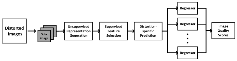
Figure 1: An overview of the proposed GreenBIQA method.

2.3 Green Machine Learning

Green learning [36] has been proposed recently as an alternative machine learning paradigm that targets efficient models of low carbon footprint. They are characterized by small model sizes and low training and inference computational complexities. An additional advantage is its mathematical transparency through a modularized design principle. Green learning was originated by efforts in understanding the functions of various components of CNNs such as nonlinear activation [37], convolutional layers and fully-connected layers [38]. Its development path started to deviate from neural networks by giving up the basic neuron unit and the network architecture since 2020. Examples of green learning models include PixelHop [39] and PixelHop++ [40] for object classification and PointHop [41] and PointHop++ [42] for 3D point cloud classification. Green learning techniques have been developed for many applications such as deepfake detection [43], anomaly detection [44], image generation [45], etc. We propose a lightweight BIQA method in this work by following this path.

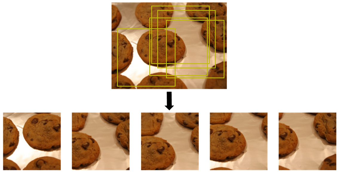
Figure 2: An example of five cropped sub-images for authentic-distortion datasets.

Figure 3: An example of nine cropped sub-images for synthetic-distortion datasets.

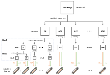
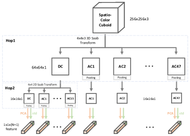
(a) Generation of spatial representations	(b) Generation of joint spatio-color representations

Figure 4: Unsupervised representation generation: spatial representations and joint spatio-color representations.

3 Proposed GreenBIQA Method

An overview of the proposed GreenBIQA method is depicted in Fig. 1. As shown in the figure, GreenBIQA has a modularized solution that consists of five modules: (1) image cropping, (2) unsupervised representation generation, (3) supervised feature selection, (4) distortion-specific prediction, and (5) regression and decision ensemble. They are elaborated below.

3.1 Image Cropping

Image cropping is implemented to standardize the input size and enlarge the number of training samples. It is achieved by cropping sub-images of fixed size from raw images in datasets. All cropped sub-images are assigned the same mean opinion score (MOS) as their source image. To ensure the high correlation between sub-images and their assigned MOS, we adopt different cropping strategies for synthetic-distortion and authentic-distortion datasets as shown in Fig. 2 and Fig. 3, respectively.

For images in authentic-distortion datasets such as KonIQ-10K [46], they contain distortions in unknown regions. Thus, we crop a smaller number of sub-images of a larger size (e.g., $256\times 256$ out of $384\times 512$) to ensure the assigned MOS for each sub-image is reasonable. The cropped sub-images can overlap with one another. Fig. 2 shows five randomly cropped sub-images from one source image.

For images in synthetic-distortion datasets such as KADID-10K [47], all distortions are applied to the reference images uniformly with few exceptions (e.g., color distortion in localized regions in KADID-10K). Only one distortion type is added to one image at a time. Therefore, cropping sub-images of a smaller size is sufficient to capture distortion characteristics. Furthermore, we can crop more sub-images to enlarge the number of training samples and conduct decision ensembles in the inference stage. An example of image cropping from the KADID-10K dataset is shown in Fig. 3, where nine sub-images of size of $64\times 64$ are randomly selected.

3.2 Unsupervised Representation Generation

Given sub-images from the image cropping module, we extract a set of representations from sub-images in an unsupervised manner. We consider two types of representations.

1. Spatial representations. They are extracted from the Y, U, and V channels of sub-images individually.

2. Joint spatio-color representations. They are extracted from a 3D cuboid of size $H\times W\times C$, where $H$ and $W$ are the height and width of a sub-image and $C=3$ is the number of color channels, respectively.

3.2.1 Spatial Representations

Fig. 4 (a) shows the procedure of spatial representation generation. The representations are derived from $8\times 8$ block DCT coefficients since they are often available in compressed images. The input sub-images are first partitioned into non-overlapping blocks of size $8\times 8$ and DCT coefficients are generated by the block DCT transform. DCT coefficients of each block are scanned in the zigzag order, leading to one DC coefficient and 63 AC coefficients, denoted by AC1-AC63. We split them into 64 channels. Generally, the amount of energy decreases from the DC channel to the AC63 channel. There are correlations among DC coefficients of spatially adjacent blocks. We apply the Saab transform [38] to them. The Saab transform uses a constant-element kernel to compute the patch mean, which is called the DC component of the Saab transform. Then, it applies the principal component analysis (PCA) to mean-removed patches in deriving data-driven kernels, called AC kernels. The application of AC kernels to each patch yields AC coefficients of the Saab transform. Here, we decorrelate DC coefficients in two stages, i.e., Hop1 and Hop2.

• Hop1 Processing: We partition $32\times 32$ DC coefficients into non-overlapping blocks of size $4\times 4$ and conduct the Saab transform on each block, leading to one DC channel and 15 AC channels in Hop1. We feed the $8\times 8$ DC coefficients to the next hop.

• HOP2 Processing: We apply another $4\times 4$ Saab transform on each of non-overlapping blocks of size $4\times 4$, leading to DC and 15 AC channels in Hop2. We collect all the representations from Hop2 and append them to the final representation set in preserving low-frequency details.

Other Saab coefficients in Hop1 and other DCT coefficients at the top layer contain mid- and high-frequency information. We need to aggregate them spatially to reduce the representation number. First, we take their absolute values and apply the maximum pooling to lower their dimension as indicated by the down-ward gray arrow. Next, we adopt the following operations to yield two sets of values:

• Compute the maximum value, the mean value, and the standard deviation of the same coefficients across the spatial domain.

• Conduct the PCA transform on spatially adjacent regions for further dimension reduction (except the coefficients in HOP2).

These values are concatenated to form spatial representations of interest. The same process is applied to the Y, U, and V channels of all sub-images.

3.2.2 Joint Spatio-Color Representations

We first convert sub-images from the YUV to RGB color space. The corresponding spatio-color cuboids have a size of $H\times W\times C$, where $H$ and $W$ are the height and width of the sub-image, respectively, and $C=3$ is the number of color channels. They serve as input cuboids to a two-hop hierarchical structure as shown in Fig. 4 (b). In Hop1, we split the input cuboids into non-overlapping cuboids of size $4\times 4\times 3$ and apply the 3D Saab transform to them individually - leading to one DC channel and 47 AC channels, denoted by AC1-AC47. Each channel has a spatial dimension of $64\times 64$. Since the DC coefficients are spatially correlated, we apply the 2D Saab transform in Hop2, where the DC channel of size $64\times 64$ is decomposed into $16\times 16$ non-overlapping blocks of size $4\times 4$. For other 47 AC coefficients in the output of Hop1, we take their absolute values and conduct the 4x4 max pooling, leading to 47 channels of spatial dimension $16\times 16$. In total, we obtain $16+47=63$ channels of the same spatial size $16\times 16$. We use the following two steps to extract joint spatio-color features.

• Flatten blocks to vectors, conduct PCA, and select coefficients from the first $N$ principal components.

• Compute the standard deviation of the coefficients in the same channel.

The above two sets of representations are concatenated to form the joint spatio-color representations.

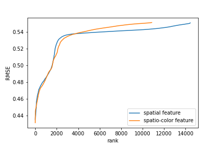
Figure 5: RFT results of spatial and spatio-color representations.

3.3 Supervised Feature Selection

It is desired to select more discriminant features from a large number of representations obtained from the second module. A powerful tool, called the relevant feature test (RFT) [48], is adopted to achieve this objective. It computes the loss of each representation independently. A lower loss value indicates a better representation. To conduct RFT, we split the dynamic range of a representation into two sub-intervals with a set of partition points. For a given partition, we first calculate the means of training samples in its left and right regions respectively as the representative values and compute their mean-squared errors (MSE) accordingly. Then, by combining the MSE values of both regions together, we get the weighted MSE for the partition. Then, we search for the smallest weighted MSE through a set of partition points, and this minimum value defines the cost function of this representation. Note that RFT is a supervised feature selection algorithm since it exploits the label of the training samples. We sort representation indices according to their root-MSE (RMSE) values from the smallest to the largest in Fig. 5. There are two curves, one for the spatial representations and the other for the spatio-color representations. We can use the elbow point on each curve to select a subset of representations. In the experiment, we use RFT to select 2048D spatial features and 2000D spatio-color features. The former is a concatenation of spatial features from Y, U, and V channels.

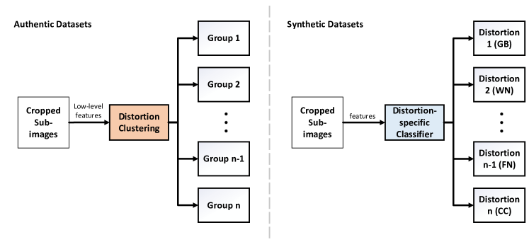
Figure 6: Distortion-specific classifier and distortion clustering for synthetic and authentic datasets, respectively.

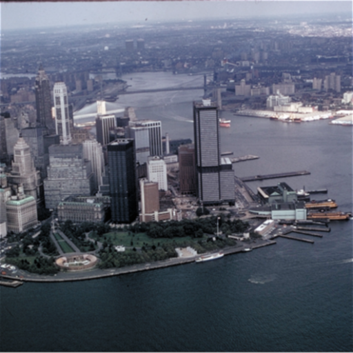
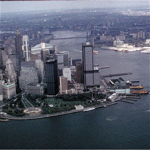
(a)                                         (b)                                         (c)
           
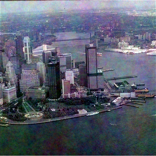
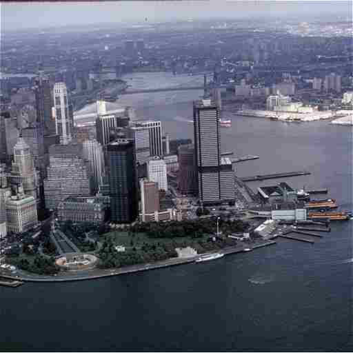
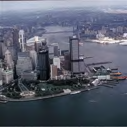
(d)                                         (e)                                         (f)

Figure 7: Six synthetic distortion types in CSIQ: (a) Gaussian blur, (b) Gaussian noise, (c) Contrast decrements, (d) Pink Gaussian noise, (e) JPEG, and (f) JPEG-2000.

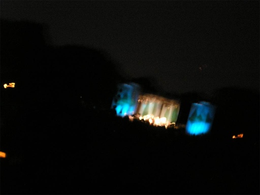
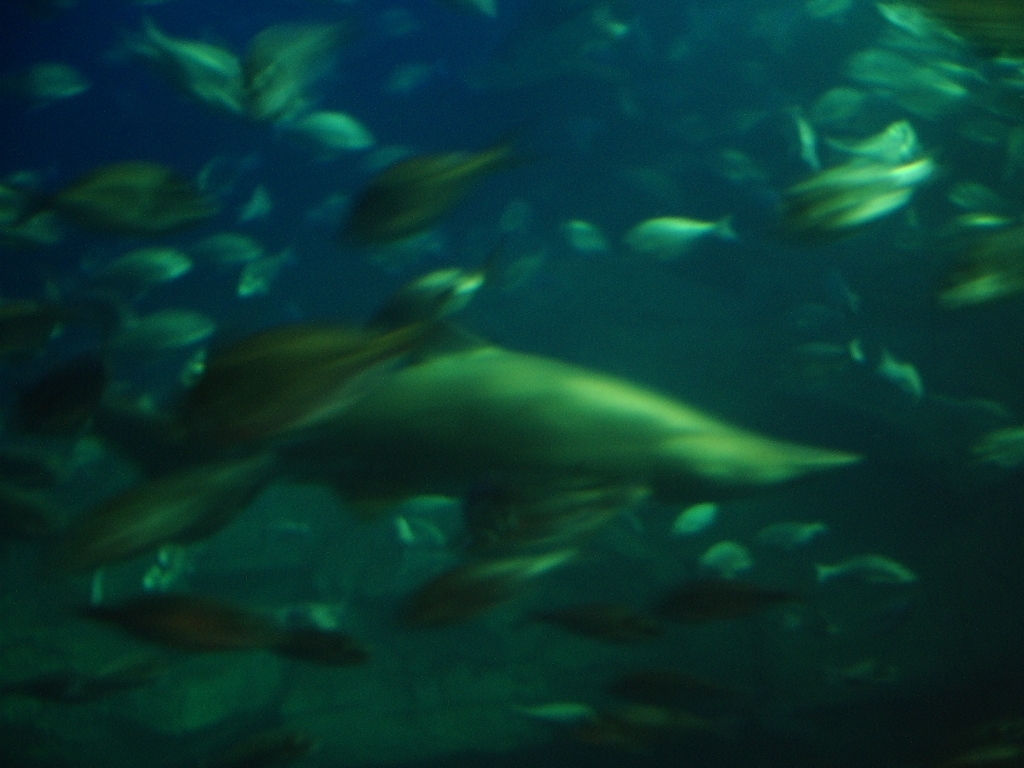
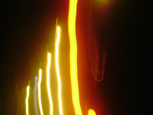
(a)                                             (b)                                             (c)

Figure 8: Three distorted images in KonIQ-10k: (a) Dark environment, (b) Underwater, and (c) Smeared light.

3.4 Distortion-specific Prediction

Usually, we get better prediction scores if we can classify distorted images into several classes based on their distortion types. We examine synthetic-distortion and authentic-distortion datasets separately as shown in Fig. 6 due to their different properties.

3.4.1 Synthetic Distortions

Images in synthetic-distortion datasets are usually associated with one specific distortion type with multiple severity levels. For example, CSIQ [49] has 6 distortion types with 4 to 5 different levels, as shown in Fig. 7. We can leverage the known distortion types by first training a distortion classifier to separate images accordingly. Then, we design an individual pipeline to handle each distortion type. We can use distortion labels of training images to train a multi-class distortion classifier based on the selected features in Sec. 3.3. There are multiple sub-images from one image and each of them may have a different predicted distortion type. We adopt majority voting to determine the image-level distortion type. Note that some distortion types are easily confused with each other (e.g., JPEG and JPEG2000). We can simply merge them into a single type. As a result, the class number can be reduced.

3.4.2 Authentic Distortions

Images from authentic-distortion datasets may contain mixed distortion types introduced in image capture or transmission. Three distorted images from KonIQ-10K are shown in Fig. 8. It is difficult to define each as one specific type. For example, the underwater image contains blurriness, noise, and color distortion. Thus, instead of training a specific-distortion classifier, we cluster images into multiple groups using some low-level features in an unsupervised manner (e.g., the K-means algorithm). The low-level features include statistical information in the spatial and color domains. For spatial features, we apply the Laplacian and Sobel edge filters to all pixels in each sub-image, take their absolute values, and compute the mean, variance, and maximum. For color features, we compute the variance of each color channel (such as Y, U, and V). In addition, higher-order statistics can also be collected as color features. All these extracted features are concatenated into a feature vector for unsupervised clustering. Although unsupervised clustering does not assign a distortion type to a cluster, it reduces the content diversity of sub-images in the same cluster.

3.5 Regression and Decision Ensemble

For each of 6 distortions, 19 distortions, and 4 clusters for CSIQ, KADID-10K, and authentic-distortion datasets, we train an XGBoost regressor  [15] that maps from the feature space to the MOS score, respectively. In the experiment, we set hyper-parameters of the XGBoost regressor to the following: 1) the max depth of each tree is 5, 2) the subsampling ratio is 0.6, 3) the maximum tree number is 2000, and 4) the early stop is adopted. Given the predicted MOS scores of all sub-image from the same source image, a median filter is applied to generate the ultimate predicted MOS score of the input image.

Table 1: Four benchmarking IQA datasets, where the number of distorted images, the number of reference images, the number of distortion types and collection methods of each dataset are listed.

Datasets	Dist.	Ref.	Dist. Types	Scenario
CSIQ	866	30	6	Synthetic
KADID-10K	10,125	81	25	Synthetic
LIVE-C	1,169	N/A	N/A	Authentic
KonIQ-10K	10,073	N/A	N/A	Authentic

4 Experiments

4.1 Experimental Setup

4.1.1 Datasets

We evaluate GreenBIQA on two synthetic IQA datasets and two authentic IQA datasets. Their statistics are given in Table 1. The two synthetic-distortion datasets are CSIQ [49] and KADID-10K [47]. Multiple distortions of various levels are applied to a set of reference images to yield distorted images. CSIQ has six distortion types with four to five distortion levels. KADID-10K contains 25 distortion types with five levels for each distortion type. LIVE-C [50] and KonIQ-10K [46] are two authentic-distortion datasets. They contain a broad range of distorted real-world images captured by users. No reference image and specific distortion type are available for each image. LIVE-C and KonIQ-10K have 1,169 and 10,073 distorted images, respectively.

4.1.2 Benchmarking Methods

We compare the performance of GreenBIQA with nine benchmarking methods in Table 2. They include four conventional and five DL-based BIAQ methods. We divide them into four categories.

• NIQE [17] and BRISQUE [7]. They are conventional BIQA methods using NSS features.

• CORNIA [9] and HOSA [11]. They are conventional BIQA methods using codebooks.

• BIECON [22] and WaDIQaM [23]. They are DL-based BIQA methods without pre-trained models (or simple DL methods).

• PQR [27], DBCNN [29], and HyperIQA [28]. They are DL-based BIAQ methods with pre-trained models (or advanced DL methods).

4.1.3 Evaluation Metrics

The performance is measured by two popular metrics: the Pearson Linear Correlation Coefficient (PLCC) and the Spearman Rank Order Correlation Coefficient (SROCC). PLCC evaluates the correlation between predicted scores from an objective method and user’s subjective scores (e.g., MOS) in form of

$$\textit{PLCC}=1-\frac{\sum_{i}(p_{i}-p_{m})(\hat{p_{i}}-\hat{p_{m}})}{\sqrt{\sum_{i}(p_{i}-p_{m})^{2}}\sqrt{\sum_{i}\hat{p_{i}}-\hat{p_{m}})^{2}}},$$ (1)

where $p_{i}$ and $\hat{p_{i}}$ represent predicted and subjective scores while $p_{m}$ and $\hat{p_{m}}$ are their means, respectively. SROCC measures the monotonicity between predicted scores from an objective method and user’s subjective scores via

$$\textit{SROCC}=1-\frac{6\sum_{i=1}^{L}(m_{i}-n_{i})^{2}}{L(L^{2}-1)},$$ (2)

where $m_{i}$ and $n_{i}$ denote the ranks of the prediction and the ground truth label, respectively, and $L$ denotes the total number of samples or the number of images in our current case.

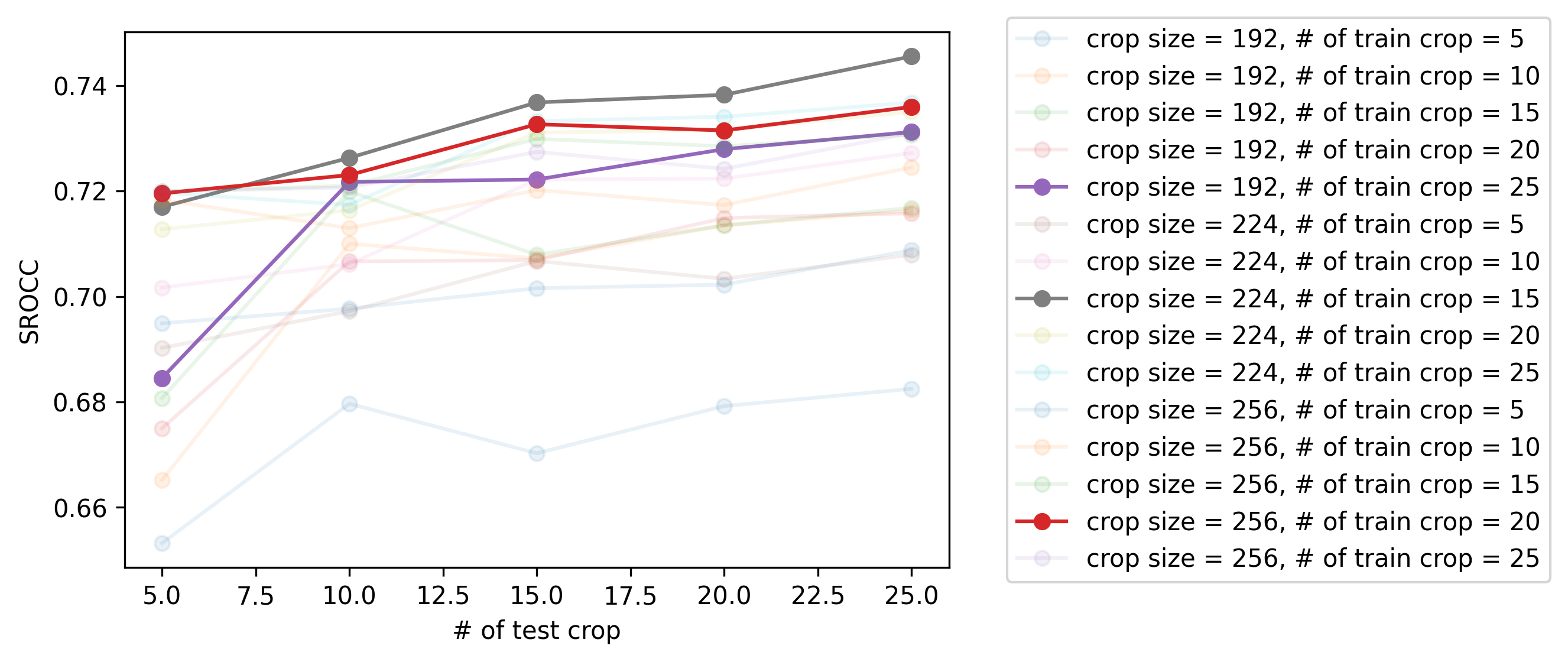
Figure 9: Performance curve on the validation dataset of LIVE-C with different crop numbers and sizes.

4.1.4 Implementation Details

In the training stage, we crop 15 sub-images of size $224\times 224$ for each image in the two authentic datasets. This design choice is based on SROCC performance of validation sets as shown in Fig. 9, where the best performance under different crop sizes is highlighted. Similarly, we crop 25 sub-images of size $32\times 32$ for each image in the two synthetic datasets. In the testing (or inference) stage, we crop 25 sub-images of size $224\times 224$ and $32\times 32$ for images in authentic and synthetic datasets, respectively.

We adopt the standard evaluation procedure by splitting each dataset into 80% for training and 20% for testing. Furthermore, 10% of training data is used for validation. We run experiments 10 times and report median PLCC and SROCC values. For synthetic-distortion datasets, splitting is implemented on reference images to avoid content overlap.

4.2 Performance Evalution

We compare the performance of GreenBIQA and nine benchmarking BIQA methods on four IQA datasets in Table 2.

4.2.1 Comparison among Benchmarking Methods

We first compare the performance among the nine benchmarks. Although some conventional BIAQ methods have comparable performance with simple DL methods (without pre-trained models), we see a clear performance gap between conventional BIQA methods and advanced DL methods (with pre-trained models). On the other hand, the model size of advanced DL methods is significantly larger. We comment on the performance of GreenBIQA against other benchmarking methods below.

4.2.2 Synthetic-Distortion Datasets

For the two synthetic-distortion datasets, CSIQ and KADID-10K, GreenBIQA achieves the best performance among all. This is attributed to its two characteristics: 1) classification of synthetic distortions to multiple types followed by different processing pipelines, and 2) effective usage of ensemble decisions. For the first point, there are six distortion types in CSIQ as shown in Fig. 7. We show the SROCC performance of the best BIQA method in each of four categories against each of six distortion types in the CSIQ dataset in Table 3. GreenBIAQ outperforms all others in four distortion types. It performs especially well for JPEG distortion because it adopts the DCT spatial features which match the underlying compression distortion well. GreenBIQA is also effective against white Gaussian noise (WN), pink Gaussian noise (FN), and contrast decrements (CC) through the use of joint spatial and spatio-color features. GreenBIQA still works well for Gaussian blur (GB) although no blur detector is employed. For the second point, since the number of reference images is limited and the distortion is uniformly spread out across the whole image, ensemble decision works well in such a setting.

Table 2: Performance comparison in PLCC and SROCC metrics between our GreenBIQA method and nine benchmarking methods on four IQA databases, where the nine benchmarking methods are categorized into four groups as discussed in Sec. 4.1 and the best performance numbers are shown in boldface.

	CSIQ		LIVE-C		KADID-10K		KonIQ-10K
Model	SROCC	PLCC	SROCC	PLCC	SROCC	PLCC	SROCC	PLCC	Model size (MB)
NIQE	0.627	0.712	0.455	0.483	0.374	0.428	0.531	0.538	-
BRISQUE	0.746	0.829	0.608	0.629	0.528	0.567	0.665	0.681	-
CORNIA	0.678	0.776	0.632	0.661	0.516	0.558	0.780	0.795	7.4
HOSA	0.741	0.823	0.661	0.675	0.618	0.653	0.805	0.813	0.23
BIECON	0.815	0.823	0.595	0.613	-	-	0.618	0.651	35.2
WaDIQaM	0.844	0.852	0.671	0.680	-	-	0.797	0.805	25.2
PQR	0.872	0.901	0.857	0.882	-	-	0.880	0.884	235.9
DBCNN	0.946	0.959	0.851	0.869	0.851	0.856	0.875	0.884	54.6
HyperIQA	0.923	0.942	0.859	0.882	0.852	0.845	0.906	0.917	104.7
GreenBIQA (Ours)	0.952	0.959	0.801	0.809	0.886	0.893	0.858	0.870	1.82

Table 3: Comparison of the SROCC performance for each of six individual distortion types in the CSIQ dataset, where WN, JPEG, JP2K, FN, GB, and CC denote white Gaussian noise, JPEG compression, JPEG-2000 compression, pink Gaussian noise, Gaussian blur, contrast decrements, respectively. The last column shows the weighted average of the SROCC metrics.

	WN	JPEG	JP2K	FN	GB	CC	Average
BRISQUE	0.723	0.806	0.840	0.378	0.820	0.804	0.728
HOSA	0.604	0.733	0.818	0.500	0.841	0.716	0.702
BIECON	0.902	0.942	0.954	0.884	0.946	0.523	0.858
HyperIQA	0.927	0.934	0.960	0.931	0.915	0.874	0.923
GreenBIQA (Ours)	0.943	0.980	0.969	0.965	0.894	0.857	0.934

4.2.3 Authentic-Distortion Datasets

For the two authentic-distortion datasets, LIVE-C and KonIQ-10K, GreenBIQA outperforms conventional BIQA methods and simple DL methods. This demonstrates the effectiveness of its extracted quality-aware features and decision pipeline in handling diversified distortions and contents. There is however a performance gap between GreenBIQA and advanced DL methods with pre-trained models. The authentic-distortion datasets are more challenging because of non-uniform distortions across images and a wide variety of content without duplication. Since pre-trained models are trained by a much larger image database, they have advantages in extracting features for non-uniform distortions and unseen contents. Yet, they demand much larger model sizes as a tradeoff.

4.3 Cross-Domain Learning

To evaluate transferability of BIQA methods, we train models on one dataset and test them on another dataset. Due to the huge differences in synthetic-distortion and authentic-distortion datasets, we focus on authentic-distortion datasets and conduct experiments on LIVE-C and KonIQ-10K only. We consider two experimental settings: I) trained with LIVE-C and tested on KonIQ-10K, and II) trained with KonIQ-10K and tested on LIVE-C. The SROCC performance of GreenBIQA and five benchmarking methods under the two settings are compared in Table 4, where benchmarks include the three best BIQA methods in Table 2 (i.e. PQR, DBCNN, and HyperIQA) and two conventional BIQA methods (i.e. BRISQUE and HOSA). By comparing the performance numbers in Tables 2 and 4, we see a performance drop in the cross-domain condition for all methods. We see that GreenBIQA has a performance gap of 0.019 and 0.053 against the best one, HyperIQA, for Experimental Settings I and II, respectively. As shown in Table 1, KonIQ-10K is much larger than LIVE-C. Experimental Setting I provides a more proper environment to demonstrate the robustness (or generalizability) of a learning model. We compare the performance gaps in Table 4 under Setting I with those in the KonIQ-10K/SROCC column in Table 2. The gaps between PQR, DBCNN, HyperIQA, and GreenBIQA narrow down from 0.022, 0.017, and 0.048 to 0.004, 0.001, and 0.019, respectively. We see a greater potential of GreenBIQA along this direction.

Table 4: Comparison of the SROCC performance under the cross-domain learning scenario.

Settings	I	II
Train Dataset	LIVE-C	KonIQ-10K
Test Dataset	KonIQ-10K	LIVE-C
BRISQUE	0.425	0.526
HOSA	0.651	0.648
PQR	0.757	0.770
DBCNN	0.754	0.755
HyperIQA	0.772	0.785
GreenBIQA(Ours)	0.753	0.732

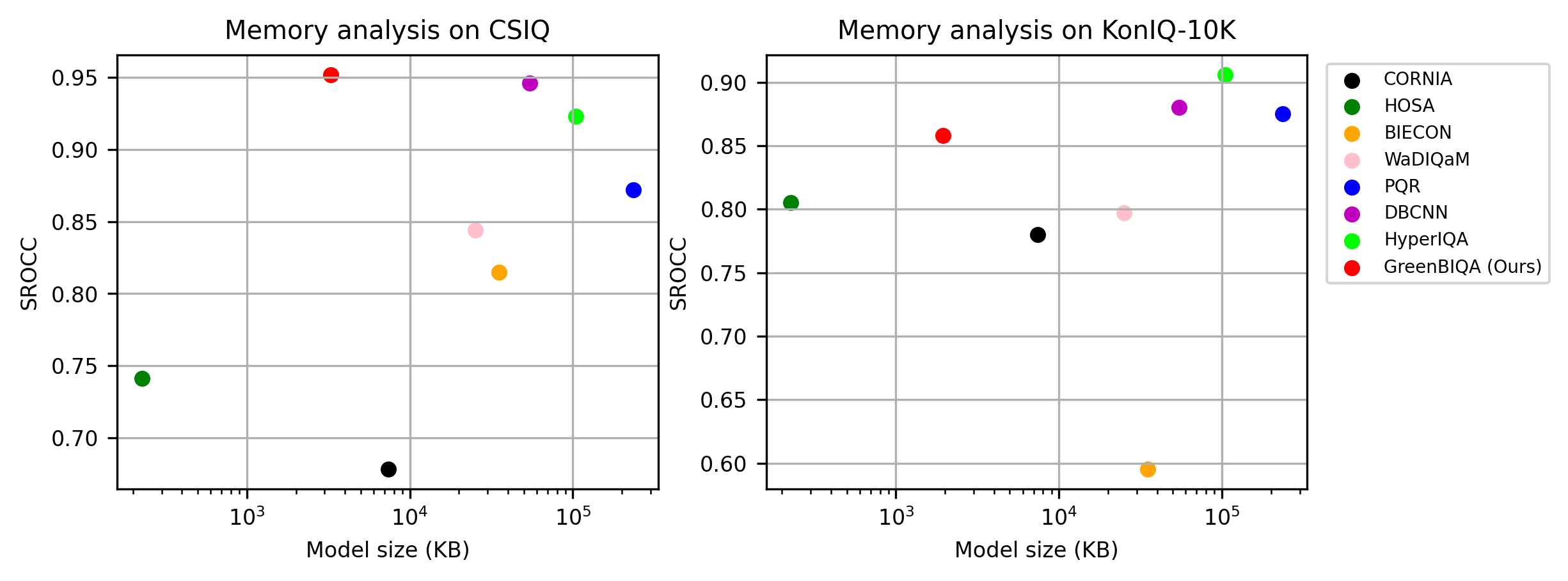
(a) The SROCC performance versus the model size

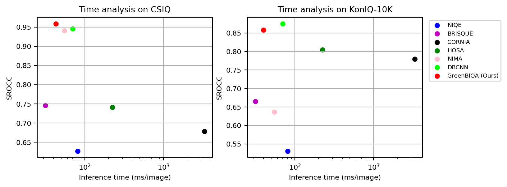
(b) The SROCC performance versus the running time

Figure 10: Illustration of the tradeoff between (a) the SROCC performance and model sizes and (b) the SROCC performance and running time with respect to CSIQ and KonIQ-10K datasets among several BIQA methods.

4.4 Model Complexity

A lightweight model is critical to applications on mobile and edge devices. We analyze the model complexity of BIQA methods in four aspects below: model sizes, inference time, computational complexity in terms of floating-point operations (FLOPs), and memory/latency tradeoff.

4.4.1 Model Size

There are two ways to measure the size of a learning model: 1) the number of model parameters and 2) the actual memory usage. Floating-point and integer model parameters are typically represented by 4 bytes and 2 bytes, respectively. Since a great majority of model parameters are in floating point, the actual memory usage is roughly equal to $4\times\mbox{(no. of model parameters)}$ bytes (see Table 5). To avoid confusion, we use the “model size" to refer to actual memory usage below. Fig. 10(a) plots the SROCC performance (in linear scale along the vertical axis) versus model sizes (in log scale along the horizontal axis) on a synthetic-distortion dataset (i.e., CSIQ) and an authentic-distortion dataset, (i.e., KonIQ-10K) with respect to a few benchmarking BIQA methods. The size of the GreenBIQA model includes: the feature extractor (600KB), the distortion-specific classifier (50KB) and several regressors (1.17MB), leading to a total of 1.82 MB. As compared with the two conventional methods (CORINA and HOSA), GreenBIQA achieves much better performance with comparable model sizes. GreenBIQA outperforms two simple DL methods (BIECON and WaDIQaM), with a smaller model size. As compared with the three advanced DL methods (PQR, DBCNN and HyperIQA), GreenBIQA achieves the best performance on CSIQ and competitive performance on KonIQ-10k at a significantly smaller model size. Note that advanced DL methods have a huge pre-trained network of size larger than 100MB as their backbones.

4.4.2 Inference Time

Another important factor to consider is running time in inference, which is especially the case for mobile/edge clients. Fig. 10(b) shows the SROCC performance versus the inference time (measured in milliseconds per image) for several benchmarking methods on CSIQ and KonIQ-10K. All methods are tested in the same environment with a single CPU. We compare GreenBIQA with four conventional methods (NIQE, BRISQUE, CORNIA, and HOSA) and two DL methods (NIMA and DBCNN). GreenBIQA has clear advantages over all benchmarking methods by considering the performance and inference time jointly. It is worthwhile to point out that GreenBIQA can process around 43 images per second with a single CPU. In other words, it can meet the real-time requirement by processing videos of 30 fps on a frame-by-frame basis. The inference time of GreenBIQA can be further reduced by code optimization and/or with the support of mature packages.

Table 5: Comparison of SROCC/PLCC performance, no. of model parameters, model sizes (memory usage), no. of GigaFlops and no. of KiloFlops per pixel of several BIQA methods tested on the LIVE-C dataset, where “X" denotes the multiple no.

Model	SROCC	PLCC	Model Parameters (M)	Model Size (MB)	GFLOPs	KFLOPs/pixel
NIMA(Inception-v2)	0.637	0.698	10.16 (22.6X)	37.4 (20.5X)	4.37 (128.5X)	87.10 (128.5X)
BIECON	0.595	0.613	7.03 (15.6X)	35.2 (19.3X)	0.088 (2.6X)	85.94 (126.8X)
WaDIQaM	0.671	0.680	5.2 (11.6X)	25.2 (13.8X)	0.137 (4X)	133.82 (197.4X)
DBCNN	0.851	0.869	14.6 (32.4X)	54.6 (30X)	16.5 (485.3)	328.84 (485.1X)
HyerIQA	0.859	0.882	28.3 (62.9X)	104.7 (57.5X)	12.8 (376.5X)	255.10 (376.3X)
GreenBIQA (Ours)	0.801	0.809	0.45(1X)	1.82(1X)	0.034 (1X)	0.678(1X)

4.4.3 Computational Complexity

We compare the SROCC and PLCC performance, the numbers of model parameters, model sizes (in terms of memory usage), the numbers of Flops and Flops per pixel of several BIQA methods tested on the LIVE-C dataset in Table 5. FLOPs is a common metric to measure the computational complexity of a model. For a given hardware configuration, the number of FLOPs is linearly proportional to energy consumption or carbon footprint. Column “GFLOPs" in Table 5 gives the number of GFLOPs needed to run a model once without considering the patch number and size used in a method. For a fair comparison of FLOPs, we compute the number of FLOPS per pixel defined by

$$FLOPs/pixel=\frac{FLOPs/patch}{H\times W},$$ (3)

where $H$ and $W$ are the height and width of an input patch to a model, respectively. NIMA with the pre-trained Inception-v2 network has low performance, large model size, and high complexity. Although simple DL methods (e.g., WaDIQaM and BIECON) use smaller networks with lower FLOPs, their performance is still inferior to GreenBIQA. Finally, advanced DL methods (e.g., DBCNN and HyperIQA) outperform GreenBIQA in SROCC and PLCC performance. However, their model sizes are much larger and their computational complexities are much higher. The numbers of FLOPs of DBCNN and HyperIQA are 485 and 376 multiples of that of GreenBIQA, respectively.

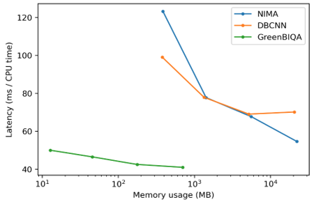
Figure 11: Tradeoff between memory usage and latency for three BIQA methods (NIMA, DBCNN and GreenBIQA), where latency can be reduced by the usage of a larger memory.

4.4.4 Memory/Latency Tradeoff

There is a tradeoff between memory usage and latency in the image quality inference stage. That is, latency can be reduced when given more computing resources. To observe the tradeoff, we control the memory usage using different test image numbers in each run (i.e. the batch size). Fig. 11 shows the latency (in linear scale along the vertical axis) and memory usage (in log scale along the horizontal axis) of GreenBIQA and two advanced DL methods, where we set the batch size equal to 1, 4, 16, and 64 in four experiments. We see from the figure that the latency of GreenBIQA is much smaller than NIMA and DBCNN under the same memory size (say, $10^{3}$MB). Along this line, the memory requirement of GreenBIQA is much lower than that of NIMA and DBCNN at the same level of latency. Again, the memory/latency tradeoff curve of GreenBIQA can be further improved through code optimization.

Table 6: Ablation Study for GreenBIQA.

	CSIQ		LIVE-C		KADID-1K		KonIQ-10k
Components	SROCC	PLCC	SROCC	PLCC	SROCC	PLCC	SROCC	PLCC
S-features	0.925	0.936	0.774	0.778	0.847	0.848	0.822	0.838
S-features + SC-features	-	-	0.782	0.783	-	-	0.835	0.850
S-features + Dist-predict	0.952	0.959	0.786	0.788	0.886	0.893	0.839	0.856
S-features + SC-features + Dist-predict	-	-	0.801	0.809	-	-	0.858	0.870

4.5 Ablation Study

To understand the impact of individual components on the overall performance of GreenBIQA, we conduct an ablation study in Table 6, where S-features, SC-features, and Dist-predict denotes spatial features, spatio-color features, and distortion-specific prediction, respectively. We first examine the effectiveness of the spatial features and then add spatio-color features in the first two rows. Both SROCC and PLCC improve on the two authentic-distortion datasets. Similarly, adding distortion-specific prediction to S-features can improve SROCC and PLCC for all datasets in the third row. Finally, we use all the components in the fourth row and see that SROCC and PLCC can be further improved to reach the highest value. Note that we do not report the performance of joint spatial and spatio-color features for synthetic datasets since spatial features are powerful enough. The distortion-specific prediction benefits the performance significantly on synthetic datasets by leveraging the distortion label.

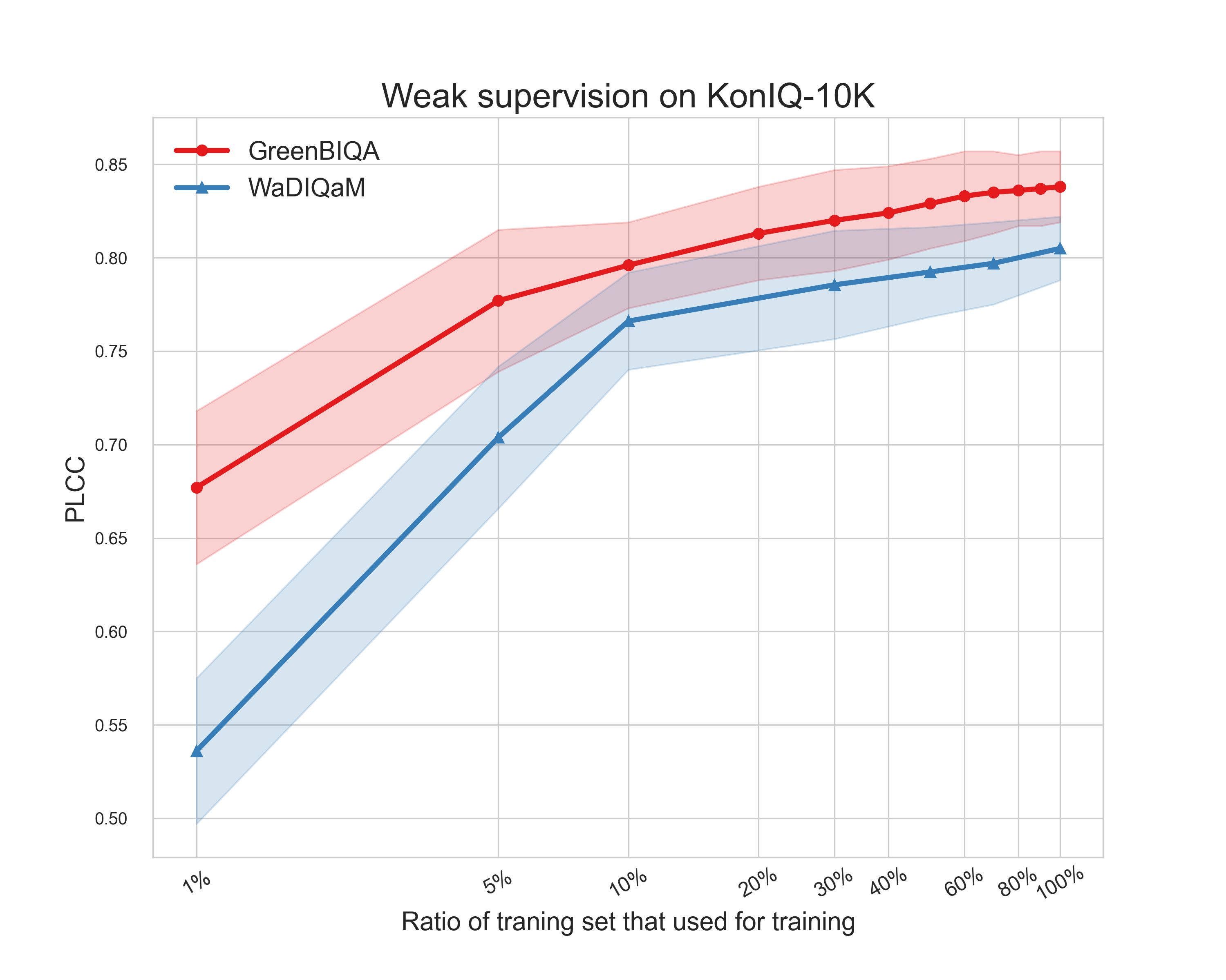
Figure 12: The PLCC performance curves of GreenBIQA and WaDIQaM are plotted as functions of the percentages of the full training dataset of KonIQ-10K, where the solid line and the banded structure indicate the mean value and the range of mean plus/minus one standard deviation, respectively.

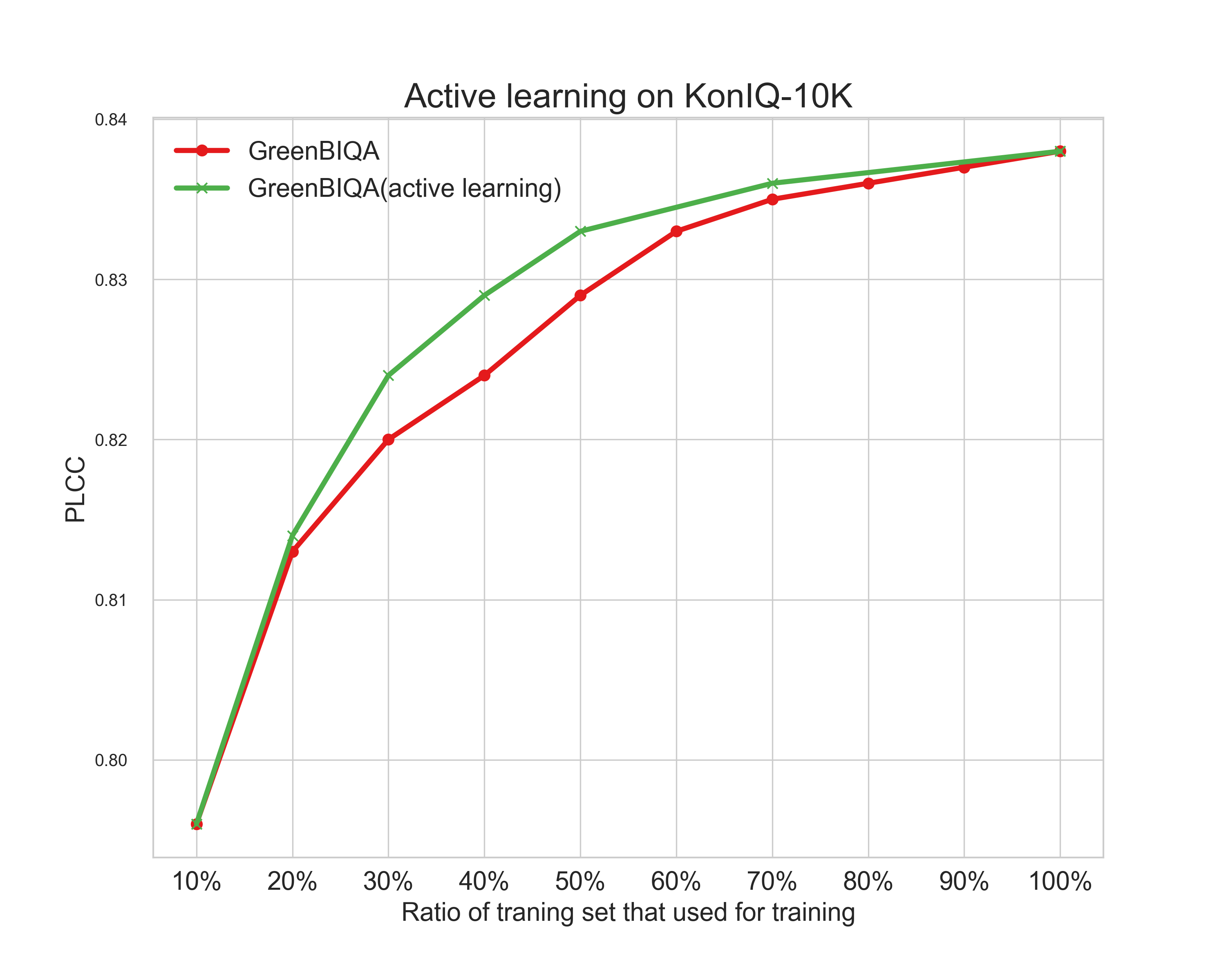
Figure 13: Comparison of the PLCC performance of GreenBIQA using active learning (in green) and random selection (in red) on the KonIQ-10k dataset.

4.6 Weak Supervision

We train BIQA models using different percentages of the KonIQ-10K training dataset (e.g. from 1% to 90%) as shown in Fig. 12 and show the PLCC performance against the full test dataset. For a fair comparison, we only compare GreenBIQA with WaDIQaM, which is a simple DL method. Note that we do not choose advanced DL methods with pre-trained networks for performance benchmarking since pre-trained networks have been trained by other larger datasets. We show the mean and the plus/minus one standard deviation. We see that GreenBIQA performs robustly under the weak supervision setting. Even if it is only trained on 1% of training samples, GreenBIQA can achieve a PLCC value higher than 0.67. Conversely, WaDIQaM does not perform well when the percentage goes low since a small number of samples is not sufficient in the training of a large neural network.

4.7 Active Learning

To further investigate the potential of GreenBIQA, we implement an active learning scheme [51, 52] below.

1. Keep the initial training set as 10% of the full training dataset and obtain an initial model denoted by $M_{1}$.

2. Predict the performance of remaining samples in the training dataset using $M_{i}$, $i=1,2,\cdots,8$. Compute the standard derivation of predicted scores of all sub-images associated with the same image, which indicates prediction uncertainty.

3. Select a set of images that have the highest standard derivations in Step 2, where its size is 10% of the full training dataset. Merge them into the current training image set; namely, their ground truth labels are leveraged to train Model $M_{i+1}$.

We repeat the above process in sequence to obtain models $M_{1},\cdots,M_{9}$. Model $M_{10}$ is the same as the one that uses all training samples. We compare the PLCC performance of GreenBIQA with active learning and with random sampling in Fig. 13. We see that the active learning strategy can improve the performance of the random selection scheme in the range from 20% to 70% of full training samples.

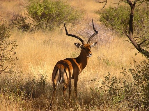
MOS(G) = 3.63	MOS(G) = 3.72	MOS(G) = 4.21	MOS(G) = 1.78
MOS(P) = 3.65	MOS(P) = 3.81	MOS(P) = 3.75	MOS(P) = 2.68

Figure 14: Comparison of the ground truth MOS and Green-BIQA predicted MOS values of four exemplary images, which are represented by MOS(G) and MOS(P), respectively.

5 Conclusion and Future Work

A lightweight high-performance blind image quality assessment method, called GreenBIQA, was presented in this paper. Its PLCC and SROCC performance was evaluated on two synthetic-distortion datasets and two authentic-distortion datasets. It outperforms all conventional BIQA methods and simple DL methods in all four datasets. As compared to the state-of-the-art advanced DL methods with pre-trained models, GreenBIQA still has the best performance in synthetic datasets and offers close-to-best performance in authentic datasets. Above all, GreenBIQA has tremendous advantages in its small model sizes, fast inference time, and low computational complexities (in terms of FLOPs). These properties make GreenBIQA an ideal BIQA choice in mobile and edge devices.

There are several research topics worth further investigation. First, we show four exemplary images with their ground truth and GreenBIQA predicted MOS values in Fig. 14. The left two give good prediction scores while the right two illustrate poor prediction scores. GreenBIQA underestimates the MOS score of the long-horn deer image due to the blurred background. GreenBIQA overestimates the MOS score of the light tower image due to lack of sufficient training samples of similar characteristics. To further improve the performance of GreenBIQA, we need a low-cost mechanism to find the attention region and/or a way to check the prediction confidence. Second, it is important to generalize GreenBIQA to lightweight high-performance video quality assessment by incorporating temporal information.

References

- [1] Zhou Wang, Alan C Bovik, Hamid R Sheikh, and Eero P Simoncelli. Image quality assessment: from error visibility to structural similarity. IEEE transactions on image processing, 13(4):600–612, 2004.
- [2] Lin Zhang, Lei Zhang, Xuanqin Mou, and David Zhang. Fsim: A feature similarity index for image quality assessment. IEEE transactions on Image Processing, 20(8):2378–2386, 2011.
- [3] Tsung-Jung Liu, Weisi Lin, and C-C Jay Kuo. Image quality assessment using multi-method fusion. IEEE Transactions on image processing, 22(5):1793–1807, 2012.
- [4] Abdul Rehman and Zhou Wang. Reduced-reference image quality assessment by structural similarity estimation. IEEE transactions on image processing, 21(8):3378–3389, 2012.
- [5] Anush Krishna Moorthy and Alan Conrad Bovik. A two-step framework for constructing blind image quality indices. IEEE Signal processing letters, 17(5):513–516, 2010.
- [6] Michele A Saad, Alan C Bovik, and Christophe Charrier. Blind image quality assessment: A natural scene statistics approach in the dct domain. IEEE transactions on Image Processing, 21(8):3339–3352, 2012.
- [7] Anish Mittal, Anush Krishna Moorthy, and Alan Conrad Bovik. No-reference image quality assessment in the spatial domain. IEEE Transactions on image processing, 21(12):4695–4708, 2012.
- [8] Peng Ye and David Doermann. No-reference image quality assessment using visual codebooks. IEEE Transactions on Image Processing, 21(7):3129–3138, 2012.
- [9] Peng Ye, Jayant Kumar, Le Kang, and David Doermann. Unsupervised feature learning framework for no-reference image quality assessment. In 2012 IEEE conference on computer vision and pattern recognition, pages 1098–1105. IEEE, 2012.
- [10] Lin Zhang, Zhongyi Gu, Xiaoxu Liu, Hongyu Li, and Jianwei Lu. Training quality-aware filters for no-reference image quality assessment. IEEE MultiMedia, 21(4):67–75, 2014.
- [11] Jingtao Xu, Peng Ye, Qiaohong Li, Haiqing Du, Yong Liu, and David Doermann. Blind image quality assessment based on high order statistics aggregation. IEEE Transactions on Image Processing, 25(9):4444–4457, 2016.
- [12] Jia Deng, Wei Dong, Richard Socher, Li-Jia Li, Kai Li, and Li Fei-Fei. Imagenet: A large-scale hierarchical image database. In 2009 IEEE conference on computer vision and pattern recognition, pages 248–255. Ieee, 2009.
- [13] Zhanxuan Mei, Yun-Cheng Wang, Xingze He, and C-C Jay Kuo. Greenbiqa: A lightweight blind image quality assessment method. In 2022 IEEE 24th International Workshop on Multimedia Signal Processing (MMSP), pages 1–6. IEEE, 2022.
- [14] Mariette Awad and Rahul Khanna. Support vector regression. In Efficient learning machines, pages 67–80. Springer, 2015.
- [15] Tianqi Chen and Carlos Guestrin. Xgboost: A scalable tree boosting system. In Proceedings of the 22nd acm sigkdd international conference on knowledge discovery and data mining, pages 785–794, 2016.
- [16] Anush Krishna Moorthy and Alan Conrad Bovik. Blind image quality assessment: From natural scene statistics to perceptual quality. IEEE transactions on Image Processing, 20(12):3350–3364, 2011.
- [17] Anish Mittal, Rajiv Soundararajan, and Alan C Bovik. Making a completely blind image quality analyzer. IEEE Signal processing letters, 20(3):209–212, 2012.
- [18] Fu-Zhao Ou, Yuan-Gen Wang, and Guopu Zhu. A novel blind image quality assessment method based on refined natural scene statistics. In 2019 IEEE International Conference on Image Processing (ICIP), pages 1004–1008. IEEE, 2019.
- [19] Wufeng Xue, Xuanqin Mou, Lei Zhang, Alan C Bovik, and Xiangchu Feng. Blind image quality assessment using joint statistics of gradient magnitude and laplacian features. IEEE Transactions on Image Processing, 23(11):4850–4862, 2014.
- [20] Lin Zhang, Lei Zhang, and Alan C Bovik. A feature-enriched completely blind image quality evaluator. IEEE Transactions on Image Processing, 24(8):2579–2591, 2015.
- [21] Le Kang, Peng Ye, Yi Li, and David Doermann. Convolutional neural networks for no-reference image quality assessment. In Proceedings of the IEEE conference on computer vision and pattern recognition, pages 1733–1740, 2014.
- [22] Jongyoo Kim and Sanghoon Lee. Fully deep blind image quality predictor. IEEE Journal of selected topics in signal processing, 11(1):206–220, 2016.
- [23] Sebastian Bosse, Dominique Maniry, Klaus-Robert Müller, Thomas Wiegand, and Wojciech Samek. Deep neural networks for no-reference and full-reference image quality assessment. IEEE Transactions on image processing, 27(1):206–219, 2017.
- [24] Kede Ma, Wentao Liu, Kai Zhang, Zhengfang Duanmu, Zhou Wang, and Wangmeng Zuo. End-to-end blind image quality assessment using deep neural networks. IEEE Transactions on Image Processing, 27(3):1202–1213, 2017.
- [25] Kaiming He, Xiangyu Zhang, Shaoqing Ren, and Jian Sun. Deep residual learning for image recognition. In Proceedings of the IEEE conference on computer vision and pattern recognition, pages 770–778, 2016.
- [26] Hui Zeng, Lei Zhang, and Alan C Bovik. A probabilistic quality representation approach to deep blind image quality prediction. arXiv preprint arXiv:1708.08190, 2017.
- [27] Hui Zeng, Lei Zhang, and Alan C Bovik. Blind image quality assessment with a probabilistic quality representation. In 2018 25th IEEE International Conference on Image Processing (ICIP), pages 609–613. IEEE, 2018.
- [28] Shaolin Su, Qingsen Yan, Yu Zhu, Cheng Zhang, Xin Ge, Jinqiu Sun, and Yanning Zhang. Blindly assess image quality in the wild guided by a self-adaptive hyper network. In Proceedings of the IEEE/CVF Conference on Computer Vision and Pattern Recognition, pages 3667–3676, 2020.
- [29] Weixia Zhang, Kede Ma, Jia Yan, Dexiang Deng, and Zhou Wang. Blind image quality assessment using a deep bilinear convolutional neural network. IEEE Transactions on Circuits and Systems for Video Technology, 30(1):36–47, 2018.
- [30] Kwan-Yee Lin and Guanxiang Wang. Hallucinated-iqa: No-reference image quality assessment via adversarial learning. In Proceedings of the IEEE conference on computer vision and pattern recognition, pages 732–741, 2018.
- [31] Ian Goodfellow, Jean Pouget-Abadie, Mehdi Mirza, Bing Xu, David Warde-Farley, Sherjil Ozair, Aaron Courville, and Yoshua Bengio. Generative adversarial networks. Communications of the ACM, 63(11):139–144, 2020.
- [32] Hossein Talebi and Peyman Milanfar. Nima: Neural image assessment. IEEE transactions on image processing, 27(8):3998–4011, 2018.
- [33] Karen Simonyan and Andrew Zisserman. Very deep convolutional networks for large-scale image recognition. arXiv preprint arXiv:1409.1556, 2014.
- [34] Christian Szegedy, Vincent Vanhoucke, Sergey Ioffe, Jon Shlens, and Zbigniew Wojna. Rethinking the inception architecture for computer vision. In Proceedings of the IEEE conference on computer vision and pattern recognition, pages 2818–2826, 2016.
- [35] Andrew G Howard, Menglong Zhu, Bo Chen, Dmitry Kalenichenko, Weijun Wang, Tobias Weyand, Marco Andreetto, and Hartwig Adam. Mobilenets: Efficient convolutional neural networks for mobile vision applications. arXiv preprint arXiv:1704.04861, 2017.
- [36] C-C Jay Kuo and Azad M Madni. Green learning: Introduction, examples and outlook. Journal of Visual Communication and Image Representation, 90:103685, 2023.
- [37] C-C Jay Kuo. Understanding convolutional neural networks with a mathematical model. Journal of Visual Communication and Image Representation, 41:406–413, 2016.
- [38] C-C Jay Kuo, Min Zhang, Siyang Li, Jiali Duan, and Yueru Chen. Interpretable convolutional neural networks via feedforward design. Journal of Visual Communication and Image Representation, 60:346–359, 2019.
- [39] Yueru Chen and C-C Jay Kuo. Pixelhop: A successive subspace learning (SSL) method for object recognition. Journal of Visual Communication and Image Representation, page 102749, 2020.
- [40] Yueru Chen, Mozhdeh Rouhsedaghat, Suya You, Raghuveer Rao, and C-C Jay Kuo. Pixelhop++: A small successive-subspace-learning-based (SSL-based) model for image classification. In 2020 IEEE International Conference on Image Processing (ICIP), pages 3294–3298. IEEE, 2020.
- [41] Min Zhang, Haoxuan You, Pranav Kadam, Shan Liu, and C-C Jay Kuo. Pointhop: An explainable machine learning method for point cloud classification. IEEE Transactions on Multimedia, 2020.
- [42] Min Zhang, Yifan Wang, Pranav Kadam, Shan Liu, and C-C Jay Kuo. Pointhop++: A lightweight learning model on point sets for 3d classification. arXiv preprint arXiv:2002.03281, 2020.
- [43] Hong-Shuo Chen, Mozhdeh Rouhsedaghat, Hamza Ghani, Shuowen Hu, Suya You, and C-C Jay Kuo. Defakehop: A light-weight high-performance deepfake detector. In 2021 IEEE International Conference on Multimedia and Expo (ICME), pages 1–6. IEEE, 2021.
- [44] Kaitai Zhang, Bin Wang, Wei Wang, Fahad Sohrab, Moncef Gabbouj, and C-C Jay Kuo. Anomalyhop: an ssl-based image anomaly localization method. In 2021 International Conference on Visual Communications and Image Processing (VCIP), pages 1–5. IEEE, 2021.
- [45] Xuejing Lei, Ganning Zhao, Kaitai Zhang, and C-C Jay Kuo. Tghop: an explainable, efficient, and lightweight method for texture generation. APSIPA Transactions on Signal and Information Processing, 10:e17, 2021.
- [46] Vlad Hosu, Hanhe Lin, Tamas Sziranyi, and Dietmar Saupe. Koniq-10k: An ecologically valid database for deep learning of blind image quality assessment. IEEE Transactions on Image Processing, 29:4041–4056, 2020.
- [47] Hanhe Lin, Vlad Hosu, and Dietmar Saupe. Kadid-10k: A large-scale artificially distorted iqa database. In 2019 Eleventh International Conference on Quality of Multimedia Experience (QoMEX), pages 1–3. IEEE, 2019.
- [48] Yijing Yang, Wei Wang, Hongyu Fu, C-C Jay Kuo, et al. On supervised feature selection from high dimensional feature spaces. APSIPA Transactions on Signal and Information Processing, 11(1), 2022.
- [49] Eric Cooper Larson and Damon Michael Chandler. Most apparent distortion: full-reference image quality assessment and the role of strategy. Journal of electronic imaging, 19(1):011006, 2010.
- [50] Deepti Ghadiyaram and Alan C Bovik. Massive online crowdsourced study of subjective and objective picture quality. IEEE Transactions on Image Processing, 25(1):372–387, 2015.
- [51] Mozhdeh Rouhsedaghat, Yifan Wang, Shuowen Hu, Suya You, and C-C Jay Kuo. Low-resolution face recognition in resource-constrained environments. Pattern Recognition Letters, 149:193–199, 2021.
- [52] Burr Settles. Active learning literature survey. 2009.