Matryoshka Policy Gradient for Entropy-Regularized RL: Convergence and Global Optimality

Abstract

A novel Policy Gradient (PG) algorithm, called Matryoshka Policy Gradient (MPG), is introduced and studied, in the context of fixed-horizon max-entropy reinforcement learning, where an agent aims at maximizing entropy bonuses additional to its cumulative rewards. In the function approximation setting with softmax policies, we prove uniqueness and characterize the optimal policy, together with global convergence of MPG. These results are proved in the case of continuous state and action space. MPG is intuitive, theoretically sound and we furthermore show that the optimal policy of the infinite horizon max-entropy objective can be approximated arbitrarily well by the optimal policy of the MPG framework. Finally, we provide a criterion for global optimality when the policy is parametrized by a neural network in terms of the neural tangent kernel at convergence. As a proof of concept, we evaluate numerically MPG on standard test benchmarks.

1 Introduction

1.1 Policy gradient, max-entropy reinforcement learning and fixed horizon

Reinforcement Learning

(RL) tasks can be informally summarized as follows: sequentially, an agent is located at a given state $s$, takes an action $a$, receives a reward $r(a,s)$ and moves to a next state $s^{\prime}\sim p(s,a,\cdot)$, where $p$ is a transition probability kernel. The agent thus seeks to maximize the cumulative rewards from its interactions with the environment, that is, it optimizes its policy $\pi$ by reinforcing decisions that led to high rewards, where $\pi(a|s)$ is the probability for the agent to take action $a$ while at state $s$.

Policy Gradient

(PG) methods are model-free algorithms that aim at solving such RL tasks; model-free refers to the fact that the agent tries to learn (i.e. improve its policy’s performance) without learning the dynamics of the environment governed by $p$, nor the reward function $r$. Though their origins in RL can be dated from several decades ago with the algorithm REINFORCE [42], the name Policy Gradient appearing only in 2000 in [38], they recently regained interest thanks to many remarkable achievements, to name a few: in continuous control [29, 35, 36] and natural language processing with GPT-3 [10]. See the blog post [41] that lists important PG methods and provides a concise introduction to each of them.

Max-entropy RL.

More generally, PG methods are considered more suitable for large (possibly continuous) state and action spaces than other nonetheless important methods such as Q-learning and its variations. However, for large spaces, the exploitation-exploration dilemma becomes more challenging. In order to enhance exploration, it has become standard to use a regularization to the objective, as in max-entropy RL[32, 33, 34], where the agent maximizes the sum of its rewards plus a bonus for the entropy of its policy. Not only max-entropy RL boosts exploration, it also yields an optimal policy that is stochastic, in the form of a Boltzmann measure, such that the agent keeps taking actions at random while maximizing the regularized objective. This is sometimes preferable than deterministic policies. In particular, [16] shows that the max-entropy RL optimal policy is robust to adversarial change of the reward function (their Theorem 4.1) and transition probabilities (their Theorem 4.2); see also references therein for more details on that topic. Finally, max-entropy RL is appealing from a theoretical perspective. For example, soft Q-learning, introduced in [20] (see also [22, 21] for implementations of soft Q-learning with an actor-critic scheme), strongly resembles PG in max-entropy RL [34]; max-entropy RL has also been linked to variational inference in [27]. Other appealing features of max-entropy RL are discussed in [15] and references therein.

Convergence guarantees of PG.

The empirical successes motivated the RL community to build a solid theory for PG methods that is lacking. Indeed, besides the well-known Policy Gradient Theorem (see Chapter 13 in [37]) that can imply convergence of PG (provided good learning rate and other assumptions), for many years, not much more was known about the global convergence of PG (i.e. convergence to an optimal policy) until recently. Despite the numerous gaps that remain, some important progress have already been made. In particular, the global convergence of PG methods has been studied and proved in specific settings, see for instance [17, 1, 7, 30, 43, 44, 11, 13, 40, 2, 8, 26, 19]. Convergence guarantees often come with convergence rates (with or without perfect gradient estimates). Though strengthening the trust in PG methods for practical tasks, most of the theoretical guarantees obtained in the literature so far require rather restrictive assumptions, and often assume that the action-state space of the MDP is finite (but not always, e.g. [2] addresses continuous action-state space for neural policies in the mean-field regime and [26] proves global convergence when adding enough regularization on the parameters.) In particular, [28] shows that many convergence rates that have been obtained in the literature ignore some parameters such as the size of the state space. After making the dependency of the bounds on these parameters explicit, they manage to construct environments where the rates blow up and convergence takes super-exponential time.

Fixed-horizon RL.

A vast number of works on RL have focused on either infinite horizon tasks, or episodic tasks where the length of an episode is random. In both these cases, policies only depend on the current state of the agent. In [14], the fixed, finite horizon optimal policy is used as an approximation, as the horizon grows to infinity, to approximate the infinite-horizon optimal policy. Nonetheless and even though the fixed (deterministic) horizon setting has received less attention, the benefits of fixing the horizon are multiple and have been investigated in recent relevant works, such as [4] and [19]. With a fixed horizon, policies are time-dependent, and are usually called non-stationary policies, as in dynamic programming [6].

The authors in [4] construct a sequence of value and Q-functions to solve a fixed-horizon task. Training is done with a Temporal Difference (TD) algorithm, which is not a PG method. TD involves bootstrapping, and when it is used offline (off-policy) together with function approximation, it encounters the well-known stability issue called the deadly triad, see [37] Section 11.3. By using horizon-dependent value functions, they do not rely on bootstrapping, getting rid of one element of the triad, thus ensuring more stability. It is worth noting that thanks to the fixed-horizon setting, they empirically overcome the specific Baird’s example of divergence.

The preprint [19] exploits a similar idea with an actor-critic method for constrained RL, where the agent aims at maximizing the cumulative rewards while satisfying some given constraints. To guarantee convergence, they assume a condition given by their Equation (20). Roughly speaking, this condition is that smaller horizon policies are closer to convergence than larger horizon policies. Therefore, they prove convergence of the training algorithm through a cascade of convergence, and provide convergence rates.

Let us also mention [39] investigating the impact of the discount factor when optimizing a discounted infinite-horizon objective evaluated on a finite-horizon undiscounted objective. They empirically found that for some tasks, lower discount factors (thus closer to a fixed-horizon objective) lead to better performance.

1.2 Contributions

We consider the function approximation setting with log-linear parametric policies, that are constructed as the softmax of linear models. The main contributions of this work are:

1. We define the fixed-horizon max-entropy RL objective and introduce a new algorithm (Equation (3.2)), named Matryoshka Policy Gradient (MPG).

2. We establish global convergence for continuous state and action space: under the realizability assumption, MPG converges to the unique optimal policy (Theorem 2). When the realizability assumption does not hold, we prove uniqueness of the optimal policy and prove global convergence of MPG (Theorem 3).

3. We approximate arbitrarily well the optimal policy for the infinite horizon objective by the optimal policy of the MPG objective (Proposition 2).

4. In the case where the policy is parametrized as the softmax of a (deep) neural network’s output, we describe the limit of MPG training in terms of the neural tangent kernel and the conjugate kernel of the neural network at the end of training (Corollary 1). In particular, MPG globally converges in the lazy regime.

5. Numerically, we successfully train agents on standard simple tasks without relying on RL tricks, and confirm our theoretical findings (see Section 4).

In [1], many convergence guarantees are given for different policy gradient algorithms. In particular, in the tabular case with finite state and action space, global convergence is obtained thanks to the gradient domination property. One advantage is that the rate of convergence can be deduced, see e.g. Section 4 in [1]. In the case of infinite state space (and possibly action space, see their Remark 6.8), in the function approximation setting, they obtain convergence results for the natural policy gradient algorithm, which uses the Fisher information matrix induced by the policy in the update, but do not guarantee the optimality of the limit. In contrast, MPG only uses the gradient of the policy and globally converges.

Let us stress the main strength of MPG regarding its convergence guarantees:

1. State space and action space can be continuous.

2. Global convergence is guaranteed in the function approximation setting, independently from the parameters’ initialization.

3. Even when the realizable assumption does not hold, MPG converges to the unique optimal policy in the parametric policy space. We moreover characterise the global optimum as the unique policy satisfying the projectional consistency property.

In our numerical experiments described in Section 4, we first consider an analytical task and verify the global convergence property of the MPG: MPG consistently finds the unique global optimum, which satisfies the projectional consistency property. Then, we study two benchmarks from OpenAI: the Frozen Lake game and the Cart Pole. We obtain successful policies for both benchmarks with a very simple implementation of the MPG algorithm, comparing also to a simple vanilla PG method [38]. Rather than competing with the state-of-the-art algorithms, our aim is to provide a proof of concept by showing that successful training can be obtained without using standard RL tricks that are known to improve training performance. Standard tricks are nevertheless very straightforward to apply to MPG and we hope that more general and bigger scale experiments implementing variations of MPG will follow the present work.

2 Fixed-horizon max-entropy RL

In this section, we introduce the fixed-horizon max-entropy RL, describe its optimal policy and establish some of its properties.

2.1 Definitions

Markov Decision Process

The agent evolves according to a Markov Decision Process (MDP) characterized by the tuple $(\mathcal{S},\mathcal{A},p,p_{\mathrm{rew}})$. The action space can be state dependent $\mathcal{A}_{s}$, nonetheless we assume for simplicity that it is the same regardless of the state. We assume that the action and state spaces $\mathcal{A},\mathcal{S}\subset\mathbb{R}^{d}$ are closed sets. Let $s^{\prime}\mapsto p(s,a,s^{\prime})$ be the probability (the density if $\mathcal{S}$ is continuous) that the agent moves from $s\in\mathcal{S}$ to $s^{\prime}\in\mathcal{S}$ after taking action $a\in\mathcal{A}$. When $p(s,a,s^{\prime})=\delta_{s^{\prime},f(s,a)}$ for some $f:\mathcal{S}\times\mathcal{A}\to\mathcal{S}$, then we say that the transitions are deterministic. The reward depends on the action and on the current state, its law is denoted by $p_{\mathrm{rew}}(\cdot|s,a)$. To ease the presentation, we assume that the rewards are uniformly bounded and for all $(s,a)\in\mathcal{S}\times\mathcal{A}$, we denote by $r(a,s)$ the mean reward after taking action $a$ at state $s$. All random variables are such that the process is Markovian.

A simple (i.e. stationary) policy $\pi:\mathcal{A}\times\mathcal{S}\to\mathopen{[}0\,,1\mathclose{]}$ is a map such that for all $s\in\mathcal{S}$, $\pi(\cdot|s)$ is a probability distribution on $\mathcal{A}$ that describes the law of the action taken by the agent at state $s$. Let $\mathcal{P}$ denote the set of simple policies. Let $n\in\mathbb{N}$ be some fixed horizon, we denote by $\mathcal{P}_{n}$ the set of (non-stationary) policies $\pi=(\pi^{(1)},\ldots,\pi^{(n)})$ where for all $i=1,\ldots,n$, $\pi^{(i)}\in\mathcal{P}$. We say that the agent follows a policy $\pi\in\mathcal{P}_{n}$ if and only if it chooses its actions sequentially according to $\pi^{(n)}$, then $\pi^{(n-1)}$, and so on until $\pi^{(1)}$ and the end of the episode. That is for each episode of fixed length $n$, starting from a given state $S_{0}$, the agent generates a path $S_{0},A_{0},S_{1},A_{1},\ldots,A_{n-1},S_{n}$, where $A_{i}\sim\pi^{(n-i)}(\cdot|S_{i})$ and $S_{i+1}\sim p(S_{i},A_{i},\cdot)$. Note that in the standard infinite horizon setting, a policy corresponds to an infinite sequence $\{(\pi,\pi,\pi,\cdots);\pi\in\mathcal{P}\}\subset\mathcal{P}_{\infty}$.

Henceforth, we assume that $\mathcal{A}$ and $\mathcal{S}$ are continuous, the results identically holding true when they are countable. We also assume that

• the MDP is irreducible, in the sense given in (E) in Appendix E;

• The law of $S_{0}$ is has full support in $\mathcal{S}$ and for any $\pi\in\mathcal{P}_{n}$, the law of $S_{i}$ is absolutely continuous w.r.t. the Lebesgue measure, for all $i=0,\cdots,n$.

• The reward function $(a,s)\mapsto r(a,s)$ and the transitions $(s,a,s^{\prime})\mapsto p(s,a,s^{\prime})$ are continuous with respect to the Euclidean metric.

The second item avoids unnecessary technical considerations (such as non-uniqueness of the optimal policy e.g. when a state is never visited). The third item ensures the standard measurable selection assumption, see [23] Section 3.3.

Value and Q functions.

For every $s\in\mathcal{S}$ and $\pi,\pi^{\prime}\in\mathcal{P}$, we denote by $\mathrm{D_{KL}}(\pi||\pi^{\prime})(s)=\mathrm{D_{KL}}(\pi(\cdot|s)||\pi^{\prime}(\cdot|s))$ the Kullback-Leibler divergence between $\pi(\cdot|s)$ and $\pi(\cdot|s^{\prime})$, defined as

$$D_{\mathrm{KL}}(\pi||\pi^{\prime})(s):=\int_{\mathcal{A}}\log\frac{\pi}{\pi^{\prime}}(a|s)\pi(\mathrm{d}a),$$

and is set to $\infty$ if $\pi^{\prime}(\cdot|s)$ is not absolutely continuous with respect to $\pi(\cdot|s)$.

To regularize the rewards, we add a penalty term that corresponds to the Kullback-Leibler (KL) divergence of the agent’s policy and a baseline policy. In practice, the baseline policy can be used to encode a priori knowledge of the environment; a uniform baseline policy corresponds to adding entropy bonuses to the rewards. Regularizing with the KL divergence is thus more general than with entropy bonuses and this is the regularization that we consider in this paper, akin [34].

We denote by $\overline{\pi}$ the arbitrary baseline policy and let us assume for conciseness that $\overline{\pi}\in\mathcal{P}$. We define the $n$-step value function $V_{\pi}^{(n)}:\mathcal{S}\to\mathbb{R}$ induced by a policy $\pi\in\mathcal{P}_{n}$ as

$$V_{\pi}^{(n)}:s\mapsto\mathbb{E}_{\pi}\left[\sum_{k=0}^{n}(R_{k}-\tau D_{\mathrm{KL}}(\pi^{(n-k)}||\overline{\pi})(S_{k}))\Big{|}S_{0}=s\right],$$

where the expectation is along the trajectory of length $n$ sampled under policy $\pi=(\pi^{(1)},\ldots,\pi^{(n)})$. Note that we have

$$V^{(n)}_{\pi}(s)=\mathbb{E}_{\pi^{(n)}}[R_{0}]- \tau D_{\mathrm{KL}}(\pi^{(n)}||\overline{\pi})(s)+\mathbb{E}_{\pi^{(n)}}[V^{(n-1)}_{\pi^{\prime}}(S_{1})],$$ (1)

where $\pi^{\prime}=(\pi^{(1)},\ldots,\pi^{(n-1)})\in\mathcal{P}_{n-1}$, and $S_{1}\sim\int_{\mathcal{A}}p(s,a,\cdot)\pi^{(n)}(\mathrm{d}a|s)$. It is common to add a discount factor $\gamma\in\mathopen{(}0\,,1\mathclose{]}$ to the rewards to favor more the quickly obtainable rewards. In the infinite horizon case ($n=\infty$), this ensures that the cumulative reward is finite a.s. (provided finite first moment). Our study trivially applies to the case where the rewards are discounted.

The $n$-step entropy regularized $Q$-function induced by $\pi$ is defined as

$$Q_{\pi}^{(n)}:(a,s)\mapsto r(a,s)+\int_{\mathcal{S}}p(s,a,\mathrm{d}s^{\prime})V_{\pi^{\prime}}^{(n-1)}(s^{\prime}).$$ (2)

Notation: Henceforth, for a policy $\pi\in\mathcal{P}_{n}$, we use the abuse of notation $V_{\pi}^{(i)}$ for $i<n$ for the $i$-step value function associated with $(\pi^{(1)},\ldots,\pi^{(i)})$, and similarly for the $Q$ functions and other quantities of interest, when the context makes it clear which policy is used.

2.2 Objective and optimal policy

The standard discounted max-entropy RL objective is defined for simple policies $\pi\in\mathcal{P}$ by

$$J(\pi):= \int_{\mathcal{S}}\mathbb{E}_{\pi_{t}}\bigg{[}\sum_{k=0}^{T}\gamma^{k}\left(R_{k}-D_{\mathrm{KL}}(\pi_{t}||\overline{\pi})(S_{k})\right)\Big{|}S_{0}=s\bigg{]}\nu_{0}(\mathrm{d}s),$$ (3)

where $T\in\mathbb{N}\cup\{\infty\}$ is the horizon and $\nu_{0}$ is the initial state distribution, see e.g. [16] and references therein. It is often assumed that $T$ is random and therefore $\pi$ is simple.

Instead of the above objective, we define the objective function as follows:

$$J_{n}(\pi):=\int_{\mathcal{S}}V_{\pi}^{(n)}(s)\nu_{0}(\mathrm{d}s),$$ (4)

where we assume that the initial state distribution $\nu_{0}$ has full support in $\mathcal{S}$, to avoid unnecessary technical considerations on reachable states (the optimal policy depends on $\nu_{0}$ only through its support). Since we assume that the rewards are bounded and by compactness of $\mathcal{S}$, the objective function above is itself bounded.

We say that a policy $\pi\in\mathcal{P}_{n}$ is optimal if and only if $J_{n}(\pi)\geq J_{n}(\pi^{\prime})$ for all $\pi^{\prime}\in\mathcal{P}_{n}$. The existence and unicity of the optimal policy is established by the next proposition, providing in passing its explicit expression.

Proposition 1.

There exists a unique optimal policy (Lebesgue almost-everywhere), denoted by $\pi_{*}=(\pi_{*}^{(1)},\ldots,\pi_{*}^{(n)})\in\mathcal{P}_{n}$. The $i$-step optimal policies, $i=1,\ldots,n$, can be obtained as follows: for all $a\in\mathcal{A}$, $s\in\mathcal{S}$,

$$\pi_{*}^{(1)}(a|s)=\frac{\overline{\pi}(a|s)\exp(r(a,s)/\tau)}{\mathbb{E}_{\overline{\pi}}[\exp(r(A,s)/\tau)]},\quad\pi_{*}^{(i+1)}(a|s)=\frac{\overline{\pi}(a|s)\exp\left(Q_{*}^{(i+1)}(a,s)/\tau\right)}{\mathbb{E}_{\overline{\pi}}\left[\exp\left(Q_{*}^{(i+1)}(A,s)/\tau\right)\right]},$$

where $Q_{*}^{(i+1)}$ is a short-hand notation for $Q_{\pi_{*}}^{(i+1)}$ recursively defined as in (2).

By continuity and uniform boundedness of the reward function $r$ and the transition function $p$, one has that the policies $\pi_{*}^{(i)}$ are absolutely continuous with respect to the Lebesgue measure (when $\mathcal{A},\mathcal{S}$ are continuous).

Lemma 1.

For all $s\in\mathcal{S}$ and $n\geq 1$, it holds that

$$V_{*}^{(n)}(s)=\tau\log\mathbb{E}_{\overline{\pi}}\left[\exp\left(Q_{*}^{(n)}(A,s)/\tau\right)\right],$$

where $V_{*}^{(0)}(s^{\prime})=0$.

Thanks to Lemma 1, we can write more concisely

$$\pi_{*}^{(i)}(a|s) =\overline{\pi}(a|s)\exp\left(\left(Q_{*}^{(i)}(a,s)-V_{*}^{(i)}(s)\right)/\tau\right).$$ (5)

For all $n,m\in\mathbb{N}$ such that $n>m$, we define the operator $T_{n,m}:\mathcal{P}_{n}\to\mathcal{P}_{m}$ by

$$T_{n,m}:(\pi^{(1)},\ldots,\pi^{(n)}) \mapsto(\pi^{(1)},\ldots,\pi^{(m)}).$$ (6)

In Proposition 2 below, for all $n\in\mathbb{N}$, we denote by $\pi_{*,n}\in\mathcal{P}_{n}$ the optimal policy for $J_{n}$ with discounted rewards. We write the standard discounted, infinite horizon entropy-regularized RL objective $J_{\infty}$, and denote by $\pi_{*,\infty}$ its optimal policy.

Proposition 2.

We have:

1. As $n\to\infty$, the policy $\pi_{*,n}^{(n)}$ converges to $\pi_{*,\infty}$, in the sense that

   $$\lim_{n\to\infty}\int_{\mathcal{A}\times\mathcal{S}}\left|\pi_{*,n}^{(n)}(a|s)-\pi_{*,\infty}(a,s)\right|\mathrm{d}a\mathrm{d}s=0.$$

2. for all $n,m\in\mathbb{N}$ such that $n>m$, it holds that $T_{n,m}(\pi_{*,n})=\pi_{*,m}$.

The above Proposition 2 is intuitive: item (i) shows that one can learn the standard discounted entropy-regularized RL objective by incrementally extending the agent’s horizon; item (ii) goes the other way and shows that the optimal policy for large horizon is built of smaller horizons policies in a consistent manner.

3 Matryoshka Policy Gradient

3.1 Policy parametrization

Let $\Theta^{(i)}:(\mathcal{A}\times\mathcal{S})^{2}\to\mathbb{R}$ be a positive-semidefinite kernel. For $i\in\{1,\ldots,n\}$, let $\theta^{(i)}\in\mathbb{R}^{P_{i}}$ be the parameters of a linear model $h_{\theta^{(i)}}^{(i)}:\mathcal{A}\times\mathcal{S}\to\mathbb{R}$, that outputs for all $(a,s)\in\mathcal{A}\times\mathcal{S}$ the $i$-step preference $h_{\theta^{(i)}}^{(i)}(a,s)$ for action $a$ at state $s$, that is,

$$h_{\theta^{(i)}}^{(i)}(a,s):=\theta^{(i)}\cdot\psi^{(i)}(a,s),$$

where $\psi^{(i)}:\mathcal{A}\times\mathcal{S}\to\mathbb{R}^{P}$ is a feature map associated with the kernel $\Theta^{(i)}$. The space of such functions correspond to the reproducible kernel Hilbert space (RKHS) associated with the kernel, that we denote by $\mathcal{H}_{\Theta^{(i)}}$. The $i$-step policy $\pi_{\theta^{(i)}}^{(i)}$ is defined as the Boltzmann policy according to $h^{(i)}$, that is, for all $(a,s)\in\mathcal{A}\times\mathcal{S}$,

$$\pi_{\theta^{(i)}}^{(i)}(a|s):=\overline{\pi}(a|s)\frac{\exp(h_{\theta^{(i)}}^{(i)}(a,s)/\tau)}{\int_{\mathcal{A}}\exp(h_{\theta^{(i)}}^{(i)}(a^{\prime},s)/\tau)\overline{\pi}(\mathrm{d}a^{\prime}|s)}.$$

The gradient of the policy thus reads as

$$\nabla\pi_{\theta^{(i)}}^{(i)}(a|s)=\pi_{\theta^{(i)}}^{(i)}(a|s)\int_{\mathcal{A}}\left(\delta_{a,\mathrm{d}a^{\prime}}-\pi_{\theta^{(i)}}^{(i)}(\mathrm{d}a^{\prime}|s)\right)\nabla h^{(i)}_{\theta^{(i)}}(a^{\prime},s)/\tau.$$ (7)

Note that when $\mathcal{A},\mathcal{S}$ are finite, with Kronecker delta kernels $\Theta^{(i)}((a,s),(a^{\prime},s^{\prime}))=\delta_{a,a^{\prime}}\delta_{s,s^{\prime}}$, we retrieve the so-called tabular case with one parameter $\theta_{s,a}$ per state-action pair $(s,a)$. We assume throughout the paper that the $\Theta^{(i)}$’s are continuous and bounded.

3.2 Definition of the MPG update

Policy gradient (PG) for max-entropy RL consists in following $\nabla_{\theta}J(\pi_{\theta})$ for the standard objective (3). In our setting, the ideal PG update would be such that $\theta_{t+1}-\theta_{t}=\eta\nabla_{\theta}J_{n}(\pi_{t})$. We introduce Matryoshka Policy Gradient (MPG) as a practical algorithm that produces unbiased estimates of the gradient (see Theorem 1 below).

Suppose that at time $t\in\mathbb{N}$ of training, the agent starts at a state $S_{0}\sim\nu_{0}$. To lighten the notation, we write $\pi_{t}^{(i)}:=\pi_{\theta_{t}^{(i)}}^{(i)}$. We assume that the agent samples a trajectory according to the policy $\pi_{t}$, defined as follows:

1. sample action $A_{0}$ according to $\pi_{t}^{(n)}(\cdot|S_{0})$,

2. collect reward $R_{0}\sim p_{\mathrm{rew}}(\cdot|S_{0},A_{0})$ and move to next state $S_{1}\sim p(S_{0},A_{0},\cdot)$,

3. sample action $A_{1}$ according to $\pi_{t}^{(n-1)}(\cdot|S_{1})$,

4. $\cdots$

5. stop at state $S_{n}$.

The MPG update is as follows: for $i=1,\ldots,n$,

$$\theta_{t+1}^{(i)} =\theta_{t}^{(i)}+\eta\sum_{\ell=n-i}^{n-1}\left(R_{\ell}-\tau\log\frac{\pi_{t}^{(n-\ell)}}{\overline{\pi}}(A_{\ell}|S_{\ell})\right)\nabla\log\pi_{t}^{(i)}(A_{n-i}|S_{n-i})$$

$$=\theta_{t}^{(i)}+\eta C_{i}\nabla\log\pi_{t}^{(i)}(A_{n-i}|S_{n-i}),$$ (8)

where we just introduced the shorthand notation $C_{i}$. We see that the $i$-step policy $\pi^{(i)}$ is updated using the $(i-\ell)$-step policies.

3.3 Global convergence: the realizable case

We say that a sequence of policies $(\pi_{t})_{t\in\mathbb{N}}\subset\mathcal{P}_{n}$ converges to $\pi\in\mathcal{P}_{n}$ if and only if, as $t\to\infty$

$$\max_{i\in\{1,\ldots,n\}}\int_{\mathcal{A}\times\mathcal{S}}\left|\pi^{(i)}_{t}(a|s)-\pi^{(i)}(a|s)\right|\mathrm{d}a\mathrm{d}s\to 0.$$ (9)

With PG, the so-called Policy Gradient Theorem (see Section 13.2 in [37]) provides a direct way to guarantee convergence of the algorithm. Our next theorem shows that MPG also satisfies a Policy Gradient Theorem for non-stationary policies.

Theorem 1.

With MPG as defined in (3.2), it holds that $\mathbb{E}[\theta_{t+1}-\theta_{t}]=\eta\nabla_{\theta}J_{n}(\pi_{t})$. In particular, assuming ideal MPG update, that is, $\theta_{t+1}-\theta_{t}=\eta\nabla_{\theta}J_{n}(\pi_{t})$, there exists $\eta_{0}>0$ such that if $0<\eta<\eta_{0}$, then $\pi_{t}$ converges as $t\to\infty$ to some $\pi_{\infty}\in\mathcal{P}_{n}$.

We will specify in our statements when we assume the following:

1. Realizability assumption There exists $\theta_{*}\in\mathbb{R}^{P}$ such that $\pi_{\theta_{*}}=\pi_{*}$.

The realizability assumption above can be equivalently written as: for all $i=1,\ldots,n$, there exists a map $C_{i}:\mathcal{S}\to\mathbb{R}$ such that $(a,s)\mapsto Q_{*}^{(i)}(a,s)+C_{i}(s)\in\mathcal{H}_{\Theta^{(i)}}$, where the maps $C_{i}$ are constant in $a$. They play no role in the policies encoded by functions in the RKHS, since for a fixed $s$, shifting the preferences by a constant keeps the policy unchanged.

In the theorem below, we assume ideal MPG update, that is $\theta_{t+1}-\theta_{t}=\eta\nabla_{\theta}J_{n}(\pi_{t})$.

Theorem 2.

Under A1., training with ideal MPG update converges to the optimal policy, that is $\lim_{t\to\infty}\pi_{t}=\pi_{*}$ in the sense of (9).

3.4 Global convergence: beyond the realizability assumption

Let $\mathscr{P}_{n}=\{\pi_{\theta};\theta\in\mathbb{R}^{P}\}\subset\mathcal{P}_{n}$ be the set of parametric policies. We now focus on the case $\pi_{*}\notin\mathscr{P}_{n}$, that is, Assumption A1. does not hold. We give a sketch of the main ideas to extend Theorem 2 to the non-realizable case, showing global convergence and providing a characterisation of the limit. All details are provided in Appendix D

We focus on the $1$-step policy. Suppose that $\vartheta\in\mathbb{R}^{P}$ is a critical point of $\theta\mapsto J_{n}(\pi_{\theta})$. Since $Q_{*}^{(1)}(a,s)=r(a,s)$, one can show that show that

$$0 =\nabla_{\theta^{(1)}}J_{n}(\pi_{\vartheta})=-\mathbb{E}_{\pi_{\vartheta}}\left[\nabla_{\theta^{(1)}}D_{\mathrm{KL}}(\pi_{\vartheta}^{(1)}||\pi_{*}^{(1)})(S_{n-1})\right],$$ (10)

where the law of $S_{n-1}$ only depends on $\pi_{\vartheta}^{(n)},\ldots,\pi_{\vartheta}^{(2)}$. Since this law is fixed ($\vartheta$ is a critical point), the right-hand side above corresponds to the gradient of a Bregman divergence on $\mathcal{P}$, which we denote by $D(\pi_{\vartheta}^{(1)},\pi^{(1)}_{*})$. Let $\pi_{\theta_{*}}^{(1)}\in\mathrm{argmin}_{\pi^{(1)}_{\theta}\in\mathscr{P}_{1}}D(\pi_{\theta}^{(1)},\pi_{*}^{(1)})$. Bregman divergences satisfy a Pythagorean identity, which in particular implies that

$$D(\pi_{\vartheta}^{(1)},\pi_{*}^{(1)}) =D(\pi_{\vartheta}^{(1)},\pi_{\theta_{*}}^{(1)})+D(\pi_{\theta_{*}}^{(1)},\pi_{*}^{(1)}).$$

Hence, we have by (10) that

$$0=-\nabla_{\theta^{(1)}}D(\pi_{\vartheta}^{(1)},\pi_{\theta_{*}}^{(1)}).$$

We deduce that $\pi_{\vartheta^{(1)}}$ is a critical point of the $1$-step MPG objective, where the initial state distribution is prescribed by $\pi_{\vartheta}^{(i)}$ for $i=2,\ldots,n$, and where the rewards are given by $r_{\theta_{*}}:=h_{\theta_{*}}^{(1)}$. In particular, Theorem 2 applies and shows that $\pi_{\vartheta}^{(1)}=\pi_{\theta_{*}}^{(1)}$. This also proves the uniqueness of $\pi_{\theta_{*}}^{(1)}$.

The argument propagates to larger horizons, by using that maxima can be taken in any order, which proves that the unique critical point $\pi_{\vartheta}$ of $J_{n}$ is globally optimal. Formally, the following theorem completes the picture of the global convergence guarantees of MPG:

Theorem 3.

There exists $\eta_{0}>0$ such that for all $0<\eta<\eta_{0}$, training with ideal MPG update converges and $\lim_{t\to\infty}\pi_{t}=\pi_{\theta_{*}}$ in the sense of (9), where $\pi_{\theta_{*}}=\mathrm{argmax}_{\pi_{\theta}\in\mathscr{P}_{n}}J_{n}(\pi_{\theta})$ is unique and is the only critical point of $J_{n}$.

Clearly, when $\pi_{*}\in\mathscr{P}_{n}$, then $\pi_{\infty}=\pi_{*}$ and we retrieve Theorem 2.

It turns out that $\pi_{\theta_{*}}$ can be characterised by a property of independent interest. Let $\theta\in\mathbb{R}^{P}$ and for all $i=1,\ldots,n$, let $\mathbf{m}^{(i)}$ be the law of state $S_{n-i}$ under policy $\pi_{\theta}$ with $\mathbf{m}^{(n)}=\nu_{0}$ by assumption. Define $P_{i}:L^{2}(\mathbf{m}^{(i)}(\mathrm{d}s)\pi_{\theta}^{(i)}(\mathrm{d}a|s))\to\mathcal{H}_{\Theta^{(i)}}$ to be the orthogonal projection onto $\mathcal{H}_{\Theta^{(i)}}$ in the $L^{2}(\mathbf{m}^{(i)}(\mathrm{d}s)\pi^{(i)}_{\theta}(\mathrm{d}a|s))$ sense. We say that $\pi_{\theta}$ satisfies the projectional consistency property if and only if for all $i=1,\ldots,n$, it holds that

$$\pi^{(i)}_{\theta}(a|s)=\overline{\pi}(a|s)\frac{\exp\left(P_{i}Q_{\pi_{\theta}}^{(i)}(a,s)/\tau\right)}{\int_{\mathcal{A}}\overline{\pi}(\mathrm{d}a^{\prime}|s)\exp\left(P_{i}Q_{\pi_{\theta}}^{(i)}(a^{\prime},s)/\tau\right)}.$$ (11)

Proposition 3.

The global optimum $\pi_{\theta_{*}}$ from Theorem 3 is the only policy in $\mathscr{P}_{n}$ that satisfies the projectional consistency property (11)

3.5 Neural MPG

Suppose that instead of a linear model, the policy’s preferences $h_{\theta}^{(i)}$, $i=1,\ldots,n$, are parametrized by deep neural networks. It is immediate from the proofs that the policy gradient theorem holds true, that is, $\theta_{t+1}-\theta_{t}=\eta\nabla_{\theta}J_{n}(\pi_{t})$ for the ideal MPG update. We describe the limit of training in terms of the Neural Tangent Kernels (NTKs) of the neural networks and the conjugate kernels (CKs). The NTK of the $i$-step policy (or rather, of the $i$-step preference) at time $t$ of training is defined for all $(a,s),(a^{\prime},s^{\prime})\in\mathcal{A}\times\mathcal{S}$ as

$$\Theta_{t}^{(i)}((a,s),(a^{\prime},s^{\prime})):=\nabla_{\theta^{(i)}}h_{t}^{(i)}(a,s)\cdot\nabla_{\theta^{(i)}}h_{t}^{(i)}(a^{\prime},s^{\prime}).$$

The CK of the $i$-step policy is defined as the inner product of the last hidden layer, that we denote by $\alpha$, that is

$$\Sigma_{t}((a,s),(a^{\prime},s^{\prime})):=\alpha_{t}(a,s)\cdot\alpha_{t}(a^{\prime},s^{\prime}).$$

Moreover, letting $\mathcal{H}_{K}$ be the induced reproducible kernel Hilbert space (RKHS) of a kernel $K$, it holds that $\mathcal{H}_{\Sigma_{t}}\subset\mathcal{H}_{\Theta_{t}}$, see Appendix A.2 for more details.

For the trained policy $\pi_{\infty}$, let $\mathscr{P}_{n}^{\Theta}$ be the space of log linear policies whose $i$-step preference belong to $\mathscr{H}_{\Theta_{\infty}^{(i)}}$, $i=1,\ldots,n$, and similarly for $\mathscr{P}_{n}^{\Sigma}$ and $\Sigma_{\infty}^{(i)}$.

Corollary 1.

Let $\pi_{t}\in\mathcal{P}_{n}$ be parametrized by neural networks. Suppose that $\theta_{t+1}-\theta_{t}=\eta\nabla_{\theta}J_{n}(\pi_{t})$ with $\eta>0$ small enough and that $\pi_{\infty}=\lim_{t\to\infty}\pi_{t}$. Then, it holds that

$$\pi_{\infty}=\underset{\pi\in\mathscr{P}_{n}^{\Theta}}{\mathrm{argmax}}\ J_{n}(\pi)=\underset{\pi\in\mathscr{P}_{n}^{\Sigma}}{\mathrm{argmax}}\ J_{n}(\pi).$$

In particular, if $\pi_{*}\in\mathcal{P}_{n}^{\Theta}$ (equivalently $\mathcal{P}_{n}^{\Sigma}$), then $\pi_{\infty}=\pi_{*}$.

A direct consequence of Corollary 1 is global convergence of MPG in the NTK regime, see the forthcoming Remark 1 in Appendix.

4 Numerical experiments

This section summarizes the performance of the MPG framework. Our current implementation of the MPG is very simple, without standard RL tricks such as replay buffer, gradient clipping, etc. Details on the implementation, experimental setups and additional results can be found in Appendix F.

4.1 Analytical task

We devise an analytical problem (Appendix F.1) with fixed horizon $n=2$ to numerically evaluate the consequences of theorem 2. We consider the preference function represented by a linear model. In figure 1 we show the errors between the policies obtained using the MPG algorithm and the optimal policies go to zero.

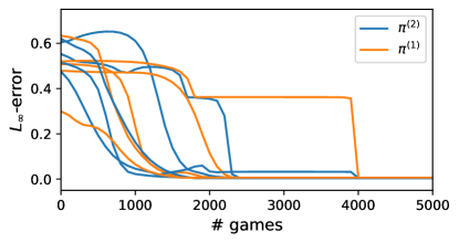
Figure 1: Training and convergence of 5 agents with random initialisation. Convergence of the 1-step and 2-step policies towards the optimal policies, measured by the $L_{\infty}$-norm.

4.2 Control problems

In this section we present a summary of the performance of the MPG algorithm on two standard RL problems, comparing its performance to a vanilla PG (VPG) algorithm [38] using deep neural networks to parametrise the preference function. Details and extended results can be found in F.2.

Frozen Lake:

The Frozen Lake benchmark [9] features a $k\times k$ grid composed of cells, holes and one treasure, and a discrete action space, namely, the agent can move in four directions (up, down, left, right). The game terminates when the agent reaches the treasure or falls down holes. In figure 2 (left), we show the number of victories during training for both methods for the $4\times 4$ grid. We observe a quicker learning from the MPG, with both methods finding the optimal policies at the end of training. The learning speed is quite sensitive to the choice of hyperparameters, so we deem the behaviour of both methods to be similar. Once the agents have been trained, we play 100 games and observe 90.60% of task completion, with an average path of 6.49 steps for the VPG, and 100% of task completion with an average path of length 6 (optimal path length) for the MPG.

Cart Pole:

The Cart Pole benchmark is a classical control problem. A pole is attached by an un-actuated joint to a cart, which moves along a frictionless track. The pole is placed upright on the cart, and the goal is to balance the pole by moving the cart to the left or right for some finite horizon time. It features a continuous environment and a discrete action space. The task is to balance the pole for 100 consecutive timesteps. In figure 2 (right), we show the cumulative reward during training per game. Once the agents have been trained, we again test them by playing 100 games. We attained successful task completion for 97.4% of the games, with an average of 99.76 consecutive timesteps for the MPG and successful task completion 97.2% of the games, with an average of 99.33 consecutive timesteps for the VPG. We observe similar performance between the MPG and the VPG during training and testing phases when the right set of hyperparameters is chosen.

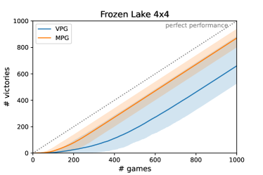
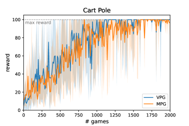
Figure 2: Performance of 5 agents during training. The solid curve represents the average and the shaded region the maximum and minimum observed at each game.

5 Conclusion

In this paper, we have studied a framework combining fixed-horizon RL and max-entropy RL. We have introduced the Matryoshka Policy Gradient algorithm in the function approximation setting, with log-linear parametric policies. We proved that the global optimum of the MPG objective is unique, and that MPG converges to this global optimum, including for continuous state and action space. Furthermore, we proved that these results hold true even when the true optimal policy does not belong to the parametric space (that is when Assumption A1. does not hold). The limit – globally optimal within the parametric space – corresponds to the orthogonal projection of the optimal policy onto the parametric space. It is written as the softmax of orthogonal projections of the optimal preferences onto the RKHSs of the parametrization, see (11). Finally, letting the horizon tend to infinity, the optimal policy of MPG retrieves the optimal policy of the standard infinite-horizon max-entropy objective. For neural policies, we prove that the limit is optimal within the RKHSs of the NTK (equivalently of the CK) at the end of training, and can be written in terms of orthogonal projections of optimal preferences onto these RKHSs, yielding criterion for global optimality in terms of the NTK (equivalently the CK). In particular it establishes the global convergence of neural MPG in the NTK regime. The MPG framework is intuitive, theoretically sound and it is easy to implement without standard RL tricks, as we verified in numerical experiments.

Limitations.

The main limitations of our work are the following: (a) we have not studied the rate of convergence of MPG (typically more assumptions on the environment, the horizon, are needed), (b) we assumed that the updates were perfect whereas in practice, one uses the estimate (3.2), (c) as a theoretical paper, our numerical experiments are rather simple. We hope to address these limitations in future work, as well a other perspectives such as:

• Additionally to MPG as defined in this paper, we expect to have nice theoretical properties of variations of MPG that are used for other PG algorithms. E.g. one can think of natural MPG, actor-critic MPG, path consistency MPG (see [32] for path consistency learning).

• We motivated the use of MPG with neural softmax policies by some theoretical, practical, and heuristic arguments; we believe that more can be said on the use of neural policies with MPG, in particular by studying the spectra of the NTK and the CK of neural networks along specific geodesics in the parametric space.

• How does the MPG framework compares to the standard max-entropy RL framework in terms of exploration, adversarial robustness, …?

Appendix

The appendix is organized as follows:

• A: we recall basic properties of softmax policies, then discuss the potential benefits to using a single neural network for the preferences of all $i$-step policies. This section ends with an explanation on how to approximate a kernel with finitely many features.

• B: we state and derive some basic facts on RKHS.

• C: We use concepts from Information Geometry to show that critical points of the MPG objective correspond to critical points of a Bregman divergence; this fact is useful when the realizable assumption does not hold to ensure that MPG converges to the unique global optimum.

• D: we prove the Matryoshka Policy Gradient Theorem (Theorem 1), Proposition 2 that shows that the infinite horizon optimal policy can approximated arbitrarily well by finite horizon optimal policies, Theorem 2 and Theorem 3 that shows global convergence of MPG.

• E: we list and discuss our main assumptions.

• F: we provide more detailed numerical experiments implementing MPG.

Appendix A More on the parametrization

A.1 Softmax policy

Softmax policies enjoy the two following properties:

• For all $s\in\mathcal{S}$, it holds that

  $$\mathbb{E}_{\pi_{\theta}}\left[\nabla_{\theta}\log\pi_{\theta}(A|s)\right]=\int_{\mathcal{A}}\nabla_{\theta}\pi_{\theta}(\mathrm{d}a|s)=0.$$ (12)

• As long as preferences are finite, it holds that $\pi_{\theta}(a|s)>0$ for all $(a,s)\in\mathcal{A}\times\mathcal{S}$.

In order to compute the learning rate’s value below which training converge, we use the following:

Lemma 2.

For the softmax policy with linear preferences, it holds that $\theta\mapsto\nabla_{\theta}J_{n}(\pi_{\theta})$ is $L$-Lipschitz for some $L>0$.

We refer to [44] Lemma 3.2 and the discussion after Assumption 3.1 therein for the proof of this fact in the standard setting; the proof straightforwardly adapts to the non-stationary policy setting.

A direct consequence of Lemma 2 is that gradient ascent on $J_{n}(\pi_{\theta})$ converges as soon as the learning rate is smaller than $1/L$.

A.2 Neural networks

Neural Tangent Kernel.

For a measurable nonlinearity $\sigma:\mathbb{R}\to\mathbb{R}$, we recursively define a neural network of depth $L\geq 1$, with trainable parameters $W^{\ell}\in\mathbb{R}^{d_{\ell}}\times\mathbb{R}^{d_{\ell+1}}$ as $f:x\in\mathbb{R}^{d_{0}}\mapsto\widetilde{\alpha}^{L}(x)\in\mathbb{R}^{d_{L}}$, with $\alpha^{0}(x):=x$ and

$$\widetilde{\alpha}^{\ell+1}(x) \ :=W^{\ell}\alpha^{\ell}(x),$$

$$\alpha^{\ell+1}(x) \ :=\sigma\left(\widetilde{\alpha}^{\ell+1}(x)\right),$$

where $\sigma$ is applied element-wise.

Note that the connection between the last hidden layer and the output layer is linear, since $f=W^{L}\alpha^{L-1}$. In particular, $f$ belongs to the RKHS of the conjugate kernel (CK) associated with the neural network, defined as

$$\Sigma(x,x^{\prime}):=\alpha^{L-1}(x)\cdot\alpha^{L-1}(x^{\prime}).$$

On the other hand, the training of the neural network is governed by the neural tangent kernel (NTK), which is defined as

$$\Theta(x,x^{\prime}):=\nabla f(x)\cdot\nabla f(x^{\prime})=\sum_{p=1}^{P}\partial_{\theta_{p}}f(x)\partial_{\theta_{p}}f(x^{\prime}),$$

where $\theta\in\mathbb{R}^{P}$ is the vector of all the trainable parameters of the neural network. It is important to note that both the CK and the NTK depend on the parameters and as such, move during training. Moreover, isolating the derivatives with respect to parameters $W^{L}$ of the last linear layer from the others $\widetilde{\theta}$, we have that

$$\Theta(x,x^{\prime}) =\alpha^{L-1}(x)\alpha^{L-1}(x^{\prime})+\nabla_{\widetilde{\theta}}f(x)\nabla_{\widetilde{\theta}}f(x^{\prime})$$

$$=\Sigma(x,x^{\prime})+K(x,x^{\prime}),$$

and $K$ is another positive semidefinite kernel. We therefore have that

$$\mathcal{H}_{\Sigma}\subset\mathcal{H}_{\Theta},\qquad\forall\theta\in\mathbb{R}^{P}.$$ (13)

Remark 1.

For infinitely wide neural networks in the NTK regime [24] (a.k.a. lazy regime [12], kernel regime), the NTK is fixed during training and is strictly positive definite, therefore convergence to the optimal policy is guaranteed.

Non-stationary policy parametrized by a single neural network.

One of the assumptions of MPG is that for any $i\neq j$, the policies $\pi^{(i)}_{\theta^{(i)}}$ and $\pi^{(j)}_{\theta^{(j)}}$ do not share parameters. Using one neural network per horizon becomes quickly costly as the maximal horizon increases. In order to avoid this issue, one can use a single neural network $h_{\theta}$ to parametrize all $i$-step policies by using $i$ as an input such that $\pi^{(i)}_{\theta}(a|s)\propto\overline{\pi}(a|s)\exp(h_{\theta}(a,s,i)/\tau)$. By deviating from the theory, we nonetheless expect the performance of the model to be enhanced: as $i$ grows large, the $i$-step optimal policy gets closer to the $i+1$-step policy. One could also use $1-\frac{1}{i}$ as an input to the network (or any increasing map $g:\mathbb{N}\mapsto\mathopen{[}0\,,1\mathclose{]}$ such that $i\mapsto g(i+1)-g(i)$ is decreasing).

A.3 Kernel methods

Suppose that $\Theta$ is a strictly pd kernel with $P$ positive eigenvalues. Recall the linear model $a\mapsto h_{\theta}(a)=\theta\cdot\psi(a)$, with parameters $\theta\in\mathbb{R}^{P}$, such that $\psi$ is a feature map associated with $\Theta$. Then if $P=\infty$, one can use random features, i.e. sample $g_{1},\ldots,g_{P^{\prime}}$ i.i.d. Gaussian processes with covariance kernel $\Theta$, then $h_{\theta}:=\frac{1}{\sqrt{P^{\prime}}}\sum_{i=1}^{P^{\prime}}\theta_{i}g_{i}$. One can thus approximate the true kernel predictor using a finite number of features, see [25].

Another way to approximate the kernel predictor with finitely many features is to use the spectral truncated kernel $\widehat{\Theta}$ of rank $P^{\prime}\in\mathbb{N}$, by cutting off the smallest eigenvalues. If $(e_{i},\lambda_{i})_{i\geq 1}$ are the eigenfunction/eigenvalue pairs of $\Theta$ ranked in the non-increasing order of $\lambda_{i}$, one can use

$$\widehat{\Theta}(x,x^{\prime}):=\sum_{i=1}^{P^{\prime}}\lambda_{i}e_{i}(x)e_{i}(x^{\prime}),$$

and the predictor $h_{\theta}:=\sum_{i=1}^{P^{\prime}}\theta_{i}e_{i}$.

Appendix B Reproducible kernel Hilbert spaces

In this section, we recall and provide some basic facts on RKHSs that we use throughout the proofs. Given some RKHS $\mathcal{H}$, we write $\mathcal{H}^{\perp}$ for its orthogonal complement; it is also an RKHS.

Lemma 3.

Let $\mathcal{H}_{1},\mathcal{H}_{2}$ be two RKHSs on $\mathcal{A}\times\mathcal{S}$,

1. The intersection $\mathcal{H}_{1}\cap\mathcal{H}_{2}$ is an RKHS.

2. For any element $f\in\mathcal{H}_{1}$, there exists a unique decomposition $f=g_{\bullet}+g_{\perp}$ such that $g_{\bullet}\in\mathcal{H}_{1}\cap\mathcal{H}_{2}$ and $g_{\perp}\in\mathcal{H}_{1}\cap(\mathcal{H}_{2})^{\perp}$.

For a probability measure of the form $\mu(\mathrm{d}s)\pi(\mathrm{d}a|s)$ on $\mathcal{A}\times\mathcal{S}$, where $\pi$ is a policy, and for a positive-semidefinite kernel $K$ on $\mathcal{A}\times\mathcal{S}$, we define the integral operator $I_{K}(\mu,\pi):L^{2}(\mu(\mathrm{d}s)\pi(\mathrm{d}a|s))$ by

$$I_{K}(f;\mu,\pi):(a,s)\mapsto\int_{\mathcal{A}\times\mathcal{S}}\mu(\mathrm{d}s^{\prime})\pi(\mathrm{d}a^{\prime}|s^{\prime})f(a^{\prime},s^{\prime})K((a,s),(a^{\prime},s^{\prime})).$$

Mercer’s Theorem states that if $\mathcal{A}\times\mathcal{S}$ is closed (in a real space), $\mu(\mathrm{d}s)\pi(\mathrm{d}a|s)$ has full support, and if $K$ is continuous and satisfies $\int_{(\mathcal{A}\times\mathcal{S})^{2}}K((a,s),(a^{\prime},s^{\prime}))^{2}<\infty$, then there exists eigenfunction/eigenvalue pairs $(e_{i},\lambda_{i})_{i\geq 1}$ associated with $I_{K}(\mu,\pi)$, ranked in the non-increasing order of $\lambda_{i}\geq 0$ such that

$$K((a,s),(a^{\prime},s^{\prime}))=\sum_{i\geq 1}\lambda_{i}e_{i}(a,s)e_{i}(a^{\prime},s^{\prime}).$$

Moreover, $\{e_{i};i\geq 1\}$ is an orthonormal basis of $L^{2}(\mu(\mathrm{d}s)\pi(\mathrm{d}a|s))$ and the RKHS $\mathcal{H}_{K}$ has orthonormal basis $\{\sqrt{\lambda_{i}}e_{i};\lambda_{i}>0\}$ with respect to the RKHS inner product. We refer the reader to [31] for more details.

We stress that the notion of orthogonality depends on the measure $\mu(\mathrm{d}s)\pi(\mathrm{d}a|s)$. Henceforth, we write $\mathcal{H}^{\perp}$ for the orthogonal space of the RKHS, where this measure is implicit but given by the context.

In the rest of the current section, we use the notation introduced above and assume that Mercer’s Theorem applies.

Lemma 4.

Let $f\in L^{2}(\mu(\mathrm{d}s)\pi(\mathrm{d}a|s))$. It holds that $I_{K}(f;\mu,\pi)(a,s)=0$ for all $a\in\mathcal{A},s\in\mathcal{S}$ if and only if $f\in(\mathcal{H}_{K})^{\perp}$.

Proof.

We write

$$\int_{\mathcal{A}\times\mathcal{S}}\mu(\mathrm{d}s)\pi(\mathrm{d}a|s)f(a,s)I_{K}(f;\mu,\pi)(a,s)$$

$$\hskip 28.45274pt=\int_{(\mathcal{A}\times\mathcal{S})^{2}}\mu(\mathrm{d}s)\pi(\mathrm{d}a|s)(a,s)\int_{\mathcal{A}\times\mathcal{S}}\mu(\mathrm{d}s^{\prime})\pi(\mathrm{d}a^{\prime}|s^{\prime})f(a,s)f(a^{\prime},s^{\prime})K((a,s),(a^{\prime},s^{\prime}))$$

$$\hskip 28.45274pt=\sum_{i\geq 1}\lambda_{i}\left(\int_{\mathcal{A}\times\mathcal{S}}\mu(\mathrm{d}s)\pi(\mathrm{d}a|s)f(a,s)e_{i}(a,s)\right)^{2},$$

where we used Mercer’s Theorem to write $K((a,s),(a^{\prime},s^{\prime}))=\sum_{i\geq 1}\lambda_{i}e_{i}(a,s)e_{i}(a^{\prime},s^{\prime})$. The claim follows. ∎

Lemma 5.

It holds that

$$\widetilde{K}((a,s),(a^{\prime},s^{\prime})):=\ K((a,s),(a^{\prime},s^{\prime}))-\int_{\mathcal{A}}K((b,s),(a^{\prime},s^{\prime}))\pi(\mathrm{d}b|s)$$

$$\hskip 19.91684pt-\int_{\mathcal{A}}K((a,s),(b^{\prime},s^{\prime}))\pi(\mathrm{d}b^{\prime}|s^{\prime})+\int_{\mathcal{A}^{2}}K((b,s),(b^{\prime},s^{\prime}))\pi(\mathrm{d}b|s)\pi(\mathrm{d}b^{\prime}|s^{\prime})$$

is a positive-semidefinite kernel. Furthermore, any map $g\in\mathcal{H}_{K}\cap(\mathcal{H}_{\widetilde{K}})^{\perp}$ is such that for every $s\in\mathcal{S}$, the map $a\mapsto g(a,s)$ is constant.

Proof.

Let $d:=\sup\{i\geq 1:\lambda_{i}>0\}$ where the $\lambda_{i}$’s are the eigenvalues of $I_{K}$. To prove the first part of the claim, it suffices to show that for all $g\in L^{2}(\mu(\mathrm{d}s)\pi(\mathrm{d}a|s))$, we have

$$\int_{(\mathcal{S}\times\mathcal{A})^{2}}\mu(\mathrm{d}s)\pi(\mathrm{d}a|s)\mu(\mathrm{d}s^{\prime})\pi(\mathrm{d}a^{\prime}|s^{\prime})g(a,s)g(a^{\prime},s^{\prime})\widetilde{K}((a,s),(a^{\prime},s^{\prime}))\geq 0.$$ (14)

To ease the notation, for any maps $f,g\in L^{2}(\mu(\mathrm{d}s)\pi(\mathrm{d}a|s))$ we write

$$\langle f,g\rangle:=\ \int_{\mathcal{S}\times\mathcal{A}}\mu(\mathrm{d}s)\pi(\mathrm{d}a|s)f(a,s)g(a,s),$$

$$\overline{f}(s):=\ \int_{\mathcal{A}}\pi(\mathrm{d}a|s)f(a,s).$$

We now establish (14). Using that $K((a,s),(a^{\prime},s^{\prime}))=\sum_{j\leq d}\lambda_{j}e_{j}(a,s)e_{j}(a^{\prime},s^{\prime})$, we get

$$\widetilde{K}((a,s),(a^{\prime},s^{\prime}))=\sum_{j\leq d}\lambda_{j}(e_{j}(a,s)-\overline{e}_{j}(s))(e_{j}(a^{\prime},s^{\prime})-\overline{e}_{j}(s^{\prime})).$$

The left-hand side of (14) thus reads as

$$\sum_{j\leq d}\lambda_{j}\left(\langle g,e_{j}\rangle^{2}-2\langle g,e_{j}\rangle\langle\overline{g},\overline{e}_{j}\rangle+\langle\overline{g},\overline{e}_{j}\rangle^{2}\right) =\sum_{j\leq d}\lambda_{j}\left(\alpha_{j}^{2}-2\alpha_{j}\langle\overline{g},\overline{e}_{j}\rangle+\langle\overline{g},\overline{e}_{j}\rangle^{2}\right)$$

$$=\sum_{j\leq d}\lambda_{j}\left(\alpha_{j}-\langle\overline{g},\overline{e}_{j}\rangle\right)^{2}.$$

The right-hand side above being clearly non-negative, this shows that $\widetilde{K}$ is positive-semidefinite.

We now turn our attention to the last part of the claim. Suppose that $g\in\mathcal{H}_{K}\cap(\mathcal{H}_{\widetilde{K}})^{\perp}$, so that we can write $g=\sum_{j\leq d}\alpha_{j}e_{j}$, with $\alpha_{j}=\langle g,e_{j}\rangle$. Moreover, by Lemma 4, we have an equality in (14), and we get

$$\sum_{j\leq d}\lambda_{j}(\langle g,e_{j}\rangle-\langle\overline{g},\overline{e}_{j}\rangle)^{2}=0.$$

We thus necessarily have $\langle g,e_{j}\rangle=\langle\overline{g},\overline{e}_{j}\rangle$ for all $j\leq d$. In particular,

$$\langle g,g\rangle =\sum_{j\leq d}\alpha_{j}^{2}=\sum_{j\leq d}\alpha_{j}\langle\overline{g},\overline{e}_{j}\rangle=\langle\overline{g},\overline{g}\rangle.$$

On the other hand, Cauchy-Schwarz Inequality shows that if $s\mapsto g(a,s)$ is not constant in $a$ for all $s$, then

$$\langle g,g\rangle =\int_{\mathcal{S}}\mu(\mathrm{d}s)\int_{\mathcal{A}}\pi(\mathrm{d}a|s)g(a,s)^{2}$$

$$>\int_{\mathcal{S}}\mu(\mathrm{d}s)\left(\int_{\mathcal{A}}\pi(\mathrm{d}a|s)|g(a,s)|\right)^{2}$$

$$\geq\langle\overline{g},\overline{g}\rangle.$$

This is a contradiction and thus implies that $g$ must be constant in $a$. ∎

Appendix C Information Geometry

The goal of this section is to show that a Pythagorean identity that is used in the forthcoming proof of Theorem 3. We use it in the case of a $1$-step policy, and for a fixed state distribution with full support, that we denote by $\nu$ in this section. Without loss of generality, we also assume to ease the notation that $\tau=1$.

Consider the parametric space of preferences $\mathcal{H}_{\Theta}:=\{h_{\theta}=\sum_{k=1}^{d}\theta_{k}\psi_{k};\theta\in\mathbb{R}^{d}\}$, where $\psi$ is the feature map of a positive definite kernel $\Theta$ that we assume to be continuous and bounded. The space $\mathcal{H}_{\Theta}$ is the RKHS associated with $\Theta$. Fix $\vartheta\in\mathbb{R}^{d}$ and let $\pi_{\vartheta}$ be the $1$-step policy induced by the preference $h_{\vartheta}$ (with baseline policy $\overline{\pi}$ as usual).

Let $\varphi_{k}=\psi_{k}$ if $k\leq d$, and otherwise define $\varphi_{k}$ such that $\{\varphi_{k};k\geq d+1\}$ is an orthonormal basis of $(\mathcal{H}_{\Theta})^{\perp}$, the orthogonal complement of $\mathcal{H}_{\Theta}$ in $L^{2}(\nu(\mathrm{d}s)\pi_{\vartheta}(\mathrm{d}a|s))$. For any $d^{\prime}$, let $\mathcal{F}_{d^{\prime}}:=\{h=\sum_{k=1}^{d^{\prime}}\theta_{k}\varphi_{k}\}$. We denote by $\mathscr{P}(d^{\prime})$ the set of policies whose preferences belong to $\mathcal{F}_{d^{\prime}}$.

The map

$$F:\theta \mapsto\int_{\mathcal{S}}\nu(\mathrm{d}s)\log\int_{\mathcal{A}}\overline{\pi}(\mathrm{d}a|s)e^{h_{\theta}(a,s)}$$

$$\mathbb{R}^{d^{\prime}} \to\mathbb{R}$$

is strictly convex on $\mathscr{P}(d)$. Indeed, it is straightforward to compute

$$\partial_{\theta_{i}}F(\theta) =\int_{\mathcal{S}}\nu(\mathrm{d}s)\int_{\mathcal{A}}\pi_{\theta}(\mathrm{d}a|s)\varphi_{i}(a,s),$$

and then

$$\nabla_{\theta}\nabla_{\theta}F(\theta) =\left(\int_{\mathcal{S}}\nu(\mathrm{d}s)\int_{\mathcal{A}}\pi_{\theta}(\mathrm{d}a|s)\varphi_{j}(a,s)(\varphi_{j}(a,s)-\mathbb{E}_{\pi_{\theta}}[\varphi_{j}(A,s)])\right)_{i,j\leq d^{\prime}}$$

$$=\int_{\mathcal{S}}\nu(\mathrm{d}s)\mathrm{Var}_{\pi_{\theta}}\left[\varphi(A,s)\right],$$

where $\mathrm{Var}_{\pi_{\theta}}\left[\varphi(A,s)\right]$ is the covariance matrix of $\varphi(A,s)$ for $A\sim\pi_{\theta}(\cdot|s)$. In particular, it is positive definite for all $s$, which implies that $\nabla_{\theta}\nabla_{\theta}F$ is positive definite, and then that $F$ is strictly convex.

As a strictly convex map, $F$ induces a Bregman divergence on $\mathscr{P}(d^{\prime})$, given in terms of the coordinate system $\theta\in\mathbb{R}^{d^{\prime}}$ by

$$D_{F}(\theta,\theta^{\prime}): =F(\theta)-F(\theta^{\prime})-\nabla F(\theta^{\prime})\cdot(\theta-\theta^{\prime})$$

$$=\int_{\mathcal{S}}\nu(\mathrm{d}s)D_{\mathrm{KL}}(\pi_{\theta^{\prime}}||\pi_{\theta})(s).$$

More generally, $D_{F}(\pi,\pi^{\prime}):=\int_{\mathcal{S}}\nu(\mathrm{d}s)D_{\mathrm{KL}}(\pi^{\prime}||\pi)(s)$ is well defined for any policies $\pi,\pi^{\prime}\in\mathcal{P}$. One can define a dual coordinate system $\xi(\theta):=\nabla F(\theta)$, and the manifold $\mathscr{P}(d^{\prime})$ is said to be dually flat, as each coordinate system induces a notion of flatness.

Recall that $\vartheta\in\mathbb{R}^{d}$ is fixed and let $\widehat{Q}\in L^{2}(\nu(\mathrm{d}s)\pi_{\vartheta}(\mathrm{d}a|s))$, with $\widehat{\pi}$ the induced policy. In particular, we can write $\widehat{Q}=\sum_{k=1}^{\infty}\widehat{\theta}_{k}\varphi_{k}$. For all $d^{\prime}\geq 1$, let $\widehat{\pi}_{d^{\prime}}\in\mathscr{P}(d^{\prime})$ be the policy induced by $\widehat{h}_{d^{\prime}}:=\sum_{k=1}^{d^{\prime}}\widehat{\theta}_{k}\varphi_{k}\in\mathcal{F}_{d^{\prime}}$. Note that $\mathscr{P}(d)$ is a flat submanifold of $\mathscr{P}(d^{\prime})$. In particular, by Theorem 1.5 in [3] p.27, we have that

$$\widehat{\pi}_{d}^{d^{\prime}}:=\mathrm{argmin}_{\pi_{\theta}\in\mathscr{P}(d)}D_{F}(\widehat{\pi}_{d^{\prime}},\pi_{\theta})$$

is unique, and moreover,

$$D_{F}(\widehat{\pi}_{d^{\prime}},\pi_{\vartheta})=D_{F}(\widehat{\pi}_{d^{\prime}},\widehat{\pi}_{d}^{d^{\prime}})+D_{F}(\widehat{\pi}_{d}^{d^{\prime}},\pi_{\vartheta}).$$

We now extend this identity to the infinite dimensional case, that is, with $\widehat{\pi}$ in place of $\widehat{\pi}_{d^{\prime}}$.

Firstly, it is clear that $\widehat{\pi}_{d^{\prime}}\to\widehat{\pi}$ as $d^{\prime}\to\infty$. Since $D_{F}$ is continuous, the Maximum Theorem (see p.116 of [5]) entails that

$$\pi^{\infty}_{d}:=\lim_{d^{\prime}\to\infty}\widehat{\pi}^{d^{\prime}}_{d}=\mathrm{argmin}_{\pi_{\theta}\in\mathscr{P}(d)}D_{F}(\widehat{\pi},\pi_{\theta}),$$

and then

$$D_{F}(\widehat{\pi},\pi_{\vartheta})=D_{F}(\widehat{\pi},\widehat{\pi}_{d}^{\infty})+D_{F}(\widehat{\pi}_{d}^{\infty},\pi_{\vartheta}).$$

(Alternatively, one can show the above as Equation (4) in [18])

From the above equation we easily deduce the following Lemma:

Lemma 6.

With the notation introduced above, the vector $\vartheta\in\mathbb{R}^{d}$ is a critical point of $\theta\mapsto D_{F}(\widehat{\pi},\pi_{\theta})$ if and only if it is a critical point of $\theta\mapsto D_{F}(\widehat{\pi}_{d}^{\infty},\pi_{\theta})$.

Appendix D Proofs

D.1 Matryoshka Policy Gradient Theorem

Proof of Theorem 1.

Let $\mathbf{m}_{\pi}^{(i)}$ denote the law of $S_{n-i}$, that is, the $(n-i)$-th visited state under $\pi$. The distribution of the sequence $S_{0},A_{0},\ldots,A_{n-i-1},S_{n-i}$ is not influenced by the parameters $\theta^{(i)}$, thus we can write

$$\nabla_{\theta^{(i)}}J_{n}(\pi_{t}) =\int_{\mathcal{S}}\nabla_{\theta^{(i)}}V_{\pi_{t}}^{(n)}(s)\nu_{0}(\mathrm{d}s)$$

$$=\nabla_{\theta^{(i)}}\bigg{(}\mathbb{E}_{\pi_{t}}\bigg{[}\sum_{\ell=0}^{n-i-1}R_{\ell}-\tau\log\frac{\pi_{t}^{(n-\ell)}}{\overline{\pi}}(A_{\ell}|S_{\ell})\bigg{]}$$

$$\hskip 56.9055pt+\mathbb{E}_{S_{n-i}\sim\mathbf{m}_{\pi_{t}}^{(i)}}\bigg{[}\mathbb{E}_{\pi_{t}}\bigg{[}\sum_{\ell=n-i}^{n}R_{\ell}-\tau\log\frac{\pi_{t}^{(n-\ell)}}{\overline{\pi}}(A_{\ell}|S_{\ell})\Big{|}S_{n-i}\bigg{]}\bigg{]}\bigg{)}$$

$$=0+\mathbb{E}_{S_{n-i}\sim\mathbf{m}_{\pi_{t}}^{(i)}}\bigg{[}\nabla_{\theta^{(i)}}V_{\pi_{t}}^{(i)}(S_{n-i})\bigg{]},$$

where we have used the Markov property. We then have that

$$\nabla_{\theta^{(i)}}V_{\pi_{t}}^{(i)}(S_{n-i}) =\nabla_{\theta^{(i)}}\mathbb{E}_{T_{n,i}(\pi_{t})}\bigg{[}\sum_{\ell=n-i}^{n}R_{\ell}-\tau\log\frac{\pi^{(n-\ell)}_{t}}{\overline{\pi}}(A_{\ell}|S_{\ell})\bigg{|}S_{n-i}\bigg{]}$$

$$=\mathbb{E}_{T_{n,i}(\pi_{t})}\bigg{[}\bigg{(}\sum_{\ell=n-i}^{n}\bigg{(}R_{\ell}-\tau\log\frac{\pi^{(n-\ell)}_{t}}{\overline{\pi}}(A_{\ell}|S_{\ell})\bigg{)}-\tau\bigg{)}\nabla\log\pi_{t}^{(i)}(A_{n-i}|S_{n-i})\Big{|}S_{n-i}\bigg{]}$$

$$=\mathbb{E}_{T_{n,i}(\pi_{t})}\bigg{[}\sum_{\ell=n-i}^{n}\bigg{(}R_{\ell}-\tau\log\frac{\pi^{(n-\ell)}_{t}}{\overline{\pi}}(A_{\ell}|S_{\ell})\bigg{)}\nabla\log\pi_{t}^{(i)}(A_{n-i}|S_{n-i})\Big{|}S_{n-i}\bigg{]},$$

where we have used (12) to get rid of $\tau$.

Recalling the MPG update (3.2), we thus have proved that $\mathbb{E}[\theta_{t+1}-\theta_{t}]=\eta\nabla_{\theta}J_{n}(\pi_{t})$; the convergence follows from Lemma 2. ∎

D.2 On the optimal policy

Proof of Lemma 1.

By definition, we write

$$V_{*}^{(n)}(s) =\tau\int_{\mathcal{A}}\pi_{*}^{(n)}(\mathrm{d}a|s)\left(Q_{*}^{(n)}(a,s)-\tau\log\frac{\pi_{*}^{(n)}}{\overline{\pi}}(a|s)\right)$$

$$=\tau\log\mathbb{E}_{\overline{\pi}}\left[\exp(Q_{*}^{(n)}(A,s)/\tau)\right]\int_{\mathcal{A}}\overline{\pi}(\mathrm{d}a|s)\frac{\exp\left(Q_{*}^{(n)}(a,s)/\tau\right)}{\mathbb{E}_{\overline{\pi}}\left[\exp\left(Q_{*}^{(n)}(A,s)/\tau\right)\right]}$$

$$=\tau\log\mathbb{E}_{\overline{\pi}}\left[\exp\left(Q_{*}^{(n)}(A,s)/\tau\right)\right],$$

as claimed, which concludes the proof. ∎

Proof of Proposition 2.

(i) Let $\pi\in\mathcal{P}$ be any standard policy, and let $\pi_{n}=(\pi,\ldots,\pi)\in\mathcal{P}_{n}$. By definition of the standard infinite-horizon discounted objective $J_{\infty}$, using the dominated convergence theorem (rewards are bounded), we have that $J_{n}(\pi_{n})\to J_{\infty}(\pi)$. In particular, we get that $\pi_{*,n}^{(n)}$ achieves a performance arbitrarily close to that of $\pi_{*,\infty}$ in the infinite horizon discounted setting, and since the optimal policy of $J_{\infty}$ is unique (Lebesgue almost everywhere), we deduce that $\pi_{*,n}^{(n)}\to\pi_{*,\infty}$ as $n\to\infty$.

(ii) Suppose that $J_{1}(\pi_{*,1})>J_{1}(T_{n,1}(\pi_{*,n}))$, that is

$$\int_{\mathcal{S}}V_{\pi_{*,1}}^{(1)}(s)\nu_{0}(\mathrm{d}s)>\int_{\mathcal{S}}V_{\pi_{*,n}}^{(1)}(s)\nu_{0}(\mathrm{d}s).$$

In particular, the set $\widetilde{\mathcal{S}}\subset\mathcal{S}$ such that $s\in\widetilde{\mathcal{S}}$ if and only if $V_{\pi_{*,1}}^{(1)}(s)>V_{\pi_{*,n}}^{(1)}(s)$ is non-empty and has a positive Lebesgue measure. Furthermore, by optimality, $s\in\mathcal{S}\setminus\widetilde{\mathcal{S}}$ if and only if $V_{\pi_{*,1}}^{(1)}(s)=V_{\pi_{*,n}}^{(1)}(s)$. Let $\widetilde{\pi}_{*,n}\in\mathcal{P}_{n}$ be identical to $\pi_{*,n}$ except for the 1-step policy where $\pi_{*,n}^{(1)}$ is replaced by $\pi_{*,1}$. Then, the recursive structure of the value function (1) entails that $J_{n}(\widetilde{\pi}_{*,n})>J_{n}(\pi_{*,n})$ (we implicitly use that the MDP preserves the absolute continuity of its state’s law), which is a contradiction. Therefore, $T_{n,1}(\pi_{*,n})=\pi_{*,1}$.

Then, by induction and using the recursive structure of the value function, the same argument shows that $T_{n,m}(\pi_{*,n})=\pi_{*,m}$ for all $m=2,\ldots,n-1$, which concludes the proof. ∎

D.3 Global optimality of MPG: realizable case

Lemma 7.

For all $n\geq 1$, all $\pi\in\mathcal{P}_{n}$ and all $s\in\mathcal{S}$, it holds that

$$V_{\pi}^{(n)}(s)-V_{*}^{(n)}(s)=-\mathbb{E}_{\pi}\left[\left.\sum_{i=0}^{n-1}D_{\mathrm{KL}}(\pi^{(n-i)}||\pi_{*}^{(n-i)})(S_{i})\right|S_{0}=s\right].$$

Proof.

Recall (1) and write

$$V_{\pi}^{(n)}(s) =\int_{\mathcal{A}}\pi^{(n)}(\mathrm{d}a|s)\bigg{(}r(a,s)-\tau\log\frac{\pi^{(n)}}{\overline{\pi}}(a|s)+\int_{\mathcal{S}}p(s,a,\mathrm{d}s^{\prime})V^{(n-1)}_{\pi}(s^{\prime})\bigg{)}$$

$$=\int_{\mathcal{A}}\pi^{(n)}(\mathrm{d}a|s)\bigg{(}V_{*}^{(n)}(s)-\tau\log\frac{\pi^{(n)}}{\pi_{*}}(a|s)+\int_{\mathcal{S}}p(s,a,\mathrm{d}s^{\prime})(V^{(n-1)}_{\pi}(s^{\prime})-V_{*}^{(n-1)}(s^{\prime}))\bigg{)},$$

where we plugged in the expression of the optimal policy (5). We can rewrite the above as

$$V_{\pi}^{(n)}(s)-V_{*}^{(n)}(s)=-D_{\mathrm{KL}}(\pi^{(n)}||\pi_{*}^{(n)})+\mathbb{E}\left[V^{(n-1)}_{\pi}(S_{1})-V_{*}^{(n-1)}(S_{1})\Big{|}S_{0}=s\right].$$

The claim follows by induction. ∎

Proof of Proposition 1.

The Kullback-Leibler divergence being non-negative, it is readily seen that for all $s\in\mathcal{S}$, the maximal value of $\pi\mapsto V_{\pi}^{(n)}(s)$ is obtained for $\pi=\pi_{*}$. It is then immediate that $\pi_{*}$ is the unique optimal policy (Lebesgue-almost everywhere) for the objective $J_{n}$ given in (4). ∎

Lemma 8.

Let $t\in\mathbb{N}$ and $m\in\{1,\ldots,n\}$. Suppose that $\pi_{t}^{(k)}=\pi_{*}^{(k)}$ for all $k=1,\ldots,m-1$. For all $a\in\mathcal{A}$ and $s\in\mathcal{S}$, it holds that

$$\log\pi^{(m)}_{t+1}(a|s)-\log\pi^{(m)}_{t}(a|s)$$

$$\hskip 28.45274pt=-\eta\tau\int_{\mathcal{S}}\mathbf{m}_{\pi_{t}}^{(m)}(\mathrm{d}s^{\prime})\int_{\mathcal{A}}\pi^{(m)}_{t}(\mathrm{d}a^{\prime}|s^{\prime})\left(\log\frac{\pi^{(m)}_{t}}{\pi^{(m)}_{*}}(a^{\prime}|s^{\prime})-D_{\mathrm{KL}}(\pi^{(m)}_{t}||\pi^{(m)}_{*})(s^{\prime})\right)$$

$$\hskip 85.35826pt\times\left(\Theta^{(m)}((a,s),(a^{\prime},s^{\prime}))-\mathbb{E}_{\pi^{(m)}_{t}}[\Theta^{(m)}((A,s),(a^{\prime},s^{\prime}))]\right)+o\left(\eta C(\theta_{t})\right),$$

where $\mathbf{m}_{\pi_{t}}^{(m)}$ is the law of $S_{n-m}$ under policy $\pi_{t}$ and the constant $C(\theta_{t})$ does not depend on $\eta$.

Proof.

The gradient of the policy reads as

$$\nabla_{\theta}\pi^{(m)}_{t}(a|s) =\frac{1}{\tau}\pi^{(m)}_{t}(a|s)\int_{\mathcal{A}}\left(\delta_{a,\mathrm{d}a^{\prime}}-\pi^{(m)}_{t}(\mathrm{d}a^{\prime}|s)\right)\nabla_{\theta}h^{(m)}_{t}(a,s).$$ (15)

Let $(a,s)\in\mathcal{A}\times\mathcal{S}$. Using (3.2) and a first order Taylor approximation, we write

$$\log\pi_{t+1}^{(m)}(a|s)-\log\pi_{t}^{(m)}(a|s) =(\theta_{t+1}^{(m)}-\theta_{t}^{(m)})\cdot\frac{\nabla_{\theta}\pi_{t}^{(m)}(a|s)}{\pi_{t}^{(m)}(a|s)}+o\left(\eta C(\theta_{t})\right)$$

$$=\frac{\eta}{\tau^{2}}\mathbb{E}_{\pi_{t}}\bigg{[}C_{m}\int_{\mathcal{A}\times\mathcal{A}}\left(\delta_{a,\mathrm{d}a^{\prime}}-\pi_{t}^{(m)}(\mathrm{d}a^{\prime}|s)\right)$$

$$\hskip 11.38092pt\times\left(\delta_{A_{n-m},\mathrm{d}a^{\prime\prime}}-\pi_{t}^{(m)}(\mathrm{d}a^{\prime\prime}|S_{n-m})\right)\Theta^{(m)}((a^{\prime},s),(a^{\prime\prime},S_{n-m}))\bigg{]}$$

$$\hskip 213.39566pt+o\left(\eta C(\theta_{t})\right).$$ (16)

We focus on the expectation. It is equal to

$$\mathbb{E}_{\pi_{t}}\bigg{[}C_{m}\bigg{(}\Theta^{(m)}((a,s),(A_{n-m},S_{n-m}))-\mathbb{E}_{A}\left[\Theta^{(m)}((A,s),(A_{n-m},S_{n-m}))\right]$$

$$\hskip 85.35826pt-\mathbb{E}_{A}\left[\Theta^{(m)}((a,s),(A^{\prime},S_{n-m}))\right]+\mathbb{E}_{A,A^{\prime}}\left[\Theta^{(m)}((A,s),(A^{\prime},S_{n-m}))\right]\bigg{)}\bigg{]},$$

where $A,A^{\prime}$ have respective laws $\pi_{t}^{(m)}(\cdot|s)$ and $\pi_{t}^{(m)}(\cdot|S_{n-m})$ and are mutually independent of all other variables (conditionally given $S_{n-m}$ for $A^{\prime}$). Using the trick $\mathbb{E}[X(Y-\mathbb{E}[Y])]=\mathbb{E}_{[}(X-\mathbb{E}[X])Y]$, we obtain

$$\mathbb{E}_{\pi_{t}}\Big{[}\left(C_{m}-\mathbb{E}\left[C_{m}|S_{n-m}\right]\right)\Big{(}\Theta^{(m)}((a,s),(A_{n-m},S_{n-m}))-\mathbb{E}_{A}\left[\Theta^{(m)}((A,s),(A_{n-m},S_{n-m}))\right]\Big{)}\Big{]}.$$ (17)

We write

$$\mathbb{E}\left[C_{m}|S_{n-m}\right] =\mathbb{E}\left[\sum_{\ell=n-m}^{n}\left(R_{\ell}-\tau\log\frac{\pi_{t}^{(n-\ell)}}{\overline{\pi}}(A_{\ell}|S_{\ell})\right)\bigg{|}S_{n-m}\right]$$

$$=V_{\pi_{t}}^{(m)}(S_{n-m})$$

$$=V_{*}^{(m)}(S_{n-m})-D_{\mathrm{KL}}(\pi_{t}^{(m)}||\pi_{*}^{(m)})(S_{n-m}),$$

where we used Lemma 7 and the fact that $\pi_{t}^{(i)}=\pi_{*}^{(i)}$ for all $i=1,\ldots,m-1$. Similarly and using the expression (5) of the optimal policy, we have

$$\mathbb{E}[C_{m}|S_{n-m},A_{n-m}] =R_{n-m}-\tau\log\frac{\pi_{t}^{(m)}}{\overline{\pi}}(A_{n-m}|S_{n-m})+\mathbb{E}\left[V_{\pi_{t}}^{(m-1)}(S_{n-m})\Big{|}S_{n-m},A_{n-m}\right]$$

$$=\mathbb{E}\Big{[}V_{\pi_{t}}^{(m-1)}(S_{n-m+1})-V_{*}^{(m-1)}(S_{n-m+1})\Big{|}S_{n-m},A_{n-m}\Big{]}$$

$$\hskip 113.81102pt-\tau\log\frac{\pi_{t}^{(m)}}{\pi_{*}^{(m)}}(A_{n-m}|S_{n-m})+V_{*}^{(m)}(S_{n-m})$$

$$=-\tau\log\frac{\pi_{t}^{(m)}}{\pi_{*}^{(m)}}(A_{n-m}|S_{n-m})+V_{*}^{(m)}(S_{n-m}).$$

Hence, the expression in (17) becomes

$$\tau\mathbb{E}_{\pi_{t}}\bigg{[}\bigg{(}D_{\mathrm{KL}}(\pi_{t}^{(m)}||\pi_{*}^{(m)})(A_{n-m}|S_{n-m})-\log\frac{\pi_{t}^{(m)}}{\pi_{*}^{(m)}}(A_{n-m}|S_{n-m})\bigg{)}\Big{(}\Theta^{(m)}((a,s),(A_{n-m},S_{n-m}))$$

$$\hskip 247.53888pt-\mathbb{E}_{A}\left[\Theta^{(m)}((A,s),(A_{n-m},S_{n-m}))\right]\Big{)}\bigg{]},$$

which corresponds to the first order term in right-hand side of the equation in the Lemma. Coming back to (D.3), this concludes the proof. ∎

Proof of Theorem 2.

We reason by induction. Let $m\leq n$, suppose that $\pi^{(i)}_{t}\equiv\pi^{(i)}_{*}$ for all $i=1,\ldots,m-1$, and that $\pi^{(i)}_{t}=\pi^{(i)}_{\infty}$ for all $i=m,\ldots,n$. In particular, we are at a critical point $(\theta^{(1)}_{t},\ldots,\theta^{(n)}_{t})$ of $(\theta^{(1)},\ldots,\theta^{(n)})\mapsto J_{n}(\pi_{\theta})$. Let $a\in\mathcal{A},s\in\mathcal{S}$. By Lemma 8, we have that

$$0 =\log\pi^{(m)}_{t+1}(a|s)-\log\pi^{(m)}_{t}(a|s)$$

$$=-\eta\tau\int_{\mathcal{A}\times\mathcal{S}}\mathbf{m}_{\pi_{t}}^{(m)}(\mathrm{d}s^{\prime})\pi_{t}^{(m)}(\mathrm{d}a^{\prime}|s^{\prime})\left(\log\frac{\pi_{t}^{(m)}}{\pi_{*}^{(m)}}(a^{\prime}|s^{\prime})-D_{\mathrm{KL}}(\pi_{t}^{(m)}||\pi_{*}^{(m)})(s^{\prime})\right)$$

$$\hskip 85.35826pt\times\bigg{(}\Theta^{(m)}((a,s),(a^{\prime},s^{\prime}))-\mathbb{E}_{\pi^{(m)}_{t}}[\Theta^{(m)}((A,s),(a^{\prime},s^{\prime}))]\bigg{)}+o\left(\eta C(\theta_{t})\right),$$

Since the above must be true for all $\eta>0$, we deduce that

$$\int_{\mathcal{A}\times\mathcal{S}}\mathbf{m}_{\pi_{t}}^{(m)}(\mathrm{d}s^{\prime})\pi_{t}^{(m)}(\mathrm{d}a^{\prime}|s^{\prime})\left(\log\frac{\pi_{t}^{(m)}}{\pi_{*}^{(m)}}(a^{\prime}|s^{\prime})-D_{\mathrm{KL}}(\pi_{t}^{(m)}||\pi_{*}^{(m)})(s^{\prime})\right)$$

$$\hskip 85.35826pt\times\bigg{(}\Theta^{(m)}((a,s),(a^{\prime},s^{\prime}))-\mathbb{E}_{\pi^{(m)}_{t}}[\Theta^{(m)}((A,s),(a^{\prime},s^{\prime}))]\bigg{)}=0.$$ (18)

Let $\widetilde{\Theta}^{(m)}$ be the positive-semidefinite kernel constructed from $\Theta^{(m)}$ and $\pi_{t}^{(m)}$ as in Lemma 5. One can easily check that

$$\log\frac{\pi_{t}^{(m)}}{\pi_{*}^{(m)}}(a|s)-D_{\mathrm{KL}}(\pi_{t}^{(m)}||\pi_{*}^{(m)}) =h_{t}^{(m)}(a,s)-Q_{*}^{(m)}(a,s)-\mathbb{E}_{\pi_{t}^{(m)}}\left[h_{t}^{(m)}(A,s)-Q_{*}^{(m)}(A,s)\right].$$

In particular, using the trick $\mathbb{E}[X(Y-\mathbb{E}[Y])]=\mathbb{E}[(X-\mathbb{E}[X])Y]$, we can rewrite (D.3) as

$$\int_{\mathcal{A}\times\mathcal{S}}\mathbf{m}_{\pi_{t}}^{(m)}(\mathrm{d}s^{\prime})\pi_{t}^{(m)}(\mathrm{d}a^{\prime}|s^{\prime})\left(h_{t}^{(m)}(a^{\prime},s^{\prime})-Q_{*}^{(m)}(a^{\prime},s^{\prime})\right)\widetilde{\Theta}^{(m)}((a,s),(a^{\prime},s^{\prime}))=0.$$ (19)

Since the above is true for all $(a,s)\in\mathcal{A}\times\mathcal{S}$, we see by Lemma 4 that $h_{t}^{(m)}-Q_{*}^{(m)}\in(\mathcal{H}_{\widetilde{\Theta}^{(m)}})^{\perp}$, that is the orthogonal complement of $\mathcal{H}_{\widetilde{\Theta}^{(m)}}$ in $L^{2}(\mathbf{m}_{\pi_{t}}^{(m)}(\mathrm{d}s^{\prime})\pi_{t}^{(m)}(\mathrm{d}a^{\prime}|s^{\prime}))$. By Assumption A1., we get $h_{t}^{(m)}-Q_{*}^{(m)}\in\mathcal{H}_{\Theta^{(m)}}\cap(\mathcal{H}_{\widetilde{\Theta}^{(m)}})^{\perp}$, and Lemma 5 entails that for all $s\in\mathcal{S}$, the map $a\mapsto h_{t}^{(m)}(a,s)-Q_{*}(a,s)$ is constant. This implies in turn that $\pi_{t}^{(m)}=\pi_{*}^{(m)}$, which concludes the proof.

∎

D.4 Global optimality of MPG: non-realizable case

In order to extend the global optimality from the case where $\pi_{*}$ belongs to the parametric space $\mathscr{P}_{n}$ to the case where $\pi_{*}$ is outside of $\mathscr{P}_{n}$, we use tools from information geometry and apply the strategy outlined in Section 3.4.

We use the following notation in the proof: the set of parametric $1$-step policies whose preference $h_{\theta}$ belongs to $\mathcal{H}_{\Theta^{(i)}}$ is denoted by $\mathscr{P}^{(i)}$.

Proof of Theorem 3.

Let $\vartheta\in\mathbb{R}^{P}$ be a critical point of $\theta\mapsto J_{n}(\pi_{\theta})$. Consider a fixed $i\in\{1,\ldots,n\}$. Recall that $Q_{\pi_{\vartheta}}^{(i)}(a,s)=r(a,s)+\int_{\mathcal{S}}p(s,a,\mathrm{d}s^{\prime})V_{\pi_{\vartheta}}^{(i-1)}(s^{\prime})$, which does not depend on $\pi_{\vartheta}^{(j)}$, $j\geq i$. Let $\widehat{\pi}^{(i)}$ be the policy with preference $Q_{\pi_{\vartheta}}^{(i)}$. Note that $Q_{\pi_{\vartheta}}^{(i)}$ does not necessarily belong to $\mathcal{H}_{\Theta^{(i)}}$, hence we do not make the dependence on $\vartheta$ (which is fixed) explicit in $\widehat{\pi}^{(i)}$. This is the optimal policy given that the shorter $j$-step policies, $j<i$, are fixed. Indeed, we always have that

$$\widehat{J}^{(i)}(\pi^{(i)},\vartheta):= \int_{\mathcal{S}}\mathbf{m}_{\pi_{\vartheta}}^{(i)}(\mathrm{d}s)\left(\mathbb{E}_{\pi^{(i)}}[Q^{(i)}_{\pi_{\vartheta}}(A,s)]-\tau D_{\mathrm{KL}}(\pi^{(i)}||\overline{\pi})(s)\right)$$

$$= \ \tau\int_{\mathcal{S}}\mathbf{m}_{\pi_{\vartheta}}^{(i)}(\mathrm{d}s)\left(\log\left(\int_{\mathcal{A}}\overline{\pi}(\mathrm{d}a|s)e^{Q^{(i)}_{\pi_{\vartheta}}(a,s)/\tau}\right)-D_{\mathrm{KL}}(\pi^{(i)}||\widehat{\pi}^{(i)})(s)\right).$$

The first term of the right-hand side depends on $\pi_{\vartheta}^{(j)}$ through $Q_{\pi_{\vartheta}}^{(i)}$ for $j<i$, whereas it depends on $\pi_{\vartheta}^{(j)}$ through $\mathbf{m}_{\pi_{\vartheta}}^{(i)}$ for $j>i$, but it does not depend on $\pi_{\vartheta}^{(i)}$. Therefore, we see that $\widehat{\pi}^{(i)}=\mathrm{argmax}_{\pi^{(i)}\in\mathcal{P}_{1}}\widehat{J}^{(i)}(\pi^{(i)},\vartheta)$. Define

$$\pi^{(i)}_{\theta_{*}}=\underset{\pi^{(i)}_{\theta}\in\mathscr{P}^{(i)}}{\mathrm{argmin}}\ D^{(i)}(\widehat{\pi}^{(i)},\pi^{(i)}_{\theta}):=\underset{\pi^{(i)}_{\theta}\in\mathscr{P}^{(i)}}{\mathrm{argmin}}\int_{\mathcal{S}}\mathbf{m}^{(i)}_{\pi_{\vartheta}}(\mathrm{d}s)D_{\mathrm{KL}}(\pi^{(i)}_{\theta}||\widehat{\pi}^{(i)})(s).$$

It turns out that the map $D^{(i)}$ defined above is a Bregman divergence on $\mathcal{P}$. Using the fact that $\vartheta$ is a critical point combined with Lemma 6, we have that

$$0 =\nabla_{\theta^{(i)}}J_{n}(\pi_{\vartheta})=-\nabla_{\theta^{(i)}}D(\pi_{\vartheta}^{(i)},\pi^{(i)}_{\theta_{*}}).$$

We stress once more that $\pi^{(i)}_{\theta_{*}}$ only depends on $\widehat{\pi}^{(i))}$, which in turn only depends on $\pi_{\vartheta}^{(1)},\ldots,\pi_{\vartheta}^{(i-1)}$ through $Q_{\pi_{\vartheta}}^{(i)}$ and on $\pi_{\vartheta}^{(i+1)},\ldots,\pi_{\vartheta}^{(n)}$ through $\mathbf{m}_{\pi_{\vartheta}}^{(i)}$. Therefore, the equation above corresponds to the gradient of the objective of $1$-step MPG with optimal policy $\pi_{\theta_{*}}^{(i)}$. This observation brings us back to the realizable case, for which Theorem 2 applies. This implies that necessarily, $\pi_{\vartheta}^{(i)}=\pi_{\theta_{*}}^{(i)}$. In particular, this shows the uniqueness of the $\mathrm{argmin}$.

The above argument proves that if $\vartheta\in\mathbb{R}^{P}$ is a critical point, then

$$J_{n}(\pi_{\vartheta}) =\max_{\theta^{(i)}\in\mathbb{R}^{P_{i}}}J_{n}(\pi^{(1)}_{\vartheta},\ldots,\pi^{(i)}_{\theta^{(i)}},\ldots,\pi^{(n)}_{\vartheta^{(n)}}).$$

Since this is true for every $i=1,\ldots,n$ and since maxima can be taken in any order, we have that

$$J_{n}(\pi_{\vartheta})=\max_{\theta\in\mathbb{R}^{P}}J_{n}(\pi_{\theta})$$

We have thus proved that any critical point is a global maximum of the objective, concluding the proof. ∎

Proof of Proposition 3.

Suppose that $\theta_{t}=(\theta_{t}^{(1)},\ldots,\theta_{t}^{(n)})$ satisfies the projectional consistency property (11). We thus have that $h_{t}^{(1)}-Q_{*}^{(1)}\in(\mathcal{H}_{\Theta^{(1)}})^{\perp}$, the orthogonal space of $\mathcal{H}_{\Theta^{(1)}}$ in $L^{2}(\mathbf{m}^{(1)}(\mathrm{d}s)\pi_{t}^{(1)}(\mathrm{d}a))$. In particular, using Lemma 4, one can show that Equation (19) is satisfied, entailing that $\nabla_{\theta^{(1)}}J_{n}(\pi_{\theta})=0$. The same reasoning applies for all steps $i=1,\ldots,n$, showing that $\theta_{t}$ is a critical point, and therefore, the unique global optimum by Theorem 3. This concludes the proof. ∎

Appendix E Assumptions

We say that the MDP is irreducible if and only if

$$\forall s,s^{\prime}\in\mathcal{S},\forall\epsilon>0,\exists k\in\mathbb{N},\exists a_{0},\ldots,a_{k-1}:$$

$$\int_{B(s,\epsilon)}\mathrm{d}s_{0}\int_{\mathcal{S}}\mathrm{d}s_{1}\cdots\int_{\mathcal{S}}\mathrm{d}s_{k-1}\int_{B(s^{\prime},\epsilon)}\mathrm{d}s_{k}\prod_{m=0}^{k-1}p(s_{m},a_{m},s_{m+1})>0,$$ (20)

where $B(s,\epsilon)$ denotes the ball $\{\widetilde{s}\in\mathcal{S}:||s-\widetilde{s}||<\epsilon\}$. In words, this means that any neighborhood of any state is reachable from any neighborhood of any state.

We now list the assumptions and briefly mention their roles in this work:

• The initial state distribution $\nu_{0}$ has full support on $\mathcal{S}$: it is not restrictive, as its role is to ensure that the optimal policies for all horizons visit (Lebesgue almost all) the whole state space, thus avoiding considerations about reachable states. In particular, the optimal policy $\pi_{*}$ does not depend on $\nu_{0}$ as long as its support is full.

• Continuous closed $\mathcal{A},\mathcal{S}$: to apply Mercer’s Theorem.

• Continuous and bounded kernels $\Theta^{(i)}$: to apply Mercer’s Theorem

• Continuous reward and transition functions: imply measurability of the variables generated by the MDP, ensure Lebesgue integrability and avoid pathological cases.

• The MDP is irreducible: avoid technicalities.

• Rewards are bounded: ensures that value functions are well defined.

• The temperature $\tau$ is the same for all steps: it is unnecessary, as one could regularize the objectives according to the number of remaining steps. That is, $\pi^{(i)}$ could be regularized with $\tau_{i}$ for all $i=1,\ldots,n$ with $\tau_{i}\neq\tau_{j}$ if $i\neq j$, and the theory would still be valid.

Appendix F Numerical experiments

We apply MPG on a number of case studies. The MPG is implemented as in algorithm 1.

Algorithm 1 MPG implementation

  for t = 1, $...$ , horizon do

     generate trajectory $\{(s_{i},s_{i+1},a_{i},r_{i})\}_{i=0}^{n-1}$ from $\pi_{t}$

     for i = 1, $\cdots$ , n do

        $\pi_{t+1}\leftarrow$ update policy as in (3.2)

     end for

     decay $\tau,\eta$

  end for

F.1 Analytical task

Set-up:

We consider a state-space consisting of $\mathcal{S}=\{0,1,2,3,4\}$, an action space $\mathcal{A}=\{1,2\}$. At each state $s$, the agent performs action $a$, taking the agent to the next state $(s+a)\mod 5$.

We define an orthonormal basis (in $\ell^{2}(\mathcal{A}\times\mathcal{S})$) of the space of functions $\{f:\mathcal{A}\times\mathcal{S}\to\mathbb{R}:f(1,s)+f(2,s)=0,\ \forall s\in\mathcal{S}\}$. Note that one can always recenter any map $g$ on $\mathcal{A}\times\mathcal{S}$ so that $g(1,s)+g(2,s)=0$, without changing the policy obtained as the softmax of $g$, in particular, any policy can be written as the softmax of such a function. The basis is defined as

$$e_{1} =\sqrt{6}\begin{pmatrix}1&-1\\ 0&0\\ 1&-1\\ 0&0\\ 1&-1\\ \end{pmatrix},\quad e_{2}=\sqrt{4}\begin{pmatrix}0&0\\ 1&-1\\ 0&0\\ 1&-1\\ 0&0\\ \end{pmatrix},\quad e_{3}=\sqrt{4}\begin{pmatrix}0&0\\ 1&-1\\ 0&0\\ -1&1\\ 0&0\\ \end{pmatrix},$$

$$e_{4} =\sqrt{8}\begin{pmatrix}-2&2\\ 0&0\\ 1&-1\\ 0&0\\ 1&-1\\ \end{pmatrix},\quad e_{5}=\sqrt{4}\begin{pmatrix}0&0\\ 0&0\\ 1&-1\\ 0&0\\ -1&1\\ \end{pmatrix}.$$

Recall that $Q_{*}^{(1)}(a,s)=r(a,s)$, which can be represented by

$$Q_{*}^{(1)}(a,s)=\sum_{j=1}^{5}\theta^{*}_{j}e_{j}(a,s),$$

where $\alpha_{j}\in\mathbb{R}$.

Experiments:

1. Obtaining the first two step policies with Assumption A1.:

   Setup:

   • $\theta_{0}$ randomly initialised with i.i.d. centered Gaussian;

   • $\theta^{*}=(0,0.1,-0.15,0.05,-0.1)$;

   • Initial learning rate $\eta_{0}=0.0001$, terminal learning rate $\eta_{T}=1e-1$ such that $\eta_{t+1}=\eta_{0}\left(\eta_{T}/\eta_{0}\right)^{t/n_{\text{games}}}$;

   • Number of training games $n_{\text{games}}=5000$

   • $\tau=1.0$

   • Ideal gradient update

   We obtain the results reported in Figure 1. Namely, using the full basis $\{e_{i};i=1,\ldots,5\}$ for the parametric model, we are able to find the 1-step and 2-step policies which maximize the objective $J$, and converge towards the optimal 1-step and 2-step policies.

2. Obtaining optimal policies without Assumption A1.: We performed the same experiment using an incomplete basis, that cannot express $Q_{*}^{(1)}$ nor $Q_{*}^{(2)}$. Namely, we used $\{e_{i};i=1,\ldots,4\}$ for both the $1$-step and the $2$-step policies, and similarly with $\{e_{i};i=1,\ldots,3\}$. In this case, we check that the limit is the only policy satisfying the projectional consistency property within the parametric policy space, see Figure 3.

   

   

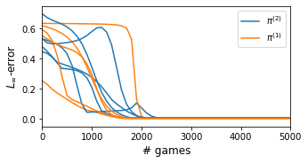
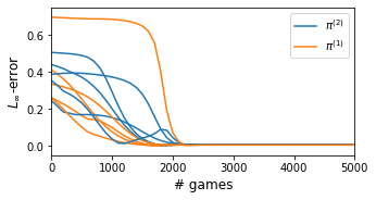
   Figure 3: Convergence in $\ell^{\infty}$-norm of 5 agents with random initialisation. Left: convergence of the policies parametrised with $\{e_{i};i=1,\ldots,4\}$. Right: convergence of the policies parametrised with $\{e_{i};i=1,\ldots,3\}$.

F.2 Control problems

For these problems, we use exponential decays for temperature $\tau$ and learning rate $\eta$, with prescribed terminal temperature $\tau_{T}$ and learning rate $\eta_{T}$. For example, for $\tau$ the decay rate is computed as $d_{\tau}=\left(\frac{\tau_{T}}{\tau_{0}}\right)^{1/ngames}$.

Frozen lake

The FrozenLake benchmark [9] is a $k\times k$ grid composed of cells, holes and one treasure. It features a discrete action space, namely, the agent can move in four directions (up, down, left, right). The episode terminates when the agent reaches the treasure or falls into a hole. We consider a $k=4$ for the numerical experiments. It is well-known that reshaping the reward function can change the performance of the algorithm. The original reward function does not discriminate between losing the game (falling into a hole), not moving and moving, so we will use a reshaped reward function: losing the game ($-1$), moving against a wall ($-0.1$), moving ($+0.01$) and reaching the treasure ($+10.0$).

For $k=4$, the optimal number of steps is $6$. We train sets of $5$ agents on $1000$ episodes. Then, the trained agents play $100$ games. For the MPG, we define a terminal $\tau_{T}=0.03$ and terminal learning rate $\eta_{T}=3\times 10^{-6}$, vary the initial learning rates $\eta$, temperatures $\tau$ and horizon to see the impact of these on the success of the agents. Similarly, for the VPG, we define a terminal $\tau_{T}=0.03$ and terminal learning rate $\eta_{T}=3\times 10^{-6}$. A summary of the results for horizons $n=10,15$ is given in table 1, showing that the policies obtained are optimal or very close to optimal. The column Failed to train denotes the policies that failed to converge (out of 5).

MPG $\tau_{0},~{}\eta_{0}$ Success (%) Average steps failed Horizon = 10 $0.15,~{}0.001$ 40.00 5.00 3 $0.15,~{}0.0005$ 40.00 6.00 3 $0.15,~{}0.0001$ 80.00 6.01 1 $0.15,~{}5\times 10^{-5}$ 39.80 5.37 3 $0.2,~{}0.001$ 20.00 6.00 4 $0.2,~{}0.0005$ 20.00 4.50 4 $0.2,~{}0.0001$ 40.00 5.00 3 $0.2,~{}5\times 10^{-5}$ 60.00 6.50 1 $0.3,~{}0.001$ 40.00 4.25 3 $0.3,~{}0.0005$ 51.60 6.14 2 $0.3,~{}0.0001$ 54.20 6.19 2 $0.3,~{}5\times 10^{-5}$ 0.00 - 5 $0.35,~{}0.001$ 100.00 6.00 0 $0.35,~{}0.0005$ 56.20 5.59 2 $0.35,~{}0.0001$ 38.80 6.77 3 $0.35,~{}5\times 10^{-5}$ 38.80 5.35 3 $0.4,~{}0.001$ 80.00 5.60 1 $0.4,~{}0.0005$ 80.00 6.30 1 $0.4,~{}0.0001$ 38.80 5.00 3 $0.4,~{}5\times 10^{-5}$ 39.80 5.54 3 Horizon = 15 $0.15,~{}0.001$ 40.00 4.19 3 $0.15,~{}0.0005$ 60.00 5.25 2 $0.15,~{}0.0001$ 60.00 5.25 2 $0.15,~{}5\times 10^{-5}$ 79.80 5.81 1 $0.2,~{}0.001$ 60.00 4.60 2 $0.2,~{}0.0005$ 75.00 5.25 1 $0.2,~{}0.0001$ 98.60 6.38 0 $0.2,~{}5\times 10^{-5}$ 79.80 5.43 1 $0.3,~{}0.001$ 60.00 4.92 2 $0.3,~{}0.0005$ 80.00 5.45 1 $0.3,~{}0.0001$ 60.00 5.66 2 $0.3,~{}5\times 10^{-5}$ 79.60 6.15 1 $0.35,~{}0.001$ 77.00 6.12 0 $0.35,~{}0.0005$ 100.00 6.00 0 $0.35,~{}0.0001$ 79.40 5.55 1 $0.35,~{}5\times 10^{-5}$ 59.80 5.35 2 $0.4,~{}0.001$ 100.00 6.00 0 $0.4,~{}0.0005$ 80.00 5.60 1 $0.4,~{}0.0001$ 100.00 6.15 0 $0.4,~{}5\times 10^{-5}$ 63.80 6.50 1   VPG $\tau_{0},~{}\eta_{0}$ Success (%) Average steps failed Horizon = 10 $0.15,~{}0.001$ 19.80 6.31 4 $0.15,~{}0.0005$ 20.00 6.00 4 $0.15,~{}0.0001$ 20.00 6.01 4 $0.15,~{}5\times 10^{-5}$ 38.40 6.14 3 $0.2,~{}0.001$ 0.00 - 5 $0.2,~{}0.0005$ 20.00 6.00 4 $0.2,~{}0.0001$ 0.00 - 5 $0.2,~{}5\times 10^{-5}$ 0.00 - 5 $0.3,~{}0.001$ 40.00 6.00 3 $0.3,~{}0.0005$ 20.00 6.04 4 $0.3,~{}0.0001$ 20.60 6.93 3 $0.3,~{}5\times 10^{-5}$ 7.60 7.00 4 $0.35,~{}0.001$ 60.00 6.03 2 $0.35,~{}0.0005$ 20.00 6.02 4 $0.35,~{}0.0001$ 1.20 9.33 2 $0.35,~{}5\times 10^{-5}$ 11.20 6.16 4 $0.4,~{}0.001$ 58.60 6.17 2 $0.4,~{}0.0005$ 100.00 6.06 0 $0.4,~{}0.0001$ 12.20 6.75 4 $0.4,~{}5\times 10^{-5}$ 0.20 9.00 4 Horizon = 15 $0.2,~{}0.001$ 20.00 6.00 4 $0.2,~{}0.0005$ 60.00 6.00 2 $0.2,~{}0.0001$ 36.80 6.40 3 $0.2,~{}5\times 10^{-5}$ 37.00 6.50 3 $0.25,~{}0.001$ 0.00 - 5 $0.25,~{}0.0005$ 79.80 6.00 1 $0.25,~{}0.0001$ 57.60 6.61 2 $0.25,~{}5\times 10^{-5}$ 36.40 7.01 3 $0.3,~{}0.001$ 0.00 - 5 $0.3,~{}0.0005$ 40.00 6.55 3 $0.3,~{}0.0001$ 40.60 8.80 1 $0.3,~{}5\times 10^{-5}$ 18.20 10.35 3 $0.35,~{}0.001$ 40.00 6.00 3 $0.35,~{}0.0005$ 30.40 6.97 3 $0.35,~{}0.0001$ 29.00 8.25 2 $0.35,~{}5\times 10^{-5}$ 41.20 8.71 2 $0.4,~{}0.001$ 54.60 6.91 1 $0.4,~{}0.0005$ 20.00 6.01 4 $0.4,~{}0.0001$ 55.20 7.10 1 $0.4,~{}5\times 10^{-5}$ 15.40 7.90 4

Table 1: Performance of trained agents on the Frozen Lake task on $4\times 4$ grid, for horizons $n=10,15$.

F.3 Cart Pole

The Cart Pole benchmark is a classical control problem. A pole is attached by an un-actuated joint to a cart, which moves along a frictionless track. The pole is placed upright on the cart, and the goal is to balance the pole by moving the cart to the left or right for some finite horizon time. It features a continuous environment and a discrete action space. The original reward function gives a $+1$ reward for each time that the pole stays upright, and the task finishes if the cart leaves the domain or if the pole is far enough from being upright. We reshape the reward function to give a penalty ($-10$) if the task is unsuccessful (i.e. the pole falls before reaching the target horizon).

We set the terminal $\tau=0.01$ and terminal learning rate $\eta=5\times 10^{-8}$. We train sets of $5$ agents on $2000$ episodes. Then, we play $100$ games with the trained agents and record the performance of the policies, as shown on table 2.

MPG $\tau_{0},~{}\eta_{0}$ Success (%) Average steps failed $0.1,~{}0.0001$ 35.80 65.62 0 $0.1,~{}1\times 10^{-5}$ 95.40 98.93 0 $0.15,~{}0.0001$ 77.40 91.65 0 $0.15,~{}1\times 10^{-5}$ 97.40 99.76 0 $0.2,~{}0.0001$ 86.20 97.66 0 $0.2,~{}1\times 10^{-5}$ 72.40 89.13 0   VPG $\tau_{0},~{}\eta_{0}$ Success (%) Average steps failed $0.1,~{}0.0001$ 23.00 42.33 0 $0.1,~{}1\times 10^{-5}$ 97.20 99.33 0 $0.15,~{}0.0001$ 31.80 53.44 0 $0.15,~{}1\times 10^{-5}$ 82.40 94.57 0 $0.2,~{}0.0001$ 49.00 61.86 0 $0.2,~{}1\times 10^{-5}$ 83.00 94.82 0

Table 2: Performance of trained agents on the CartPole task, for horizon $n=100$.

In practice, in order to achieve a more robust implementation, one could consider various stabilisation techniques such as gradient clipping to avoid updates which are too large or usage of off-policy updates, for example, through the use of a replay buffer. Other improvements to the training strategy can be adopted, such as: adaptive techniques to choose $\tau$ and $\eta$ during training can be considered, beyond the chosen continuous decay, batched trajectory updates, etc.

References

- [1] Alekh Agarwal, Sham M. Kakade, Jason D. Lee, and Gaurav Mahajan. On the theory of policy gradient methods: Optimality, approximation, and distribution shift. J. Mach. Learn. Res., 22(1), jul 2022.
- [2] Andréa Agazzi and Jianfeng Lu. Global optimality of softmax policy gradient with single hidden layer neural networks in the mean-field regime. ArXiv, abs/2010.11858, 2020.
- [3] Shun-ichi Amari. Information geometry and its applications, volume 194. Springer, 2016.
- [4] Kristopher De Asis, Alan Chan, Silviu Pitis, Richard S. Sutton, and Daniel Graves. Fixed-horizon temporal difference methods for stable reinforcement learning. ArXiv, abs/1909.03906, 2019.
- [5] Claude Berge. Topological spaces: Including a treatment of multi-valued functions, vector spaces and convexity. Oliver & Boyd, 1963.
- [6] Dimitri P. Bertsekas. Dynamic programming and optimal control. 1995.
- [7] Jalaj Bhandari and Daniel Russo. Global optimality guarantees for policy gradient methods. ArXiv, abs/1906.01786, 2019.
- [8] Jalaj Bhandari and Daniel Russo. On the linear convergence of policy gradient methods for finite mdps. In International Conference on Artificial Intelligence and Statistics, 2020.
- [9] Greg Brockman, Vicki Cheung, Ludwig Pettersson, Jonas Schneider, John Schulman, Jie Tang, and Wojciech Zaremba. Openai gym, 2016.
- [10] Tom B. Brown, Benjamin Mann, Nick Ryder, Melanie Subbiah, Jared Kaplan, Prafulla Dhariwal, Arvind Neelakantan, Pranav Shyam, Girish Sastry, Amanda Askell, Sandhini Agarwal, Ariel Herbert-Voss, Gretchen Krueger, T. J. Henighan, Rewon Child, Aditya Ramesh, Daniel M. Ziegler, Jeff Wu, Clemens Winter, Christopher Hesse, Mark Chen, Eric Sigler, Mateusz Litwin, Scott Gray, Benjamin Chess, Jack Clark, Christopher Berner, Sam McCandlish, Alec Radford, Ilya Sutskever, and Dario Amodei. Language models are few-shot learners. ArXiv, abs/2005.14165, 2020.
- [11] Shicong Cen, Chen Cheng, Yuxin Chen, Yuting Wei, and Yuejie Chi. Fast global convergence of natural policy gradient methods with entropy regularization. Oper. Res., 70:2563–2578, 2020.
- [12] Lénaïc Chizat and Francis R. Bach. A note on lazy training in supervised differentiable programming. ArXiv, abs/1812.07956, 2018.
- [13] Yuhao Ding, Junzi Zhang, and Javad Lavaei. Beyond exact gradients: Convergence of stochastic soft-max policy gradient methods with entropy regularization. ArXiv, abs/2110.10117, 2021.
- [14] Damien Ernst, Pierre Geurts, and Louis Wehenkel. Iteratively extending time horizon reinforcement learning. In Proceedings of the 14th European Conference on Machine Learning, ECML’03, page 96–107, Berlin, Heidelberg, 2003. Springer-Verlag.
- [15] Benjamin Eysenbach and Sergey Levine. If maxent rl is the answer, what is the question? ArXiv, abs/1910.01913, 2019.
- [16] Benjamin Eysenbach and Sergey Levine. Maximum entropy rl (provably) solves some robust rl problems. ArXiv, abs/2103.06257, 2021.
- [17] Maryam Fazel, Rong Ge, Sham M. Kakade, and Mehran Mesbahi. Global convergence of policy gradient methods for the linear quadratic regulator. In International Conference on Machine Learning, 2018.
- [18] KENJI Fukumizu. Infinite dimensional exponential families by reproducing kernel hilbert spaces. In 2nd International Symposium on Information Geometry and its Applications (IGAIA 2005), pages 324–333, 2005.
- [19] Soumyajit Guin and Shalabh Bhatnagar. A policy gradient approach for finite horizon constrained markov decision processes. ArXiv, abs/2210.04527, 2022.
- [20] Tuomas Haarnoja, Haoran Tang, P. Abbeel, and Sergey Levine. Reinforcement learning with deep energy-based policies. In International Conference on Machine Learning, 2017.
- [21] Tuomas Haarnoja, Aurick Zhou, P. Abbeel, and Sergey Levine. Soft actor-critic: Off-policy maximum entropy deep reinforcement learning with a stochastic actor. In International Conference on Machine Learning, 2018.
- [22] Tuomas Haarnoja, Aurick Zhou, Kristian Hartikainen, G. Tucker, Sehoon Ha, Jie Tan, Vikash Kumar, Henry Zhu, Abhishek Gupta, P. Abbeel, and Sergey Levine. Soft actor-critic algorithms and applications. ArXiv, abs/1812.05905, 2018.
- [23] Onésimo Hernández-Lerma and Jean Bernard Lasserre. Discrete-time markov control processes. 1999.
- [24] Arthur Jacot, Franck Gabriel, and Clément Hongler. Neural tangent kernel: Convergence and generalization in neural networks. In Proceedings of the 32nd International Conference on Neural Information Processing Systems, NIPS’18, page 8580–8589, Red Hook, NY, USA, 2018. Curran Associates Inc.
- [25] Arthur Jacot, Berfin Simsek, Francesco Spadaro, Clément Hongler, and Franck Gabriel. Implicit regularization of random feature models. ArXiv, abs/2002.08404, 2020.
- [26] James-Michael Leahy, Bekzhan Kerimkulov, David Siska, and Lukasz Szpruch. Convergence of policy gradient for entropy regularized MDPs with neural network approximation in the mean-field regime. In Kamalika Chaudhuri, Stefanie Jegelka, Le Song, Csaba Szepesvari, Gang Niu, and Sivan Sabato, editors, Proceedings of the 39th International Conference on Machine Learning, volume 162 of Proceedings of Machine Learning Research, pages 12222–12252. PMLR, 17–23 Jul 2022.
- [27] Sergey Levine. Reinforcement learning and control as probabilistic inference: Tutorial and review. ArXiv, abs/1805.00909, 2018.
- [28] Gen Li, Yuting Wei, Yuejie Chi, Yuantao Gu, and Yuxin Chen. Softmax policy gradient methods can take exponential time to converge. ArXiv, abs/2102.11270, 2021.
- [29] Timothy P. Lillicrap, Jonathan J. Hunt, Alexander Pritzel, Nicolas Manfred Otto Heess, Tom Erez, Yuval Tassa, David Silver, and Daan Wierstra. Continuous control with deep reinforcement learning. CoRR, abs/1509.02971, 2015.
- [30] Jincheng Mei, Chenjun Xiao, Csaba Szepesvari, and Dale Schuurmans. On the global convergence rates of softmax policy gradient methods. In International Conference on Machine Learning, 2020.
- [31] Ha Quang Minh, Partha Niyogi, and Yuan Yao. Mercer’s theorem, feature maps, and smoothing. In Learning Theory: 19th Annual Conference on Learning Theory, COLT 2006, Pittsburgh, PA, USA, June 22-25, 2006. Proceedings 19, pages 154–168. Springer, 2006.
- [32] Ofir Nachum, Mohammad Norouzi, Kelvin Xu, and Dale Schuurmans. Bridging the gap between value and policy based reinforcement learning. In Proceedings of the 31st International Conference on Neural Information Processing Systems, NIPS’17, page 2772–2782, Red Hook, NY, USA, 2017. Curran Associates Inc.
- [33] Brendan O’Donoghue, Rémi Munos, Koray Kavukcuoglu, and Volodymyr Mnih. Pgq: Combining policy gradient and q-learning. ArXiv, abs/1611.01626, 2016.
- [34] John Schulman, P. Abbeel, and Xi Chen. Equivalence between policy gradients and soft q-learning. ArXiv, abs/1704.06440, 2017.
- [35] John Schulman, Sergey Levine, P. Abbeel, Michael I. Jordan, and Philipp Moritz. Trust region policy optimization. ArXiv, abs/1502.05477, 2015.
- [36] John Schulman, Filip Wolski, Prafulla Dhariwal, Alec Radford, and Oleg Klimov. Proximal policy optimization algorithms. ArXiv, abs/1707.06347, 2017.
- [37] Richard S. Sutton and Andrew G. Barto. Reinforcement Learning: An Introduction. A Bradford Book, Cambridge, MA, USA, 2018.
- [38] Richard S. Sutton, David A. McAllester, Satinder Singh, and Y. Mansour. Policy gradient methods for reinforcement learning with function approximation. In NIPS, 1999.
- [39] Harm van Seijen, Mehdi Fatemi, and Arash Tavakoli. Using a logarithmic mapping to enable lower discount factors in reinforcement learning. In Neural Information Processing Systems, 2019.
- [40] Lingxiao Wang, Qi Cai, Zhuoran Yang, and Zhaoran Wang. Neural policy gradient methods: Global optimality and rates of convergence. ArXiv, abs/1909.01150, 2019.
- [41] Lilian Weng. Policy gradient algorithms. lilianweng.github.io, 2018.
- [42] Ronald J. Williams. Simple statistical gradient-following algorithms for connectionist reinforcement learning. Machine Learning, 8:229–256, 1992.
- [43] Junzi Zhang, Jongho Kim, Brendan O’Donoghue, and Stephen Boyd. Sample efficient reinforcement learning with reinforce. In AAAI Conference on Artificial Intelligence, 2020.
- [44] K. Zhang, Alec Koppel, Haoqi Zhu, and Tamer Başar. Global convergence of policy gradient methods to (almost) locally optimal policies. SIAM J. Control. Optim., 58:3586–3612, 2019.