Kerr binary dynamics from minimal coupling and double copy
Francesco Alessio^a,b

^a NORDITA, KTH Royal Institute of Technology and Stockholm University,
Hannes Alfvéns väg 12, SE-11419 Stockholm, Sweden
^b Department of Physics and Astronomy, Uppsala University,
Box 516, SE-75120 Uppsala, Sweden

We construct a new Yang-Mills Lagrangian based on a notion of minimal coupling that incorporates classical spin effects. The construction relies on the introduction of a new covariant derivative, which we name “classical spin covariant derivative”, that is compatible with the three-point interaction of the $\sqrt{\mathrm{Kerr}}$ solution with the gauge field. The resulting Lagrangian, besides the correct three-point coupling, predicts a unique choice for contact terms and therefore it can be used to compute higher-point amplitudes such as the Compton, unaffected by spurious poles. Using double copy techniques we use this theory to extract gravity amplitudes and observables that are relevant to describe Kerr binary dynamics to all orders in the spin. In particular, we compute the 2PM ($\mathcal{O}(G^{2}_{N})$) $2\rightarrow 2$ elastic scattering amplitude between two classically spinning objects to all orders in the spin and use it to extract the 2PM scattering angle.

1 Introduction

The idea that black holes share certain features with elementary particles is not new and, in fact, it has quite a long history (see e.g.[1, 2, 3]). One of the reasons that makes these two classes of apparently unrelated objects similar is that they are both characterized by few charges, namely the mass, the intrinsic angular momentum i.e. the spin and the electric charge. Although being exact solutions of the full, non-linear Einstein equations, black holes seem to be simple objects, at least if compared to other solutions such as neutron stars.

Beside being interesting in itself, the aforementioned analogy can be concretely used to perform analytical precision computations relevant in the context of gravitational waves physics, that has recently dragged a lot of attention because of the many detections made by LIGO, Virgo and Kagra of waves emitted by strongly gravitating binary systems [4, 5, 6, 7, 8, 9, 10] . During the very first phase of the coalescence of two black holes, known as the inspiral phase, the two compact objects are widely separated and the gravitational interaction between them is weak. In this regime one can neglect the internal structure of the bodies, sized by the Schwarzschild radius, and successfully use perturbation theory to extract the perturbative expansion in the gravitational coupling constant of the observables one is interested in. This is called post-Minkowskian (PM) regime and it is usually approached either by using classical general relativity (GR) methods or scattering amplitude techniques in quantum field theory (QFT) [11, 12, 13, 14, 15, 16, 17, 18, 19, 20, 21, 22, 23, 24, 25, 26, 27, 28, 29, 30, 31, 32, 33, 34, 35, 36, 37, 38, 39, 40, 41, 42, 43, 44, 45, 46, 47, 48, 49, 50, 51, 52, 53, 54, 55, 56, 57, 58]. However, because of on-shell techniques and many simplifications, state-of-the-art theoretical predictions are made within the latter approach, where one treats the two gravitating bodies as elementary point-like particles, computes a scattering amplitude and then extracts its classical limit, which roughly amounts to sending $\hbar$ to zero, after having correctly restored it in the theory. Eventually open orbits observables, obtained by differentiating the classical scattering amplitude, can be mapped into bounded orbits ones [59, 60, 61] and can be compared to those derived in the more familiar Post-Newtonian (PN) regime (see e.g. [62] for a review), where, together with the weak field approximation, one also considers small velocities.

It is not surprising that the theory used to describe the gravitational interaction between Schwarzschild black holes, only characterized by their masses, is in the PM regime simply that of minimally coupled massive scalars to gravity. Computations can be significantly simplified using double copy [63, 64, 65, 66, 67] and, infact, it has been shown that scalar QCD provides the single copy theory to compute the relevant building blocks and amplitudes for the the more complicated theory of gravity [68, 69, 15, 3, 70, 71, 72, 73]. State-of-the-art results for the scattering between two spinless black holes in both the conservative and radiative sectors are up to 4PM ($\mathcal{O}(G^{4}_{N})$).

However, more realistic black holes are also characterized by the spin vector $S^{\mu}$ [74]. Because of this additional scale the problem is much more complicated and, on top of each PM order, there is a spin multipole expansion in the classical spin vector that, in general, depends on the nature of the compact body one is describing [75, 76, 77, 78, 79, 80, 81, 82, 83, 84, 85, 86, 87, 88, 89, 90, 91, 92, 93, 94, 95, 96, 97, 98, 99, 100, 101, 102, 103, 104, 105, 106, 107, 108, 109, 110, 111, 112, 113, 114, 115, 116, 117, 118, 119, 120, 121, 122, 123, 124, 125, 126, 127, 128, 129, 130, 131, 132, 133]. Quantum-mechanically, the spin vector satisfies $S^{\mu}S_{\mu}=-\hbar^{2}s(s+1)$, where $s$ is the spin quantum number. Hence, when trying to attack the classical scattering problem using QFT methods, it seems natural to make use of spinning massive fields, with higher and higher value of the spin quantum number $s$ , in such a way to keep the value of $S^{\mu}S_{\mu}$ finite when sending $\hbar$ to zero. This will yield a spin multipole expansion in the form of a polynomial truncated at order $(S^{\mu})^{2s}$. The idea of using quantum spinning fields to mimic Kerr black holes is corroborated by the “minimally coupled” three-point amplitudes presented in [75] that, in the classical limit, match the classical computation of the linearised stress-energy tensor of a Kerr black hole [78]. The latter resums all the classical spin dependence of the amplitude into a simple and compact exponentiated form that can be interpreted, on the support of the three-point kinematics, as an exponentiated version of the subleading soft graviton theorem [81, 134]. Using this three-point amplitude, the 1PM classical amplitude for the scattering between two Kerr black holes has been easily constructed to all order in spin [81, 86]. However, going to 2PM requires the knowledge of the tree-level Compton amplitude and, when one constructs such object using BCFW recursion relations [135], the opposite-helicity sector is affected, for $s>2$, i.e. for higher spins, by the presence of unphysical spurious poles. The same problem appears for gauge theories when $s>1$, when starting from the $\sqrt{\mathrm{Kerr}}$ three-point amplitude. There has been a lot of effort to understand how to remove these poles. The Lagrangian approaches of [102, 112] give healthy Compton amplitudes up to $s=5/2$. Assuming that the Compton amplitude additionally satisfies a “shift-symmetry” to all orders in spin leads to a result unaffected by the above-mentioned spurious poles [110]. A microscopical reason for assuming such symmetry is, however, far from being clear. All these efforts and proposals should eventually be compared with solutions of the classical Teukolsky equation, recently found in [125].

In this paper, we follow a different path. We try to answer the question of whether it is possible, in principle, to construct an effective Lagrangian field theory describing the interactions of Kerr black holes with gravity depending on the classical spin $S^{\mu}$ and therefore carrying, as a built-in feature, an infinite spin multipole expansion. There are several motivations to ask this question. The first is of purely theoretical nature. As argued above, black holes are, from a certain perspective, simple and this simplicity, for the Schwarzschild case, is reflected in the standard QFT notion of minimal coupling. On the other hand, Kerr black-holes look much more sophisticated but they are actually not, as clear in Kerr-Schild coordinates [136]. Indeed, Kerr spacetime can be entirely reconstructed by performing a Newman-Janis transformation [137] to the radial coordinate characterizing the spinless solution. Constructing a new field theory for Kerr by implementing this transformation directly at the level of the Lagrangian would represent at least a good candidate to describe Kerr black holes as elementary particles. A second, but not less important, motivation concerns the frontier of precision computations. Having a Lagrangian built upon the criterion of simplicity would make it possible to proceed beyond the first PM order in the perturbative expansion of gravitational observables. One could argue that, unless there is a classical GR computation that counterparts the analysis of this paper, these observables could have little to do with Kerr black holes. However, in any case, the theory we present here could always be regarded as a “minimal” model on top of which one is free to add operators of higher order in the curvature, opportunely multiplied by Wilson coefficients, in order to better and better approximate true classically spinning solutions.

In practice we do not construct here the theory of gravity, but we limit ourselves to build its single copy, gauge theory counterpart. Then, implementing a form of the double copy that adapts to classically spinning theories, we obtain gravity amplitudes.

The paper is organized as follows. We start in section 2 where, after discussing the usual notion of minimal coupling and its role in scalar QED, we construct a new theory by introducing a covariant derivative which is compatible with the $\sqrt{\mathrm{Kerr}}$ three-point amplitude and that carries information about its interaction with the gauge field. We show explicit expressions for the Lagrangian and for the contact terms, automatically generated by this definition of minimal coupling. The Newman-Janis shift, discussed in some detail in appendix A, is a constitutive element of our Lagrangian. In section 3 we consider tree-level amplitudes and we show that, on-shell, spinning amplitudes involving an arbitrary number of massless legs entirely factorize in terms of spinless ones and that the full spin contribution can remarkably be encoded into a simple exponential factor. Because they come from a local Lagrangian, such amplitudes will be unaffected by unphysical poles. The difference between the opposite-helicity Compton amplitude we find within our approach and the “minimally coupled” one is spelled out in appendix B. Using double copy for classically spinning theories, in section 4, we obtain gravity amplitudes relevant to describe Kerr black holes binary dynamics. Section 5 is devoted to the computation of the 2PM amplitude, eikonal and scattering angle using on-shell techniques. Integrals appearing in the one-loop amplitude and eikonal are computed in appendix D and E. We conclude in 6 with a discussion. Throughout the paper we use mostly minus signature.

2 Minimal coupling and classical spin

In this section we start by considering scalar QED, review its Feynman rules and compute the well-known Compton amplitude. Afterwards, by analogy and requiring compatibility with the three-point coupling of the $\sqrt{\mathrm{Kerr}}$ solution, we build a new Lagrangian describing classically spinning scalars coupled to the electromagnetic field.

Scalar QED

A scalar $\phi$ with mass $m$ and electric charge $e$ minimally coupled to the electromagnetic field is described by the scalar QED Lagrangian,

$$\mathcal{L}=-\frac{1}{4}F_{\mu\nu}F^{\mu\nu}+(D_{\mu}\phi)^{*}(D^{\mu}\phi)-m^{2}|\phi|^{2},\hskip 14.22636ptD_{\mu}=\partial_{\mu}+ieA_{\mu}.$$ (2.1)

Under gauge transformations,

$$A_{\mu}\rightarrow A_{\mu}-\frac{i}{e}U\partial_{\mu}U^{*},\hskip 28.45274pt\phi\rightarrow U\phi,\hskip 28.45274ptU=e^{ie\hskip 1.42271pt\chi}\in U(1),$$ (2.2)

the covariant derivative transforms as $D_{\mu}\phi=UD_{\mu}\phi$. This is the usual QFT notion of minimal coupling, that consists in providing interactions between matter and gauge fields with the least number of derivatives in a gauge invariant way. Clearly other non-minimal interaction terms, containing more derivatives, may be added to the Lagrangian, but we will not consider them here. Beside ensuring gauge invariance, the replacement $\partial_{\mu}\phi\rightarrow D_{\mu}\phi$ in the free Lagrangian automatically yields three- and four-point couplings,

$$\mathcal{L}_{3\mathrm{pt}}=ieA^{\mu}(\phi\partial_{\mu}\phi^{*}-\phi^{*}\partial_{\mu}\phi),\qquad\mathcal{L}_{4\mathrm{pt}}=e^{2}A^{\mu}A_{\mu}|\phi|^{2},$$ (2.3)

from which we easily read the Feynman rules,

$$\vbox{\hbox{\includegraphics[width=102.43008pt,height=113.81102pt]{3pt.png}}}\begin{aligned} \hskip 2.84544pt=-ie\hskip 1.42271ptp^{\mu},\end{aligned}\begin{aligned} \hskip 56.9055pt\vbox{\hbox{\includegraphics[width=102.43008pt,height=113.81102pt]{ct.png}}}\hskip 2.84544pt=2ie^{2}\eta^{\mu\nu},\end{aligned}$$ (2.4)

where $\phi$ ($\phi^{*}$) has momentum $p_{1}$ ($p_{2}$), $p\equiv p_{2}-p_{1}$ and where, by total momentum conservation for the first diagram $p_{1}+p_{2}+q=0$ and for the second $p_{1}+q_{1}+q_{2}+p_{4}=0$. The tree-level Compton amplitude is the sum of the three diagrams below,

$$i\mathcal{A}^{\mu\nu}_{4}(p_{i},q_{i})=\vbox{\hbox{\includegraphics[width=82.51282pt,height=110.96556pt]{C.png}}}\begin{aligned} \hskip 2.84544pt=\end{aligned}\vbox{\hbox{\includegraphics[width=71.13188pt,height=110.96556pt]{g1.png}}}\hskip 2.84544pt\begin{aligned} +\end{aligned}\vbox{\hbox{\includegraphics[width=71.13188pt,height=110.96556pt]{g2.png}}}\hskip 2.84544pt\begin{aligned} +\end{aligned}\vbox{\hbox{\includegraphics[width=71.13188pt,height=110.96556pt]{g3.png}}}.$$ (2.5)

Using the scalar propagator, we get for $\mathcal{A}_{4}^{\mu\nu}$,

$$\mathcal{A}^{\mu\nu}_{4}(p_{i},q_{i})=-2e^{2}\bigg{(}\frac{p_{1}^{\mu}p_{1}^{\nu}+q_{2}^{\mu}p_{1}^{\nu}}{p_{1}\cdot q_{2}}+\frac{p_{1}^{\mu}p_{1}^{\nu}+p_{1}^{\mu}q_{3}^{\nu}}{p_{1}\cdot q_{3}}-\eta^{\mu\nu}\bigg{)}.$$ (2.6)

Contracting with physical polarization vectors satisfying $\varepsilon_{i}^{2}=0=\varepsilon_{i}\cdot q_{i}$ and using the on-shell conditions $q^{2}_{i}=0$ we get,

$$\mathcal{A}_{4}(p_{i},q_{i})\equiv\varepsilon_{1\nu}\varepsilon_{2\mu}\mathcal{A}^{\mu\nu}_{4}(p_{i},q_{i})=-\frac{2e^{2}}{p_{1}\cdot q_{2}p_{1}\cdot q_{3}}p_{1}\cdot F_{2}\cdot F_{3}\cdot p_{1},$$ (2.7)

where we introduced the field strength $F_{i}^{\mu\nu}=2\varepsilon_{i}^{[\mu}q_{i}^{\nu]}$ and used that, on-shell, $p_{1}\cdot(q_{2}+q_{3})=-q_{2}\cdot q_{3}$. Note that $\mathcal{A}_{4}$ is gauge invariant because it is written purely in terms of gauge invariant field strengths. If we knew only the three-point coupling in equation (2.3) i.e. if we summed only the first two diagrams in (2.5), we could have guessed the four-point contact term, necessary to achieve gauge invariance, just by requiring that $\delta_{\chi}\mathcal{A}_{4}=0$. This suggests that, in a minimally coupled gauge theory, contact terms are always generated as a consequence of the three-point coupling that, in turn, comes from the notion of a “good” covariant derivative.

As widely discussed in the literature and in the introduction, amplitudes describing Schwarzschild black holes come from minimally coupled scalars to gravity. Such minimal coupling is, at the gauge theory level, encoded in the notion of covariant derivative and indeed, the classical Compton amplitude for Schwarzschild black holes can be simply obtained by double copying $\mathcal{A}_{4}$ in (2.7). This shows that the simplicity of black holes is intimately connected to the notion of minimal coupling. In the following we will assume, relying on the considerations of the previous section and in particular on the Newman-Janis algorithm, discussed in appendix A, that Kerr black holes should also be described by a minimally coupled, simple, theory. In other words, we will ask whether the classical three-point amplitude for $\sqrt{\mathrm{Kerr}}$, known to all orders in the spin, yields a good covariant derivative and can therefore be used to generate contact terms in the same way they are derived in the spinless case. The answer to this question, quite surprisingly, is yes.

$\sqrt{\mathrm{Kerr}}$ and classically spinning gauge theory

In the worldline picture, the Coulomb field can be thought of as generated by a charged scalar sourced by a static point particle and hence it is a solution of the Maxwell equations,

$$\partial_{\mu}F^{\mu\nu}(x)=J^{\nu}(x),\qquad J^{\mu}(x)=e\int\frac{d\tau}{2\pi}u^{\mu}\delta^{(4)}(x-u\tau),$$ (2.8)

where $\tau$ is the proper time of the point particle moving on the worldline $x(\tau)$ and $u^{\mu}(\tau)=\dot{x}(\tau)$ is the unit tangent vector to the curve satisfying $u_{\mu}u^{\mu}=1$ (see e.g. [70]). Taking the Fourier transform of $J^{\mu}(x)$ yields,

$$\tilde{J}^{\mu}(q)=\int\frac{d^{4}x}{(2\pi)^{4}}e^{iq\cdot x}J^{\mu}(x)=e\hskip 1.42271ptu^{\mu}\delta(q\cdot u).$$ (2.9)

From a Lagrangian field theory point of view, the coupling of the charged particle to the electromagnetic field is encoded in the term $A_{\mu}J^{\mu}$ and therefore the Feynman rule for the three-point amplitude is the Fourier transform $\tilde{J}^{\nu}(q)$ of $J^{\nu}(x)$. Indeed, introducing $p^{\mu}=mu^{\mu}$ the Fourier transform (2.9) is proportional to the first equation in (2.4). The additional delta function appearing in (2.9) enforces three-point kinematics $p_{1}\cdot q=p_{2}\cdot q=p\cdot q=0$.

As shown in the context of gravity in [78], the $\sqrt{\mathrm{Kerr}}$ solution, which is the electromagnetic field generated by a rotating disc of radius $a$, is sourced by the following current,

$$J^{\mu}(x)=e\int\frac{d\tau}{2\pi}\mathrm{exp}\{\epsilon^{\mu}{}_{\nu}(a,\partial)\}u^{\nu}\delta^{(4)}(x-u\tau),\qquad\epsilon^{\mu}{}_{\nu}(a,\partial)\equiv\epsilon^{\mu}{}_{\nu\rho\sigma}a^{\rho}\partial^{\sigma},$$ (2.10)

where the rescaled spin vector $a^{\mu}$ is related to the classical Pauli-Lubanski spin vector $S^{\mu}$ by $S^{\mu}=ma^{\mu}$ and satisfies the Tulczjew-Dixon SSC condition $a\cdot u=0$ [138, 139]. This time, performing the Fourier transform yields [81],

$$\tilde{J}^{\mu}(q)=\int\frac{d^{4}x}{(2\pi)^{4}}e^{iq\cdot x}J^{\mu}(x)=e\hskip 1.42271pt\mathrm{exp}\{i\epsilon^{\mu}{}_{\nu}(a,q)\}u^{\nu}\delta(q\cdot u),$$ (2.11)

which leads to the following three-point amplitude,

$$\vbox{\hbox{\includegraphics[width=102.43008pt,height=113.81102pt]{3pt.png}}}\begin{aligned} \hskip 2.84544pt=-ie\hskip 1.42271pt\mathrm{exp}\{i\epsilon^{\mu}{}_{\nu}(a,q)\}p^{\nu}\equiv-ie\hskip 1.42271pt\Lambda^{\mu}{}_{\nu}(a,q)p^{\nu}.\end{aligned}$$ (2.12)

In practice, switching from scalar QED to $\sqrt{\mathrm{Kerr}}$ amounts to multiplying the three-point Feynman rule of the former by a matrix $\Lambda^{\mu}{}_{\nu}(a,q)$, which is the exponential of the antisymmetric tensor $\omega_{\mu\nu}=-\omega_{\nu\mu}=\epsilon_{\mu\nu}(a,q)$. Remarkably, it was shown in [81, 86] that the amplitude (2.12) corresponds to the classical limit of “minimally coupled” three-point amplitudes constructed in [75]. Indeed, contracting (2.12) with $\varepsilon_{\mu}$ and expanding the exponential gives,

$$-ie\hskip 1.42271pt\varepsilon^{\mu}\bigg{[}\eta_{\mu\nu}+i\epsilon_{\mu\nu}(a,q)-\frac{1}{2!}\epsilon_{\mu\gamma}(a,q)\epsilon^{\gamma}{}_{\nu}(a,q)+\dots\bigg{]}p^{\nu}$$

$$= ie\hskip 1.42271pt\varepsilon\cdot p\bigg{[}1+i\frac{\varepsilon\cdot S\cdot q}{\varepsilon\cdot p}+\frac{1}{2}(a\cdot q)^{2}+\dots\bigg{]}=ie\hskip 1.42271pt\varepsilon\cdot p\hskip 1.42271pt\mathrm{exp}\left\{\frac{i}{2}\frac{S^{\mu\nu}F_{\mu\nu}}{\varepsilon\cdot p}\right\},$$ (2.13)

where $S^{\mu\nu}=\epsilon^{\mu\nu\alpha\beta}p_{\alpha}a_{\beta}$ is the spin tensor of the massive particle and where we repeatedly used the relations,

$$\epsilon^{\mu\nu\rho\sigma}\epsilon_{\alpha\beta\gamma\delta}=-4!\delta^{[\mu}_{\alpha}\delta^{\nu}_{\beta}\delta^{\rho}_{\gamma}\delta^{\sigma]}_{\delta},\qquad\epsilon^{\mu\nu\rho\lambda}\epsilon_{\alpha\beta\gamma\lambda}=-3!\delta^{[\mu}_{\alpha}\delta^{\nu}_{\beta}\delta^{\rho]}_{\gamma},$$ (2.14)

together with, crucially, the three-point kinematics $p\cdot q=0$, the on-shell conditions $\varepsilon^{2}=q^{2}=\varepsilon\cdot q=0$ and the SSC $a\cdot p=0$ as well. It is suggestive to note [81] that the exponential factor appearing in (2) is exactly an exponentiated version of the subleading soft photon theorem [140]. The poles appearing when expanding the exponential in (2) for $a>1$ are cancelled due to three-point kinematics,

$$\frac{i}{2}\frac{S^{\mu\nu}F_{\mu\nu}}{\varepsilon\cdot p}=i\frac{\varepsilon\cdot S\cdot q}{\varepsilon\cdot p}=-\frac{a\cdot\varepsilon\hskip 1.42271ptp\cdot q-a\cdot q\hskip 1.42271ptp\cdot\varepsilon}{p\cdot\varepsilon}=a\cdot q,$$ (2.15)

where we used $\varepsilon\cdot S\cdot q=\sqrt{(\varepsilon\cdot S\cdot q)^{2}}$ and the Gram determinants in (2.14) with the assumption of real polarization vector $\varepsilon$.

Asking that the structure appearing in (2.12) comes from a standard QFT notion of minimal coupling, i.e. from the existence of a covariant derivative, implies that the latter should be,

$$D_{\mu}^{(a)}=\partial_{\mu}-ie\hskip 1.42271pt\mathrm{exp}\{\epsilon^{\nu}{}_{\mu}(a,\partial)\}A_{\nu}.$$ (2.16)

Under gauge transformations as in (2.2) we have,

$$D_{\mu}^{(a)}\phi\rightarrow \partial_{\mu}(U\phi)-ie\hskip 1.42271pt\mathrm{exp}\{\epsilon^{\nu}{}_{\mu}(a,\partial)\}(A_{\nu}+\partial_{\nu}\chi)(U\phi)=UD_{\mu}^{(a)}\phi,$$ (2.17)

where we used that the matrix exponential acts trivially on pure gauge configurations, $\mathrm{exp}\{\epsilon^{\nu}{}_{\mu}(a,\partial)\}\partial_{\nu}\chi=\partial_{\mu}\chi$. Equation (2.17) shows that the operator $D_{\mu}^{(a)}$ is indeed a good covariant derivative and it can be used to construct consistent interactions between matter and gauge fields. We will denote $D_{\mu}^{(a)}$ as classical spin covariant derivative. We are naturally led to consider the gauge invariant Lagrangian,

$$\mathcal{L}=-\frac{1}{4}F_{\mu\nu}F^{\mu\nu}+(D^{(a)}_{\mu}\phi)^{*}(D^{\mu}_{(a)}\phi)-m^{2}|\phi|^{2}=\mathcal{L}_{\mathrm{free}}+\mathcal{L}_{3\mathrm{pt}}+\mathcal{L}_{4\mathrm{pt}},$$ (2.18)

where,

$$\mathcal{L}_{3\mathrm{pt}}=ie\hskip 1.42271pt\mathrm{exp}\{\epsilon_{\mu\nu}(a,\partial)\}A^{\mu}(\phi\partial^{\nu}\phi^{*}-\phi^{*}\partial^{\nu}\phi),$$ (2.19)

$$\mathcal{L}_{4\mathrm{pt}}=e^{2}\mathrm{exp}\{\epsilon_{\mu\rho}(a,\partial)\}A^{\mu}\mathrm{exp}\{\epsilon_{\nu}{}^{\rho}(a,\partial)\}A^{\nu}|\phi|^{2},$$ (2.20)

that automatically yields the three-point diagram in (2.12) and the four-point contact term,

$$\vbox{\hbox{\includegraphics[width=102.43008pt,height=113.81102pt]{ct.png}}}\hskip 2.84544pt=2ie^{2}\Lambda^{\mu}{}_{\rho}(a,q_{3})\Lambda^{\nu\rho}(a,q_{2}).$$ (2.21)

Before proceeding further we note here that, in general, the field strength is defined as the commutator of covariant derivatives, $F_{\mu\nu}=\frac{i}{e}[D_{\mu},D_{\nu}]$. Using this definition, together with the classical spin connection in (2.16), would change the photon propagator. However, in the theory (2.18) we are keeping the free part as it is in the standard YM Lagrangian, without modifying the field strength as $F_{\mu\nu}\rightarrow F^{(a)}_{\mu\nu}$. In other words, the photon field gets dressed with the spin exponential matrix only when it interacts locally with the massive, classically spinning field $\phi$. Away from it photons are not affected by the spin. This remark is not important in the abelian version of the theory we are presenting here, because none of the diagrams appearing in the Compton (2.5) contains a photon propagator. When extending this theory to gluons, however, beside the two massive channels and the contact term, there is also a massless channel involving the gluon propagator.

It comes as a consequence of the above considerations that the spinning Compton amplitude $\mathcal{A}_{4}^{\mu\nu}(a)$ is simply factorized in terms of the spinless one as,

$$\mathcal{A}_{4}^{\mu\nu}(a;p_{i},q_{i})=\Lambda^{\mu}{}_{\rho}(a,q_{3})\Lambda^{\nu}{}_{\sigma}(a,q_{2})\mathcal{A}_{4}^{\rho\sigma}(p_{i},q_{i}).$$ (2.22)

We need to contract with polarization vectors $\varepsilon_{2\nu}$ and $\varepsilon_{3\mu}$ and hence it is convenient to define new vectors $\varepsilon^{\prime\mu}_{i}=\Lambda_{\nu}{}^{\mu}(a,q_{i})\varepsilon^{\nu}_{i}$ so that,

$$\mathcal{A}_{4}(a;p_{i},q_{i})=\varepsilon_{2\nu}\varepsilon_{3\mu}\mathcal{A}_{4}^{\mu\nu}(a;p_{i},q_{i})=-\frac{2e^{2}}{p_{1}\cdot q_{2}p_{1}\cdot q_{3}}p_{1}\cdot F^{\prime}_{2}\cdot F^{\prime}_{3}\cdot p_{1},$$ (2.23)

where $F_{i}^{\prime\mu\nu}=2\varepsilon^{\prime[\mu}_{i}q_{i}^{\nu]}$. In general, all the spinning tree-level amplitudes $\mathcal{A}_{N}^{\mu_{2}\dots\mu_{N-1}}(a)$ involving two massive and $N-2$ massless lines with momenta $q_{2},\dots,q_{N-1}$ following from the Lagrangian (2.18) can be written in terms of the spinless ones as,

$$\mathcal{A}^{\mu_{2}\dots\mu_{N-1}}_{N}(a;p_{i},q_{i})=\vbox{\hbox{\includegraphics[width=96.73918pt,height=113.81102pt]{nC.png}}}\\ \begin{aligned} \hskip 2.84544pt=\Lambda^{\mu_{2}}{}_{\nu_{2}}(a,q_{2})\dots&\Lambda^{\mu_{N-1}}{}_{\nu_{N-1}}(a,q_{N-1})\\ &\mathcal{A}_{N}^{\nu_{2}\dots\nu_{N-1}}(p_{i},q_{i}).\end{aligned}$$ (2.24)

3 Spin exponentiation

The Lagrangian presented in the previous section predicts tree-level spinning amplitudes containing various factors of $\Lambda_{\nu}{}^{\mu}(a,q_{i})\varepsilon^{\nu}_{i}$ for each external massless line. Here we would like to analyse these factors more in detail and to extract an alternative expression that possibly does not contain the Levi-Civita symbol. We introduce the shorthand notation $\epsilon^{\mu_{1}\dots\mu_{n}}{}_{\nu_{1}\dots\nu_{n}}v^{\nu_{1}}_{1}\dots v^{\nu_{m}}_{m}\equiv\epsilon^{\mu_{1}\dots\mu_{n}}(v_{1},\dots,v_{m})$ for $m$ vectors $v_{1},\dots,v_{m}$, that generalizes the one used in (2.10) and we start by expanding the exponential as,

$$\mathrm{exp}\{i\epsilon_{\nu}{}^{\mu}(a,q)\}\varepsilon^{\nu}=\hskip 1.42271pt \varepsilon^{\mu}-i\epsilon^{\mu}(\varepsilon,a,q)+\frac{1}{2!}\epsilon^{\alpha}(\varepsilon,a,q)\epsilon_{\alpha}{}^{\mu}(a,q)$$

$$+ \frac{i}{3!}\epsilon^{\alpha}(\varepsilon,a,q)\epsilon_{\alpha}{}^{\beta}(a,q)\epsilon_{\beta}{}^{\mu}(a,q)+\dots$$ (3.1)

Defining the dual field strength $F^{*\mu\nu}_{i}=\frac{i}{2}\epsilon^{\mu\nu}{}_{\rho\sigma}F^{\rho\sigma}=i\epsilon^{\mu\nu}(\varepsilon,q)$ and using the on-shell equality,

$$\epsilon^{\alpha}(\varepsilon,a,q)\epsilon_{\alpha}{}^{\beta}(a,q)=a\cdot q(a\cdot q\varepsilon^{\beta}-a\cdot\varepsilon q^{\beta})=a\cdot qF^{\beta\rho}a_{\rho},$$ (3.2)

the series in (3) can easily be resummed,

$$\mathrm{exp}\{i\epsilon_{\nu}{}^{\mu}(a,q)\}\varepsilon^{\nu}=\hskip 1.42271pt \varepsilon^{\mu}+F^{*\mu\rho}a_{\rho}+\frac{1}{2!}(a\cdot q_{i})a_{\rho}F^{\mu\rho}+\frac{1}{3!}(a\cdot q)^{2}F^{*\mu\rho}a_{\rho}+\dots$$

$$=\hskip 1.42271pt \frac{a\cdot\varepsilon}{a\cdot q}q^{\mu}+\frac{F^{*\mu\rho}a_{\rho}}{a\cdot q}\sinh(a\cdot q)+\frac{F^{\mu\rho}a_{\rho}}{a\cdot q}\cosh(a\cdot q).$$ (3.3)

So far, we have not specified the helicity of the massless state $\varepsilon$. A field strength admits a decomposition into its positive and negative helicity components $F^{\mu\nu}_{h}$ with $h=\pm$ [73],

$$F^{+}_{\mu\nu}=\frac{1}{2}(F_{\mu\nu}-F^{*}_{\mu\nu}),\qquad F^{-}_{\mu\nu}=\frac{1}{2}(F_{\mu\nu}+F^{*}_{\mu\nu}),$$ (3.4)

that, plugged into (3) yields,

$$\mathrm{exp}\{i\epsilon_{\nu}{}^{\mu}(a,q)\}\varepsilon^{\nu}=\frac{a\cdot\varepsilon}{a\cdot q}q^{\mu}+\frac{F_{+}^{\mu\rho}a_{\rho}}{a\cdot q}e^{-a\cdot q}+\frac{F_{-}^{\mu\rho}a_{\rho}}{a\cdot q}e^{a\cdot q}.$$ (3.5)

Therefore for fixed helicity $h$ we find,

$$\mathrm{exp}\{i\epsilon_{\nu}{}^{\mu}(a,q)\}\varepsilon^{\nu}_{h}=e^{-ha\cdot q}\varepsilon^{\mu}_{h}-\frac{(e^{-ha\cdot q}-1)}{a\cdot q}a\cdot\varepsilon_{h}q^{\mu},\qquad h=\pm.$$ (3.6)

We conclude that, up to a gauge transformation, positive and negative helicity vectors are eigenvectors of the operator $\mathrm{exp}\{i\epsilon_{\nu}{}^{\mu}(a,q)\}$ with eigenvalues $e^{-ha\cdot q}$. An immediate consequence is that the spinning three-point amplitude in (2.12), on-shell ($p\cdot q=0$) and once specified the helicity of the emitted photon, reads simply $(p\cdot\varepsilon_{h})e^{-ha\cdot q}$. More in general, any tree-level gauge invariant amplitude of the form (2.24) will contain a product of spin exponentials,

$$\mathcal{A}^{h_{2}\dots h_{N-1}}_{N}(a;p_{i},q_{i}) =\epsilon^{h_{2}}_{\mu_{2}}\Lambda^{\mu_{2}}{}_{\nu_{2}}(a,q_{2})\dots\epsilon^{h_{N-1}}_{\mu_{N-1}}\Lambda^{\mu_{N-1}}{}_{\nu_{N-1}}(a,q_{N-1})\mathcal{A}_{N}^{\nu_{2}\dots\nu_{N-1}}(p_{i},q_{i})$$

$$=e^{-\sum_{i=2}^{N-1}h_{i}\hskip 0.28436pta\cdot q_{i}}\mathcal{A}^{h_{2}\dots h_{N-1}}_{N}(p_{i},q_{i}).$$ (3.7)

In particular, for $N=4$, i.e. for the Compton amplitude, the equal- and opposite-helicity sectors are,

$$\mathcal{A}_{4}^{\pm\pm}(a;p_{i},q_{i})=e^{\mp a\cdot(q_{2}+q_{3})}\mathcal{A}_{4}^{\pm\pm}(p_{i},q_{i}),\quad\mathcal{A}_{4}^{\pm\mp}(a;p_{i},q_{i})=e^{\mp a\cdot(q_{2}-q_{3})}\mathcal{A}_{4}^{\pm\mp}(p_{i},q_{i}),$$ (3.8)

respectively. Notice that the opposite-helicity Compton amplitude in (3.8) is “shift symmetric” [110]. Indeed, if we perform $\delta_{\xi}a=\xi(q_{2}+q_{3})$ we have $\delta_{\xi}\mathcal{A}_{4}^{\pm\mp}(a)=\mathcal{A}_{4}^{\pm\mp}$ using $q_{i}^{2}=0$.

So far, we were only concerned about gauge theories. In the next section 4 we will introduce a notion of double copy for the theory just presented and we will use it to extract gravity amplitudes that will be the main building blocks of the 2PM computation we will present in section 5.

However, before turning to gravity, we end this section with some considerations on the amplitudes in (3.8) and their relation with the ones present in the literature. Using the kinematics specified in (B.1)-(B.4) we find that in the classical limit the Compton amplitudes in (3.8) are,

$$\mathcal{A}_{4}^{\pm\pm}(a;p_{i},q_{i})=2e^{2}\sin^{2}(\theta/2)e^{\pm\mathcal{G}(\omega,a,\theta)},\quad\mathcal{A}_{4}^{\pm\mp}(a;p_{i},q_{i})=2e^{2}\cos^{2}(\theta/2)e^{\pm\mathcal{F}(\omega,a,\theta)},$$ (3.9)

with,

$$\mathcal{G}(\omega,a,\theta)=\omega a^{x}\sin\theta-2\omega a^{z}\sin^{2}(\theta/2),$$ (3.10)

$$\mathcal{F}(\omega,a,\theta)=-\omega a^{x}\sin\theta-2\omega a^{z}\cos^{2}(\theta/2).$$ (3.11)

Remarkably, the equal-helicity sector we find within our approach coincides with the one found in [123, 125], once we send $\omega\rightarrow-\omega$. Equivalently, it is compatible with the “minimally coupled” amplitudes presented in [75] in massive spinor helicity variables, obtained using BCFW recursion relations and sewing together three-point amplitudes in (2.12) and (2.14). However, the spin exponential structure in the second of (3.9) differs from the one in [75, 83, 125, 129], for $s<2$. A detailed comparison of the opposite-helicity sectors can be found in appendix B.

4 Double copy for classical spin

In this section we will use the gauge theory just discussed to get gravity amplitudes. In order to do so, we will implement the double copy for classically spinning particles,

$$\mathrm{Kerr}(a)=\sqrt{\mathrm{Kerr}(a)}\otimes\sqrt{\mathrm{Kerr}(0)}.$$ (4.1)

The first simple example where it is possible to verify that this version of the double copy is satisfied is at three-point. The classical gravity amplitude involving two Kerr black holes and a graviton was found in [78] and it reads,

$$\mathcal{M}_{3}^{\mu\nu}(a;p,q)=i\kappa\hskip 0.28436ptp^{(\mu}\mathrm{exp}\{i\epsilon^{\nu)}{}_{\rho}(a,q)\}p^{\rho},\qquad\kappa=\sqrt{32\pi G_{N}},$$ (4.2)

and it can easily be obtained using the prescription in (4.1),

$$\mathcal{M}_{3}^{\mu\nu}(a;p,q)=-i\mathcal{A}_{3}^{(\mu}(p,q)\mathcal{A}^{\nu)}_{3}(a;p,q)|_{e\rightarrow\sqrt{\kappa}}.$$ (4.3)

Let us now turn to the 1PM elastic scattering amplitude between two Kerr black holes with rescaled spin vectors $a_{1}$ and $a_{2}$. We can consider the product,

$$q^{2}\mathcal{A}^{1\mathrm{PM}}(a;p_{i},q)\mathcal{A}^{1\mathrm{PM}}(p_{i},q)= \frac{(e_{1}m_{1})^{2}(e_{2}m_{2})^{2}\sigma^{2}}{4q^{2}}\bigg{[}\sum_{\pm}(1\pm v)^{2}e^{\pm i\frac{\epsilon(p_{1},p_{2},q,a)}{m_{1}m_{2}\sigma v}}$$

$$+2(1-v^{2})\cos(\frac{\epsilon(p_{1},p_{2},q,a)}{m_{1}m_{2}\sigma v})\bigg{]},$$ (4.4)

where $\mathcal{A}^{1\mathrm{PM}}(a)$ is the classical 1PM amplitude for the elastic $2\rightarrow 2$ scattering. It has been calculated in appendix C and it is explicitly given in (C.8). In (4) $a=a_{1}+a_{2}$, $\sigma=p_{1}\cdot p_{2}/m_{1}m_{2}$ and $v=\sqrt{\sigma^{2}-1}/\sigma$. We see that the first term in the above square bracket will reproduce, once reinserting all numerical factors, the classical amplitude for the one graviton exchange of two Kerr black holes shown in [86]. However there is another term, whose origin can be traced back to the fact that when we naively double copy gauge theory amplitudes having internal massless propagators, the result, together with the graviton contribution, will contain also that of the dilaton and the axion . Indeed, writing explicitly the product in (4) yields,

$$q^{2} \mathcal{A}^{1\mathrm{PM}}(a;p_{i},q)\mathcal{A}^{1\mathrm{PM}}(p_{i},q)=\frac{1}{q^{2}}\mathcal{A}^{\mu}_{3}(a_{1};p_{1},q)\mathcal{A}^{\nu}_{3}(a_{2};p_{2},-q)\mathcal{A}^{\rho}_{3}(p_{1},q)\mathcal{A}_{3}^{\sigma}(p_{2},-q)\eta_{\mu\nu}\eta_{\rho\sigma}$$

$$=\frac{1}{q^{2}}\mathcal{A}^{\mu}_{3}(a_{1};p_{1},q)\mathcal{A}^{\nu}_{3}(a_{2};p_{2},-q)\mathcal{A}^{\rho}_{3}(p_{1},q)\mathcal{A}_{3}^{\sigma}(p_{2},-q)(\Pi^{(h)}_{\mu\rho;\nu\sigma}+\Pi^{(b)}_{\mu\rho;\nu\sigma}+\Pi^{(\phi)}_{\mu\rho;\nu\sigma}),$$ (4.5)

where we defined,

$$\Pi^{(h)}_{\mu\rho;\nu\sigma}=\frac{1}{2}(\eta_{\mu\nu}\eta_{\rho\sigma}+\eta_{\mu\sigma}\eta_{\rho\nu}-\eta_{\mu\rho}\eta_{\nu\sigma}),$$ (4.6)

$$\Pi^{(b)}_{\mu\rho;\nu\sigma}=\frac{1}{2}(\eta_{\mu\nu}\eta_{\rho\sigma}-\eta_{\mu\sigma}\eta_{\rho\nu}),$$ (4.7)

$$\Pi^{(\phi)}_{\mu\rho;\nu\sigma}=\frac{1}{2}\eta_{\mu\rho}\eta_{\nu\sigma},$$ (4.8)

the projectors onto graviton, axion and dilaton, respectively. Therefore, in order to get the pure gravity result, we have to subtract the last two terms in (4) to (4). By direct computation, the axion contribution is,

$$\frac{1}{q^{2}}\mathcal{A}^{\mu}_{3}(a_{1};p_{1},q) \mathcal{A}^{\nu}_{3}(a_{2};p_{2},-q)\mathcal{A}^{\rho}_{3}(p_{1},q)\mathcal{A}_{3}^{\sigma}(p_{2},-q)\Pi^{(b)}_{\mu\rho;\nu\sigma}$$

$$=-\frac{(e_{1}m_{1})^{2}(e_{2}m_{2})^{2}}{2q^{2}}\sin(\frac{\epsilon(p_{1},p_{2},q,a_{1})}{m_{1}m_{2}\sigma v})\sin(\frac{\epsilon(p_{1},p_{2},q,a_{2})}{m_{1}m_{2}\sigma v}),$$ (4.9)

whereas that of the dilaton is,

$$\frac{1}{q^{2}}\mathcal{A}^{\mu}_{3}(a_{1};p_{1},q) \mathcal{A}^{\nu}_{3}(a_{2};p_{2},-q)\mathcal{A}^{\rho}_{3}(p_{1},q)\mathcal{A}_{3}^{\sigma}(p_{2},-q)\Pi^{(\phi)}_{\mu\rho;\nu\sigma}$$

$$=\frac{(e_{1}m_{1})^{2}(e_{2}m_{2})^{2}}{2q^{2}}\cos(\frac{\epsilon(p_{1},p_{2},q,a_{1})}{m_{1}m_{2}\sigma v})\cos(\frac{\epsilon(p_{1},p_{2},q,a_{2})}{m_{1}m_{2}\sigma v}).$$ (4.10)

Notice that the axion contribution vanishes as the spin goes to zero. Subtracting (4) and (4) to (4) yields the full 1PM gravity amplitude,

$$\mathcal{M}^{\mathrm{1PM}}(a;p_{i},q)=\frac{\kappa^{2}}{4}\frac{m_{1}^{2}m_{2}^{2}\sigma^{2}}{q^{2}}\sum_{\pm}(1\pm v)^{2}e^{\pm i\frac{\epsilon(p_{1},p_{2},q,a)}{m_{1}m_{2}\sigma v}},$$ (4.11)

where we replaced $e_{i}\rightarrow\sqrt{\kappa}$. Notice that the previous formula admits an interpretation in terms of the Newman-Janis shift discussed in detail in appendix A. Indeed, in order to extract observables out of $\mathcal{M}^{1\mathrm{PM}}(a)$, we need to go to impact parameter space and compute the eikonal, given by the Fourier transform,

$$\tilde{\mathcal{M}}^{1\mathrm{PM}}(\mathbf{a};p_{i},\mathbf{b}) =\int\frac{d^{4-2\epsilon}q}{(2\pi)^{4-2\epsilon}}\mathcal{M}^{1\mathrm{PM}}(a;p_{i},q)\hat{\delta}(2p_{1}\cdot q)\hat{\delta}(2p_{2}\cdot q)e^{iq\cdot b},$$

$$=\frac{1}{4m_{1}m_{2}\sqrt{\sigma^{2}-1}}\int\frac{d^{2-2\epsilon}\mathbf{q}}{(2\pi)^{2-2\epsilon}}\mathcal{M}^{1\mathrm{PM}}(\mathbf{a};p_{i},\mathbf{q})e^{-i\mathbf{q}\cdot\mathbf{b}},$$ (4.12)

where we introduced the infrared regulator $\epsilon=(4-D)/2$, $\hat{\delta}(x)=2\pi\delta(x)$ and where $\mathbf{q}$ and $\mathbf{a}$ are the spatial component of the transfer momentum $q$ and of the rescaled spin vector $a$. Plugging (4.11) into (4) gives,

$$\tilde{\mathcal{M}}^{1\mathrm{PM}}(\mathbf{a};p_{i},\mathbf{b}) =\frac{\kappa^{2}m_{1}m_{2}\sigma^{2}}{64\sqrt{\sigma^{2}-1}}\frac{\Gamma(-\epsilon)}{\pi^{1-\epsilon}}\sum_{\pm}\frac{(1\pm v)^{2}}{\absolutevalue{\mathbf{b}\pm i\mathbf{a}}^{-2\epsilon}}$$

$$=\frac{\kappa^{2}m_{1}m_{2}\sigma^{2}}{64\sqrt{\sigma^{2}-1}}\frac{\Gamma(-\epsilon)}{\pi^{1-\epsilon}}\bigg{[}\frac{(1+v)^{2}}{\absolutevalue{\mathbf{b}}^{-2\epsilon}}+\frac{(1-v)^{2}}{\absolutevalue{\mathbf{b}^{*}}^{-2\epsilon}}\bigg{]}\bigg{|}_{\mathbf{b}\rightarrow\mathbf{b}+i\mathbf{a}},$$ (4.13)

which is reminiscent of a Newman-Janis shift (see e.g. (A.7)) of the spinless result. Therefore, the effect of the classical spin covariant derivative in (2.12) on 1PM amplitudes in impact parameter space and hence on spinning observables, is equivalent to an implementation of such shift at the level of the Lagrangian.

Similarly, we can now consider the gravity Compton amplitude. In general, there is also a massless channel contributing to the latter and hence we should double copy a non abelian Yang-Mills Compton instead of (3.8). However, in the classical limit, gravitons self-interactions are subleading [72] and therefore we can simply use spinning QED Compton amplitudes constructed previously. At four-points the double copy reads,

$$\mathcal{M}_{4}^{h_{2},h_{3}}(a;p_{i},q_{i}) =\frac{\kappa^{2}}{e^{4}}\frac{8p_{1}\cdot q_{2}p_{1}\cdot q_{3}}{q_{2}\cdot q_{3}}\mathcal{A}_{4}^{h_{2},h_{3}}(a;p_{i},q_{i})\mathcal{A}_{4}^{h_{2},h_{3}}(p_{i},q_{i})$$

$$=\frac{\kappa^{2}}{2}\frac{1}{q_{2}\cdot q_{3}p_{1}\cdot q_{2}p_{1}\cdot q_{3}}e^{-a\cdot(h_{2}q_{2}+h_{3}q_{3})}(p_{1}\cdot F_{2}^{h_{2}}\cdot F_{3}^{h_{3}}\cdot p_{1})^{2}.$$ (4.14)

Again, the equal-helicity sector is reproduced exactly to all orders in the spin, differently from the opposite-helicity one. Using the complex vectors $w$ and $w^{*}$ in (B.5), up to $a^{4}$, the Kerr gravity Compton amplitude are given by,

$$\tilde{\mathcal{M}}_{4}^{+-}(a;p_{i},q_{i})=e^{-2a\cdot w}\mathcal{M}_{4}^{+-}(a;p_{i},q_{i}),\quad\tilde{\mathcal{M}}_{4}^{-+}(a;p_{i},q_{i})=e^{2a\cdot w^{*}}\mathcal{M}_{4}^{-+}(a;p_{i},q_{i}).$$ (4.15)

From $a^{5}$ on these amplitude are affected by spurious poles and therefore they are not physical.

5 Classical 1-loop amplitude and 2PM observables

In order to get the classical 2PM amplitude we consider the following cut,

$$i\mathcal{M}^{2\mathrm{PM}}(a;p_{i},q)=\vbox{\hbox{\includegraphics[width=187.78836pt,height=130.88284pt]{2PM.png}}}=\int\frac{d^{4}l}{(2\pi)^{4}}M^{2\mathrm{PM}}(a;p_{i},q_{i}),$$ (5.1)

where $l$ is the loop momentum and can be chosen to be either $q_{2}$ or $q_{3}$. Explicitly, the one-loop integrand is,

$$M^{2\mathrm{PM}}(a;p_{i},q_{i})= \mathcal{M}^{\mu_{1}\nu_{1};\rho_{1}\sigma_{1}}_{4}(a;p_{1},-q-q_{3},q_{3})[P(q_{3})]_{\mu_{1}\nu_{1};\mu_{2}\nu_{2}}[P(q_{3}+q)]_{\rho_{1}\sigma_{1};\rho_{2}\sigma_{2}}$$

$$\mathcal{M}^{\mu_{2}\nu_{2};\rho_{2}\sigma_{2}}_{4}(a;p_{2},-q-q_{3},-q_{3}),$$ (5.2)

where $q=-q_{2}-q_{3}$ is the transfer momentum and where $[P(q)]_{\mu\nu;\rho\sigma}$ is the de Donder propagator,

$$[P(q)]_{\mu\nu;\rho\sigma}=-\frac{i}{q^{2}}\Pi^{(h)}_{\mu\nu;\rho\sigma}.$$ (5.3)

Instead of computing the product in (5), we find it convenient to switch to on-shell variables here. In terms of spinor-helicity variables, the Compton amplitudes in (4.11) are given by,

$$\mathcal{M}^{++}_{4}(a;p_{i},q_{i})=\frac{\kappa^{2}}{4}e^{-a\cdot(q_{2}+q_{3})}\frac{m^{4}[23]^{4}}{t\tau_{12}\tau_{13}},\quad \mathcal{M}^{--}_{4}(a;p_{i},q_{i})=\frac{\kappa^{2}}{4}e^{a\cdot(q_{2}+q_{3})}\frac{m^{4}\langle 23\rangle^{4}}{t\tau_{12}\tau_{13}},$$ (5.4)

$$\mathcal{M}^{+-}_{4}(a;p_{i},q_{i})=\frac{\kappa^{2}}{4}e^{-a\cdot(q_{2}-q_{3})}\frac{[2|p_{1}|3\rangle^{4}}{t\tau_{12}\tau_{13}},\quad \mathcal{M}^{-+}_{4}(a;p_{i},q_{i})=\frac{\kappa^{2}}{4}e^{a\cdot(q_{2}-q_{3})}\frac{[3|p_{1}|2\rangle^{4}}{t\tau_{12}\tau_{13}},$$ (5.5)

where $\tau_{ij}=2p_{i}\cdot q_{j}$, $t=s_{23}=2q_{2}\cdot q_{3}=q^{2}$. Following similar considerations e.g. as in [141, 20], the full integrand of the classical one-loop amplitude can easily be recast in the following form,

$$M^{2\mathrm{PM}}(a;p_{i},q_{i}) =\frac{\kappa^{4}}{16}\frac{1}{t\tau_{12}\tau_{13}\tau_{22}\tau_{23}q_{2}^{2}q_{3}^{2}}\bigg{\{}2t^{4}m_{1}^{4}m_{2}^{4}\cosh(a\cdot(q_{3}+q_{2}))$$

$$+\cosh(a\cdot(q_{3}-q_{2}))[\mathrm{tr}_{+}(q_{2}p_{2}q_{3}p_{1})^{4}+\mathrm{tr}_{-}(q_{2}p_{2}q_{3}p_{1})^{4}]$$

$$+\sinh(a\cdot(q_{3}-q_{2}))[\mathrm{tr}_{+}(q_{2}p_{2}q_{3}p_{1})^{4}-\mathrm{tr}_{-}(q_{2}p_{2}q_{3}p_{1})^{4}]\bigg{\}},$$ (5.6)

where the chiral traces are,

$$\mathrm{tr}_{\pm}(q_{2}p_{2}q_{3}p_{1}) =\frac{1}{2}\tau_{22}\tau_{13}+\frac{1}{2}\tau_{23}\tau_{12}-\frac{t}{2}(s-m_{1}^{2}-m_{2}^{2})\pm 2i\epsilon(q_{2},p_{2},q_{3},p_{1})$$

$$\equiv\mathcal{E}\pm\mathcal{O},$$ (5.7)

where $s=(p_{1}+p_{2})^{2}$ and where we introduced the notation [20],

$$\mathcal{E}=\frac{1}{2}\tau_{22}\tau_{13}+\frac{1}{2}\tau_{23}\tau_{12}-\frac{t}{2}(s-m_{1}^{2}-m_{2}^{2}),\qquad\mathcal{O}=2i\epsilon(q_{2},p_{2},q_{3},p_{1}).$$ (5.8)

Squaring $\mathcal{O}$ and computing the Gram determinant gives,

$$\mathcal{O}^{2}=-4\epsilon(q_{2},p_{2},q_{3},p_{1})^{2}=\mathcal{E}^{2}-(m_{1}^{2}t-\tau_{12}\tau_{13})(m_{2}^{2}t-\tau_{22}\tau_{23}).$$ (5.9)

Using $2p_{1}\cdot q=q^{2}$ and $2p_{2}\cdot q=-q^{2}$ we get,

$$\frac{1}{\tau_{13}}+\frac{1}{\tau_{12}}=-\frac{t}{\tau_{13}\tau_{12}},\qquad\frac{1}{\tau_{23}}+\frac{1}{\tau_{22}}=\frac{t}{\tau_{23}\tau_{22}},$$ (5.10)

that, inserted into (5) yields for $M^{2\mathrm{PM}}(a)$,

$$M^{2\mathrm{PM}}(a;p_{i},q_{i})=-\frac{\kappa^{4}}{16}\frac{1}{q_{2}^{2}q_{3}^{2}}\bigg{[}f_{\mathrm{even}}(\tau_{12},\tau_{13},\tau_{22},\tau_{23})\cosh(a\cdot(q_{3}-q_{2}))$$

$$+f_{\mathrm{odd}}(\tau_{12},\tau_{13},\tau_{22},\tau_{23})\sinh(a\cdot(q_{3}-q_{2}))\bigg{]}\bigg{(}\frac{1}{\tau_{13}\tau_{23}}+\frac{1}{\tau_{13}\tau_{22}}+\frac{1}{\tau_{12}\tau_{23}}$$

$$+\frac{1}{\tau_{12}\tau_{22}}\bigg{)},$$ (5.11)

where we neglected the first term in (5) because it corresponds to a “box” diagram whose classical limit, in $D=4$, is compensated by the Born subtraction of the effective theory (see e.g. [30]) and where we defined,

$$f_{\mathrm{even}}(\tau_{12},\tau_{13},\tau_{22},\tau_{23})\equiv\frac{1}{t^{4}}(2\mathcal{E}^{4}+2\mathcal{O}^{4}+12\mathcal{E}^{2}\mathcal{O}^{2}),$$ (5.12)

$$f_{\mathrm{odd}}(\tau_{12},\tau_{13},\tau_{22},\tau_{23})\equiv\frac{1}{t^{4}}(8\mathcal{E}^{3}\mathcal{O}+8\mathcal{E}\mathcal{O}^{3}),$$ (5.13)

to be the even and odd contributions in the spin multipole expansion, respectively. We start by analysing the even part. We notice that the variables $\tau_{ij}$ are not all independent and infact they are related by,

$$\tau_{22}=2p_{2}\cdot q_{2}=t-\tau_{23},\qquad\tau_{12}=2p_{1}\cdot q_{2}=-t-\tau_{13}.$$ (5.14)

This enables us to define the functions,

$${}_{(1)}f_{\mathrm{even}}(\tau_{13},\tau_{23})=f_{\mathrm{even}}(-t-\tau_{13},\tau_{13},t-\tau_{23},\tau_{23})=\sum_{i,j=0}^{4}{}_{(1)}f_{\mathrm{even}}^{ij}(\tau_{13})^{i}(\tau_{23})^{j},$$ (5.15)

$${}_{(2)}f_{\mathrm{even}}(\tau_{13},\tau_{22})=f_{\mathrm{even}}(-t-\tau_{13},\tau_{13},\tau_{22},t-\tau_{22})=\sum_{i,j=0}^{4}{}_{(2)}f_{\mathrm{even}}^{ij}(\tau_{13})^{i}(\tau_{22})^{j},$$ (5.16)

$${}_{(3)}f_{\mathrm{even}}(\tau_{12},\tau_{23})=f_{\mathrm{even}}(\tau_{12},-t-\tau_{12},t-\tau_{23},\tau_{23})=\sum_{i,j=0}^{4}{}_{(3)}f_{\mathrm{even}}^{ij}(\tau_{12})^{i}(\tau_{23})^{j},$$ (5.17)

$${}_{(4)}f_{\mathrm{even}}(\tau_{12},\tau_{22})=f_{\mathrm{even}}(\tau_{12},-t-\tau_{12},\tau_{22},t-\tau_{22})=\sum_{i,j=0}^{4}{}_{(4)}f_{\mathrm{even}}^{ij}(\tau_{12})^{i}(\tau_{22})^{j}.$$ (5.18)

Inserting the above expansions in equation (5) will give terms having either two massless propagators, the so-called “bubbles”, or three propagators of which two massless and one massive, the so called “triangles”. Only the latter contribute in the classical limit and we now proceed to extract them. We have,

$$M^{2\mathrm{PM}}_{\mathrm{even}}(a;p_{i},q_{i})= -\frac{\kappa^{4}}{16}\frac{1}{q_{2}^{2}q_{3}^{2}}\sum_{i=0}^{3}\bigg{[}\frac{{}_{(1)}f_{\mathrm{even}}^{0,i+1}(\tau_{23})^{i}+{}_{(2)}f_{\mathrm{even}}^{0,i+1}(\tau_{22})^{i}}{\tau_{13}}$$

$$+\frac{{}_{(3)}f_{\mathrm{even}}^{0,i+1}(\tau_{23})^{i}+{}_{(4)}f_{\mathrm{even}}^{0,i+1}(\tau_{22})^{i}}{\tau_{12}}+\frac{{}_{(1)}f_{\mathrm{even}}^{i+1,0}(\tau_{13})^{i}+{}_{(3)}f_{\mathrm{even}}^{i+1,0}(\tau_{12})^{i}}{\tau_{23}}+$$

$$+\frac{{}_{(2)}f_{\mathrm{even}}^{i+1,0}(\tau_{13})^{i}+{}_{(4)}f_{\mathrm{even}}^{i+1,0}(\tau_{12})^{i}}{\tau_{22}}\bigg{]}\cosh(a\cdot(q_{3}-q_{2}))$$

$$\equiv{}_{\triangleright}M^{2\mathrm{PM}}_{\mathrm{even}}(a;p_{i},q_{i})+{}_{\triangleleft}M^{2\mathrm{PM}}_{\mathrm{even}}(a;p_{i},q_{i}),$$ (5.19)

where we included in the $\triangleright$ and $\triangleleft$ contributions diagrams having triangular topology with one massive propagator with mass $m_{1}$ and $m_{2}$, respectively, as shown in Figure 1.

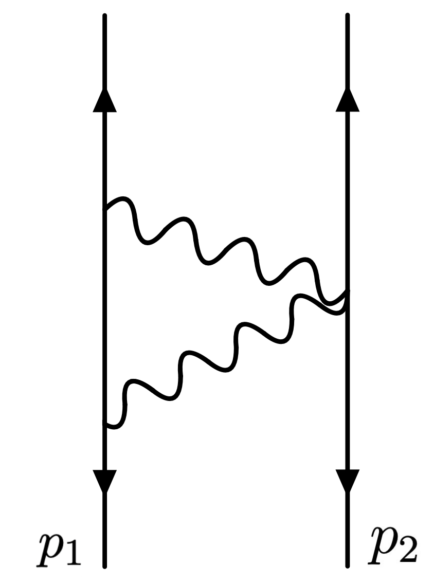
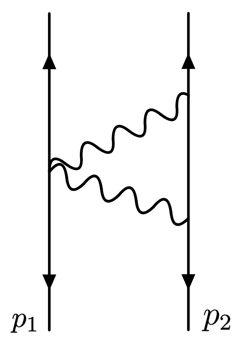
Figure 1: The two diagrams containing classical information for the $2\rightarrow 2$ elastic scattering at 2PM.

We choose as independent loop momentum $l=q_{3}$ and therefore we substitute in (5) $q_{2}=-l-q$ and $\tau_{12}=-t-\tau_{13}$ and $\tau_{22}=t-\tau_{23}$. Taking the classical $t\rightarrow 0$ limit yields,

$$\mathcal{M}^{2\mathrm{PM}}_{\mathrm{even}}(a;p_{i},q)=i\frac{\kappa^{4}}{16}\bigg{[}c_{\triangleright}\mathcal{I}_{\triangleright}(a)+(c_{\triangleright})_{\mu\nu}\mathcal{I}^{\mu\nu}_{\triangleright}(a)+(\triangleright\leftrightarrow\triangleleft)\bigg{]},$$ (5.20)

where,

$$c_{\triangleright}=4m_{1}^{2}[m_{1}^{4}+m_{1}^{2}(m_{2}^{2}-2s)+(m_{2}^{2}-s)^{2}],\qquad(c_{\triangleright})_{\mu\nu}=-\frac{8m_{1}^{4}p_{2\mu}p_{2\nu}}{t},$$ (5.21)

and,

$$\mathcal{I}^{\mu_{1}\dots\mu_{n}}_{\triangleright}(a)=\int\frac{d^{4}l}{(2\pi)^{4}}\frac{l^{\mu_{1}}\dots l^{\mu_{n}}\cosh(2a\cdot l+a\cdot q)}{l^{2}(l+q)^{2}[(p_{1}+l)^{2}-m_{1}^{2}]},$$ (5.22)

and where quantities with $\triangleleft$ can be obtained from $\triangleright$ by sending $m_{1}\leftrightarrow m_{2}$ and $p_{1}\leftrightarrow p_{2}$.

Since we are ultimately interested in obtaining the scattering angle, from now on we consider an aligned spin configuration, where the spins of the black holes are aligned to the $z$ axis and perpendicular to the scattering plane $xy$. We also choose to work in the center of mass frame and we fix,

$$p_{1}=(-E_{1},-p,0,0),\qquad p_{2}=(-E_{2},p,0,0),\qquad a_{i}=(0,0,0,a_{i}).$$ (5.23)

Using (D.10) and (D.15), we find in the classical limit,

$$\mathcal{M}^{2\mathrm{PM}}_{\mathrm{even}}(a;p_{i},q)= \frac{\kappa^{4}}{16}\frac{1}{32\sqrt{-q^{2}}}\bigg{\{}4m_{1}[m_{1}^{4}+m_{1}^{2}(m_{2}^{2}-2s)+(m_{2}^{2}-s)^{2}]I_{0}(\mathscr{F}(a,q))$$

$$+2m_{1}\bigg{[}m_{1}^{2}m_{2}^{2}-\frac{(s-m_{1}^{2}-m_{2}^{2})^{2}}{4}\bigg{]}\frac{I_{1}(\mathscr{F}(a,q))}{\mathscr{F}(a,q)}+(m_{1}\leftrightarrow m_{2})\bigg{\}},$$ (5.24)

where $I_{0}(x)$ and $I_{1}(x)$ are modified Bessel functions of the first kind and their argument is,

$$\mathscr{F}(a,q)=\sqrt{(a\cdot q)^{2}-a^{2}q^{2}},$$ (5.25)

which is shift symmetric. We checked that equation (5) reduces to the standard 2PM result for $a=0$, e.g. [30]. Let us now consider the part of the 2PM amplitude containing odd powers of the classical spin vector. We get,

$$\mathcal{M}^{2\mathrm{PM}}_{\mathrm{odd}}(a;p_{i},q)=\frac{\kappa^{4}}{16}\bigg{[}d_{\triangleright}\epsilon_{\mu}(q,p_{2},p_{1})\mathcal{J}^{\mu}_{\triangleright}(a)+(d_{\triangleright})_{\nu}\epsilon_{\mu}(q,p_{2},p_{1})\mathcal{J}^{\mu\nu}_{\triangleright}(a)+(\triangleright\leftrightarrow\triangleleft)\bigg{]},$$ (5.26)

where,

$$d_{\triangleright}=\frac{8m_{1}^{2}(m_{1}^{2}+m_{2}^{2}-s)}{t},\qquad(d_{\triangleright})_{\nu}=-\frac{16m_{1}^{2}p_{2\nu}}{t},$$ (5.27)

and,

$$\mathcal{J}^{\mu_{1}\dots\mu_{n}}(a)=\int\frac{d^{4}l}{(2\pi)^{4}}\frac{l^{\mu_{1}}\dots l^{\mu_{n}}\sinh(2a\cdot l+a\cdot q)}{l^{2}(l+q)^{2}[(l+p_{1})^{2}-m_{1}^{2}]}.$$ (5.28)

We find that in the classical limit only the vector integral contributes in (5.26) and we have, using (D.26),

$$\mathcal{M}^{2\mathrm{PM}}_{\mathrm{odd}}(a;p_{i},q)= \frac{\kappa^{4}}{16}\bigg{[}\frac{m_{1}(m_{1}^{2}+m_{2}^{2}-s)}{32\sqrt{-q^{2}}}i\epsilon(a,q,p_{2},p_{1})\frac{I_{1}(\mathscr{F}(a,q))}{\mathscr{F}(a,q)}$$

$$+(m_{1}\leftrightarrow m_{2})\bigg{]}.$$ (5.29)

Computing the Gram determinant gives (see (C.5)-(C.6)),

$$\epsilon(a,q,p_{2},p_{1})=i\mathscr{F}(a,q)m_{1}m_{2}\sqrt{\sigma^{2}-1}+\mathcal{O}(t^{2}).$$ (5.30)

Substituting into (5) gives the final result for the classical 2PM amplitude odd in the spin,

$$\mathcal{M}^{2\mathrm{PM}}_{\mathrm{odd}}(a;p_{i},q)= -\frac{\kappa^{4}}{16}\frac{\sqrt{\sigma^{2}-1}}{32\sqrt{-q^{2}}}\bigg{[}m_{1}(m_{1}^{2}+m_{2}^{2}-s)I_{1}(\mathscr{F}(a,q))$$

$$+(m_{1}\leftrightarrow m_{2})\bigg{]},$$ (5.31)

where the Lorentz factor is related to $s$ by $\sigma=\frac{1}{2m_{1}m_{2}}(s-m_{1}^{2}-m_{2}^{2})$.

The 2PM eikonal phase is,

$$\tilde{\mathcal{M}}^{2\mathrm{PM}}(\mathbf{a};p_{i},\mathbf{b}) =\frac{1}{4m_{1}m_{2}\sqrt{\sigma^{2}-1}}\int\frac{d^{2}\mathbf{q}}{(2\pi)^{2}}\mathcal{M}^{2\mathrm{PM}}(\mathbf{a};p_{i},\mathbf{q})e^{-i\mathbf{q}\cdot\mathbf{b}}$$

$$=\tilde{\mathcal{M}}^{2\mathrm{PM}}_{\mathrm{even}}(\mathbf{a};p_{i},\mathbf{b})+\tilde{\mathcal{M}}_{\mathrm{odd}}^{2\mathrm{PM}}(\mathbf{a};p_{i},\mathbf{b}).$$ (5.32)

where,

$$\tilde{\mathcal{M}}^{2\mathrm{PM}}_{\mathrm{even}}(\mathbf{a};p_{i},\mathbf{b})= \frac{\kappa^{4}}{16}\frac{1}{128m_{1}m_{2}\sqrt{\sigma^{2}-1}}\bigg{\{}4m_{1}[m_{1}^{4}+m_{1}^{2}(m_{2}^{2}-2s)+(m_{2}^{2}-s)^{2}]\tilde{I}_{0}[\mathbf{a},\mathbf{b}]$$

$$+2m_{1}\bigg{[}m_{1}^{2}m_{2}^{2}-\frac{(s-m_{1}^{2}-m_{2}^{2})^{2}}{4}\bigg{]}\tilde{\bigg{(}\frac{I_{1}}{\mathscr{F}}\bigg{)}}[\mathbf{a},\mathbf{b}]+(m_{1}\leftrightarrow m_{2})\bigg{\}},$$ (5.33)

and,

$$\tilde{\mathcal{M}}^{2\mathrm{PM}}_{\mathrm{odd}}(\mathbf{a};p_{i},\mathbf{b})= -\frac{\kappa^{4}}{16}\frac{1}{128m_{1}m_{2}}\bigg{[}m_{1}(m_{1}^{2}+m_{2}^{2}-s)\tilde{I}_{1}[\mathbf{a},\mathbf{b}]$$

$$+(m_{1}\leftrightarrow m_{2})\bigg{]},$$ (5.34)

where the Fourier transforms of the Bessel functions are computed in appendix E in (E), (E) and (E). The 2PM scattering angle is defined through the usual relation,

$$\Theta^{2\mathrm{PM}}(a;p,b)=-\frac{1}{p}\frac{\partial}{\partial b}\mathcal{M}^{\mathrm{2PM}}(a;p,b)=\Theta^{2\mathrm{PM}}_{\mathrm{even}}(a;p,b)+\Theta^{2\mathrm{PM}}_{\mathrm{odd}}(a;p,b),$$ (5.35)

where,

$$\Theta^{2\mathrm{PM}}_{\mathrm{even}}(a;p,b)=-\frac{1}{p}\frac{\partial}{\partial b}\mathcal{M}^{\mathrm{2PM}}_{\mathrm{even}}(a;p,b),\qquad\Theta^{2\mathrm{PM}}_{\mathrm{odd}}(a;p,b)=-\frac{1}{p}\frac{\partial}{\partial b}\mathcal{M}^{\mathrm{2PM}}_{\mathrm{odd}}(a;p,b).$$ (5.36)

6 Conclusions and outlook

We introduced a new Yang-Mills type of Lagrangian based on a notion of minimal coupling that incorporates classical spin effects. In particular, we found that the three-point amplitude of $\sqrt{\mathrm{Kerr}}$ can consistently be described using a “classical spin covariant derivative”, whose implementation at the level of the Lagrangian automatically yields contact terms. We used such theory to compute the Compton amplitude to all orders in the spin, first in gauge theory and then, using classical double copy, in gravity. Such amplitudes, coming directly from a local Lagrangian, are not affected by spurious poles and they reproduce the well-known result in the equal-helicity sector whereas they do not in the opposite-helicity one. In particular, we showed that the opposite-helicity Compton amplitude coming from our model does not depend on the complex vector $w$ present e.g. in [92, 123]. We concluded with a 1-loop (2PM) computation of the scattering amplitude for an elastic $2\rightarrow 2$ process in an aligned spin configuration, to all orders in the classical spin vector, from which we extracted the 2PM eikonal and scattering angle.

As remarked above, the field theory constructed here does not capture all the features characterizing $\sqrt{\mathrm{Kerr}}$ and Kerr solutions and their interactions with the gauge fields. However, it has to be regarded as a minimal model to which one is free to add gauge invariant terms of higher order in the curvature in order to reproduce correct amplitudes and observables relevant for the dynamics of true Kerr binaries in the PM regime. The main advantage of this theory relies in its intrinsic simplicity, which we believe to be a fundamental criterion for the description of Kerr black holes as elementary particles. Indeed, the 1PM and the 2PM elastic scattering amplitudes have a very simple mathematical structure. Concerning future directions, it would be interesting to go further in the PM expansion and to explicitly compute the 3PM scattering amplitude and eikonal, both in the conservative and radiative sectors as well as to construct a worldline version of this theory.

Acknowledgements

I would like to thank Maor Ben-Shahar, Zvi Bern, Luca Buoninfante, Paolo Di Vecchia, Alessandro Georgoudis, Kays Haddad, Carlo Heissenberg, Gustav Jakobsen, Henrik Johansson, Gustav Mogull, Stavros Mougiakakos, Alexander Ochirov, Paolo Pichini, Jan Plefka and Justin Vines for very useful discussions. I thank Henrik Johansson and Paolo Pichini for their interest during initial stages of the project. I am especially grateful to Kays Haddad, Henrik Johansson and Paolo Pichini for enlightening discussions and to Paolo Di Vecchia and Paolo Pichini for comments on this draft. The research of FA is fully supported by the Knut and Alice Wallenberg Foundation under grant KAW 2018.0116. Nordita is partially supported by Nordforsk.

Appendix A Kerr-Schild coordinates and Newman-Janis shift

In this appendix we review some features of the Schwarzschild and Kerr solutions using the Kerr-Schild ansatz [74, 136, 142], that consists in parametrizing the full spacetime metric $g_{\mu\nu}$ as,

$$g_{\mu\nu}=\bar{g}_{\mu\nu}+\hskip 1.42271pt\phi\hskip 1.42271ptk_{\mu}k_{\nu},\hskip 28.45274pt\bar{g}_{\mu\nu}{k}^{\mu}k^{\nu}=0=g_{\mu\nu}{k}^{\mu}k^{\nu},$$ (A.1)

where $\bar{g}_{\mu\nu}$ is a background solution satisfying $\bar{R}_{\mu\nu}=0$. Because $k^{\mu}$ is null, its indices can be raised and lowered with both $g_{\mu\nu}$ and $\bar{g}_{\mu\nu}$. Vacuum Einstein equations $R_{\mu\nu}=0$, together with (A.1) imply [71],

$$R^{(1)}_{\mu\nu}\equiv\bar{\nabla}_{\rho}\bigg{(}\bar{\nabla}_{(\mu}(\phi\hskip 1.42271ptk_{\nu)}k^{\rho})-\frac{1}{2}\bar{\nabla}^{\rho}(\phi\hskip 1.42271ptk_{\mu}k_{\nu})\bigg{)}=0.$$ (A.2)

We are interested in describing black holes and hence, from now on we choose $\phi$ to depend only on the radial coordinate $r$ and on the coordinate $z$, i.e. we specialize to axisymmetric solutions. Furthermore, we fix $k^{\mu}=(1,-1,0,0)$ [87] and choose $\bar{g}_{\mu\nu}$ to be the flat Minkowski metric $\eta_{\mu\nu}$.

If we work in spherical coordinates $(r,\theta,\phi)$ defined by $x+iy=re^{i\phi}\sin\theta$ and $z=r\cos\theta$, it is immediate to prove that $R^{(1)}_{\mu\nu}=0$ implies,

$$\phi+r\partial_{r}\phi=0,\hskip 28.45274pt\partial_{r}\partial_{\theta}\phi=0,$$ (A.3)

whose solution is,

$$\phi_{S}=\frac{r_{s}}{r},\hskip 28.45274pt,$$ (A.4)

where $r_{s}=2G_{N}m$, that is precisely the Schwarzschild black hole in Kerr-Schild coordinates.

To obtain the Kerr solution, we perform a change of coordinates and parametrize $\eta_{\mu\nu}$ with oblate spheroidal coordinates, defined by $x+iy=(r+ia)e^{i\phi}\sin\theta$ and $z=r\cos\theta$. Notice that so far, the parameter $a$ is not related to the spin and it appears as mere parameter characterizing the foliation of the spatial part of the spacetime metric. Equation (A.2) reduces to,

$$\frac{r^{2}-a^{2}\cos^{2}\theta}{r^{2}+a^{2}\cos^{2}\theta}\phi+r\partial_{r}\phi=0,\hskip 28.45274pt\partial_{r}\partial_{\theta}\phi-\partial_{r}\bigg{(}\frac{2a^{2}\phi\sin\theta\cos\theta}{r^{2}+a^{2}\cos^{2}\theta}\bigg{)}=0,$$ (A.5)

solved by,

$$\phi_{K}=\frac{r_{s}r}{r^{2}+a^{2}\cos^{2}\theta},$$ (A.6)

which is the Kerr-Schild form of Kerr spacetime. We note here that performing a change of coordinates from spherical to oblate spheroidal on the Schwarzschild solution (A.4) does not yield Kerr. Indeed, the two black holes are not diffeomorphic. Only performing the diffeomorphism on the ansatz for the metric, before solving Einstein equations, gives Kerr spacetime. One of the advantages of using Kerr-Schild coordinates is that they emphasize the similarities between Schwarzschild and Kerr and that there is a simple and clear connection between them called Newman-Janis shift [137]. It consists in temporarily complexifying the radial coordinate of the Schwarzschild solution and then perform the complex translation $r\rightarrow r+ia\cos\theta$ to reconstruct Kerr spacetime as follows:

$$\phi_{K}=\frac{1}{2}(\phi_{S}+\phi_{S}^{*})|_{r\rightarrow r+ia\cos\theta}=\frac{r_{s}}{2}\bigg{(}\frac{1}{r+ia\cos\theta}+\frac{1}{r-ia\cos\theta}\bigg{)}.$$ (A.7)

This equation displays that all the information about the spinning solution are actually encoded into the spinless one. All the curvature invariants constructed with the Kerr metric can be obtained by Newman-Janis shifting the Schwarzschild ones, e.g.

$$R^{S}_{\mu\nu\rho\sigma}R^{\mu\nu\rho\sigma}_{S}=\frac{48G^{2}m^{2}}{r^{6}},$$ (A.8)

and,

$$R^{K}_{\mu\nu\rho\sigma}R^{\mu\nu\rho\sigma}_{K}=24G^{2}m^{2}\frac{2r^{6}-30a^{2}r^{4}\cos^{2}\theta+30a^{4}r^{2}\cos^{4}\theta-2a^{6}\cos^{6}\theta}{(r^{2}+a^{2}\cos^{2}\theta)^{6}},$$ (A.9)

are simply related by,

$$R^{K}_{\mu\nu\rho\sigma}R^{\mu\nu\rho\sigma}_{K}=\frac{1}{2}(R^{S}_{\mu\nu\rho\sigma}R^{\mu\nu\rho\sigma}_{S}+(R^{S}_{\mu\nu\rho\sigma}R^{\mu\nu\rho\sigma}_{S})^{*})|_{r\rightarrow r+ia\cos\theta}.$$ (A.10)

The construction of the field theory described in the paper is based on an implementation of the Newman-Janis shift at the level of the Lagrangian.

We end this section by showing the gauge theory, single copy classical solutions corresponding to Schwarzschild and Kerr, namely Coulomb and $\sqrt{\mathrm{Kerr}}$. We parametrize the gauge field as,

$$A^{\mu}=\phi k^{\mu},\hskip 28.45274pt\eta_{\mu\nu}k^{\mu}k^{\nu}=0.$$ (A.11)

with $k^{\mu}=(1,-1,0,0)$. In spherical and oblate spheroidal coordinates, the solutions to equations of motion $D_{\mu}F^{\mu\nu}=0$ for $\phi$ turn out to be,

$$A^{\mu}_{S}=\phi_{S}k^{\mu},\hskip 28.45274ptA^{\mu}_{K}=\phi_{K}k^{\mu},$$ (A.12)

respectively, where again $\phi_{S}$ and $\phi_{K}$ are given in (A.4) and (A.6) with the replacement $r_{s}\rightarrow g$. As discussed in [3, 72, 73, 71, 87], the classical double copy structure between the gauge theory and gravity solutions is evident.

Appendix B Comparison with other Compton amplitudes

In this appendix we compare the opposite-helicity Compton amplitudes in (3.8) following from the Lagrangian (2.18) with other present in the literature. In order to do so, we specify the kinematics setup as e.g. in [125],

$$p_{1}=-(m,0,0,0),\qquad q_{2}=-\hbar(\omega,0,0,\omega),$$ (B.1)

$$q_{3}=\frac{\hbar\omega}{1+\frac{2\hbar\omega}{m}\sin^{2}(\theta/2)}(1,0,\sin\theta,\cos\theta),\qquad p_{4}=-p_{1}-q_{2}-q_{3},$$ (B.2)

$$\epsilon_{2}^{+}=\frac{1}{\sqrt{2}}(0,1,i,0),\qquad \epsilon_{2}^{-}=-\frac{1}{\sqrt{2}}(0,1,-i,0),$$ (B.3)

$$\epsilon_{3}^{+}=\frac{1}{\sqrt{2}}(0,\cos\theta,i,\sin\theta),\qquad \epsilon_{3}^{-}=-\frac{1}{\sqrt{2}}(0,\cos\theta,-i,\sin\theta),$$ (B.4)

and $a=\frac{1}{\hbar}(0,a^{x},a^{y},a^{z})$ . As explained at the end of section 3, the opposite-helicity sector differs from the one originally presented in [75]. We can parametrize the difference by introducing the complex vectors [92, 123],

$$w=-\frac{\omega(q_{2}-q_{3})+\frac{i}{m\hbar}\epsilon(q_{2},q_{3},p_{1})}{2\omega\cos^{2}(\theta/2)},\qquad w^{*}=-\frac{\omega(q_{2}-q_{3})-\frac{i}{m\hbar}\epsilon(q_{2},q_{3},p_{1})}{2\omega\cos^{2}(\theta/2)},$$ (B.5)

and therefore, by denoting by $\tilde{\mathcal{A}}^{\pm\mp}_{4}(a)$ the opposite-helicity Compton amplitudes shown in [125] for $s<2$, their relation to the ones in (3.9) is,

$$\tilde{\mathcal{A}}^{+-}_{4}(a;p_{i},q_{i})=e^{-2a\cdot w}\mathcal{A}_{4}^{+-}(a;p_{i},q_{i}),\qquad\tilde{\mathcal{A}}^{-+}_{4}(a;p_{i},q_{i})=e^{2a\cdot w^{*}}\mathcal{A}_{4}^{+-}(a;p_{i},q_{i}).$$ (B.6)

Indeed, the functions $\tilde{\mathcal{F}}_{+-}(\omega,a,\theta)=\mathcal{F}(\omega,a,\theta)-2a\cdot w$ and $\tilde{\mathcal{F}}_{-+}(\omega,a,\theta)=-\mathcal{F}(\omega,a,\theta)+2a\cdot w^{*}$ are,

$$\tilde{\mathcal{F}}_{+-}(\omega,a,\theta)=\omega(a^{x}+a^{z}\sin\theta+2ia^{y}-a^{x}\cos\theta)\tan(\theta/2),$$ (B.7)

$$\tilde{\mathcal{F}}_{-+}(\omega,a,\theta)=-\omega(a^{x}+a^{z}\sin\theta-2ia^{y}-a^{x}\cos\theta)\tan(\theta/2)=\tilde{\mathcal{F}}^{*}_{+-}(-\omega,a,\theta),$$ (B.8)

and they match the ones in [125].

Let us further analyse the mismatch by looking explicitly at the first order in the spin. Using equation (2.23) and (3) it is simple to show that,

$$\mathcal{A}_{4}(a;p_{i},q_{i})=-\frac{e^{2}}{p_{1}\cdot q_{2}\hskip 1.42271ptp_{1}\cdot q_{3}}[\omega_{0}+\omega_{1}+\mathcal{O}(a^{2})],$$ (B.9)

where,

$$\omega_{0} =2p_{1}\cdot F_{2}\cdot F_{3}\cdot p_{1},$$ (B.10)

$$\omega_{1} =-i(p_{1}\cdot F_{3}\cdot q_{2}F_{2\mu\nu}+p_{1}\cdot F_{2}\cdot q_{3}F_{3\mu\nu})S^{\mu\nu}$$

$$\hskip 14.22636pt+2(p_{1}\cdot q_{3}F_{3}\cdot F_{2}^{*}\cdot a+p_{1}\cdot q_{2}F_{2}\cdot F_{3}^{*}\cdot a)\equiv\omega_{11}+\omega_{12}.$$ (B.11)

If we denote by $\tilde{\omega}_{1}$ the coefficient linear in the spin in (E.3) of [125], the difference with respect to (B.11) is,

$$\Delta\omega_{1}=\omega_{1}-\tilde{\omega}_{1}= \hskip 0.28436pt(p_{1}\cdot q_{3}F_{3}\cdot F_{2}^{*}\cdot a+p_{1}\cdot q_{2}F_{2}\cdot F_{3}^{*}\cdot a)$$

$$-i\frac{p_{1}\cdot(q_{2}-q_{3})}{2}(F_{2}^{\mu}{}_{\rho}F_{3}^{\rho\nu}-F_{3}^{\mu}{}_{\rho}F_{2}^{\rho\nu})S_{\mu\nu}.$$ (B.12)

Quite interestingly, $\Delta\omega_{1}$ is exactly vanishing when plugging polarization vectors having the same helicity as it should, for the equal-helicity sector result following from our model is correct. However, when the two helicities are opposite $\Delta\omega_{1}$ is not zero. In particular, the term in the last line of (B) vanishes for opposite helicities, whereas the second term in (B.11) does not. Consequently, using the relations in (B.6), we get

$$\frac{\omega_{11}^{+-}}{p_{1}\cdot F_{2}^{+}\cdot F_{3}^{-}\cdot p_{1}}=-a\cdot(q_{2}-q_{3})-2a\cdot w,\qquad\frac{\omega_{12}^{+-}}{p_{1}\cdot F_{2}^{+}\cdot F_{3}^{-}\cdot p_{1}}=2a\cdot w,$$ (B.13)

$$\frac{\omega_{11}^{-+}}{p_{1}\cdot F_{2}^{-}\cdot F_{3}^{+}\cdot p_{1}}=a\cdot(q_{2}-q_{3})+2a\cdot w^{*},\qquad\frac{\omega_{12}^{-+}}{p_{1}\cdot F_{2}^{-}\cdot F_{3}^{+}\cdot p_{1}}=-2a\cdot w^{*},$$ (B.14)

in the classical limit.

Appendix C 1PM amplitude for $\sqrt{\mathrm{Kerr}}$

The 1PM amplitude between two $\sqrt{\mathrm{Kerr}}$ particles having charges $e_{1}$ and $e_{2}$ exchanging one photon with momentum $q$ can be obtained by gluing together two three-point amplitudes with the Feynman propagator, as shown in (C.1),

$$i\mathcal{A}^{1\mathrm{PM}}(a;p_{i},q)=\vbox{\hbox{\includegraphics[width=128.0374pt,height=125.19194pt]{1PM.png}}},$$ (C.1)

because in the classical limit only the $t=q^{2}$ pole contributes. Before doing so, we use three-point kinematics to rewrite $\mathcal{A}^{\mu}_{3}(a,p)$ in a more convenient form,

$$\mathcal{A}^{\mu}_{3}(a;p,q) =-ie\hskip 0.85355pt\mathrm{exp}\{i\epsilon^{\mu}{}_{\rho}(a,q)\}p^{\rho}$$

$$=-ie\left(p^{\mu}\cosh(a\cdot q)+i\frac{\epsilon^{\mu}(p,a,q)}{a\cdot q}\sinh(a\cdot q)\right).$$ (C.2)

Therefore, the 1PM amplitude is given by,

$$i\mathcal{A}^{1\mathrm{PM}}(a;p_{i},q)= -\frac{i}{q^{2}}\eta_{\mu\nu}\mathcal{A}_{3}^{\mu}(a_{1};p_{1},q)\mathcal{A}^{\nu}_{3}(a_{2},p_{2},-q)$$

$$= \frac{i}{q^{2}}e_{1}e_{2}\bigg{(}p_{1}\cdot p_{2}\cosh(a_{1}\cdot q)\cosh(a_{2}\cdot q)$$

$$+\epsilon^{\mu}(p_{1},a_{1},q)\epsilon_{\mu}(p_{2},a_{2},q)\frac{\sinh(a_{1}\cdot q)\sinh(a_{2}\cdot q)}{a_{1}\cdot qa_{2}\cdot q}$$

$$+i\epsilon(p_{2},p_{1},a_{1},q)\cosh(a_{2}\cdot q)\frac{\sinh(a_{1}\cdot q)}{a_{1}\cdot q}$$

$$-i\epsilon(p_{1},p_{2},a_{2},q)\cosh(a_{1}\cdot q)\frac{\sinh(a_{2}\cdot q)}{a_{2}\cdot q}\bigg{)}.$$ (C.3)

Using $q\cdot p_{1}=0=q\cdot p_{2}$ and $p_{1}\cdot a_{1}=0=p_{2}\cdot a_{2}$, together with $q^{2}=0$, we compute the following Gram determinants [86],

$$\epsilon^{\mu}(p_{1},a_{1},q)\epsilon_{\mu}(p_{2},a_{2},q)=m_{1}m_{2}\sigma a_{1}\cdot qa_{2}\cdot q,$$ (C.4)

$$\epsilon(p_{1},p_{2},a_{1},q)=im_{1}m_{2}(a_{1}\cdot q)\sqrt{\sigma^{2}-1},$$ (C.5)

$$\epsilon(p_{1},p_{2},a_{2},q)=im_{1}m_{2}(a_{2}\cdot q)\sqrt{\sigma^{2}-1},$$ (C.6)

where $\sigma=\frac{p_{1}\cdot p_{2}}{m_{1}m_{2}}$ is the Lorentz factor. Substituting the above relations back into (C) we get,

$$i\mathcal{A}^{1\mathrm{PM}}(a;p_{i},q)= \frac{ie_{1}e_{2}m_{1}m_{2}}{q^{2}}\bigg{\{}\sigma\bigg{[}\cosh\left(a_{1}\cdot q\right)\cosh\left(a_{2}\cdot q\right)+\sinh\left(a_{1}\cdot q\right)\sinh\left(a_{2}\cdot q\right)\bigg{]}$$

$$+\sqrt{\sigma^{2}-1}\bigg{[}\cosh\left(a_{2}\cdot q\right)\sinh\left(a_{1}\cdot q\right)+\cosh\left(a_{1}\cdot q\right)\sinh\left(a_{2}\cdot q\right)\bigg{]}\bigg{\}}$$

$$= \frac{ie_{1}e_{2}m_{1}m_{2}}{q^{2}}\bigg{[}\sigma\cosh(a\cdot q)+\sqrt{\sigma^{2}-1}\sinh(a\cdot q)\bigg{]},$$ (C.7)

where $a=a_{1}+a_{2}$. Introducing the relative velocity of the two bodies $v=\frac{\sqrt{\sigma^{2}-1}}{\sigma}$ we get for the classical 1PM amplitude,

$$\mathcal{A}^{1\mathrm{PM}}(a;p_{i},q)=\frac{e_{1}m_{1}e_{2}m_{2}}{2q^{2}}\sigma\sum_{\pm}(1\pm v)e^{\pm i\frac{\epsilon(p_{1},p_{2},q,a)}{m_{1}m_{2}\sigma v}},$$ (C.8)

compatibly with [87], where we inverted (C.5) and (C.6) to get $a\cdot q=i\frac{\epsilon(p_{1},p_{2},q,a)}{m_{1}m_{2}\sigma v}$.

It is instructive to show how to get the 1PM amplitude also by summing over the helicities of intermediate polarizations,

$$i\mathcal{A}^{\mathrm{1PM}}(a;p_{i},q_{i})=-\frac{i}{q^{2}}\sum_{h=\pm}\mathcal{A}_{3}^{\mu}(a_{1};p_{1},q)\epsilon^{h}_{\mu}(q)\epsilon^{-h}_{\nu}(-q)\mathcal{A}_{3}^{\nu}(a_{2};p_{2},-q).$$ (C.9)

Using now the definition of $\epsilon^{\prime\mu}$, the previous equation becomes,

$$i\mathcal{A}^{\mathrm{1PM}}(a;p_{i},q_{i})=-\frac{i}{q^{2}}\sum_{h=\pm}\mathcal{A}_{3}^{\mu}(p_{1},q)\epsilon^{\prime h}_{\mu}(a_{1},q)\epsilon^{\prime-h}_{\nu}(a_{2},-q)\mathcal{A}_{3}^{\nu}(p_{2},-q).$$ (C.10)

We introduce projectors onto positive and negative helicity states,

$$\Pi^{+}_{\mu\nu}(q)=\epsilon_{\mu}^{+}(q)\epsilon_{\nu}^{-}(-q)=\frac{1}{2}\eta_{\mu\nu}+\frac{1}{2}\frac{q_{\mu}k_{\nu}+q_{\nu}k_{\mu}}{q\cdot k}+\frac{i}{2}\frac{\epsilon_{\mu\nu}(q,k)}{q\cdot k},$$ (C.11)

$$\Pi^{-}_{\mu\nu}(q)=\epsilon_{\mu}^{-}(q)\epsilon_{\nu}^{+}(-q)=\frac{1}{2}\eta_{\mu\nu}+\frac{1}{2}\frac{q_{\mu}k_{\nu}+q_{\nu}k_{\mu}}{q\cdot k}-\frac{i}{2}\frac{\epsilon_{\mu\nu}(q,k)}{q\cdot k},$$ (C.12)

where $k$ is an arbitrary reference null vector. They satisfy,

$$\Pi^{\pm}_{\mu}{}^{\rho}(q)\Pi_{\rho}^{\pm}{}^{\nu}(q)=\Pi_{\mu}^{\pm}{}^{\nu}(q),\qquad\Pi^{\pm}_{\mu}{}^{\rho}(q)\Pi_{\rho}^{\mp}{}^{\nu}(q)=0,$$ (C.13)

$$\Pi^{+}_{\mu\nu}(q)+\Pi^{-}_{\mu\nu}(q)=\eta_{\mu\nu}+\frac{q_{\mu}k_{\nu}+q_{\nu}k_{\mu}}{q\cdot k}=\Pi_{\mu\nu}(q),\qquad\Pi_{\mu}{}^{\rho}(q)\Pi_{\rho}{}^{\nu}(q)=\Pi_{\mu}{}^{\nu}(q).$$ (C.14)

Up to gauge transformations $\epsilon^{\prime\mu}_{h}=e^{-ha\cdot q}\epsilon^{\mu}_{h}$ and hence the sum appearing in (C.10) reads,

$$\sum_{h=\pm}e^{-ha_{1}\cdot q}\epsilon^{h}_{\mu}(q)e^{ha_{2}\cdot q}\epsilon^{h}_{\nu}(-q)= \bigg{(}\eta_{\mu\nu}-\frac{q_{\mu}k_{\nu}+q_{\nu}k_{\mu}}{q\cdot k}\bigg{)}\cosh(a\cdot q)$$

$$-i\frac{\epsilon_{\mu\nu}(q,k)}{q\cdot k}\sinh(a\cdot q)\equiv\Pi_{\mu\nu}(a;q),$$ (C.15)

where $a=a_{1}+a_{2}$. $\Pi_{\mu\nu}(a)$ is a spin-dressed projector and it satisfies,

$$\Pi_{\mu}{}^{\rho}(a;q)\Pi_{\rho}{}^{\nu}(b;q)=\Pi_{\mu}{}^{\nu}(a+b;q).$$ (C.16)

The 1PM amplitude in (C.9) can be written in terms of $\Pi_{\mu}{}^{\nu}(a;q)$ as,

$$i\mathcal{A}^{1\mathrm{PM}}(a;p_{i},q_{i})=-\frac{i}{q^{2}}\mathcal{A}_{3}^{\mu}(p_{1},q)\Pi_{\mu\nu}(a;q)\mathcal{A}_{3}^{\nu}(p_{2},-q).$$ (C.17)

This equation shows that the full dependence on the classical spin of the 1PM amplitude is actually encoded into a suitable “spin dressing” of the Feynman propagator.

Similarly, the gravity 1PM amplitude in (4.11) can be written as,

$$i\mathcal{M}^{1\mathrm{PM}}(a;p_{i},q_{i}) =-\frac{i}{q^{2}}\mathcal{M}_{3}^{\mu\nu}(a_{1};p_{1},q)\Pi_{\mu\nu;\rho\sigma}(q)\mathcal{M}_{3}^{\rho\sigma}(a_{2};p_{2},-q)$$

$$=-\frac{i}{q^{2}}\mathcal{M}_{3}^{\mu\nu}(p_{1},q)\Pi_{\mu\nu;\rho\sigma}(a;q)\mathcal{M}_{3}^{\rho\sigma}(p_{2},-q),$$ (C.18)

where $\Pi_{\mu\nu;\rho\sigma}(a;q)$ is a spin-dressed de Donder projector,

$$\Pi_{\mu\nu;\rho\sigma}(a;q)= \frac{1}{2}\bigg{[}\Pi_{\mu\rho}(a;q)\Pi_{\nu\sigma}(a;q)+\Pi_{\mu\sigma}(a;q)\Pi_{\nu\rho}(a;q)-\Pi_{\mu\nu}(a;q)\Pi_{\rho\sigma}(a;q)\bigg{]}$$

$$= \frac{1}{2}\bigg{[}\Pi_{\mu\rho}(q)\Pi_{\nu\sigma}(q)+\Pi_{\mu\sigma}(q)\Pi_{\nu\rho}(q)-\Pi_{\mu\nu}(q)\Pi_{\rho\sigma}(q)\bigg{]}\cosh(a\cdot q)$$ (C.19)

$$-\frac{i}{2q\cdot k}\bigg{[}\epsilon_{\nu\sigma}(q,k)\Pi_{\mu\rho}(q)+\epsilon_{\mu\rho}(q,k)\Pi_{\nu\sigma}(q)\bigg{]}\sinh(a\cdot q).$$

satisfying,

$$\Pi_{\mu\nu}{}^{\alpha\beta}(a;q)\Pi_{\alpha\beta}{}^{\rho\sigma}(b;q)=\Pi_{\mu\nu}{}^{\rho\sigma}(a+b;q).$$ (C.20)

Appendix D One-loop integrals

For the 2PM amplitude, we need to solve the integral $\mathcal{I}^{\mu_{1}\dots\mu_{n}}_{\triangleright}(a)$ in (5.22), and hence we start by considering the family of integrals,

$$\mathcal{I}^{\mu_{1}\dots\mu_{n}}_{\triangleright}(0)=\int\frac{d^{4}l}{(2\pi)^{4}}\frac{l^{\mu_{1}}\dots l^{\mu_{n}}}{l^{2}(l+q)^{2}[(p_{1}+l)^{2}-m_{1}^{2}]}.$$ (D.1)

We find,

$$\mathcal{I}_{\triangleright}(0)=-\frac{i}{32m_{1}\sqrt{-q^{2}}}+\dots,$$ (D.2)

and using the Passarino-Veltmano reduction [143, 144, 145, 146],

$$\mathcal{I}^{\mu}_{\triangleright}(0)=-\frac{i}{32m_{1}\sqrt{-q^{2}}}\bigg{[}-\frac{1}{2}q^{\mu}+\frac{1}{4}\frac{q^{2}}{m_{1}^{2}}p_{1}^{\mu}+\dots\bigg{]},$$ (D.3)

$$\mathcal{I}^{\mu\nu}_{\triangleright}(0)=-\frac{i}{32m_{1}\sqrt{-q^{2}}}\bigg{[}\frac{3}{8}q^{\mu}q^{\nu}+\frac{1}{8}\frac{q^{2}}{m_{1}^{2}}p^{\mu}_{1}p_{1}^{\nu}-\frac{3}{8}\frac{q^{2}}{m_{1}^{2}}p_{1}^{(\mu}q^{\nu)}-\frac{1}{8}q^{2}\eta^{\mu\nu}+\dots\bigg{]},$$ (D.4)

$$\mathcal{I}^{\mu\nu\rho}_{\triangleright}(0)=-\frac{i}{32m_{1}\sqrt{-q^{2}}}\bigg{[}-\frac{5}{16}q^{\mu}q^{\nu}q^{\rho}+\frac{3}{16}\frac{q^{4}}{m_{1}^{4}}p^{\mu}_{1}p_{1}^{\nu}p_{1}^{\rho}-\frac{3}{16}\frac{q^{2}}{m_{1}^{2}}q^{(\mu}p^{\rho}_{1}p^{\nu)}_{1}$$

$$\hskip 85.35826pt+\frac{15}{32}\frac{q^{2}}{m_{1}^{2}}q^{(\mu}q^{\nu}p_{1}^{\rho)}+\frac{3}{16}q^{2}\eta^{(\mu\nu}q^{\rho)}-\frac{3}{16}\frac{q^{2}}{m_{1}^{2}}\eta^{(\mu\nu}p_{1}^{\rho)}+\dots\bigg{]},$$ (D.5)

where $\dots$ denote subleading terms in the classical limit. Expanding in powers of the total spin vector $a^{\mu}$ the integral $\mathcal{I}^{\mu_{1}\dots\mu_{n}}_{\triangleright}(a)$, we see that we need to compute the contractions of the above tensors with $a_{\mu_{1}}\dots a_{\mu_{n}}$. With the aligned spin and the kinematics specified in (5.23), all the scalar products $a\cdot p_{i}$ vanish. Hence, we are only interested in keeping the terms in (D.3)-(D) having products of $q$’s and $\eta$’s. For the latter there is a general formula [147],

$$\mathcal{I}^{\mu_{1}\dots\mu_{n}}(0)= -\frac{i}{32m_{1}\pi^{\frac{3}{2}}\sqrt{-q^{2}}}\sum_{m=0}^{\left[\frac{n}{2}\right]}\frac{(-1)^{n}\Gamma(\frac{1}{2}-m)\Gamma(n-m+\frac{1}{2})\Gamma(m+\frac{1}{2})}{\Gamma(n+1)}\left(\frac{q^{2}}{2}\right)^{m}$$

$$\{[\eta]^{m}[q]^{n-2m}\}^{\mu_{1}\dots\mu_{n}},$$ (D.6)

in the classical limit, where the symbol $\{[\eta]^{m}[q]^{n-2m}\}^{\mu_{1}\dots\mu_{n}}$ comprises all the symmetric structures one can construct with $q$ and $\eta$ having $n$ covariant indices, e.g.

$$\{[\eta]^{0}[q]^{1}\}^{\mu_{1}}=q^{\mu_{1}},$$

$$\{[\eta]^{1}[q]^{0}\}^{\mu_{1}\mu_{2}}=\eta^{\mu_{1}\mu_{2}},$$

$$\{[\eta]^{1}[q]^{1}\}^{\mu_{1}\mu_{2}\mu_{3}}=\eta^{\mu_{1}\mu_{2}}q^{\mu_{3}}+\eta^{\mu_{3}\mu_{1}}q^{\mu_{2}}+\eta^{\mu_{2}\mu_{3}}q^{\mu_{1}}.$$

We have, expanding $\cosh(x)$,

$$\mathcal{I}_{\triangleright}(a)= \sum_{n=0}^{\infty}\frac{1}{(2n)!}\int\frac{d^{4}l}{2\pi)^{4}}\frac{(2a\cdot l+a\cdot q)^{2n}}{l^{2}(l+q)^{2}[(p_{1}+l)^{2}-m_{1}^{2}]}$$

$$= \sum_{n=0}^{\infty}\sum_{k=0}^{2n}\frac{(a\cdot q)^{k}2^{2n-k}}{(2n-k)!k!}a_{\mu_{1}}\dots a_{\mu_{2n-k}}\int\frac{d^{4}l}{(2\pi)^{4}}\frac{l^{\mu_{1}}\dots l^{\mu_{2n-k}}}{l^{2}(l+q)^{2}[(p_{1}+l)^{2}-m_{1}^{2}]}$$

$$= -\frac{i}{32m_{1}\pi^{\frac{3}{2}}\sqrt{-q^{2}}}\sum_{n=0}^{\infty}\sum_{k=0}^{2n}\sum_{m=0}^{[n-\frac{k}{2}]}\frac{(-1)^{k}2^{2n-k}}{(2n-k)!k!}\frac{\Gamma(\frac{1}{2}-m)\Gamma(2n-k+\frac{1}{2})\Gamma(m+\frac{1}{2})}{\Gamma(2n-k+1)}$$

$$\left(\frac{q^{2}a^{2}}{2}\right)^{m}(a\cdot q)^{2n-2m}\frac{(2n-k)!}{m!(2n-k-2m)!2^{m}},$$ (D.7)

where we used that,

$$a_{\mu_{1}}\dots a_{\mu_{n}}\{[\eta]^{m}[q]^{n-2m}\}^{\mu_{1}\dots\mu_{n}}=a^{2m}(a\cdot q)^{n-2m}\frac{n!}{m!(n-2m)!2^{m}}.$$ (D.8)

For $n=0,1,2$ the sum in (D) gives,

$$-\frac{i}{32m_{1}\sqrt{-q^{2}}},\qquad-\frac{i[(a\cdot q)^{2}-a^{2}q^{2}]}{128m_{1}\sqrt{-q^{2}}},\qquad-\frac{i[(a\cdot q)^{2}-a^{2}q^{2}]^{2}}{2048m_{1}\sqrt{-q^{2}}}.$$ (D.9)

These quantities are related to the series expansion of the modified Bessel function of the first kind $I_{0}(\sqrt{(a\cdot q)^{2}-a^{2}q^{2}})$ and, in particular we have,

$$\mathcal{I}_{\triangleright}(a)=\int\frac{d^{4}l}{(2\pi)^{4}}\frac{\cosh(2a\cdot l+a\cdot q)}{l^{2}(l+q)^{2}[(p_{1}+l)^{2}-m_{1}^{2}]}=-\frac{i}{32m_{1}\sqrt{-q^{2}}}I_{0}(\mathscr{F}(a,q)),$$ (D.10)

where we introduced for convenience,

$$\mathscr{F}(a,q)=\sqrt{(a\cdot q)^{2}-a^{2}q^{2}},$$ (D.11)

in the aligned spin case, which is shift-symmetric [110]. We could also derive,

$$a_{\mu}\mathcal{I}^{\mu}_{\triangleright}(a)=\frac{i}{32m_{1}\sqrt{-q^{2}}}\frac{(a\cdot q)}{2}I_{0}(\mathscr{F}(a,q)),$$ (D.12)

$$a_{\mu}a_{\nu}\mathcal{I}^{\mu\nu}_{\triangleright}(a)=-\frac{i}{32m_{1}\sqrt{-q^{2}}}\frac{1}{4}\bigg{\{}[\mathscr{F}^{2}(a,q)+(a\cdot q)^{2}]I_{0}(\mathscr{F}(a,q))$$

$$\hskip 66.86414pt-\mathscr{F}(a,q)I_{1}(\mathscr{F}(a,q))\bigg{\}}.$$ (D.13)

Using the above results, it is simple to show that the Passarino-Veltman decomposition generalizes also to the case of integrals of the form (5.22) and, in particular, we find,

$$\mathcal{I}_{\triangleright}^{\mu}(a)=-\frac{i}{32m_{1}\sqrt{-q^{2}}}\bigg{(}-\frac{1}{2}q^{\mu}+\frac{1}{4}\frac{q^{2}}{m_{1}^{2}}p_{1}^{\mu}-\frac{1}{8}\frac{q^{4}}{m_{1}^{2}}\frac{a\cdot q}{\mathscr{F}(a,q)^{2}}a^{\mu}\bigg{)}I_{0}(\mathscr{F}(a,q)),$$ (D.14)

$$\mathcal{I}_{\triangleright}^{\mu\nu}(a)=Aq^{\mu}q^{\nu}+Bq^{(\mu}p_{1}^{\nu)}+Cp_{1}^{\mu}p_{1}^{\nu}+D\eta^{\mu\nu}+Ea^{\mu}a^{\nu}+Fa^{(\mu}q^{\nu)}+Ga^{(\mu}p_{1}^{\nu)},$$ (D.15)

where,

$$A= -\frac{i}{128m_{1}\sqrt{-q^{2}}}\bigg{[}\frac{2(a\cdot q)^{2}-a^{2}q^{2}}{\mathscr{F}^{2}(a,q)}I_{0}(\mathscr{F}(a,q))-\frac{(a\cdot q)^{2}+a^{2}q^{2}}{\mathscr{F}(a,q)^{3}}I_{1}(\mathscr{F}(a,q))\bigg{]},$$ (D.16)

$$B= \frac{i}{128m_{1}\sqrt{-q^{2}}}\frac{q^{2}}{m_{1}^{2}}\bigg{[}\frac{2(a\cdot q)^{2}-a^{2}q^{2}}{\mathscr{F}(a,q)^{2}}I_{0}(\mathscr{F}(a,q))-\frac{(a\cdot q)^{2}+a^{2}q^{2}}{\mathscr{F}(a,q)^{3}}I_{1}(\mathscr{F}(a,q)\bigg{]},$$ (D.17)

$$C= -\frac{i}{128m_{1}\sqrt{-q^{2}}}\frac{q^{2}}{m_{1}^{2}}\bigg{[}\frac{q^{2}}{2m_{1}^{2}}\frac{2(a\cdot q)^{2}-a^{2}q^{2}}{\mathscr{F}(a,q)^{2}}I_{0}(\mathscr{F}(a,q))+\frac{I_{1}(\mathscr{F}(a,q))}{\mathscr{F}(a,q)}\bigg{]},$$ (D.18)

$$D= \frac{i}{128m_{1}\sqrt{-q^{2}}}q^{2}\bigg{[}\frac{q^{2}}{4m_{1}^{2}}\frac{2(a\cdot q)^{2}-a^{2}q^{2}}{\mathscr{F}(a,q)^{2}}I_{0}(\mathscr{F}(a,q))+\frac{I_{1}(\mathscr{F}(a,q))}{\mathscr{F}(a,q)}\bigg{]},$$ (D.19)

$$E= -\frac{i}{64m_{1}\sqrt{-q^{2}}}q^{4}\bigg{[}\frac{I_{0}(\mathscr{F}(a,q))}{2\mathscr{F}(a,q)^{2}}-\frac{I_{1}(\mathscr{F}(a,q))}{\mathscr{F}(a,q)^{3}}\bigg{]},$$ (D.20)

$$F= \frac{i}{32m_{1}\sqrt{-q^{2}}}q^{2}(a\cdot q)\bigg{[}\frac{I_{0}(\mathscr{F}(a,q))}{2\mathscr{F}(a,q)^{2}}-\frac{I_{1}(\mathscr{F}(a,q))}{\mathscr{F}(a,q)^{3}}\bigg{]},$$ (D.21)

$$G= -\frac{i}{64m_{1}\sqrt{-q^{2}}}\frac{q^{4}(a\cdot q)}{m_{1}^{2}}\bigg{[}\frac{I_{0}(\mathscr{F}(a,q))}{2\mathscr{F}(a,q)^{2}}-\frac{I_{1}(\mathscr{F}(a,q))}{\mathscr{F}(a,q)^{3}}\bigg{]}.$$ (D.22)

Using similar arguments we find,

$$\mathcal{J}_{\triangleright}(a)=\int\frac{d^{4}l}{(2\pi)^{4}}\frac{\sinh(2a\cdot l+a\cdot q)}{l^{2}(l+q)^{2}[(p_{1}+l)^{2}-m_{1}^{2}]}=0,$$ (D.23)

and,

$$a_{\mu}\mathcal{J}^{\mu}_{\triangleright}(a)=-\frac{i}{64m_{1}\sqrt{-q^{2}}}\mathscr{F}(a,q)I_{1}(\mathscr{F}(a,q)),$$ (D.24)

$$a_{\mu}a_{\nu}\mathcal{J}_{\triangleright}^{\mu}(a)=\frac{i}{64m_{1}\sqrt{-q^{2}}}(a\cdot q)\mathscr{F}(a,q)I_{1}(\mathscr{F}(a,q)).$$ (D.25)

The Passarino-Veltman decomposition now is,

$$\mathcal{J}^{\mu}_{\triangleright}(a)=-\frac{i}{64m_{1}\sqrt{-q^{2}}}\bigg{[}(a\cdot q)q^{\mu}-\frac{q^{2}(a\cdot q)}{2m_{1}^{2}}p_{1}^{\mu}-\frac{q^{2}}{2}a^{\mu}\bigg{]}\frac{I_{1}(\mathscr{F}(a,q))}{\mathscr{F}(a,q)},$$ (D.26)

$$\mathcal{J}^{\mu\nu}_{\triangleright}(a)=Aq^{\mu}q^{\nu}+Bq^{(\mu}p_{1}^{\nu)}+Cp_{1}^{\mu}p_{1}^{\nu}+D\eta^{\mu\nu}+Ea^{\mu}a^{\nu}+Fa^{(\mu}q^{\nu)}+Ga^{(\mu}p_{1}^{\nu)},$$ (D.27)

with,

$$A=\frac{i(a\cdot q)}{64m_{1}\sqrt{-q^{2}}}\frac{I_{1}(\mathscr{F}(a,q))}{\mathscr{F}(a,q)},$$ (D.28)

$$B=-\frac{i(a\cdot q)}{64m_{1}\sqrt{-q^{2}}}\frac{q^{2}}{m_{1}^{2}}\frac{I_{1}(\mathscr{F}(a,q))}{\mathscr{F}(a,q)},$$ (D.29)

$$C=\frac{i(a\cdot q)}{64m_{1}\sqrt{-q^{2}}}\frac{2q^{4}}{m_{1}^{4}}\frac{I_{1}(\mathscr{F}(a,q))}{\mathscr{F}(a,q)},$$ (D.30)

$$D=-\frac{i(a\cdot q)}{64m_{1}\sqrt{-q^{2}}}\frac{q^{4}}{4m_{1}^{2}}\frac{I_{1}(\mathscr{F}(a,q))}{\mathscr{F}(a,q)},$$ (D.31)

$$E=-\frac{i(a\cdot q)}{64m_{1}\sqrt{-q^{2}}}\frac{q^{6}}{2m_{1}^{2}}\frac{I_{1}(\mathscr{F}(a,q))}{\mathscr{F}(a,q)^{3}},$$ (D.32)

$$F=-\frac{i}{64m_{1}\sqrt{-q^{2}}}q^{2}\frac{I_{1}(\mathscr{F}(a,q))}{\mathscr{F}(a,q)},$$ (D.33)

$$G=\frac{i}{64m_{1}\sqrt{-q^{2}}}\frac{q^{4}}{2m_{1}^{2}}\frac{I_{1}(\mathscr{F}(a,q))}{\mathscr{F}(a,q)}.$$ (D.34)

We stress again here that the results for the various integrals above are valid only if $a\cdot p_{1}=0$. Furthermore, it is straightforward to prove the following relations,

$$\frac{\partial\mathcal{I}_{\triangleright}(a)}{\partial a_{\mu}}=2\mathcal{J}^{\mu}_{\triangleright}(a)+q^{\mu}\mathcal{J}_{\triangleright}(a),$$ (D.35)

$$\frac{\partial^{2}\mathcal{I}_{\triangleright}(a)}{\partial a_{\mu}\partial a_{\nu}}=4\mathcal{I}_{\triangleright}^{\mu\nu}(a)+2q^{\mu}\mathcal{I}_{\triangleright}^{\nu}(a)+2q^{\nu}\mathcal{I}^{\mu}_{\triangleright}(a)+q^{\mu}q^{\nu}\mathcal{I}_{\triangleright}(a),$$ (D.36)

$$\frac{\partial\mathcal{J}_{\triangleright}(a)}{\partial a_{\mu}}=2\mathcal{I}^{\mu}_{\triangleright}(a)+q^{\mu}\mathcal{I}_{\triangleright}(a),$$ (D.37)

$$\frac{\partial^{2}\mathcal{J}_{\triangleright}(a)}{\partial a_{\mu}\partial a_{\nu}}=4\mathcal{J}_{\triangleright}^{\mu\nu}(a)+2q^{\mu}\mathcal{J}_{\triangleright}^{\nu}(a)+2q^{\nu}\mathcal{J}^{\mu}_{\triangleright}(a)+q^{\mu}q^{\nu}\mathcal{J}_{\triangleright}(a),$$ (D.38)

that are compatible with what we have found so far.

Appendix E 2PM eikonal phase integrals

In order to compute the 2PM eikonal, we need to evaluate the integral,

$$\mathcal{I}_{n}[\mathbf{a};\alpha]\equiv\int\frac{d^{2}\mathbf{q}}{(2\pi)^{2}}\frac{(\mathbf{a}\cdot\mathbf{q})^{n}}{(\mathbf{q}^{2})^{\alpha}}e^{-i\mathbf{q}\cdot\mathbf{b}}=i^{n}a^{i_{1}}\dots a^{i_{n}}\frac{\Gamma(1-\alpha)}{2^{2\alpha}\pi\Gamma(\alpha)}\frac{\partial^{n}}{\partial b^{i_{1}}\dots\partial b^{i_{n}}}(\mathbf{b}^{2})^{\alpha-1}.$$ (E.1)

Using,

$$\frac{\partial^{n}}{\partial b^{i_{1}}\dots\partial b^{i_{n}}}(\mathbf{b}^{2})^{\alpha-1}=\sum_{m=0}^{[\frac{n}{2}]}\frac{2^{n-m}\Gamma(\alpha)}{\Gamma(\alpha-n+m)}(\mathbf{b}^{2})^{\alpha-1-n+m}\{[\delta]^{m}[\mathbf{b}]^{n-2m}\}^{i_{1}\dots i_{n}},$$ (E.2)

and (D.8) we obtain,

$$\mathcal{I}_{n}[\mathbf{a};\alpha]=\frac{1}{2^{2\alpha}\pi}\sum_{m=0}^{[\frac{n}{2}]}\frac{\Gamma(1-\alpha)(2i)^{n}n!}{2^{2m}\Gamma(\alpha-n+m)m!(n-2m)!}(\mathbf{b}^{2})^{\alpha-1-n+m}(\mathbf{a}^{2})^{m}(\mathbf{a}\cdot\mathbf{b})^{n-2m}.$$ (E.3)

We are interested in computing the Fourier transform of modified Bessel functions appearing in the 2PM amplitude (5) and (5). We have,

$$\tilde{I}_{0}[\mathbf{a},\mathbf{b}] =\int\frac{d^{2}\mathbf{q}}{(2\pi)^{2}}\frac{e^{-i\mathbf{b}\cdot\mathbf{q}}}{(\mathbf{q}^{2})^{\frac{1}{2}}}I_{0}(\mathscr{F}(\mathbf{a},\mathbf{q}))=\sum_{n=0}^{\infty}\frac{1}{2^{2n}(n!)^{2}}\int\frac{d^{2}\mathbf{q}}{(2\pi)^{2}}\frac{e^{-i\mathbf{b}\cdot\mathbf{q}}}{(\mathbf{q}^{2})^{\frac{1}{2}}}[(\mathbf{a}\cdot\mathbf{q})^{2}-\mathbf{a}^{2}\mathbf{q}^{2}]^{n}$$

$$=\sum_{n=0}^{\infty}\sum_{k=0}^{n}\frac{(-1)^{k}(\mathbf{a}^{2})^{k}}{2^{2n}n!k!(n-k)!}a_{i_{1}}\dots a_{i_{2n-2k}}\int\frac{d^{2}\mathbf{q}}{(2\pi)^{2}}\frac{e^{-i\mathbf{b}\cdot\mathbf{q}}}{(\mathbf{q}^{2})^{\frac{1}{2}-k}}q^{i_{1}}\dots q^{i_{2n-2k}}$$

$$=\sum_{n=0}^{\infty}\sum_{k=0}^{n}\frac{(-1)^{k}(\mathbf{a}^{2})^{k}}{2^{2n}n!k!(n-k)!}\mathcal{I}_{2n-2k}[\mathbf{a};1/2-k].$$ (E.4)

Similarly,

$$\tilde{\bigg{(}\frac{I_{1}}{\mathscr{F}}\bigg{)}}[\mathbf{a},\mathbf{b}] =\int\frac{d^{2}\mathbf{q}}{(2\pi)^{2}}\frac{e^{-i\mathbf{q}\cdot\mathbf{b}}}{(\mathbf{q}^{2})^{\frac{1}{2}}}\frac{I_{1}(\mathscr{F}(\mathbf{a},\mathbf{q}))}{\mathscr{F}(\mathbf{a},\mathbf{q})}$$

$$=\sum_{n=0}^{\infty}\sum_{k=0}^{n}\frac{(-1)^{k}(\mathbf{a}^{2})^{k}}{2^{2n+1}(n+1)!k!(n-k)!}\mathcal{I}_{2n-2k}[\mathbf{a};1/2-k],$$ (E.5)

and,

$$\tilde{I}_{1}[\mathbf{a},\mathbf{b}] =\int\frac{d^{2}\mathbf{q}}{(2\pi)^{2}}\frac{e^{-i\mathbf{b}\cdot\mathbf{q}}}{(\mathbf{q}^{2})^{\frac{1}{2}}}I_{1}(\mathscr{F}(\mathbf{a},\mathbf{q}))$$

$$=\sum_{n,l=0}^{\infty}\sum_{k=0}^{n}\frac{(-1)^{k}(2l)!(\mathbf{a}^{2})^{l+k}}{2^{2n+2l+1}(n+1)!(1-2l)(l!)^{2}k!(n-k)!}\mathcal{I}_{2n+1-2k-2l}[\mathbf{a};1/2-k-l].$$ (E.6)

References

- [1] G. ’t Hooft, “On the Quantum Structure of a Black Hole,” Nucl. Phys. B 256 (1985) 727–745.
- [2] C. F. E. Holzhey and F. Wilczek, “Black holes as elementary particles,” Nucl. Phys. B 380 (1992) 447–477, arXiv:hep-th/9202014.
- [3] R. Monteiro, D. O’Connell, and C. D. White, “Black holes and the double copy,” JHEP 12 (2014) 056, arXiv:1410.0239 [hep-th].
- [4] LIGO Scientific, Virgo Collaboration, B. P. Abbott et al., “Observation of Gravitational Waves from a Binary Black Hole Merger,” Phys. Rev. Lett. 116 no. 6, (2016) 061102, arXiv:1602.03837 [gr-qc].
- [5] LIGO Scientific, Virgo Collaboration, B. P. Abbott et al., “GW151226: Observation of Gravitational Waves from a 22-Solar-Mass Binary Black Hole Coalescence,” Phys. Rev. Lett. 116 no. 24, (2016) 241103, arXiv:1606.04855 [gr-qc].
- [6] LIGO Scientific, VIRGO Collaboration, B. P. Abbott et al., “GW170104: Observation of a 50-Solar-Mass Binary Black Hole Coalescence at Redshift 0.2,” Phys. Rev. Lett. 118 no. 22, (2017) 221101, arXiv:1706.01812 [gr-qc]. [Erratum: Phys.Rev.Lett. 121, 129901 (2018)].
- [7] LIGO Scientific, Virgo Collaboration, B. P. Abbott et al., “GW170814: A Three-Detector Observation of Gravitational Waves from a Binary Black Hole Coalescence,” Phys. Rev. Lett. 119 no. 14, (2017) 141101, arXiv:1709.09660 [gr-qc].
- [8] LIGO Scientific, Virgo Collaboration, B. P. Abbott et al., “GW170817: Observation of Gravitational Waves from a Binary Neutron Star Inspiral,” Phys. Rev. Lett. 119 no. 16, (2017) 161101, arXiv:1710.05832 [gr-qc].
- [9] LIGO Scientific, Virgo Collaboration, B. P. Abbott et al., “GWTC-1: A Gravitational-Wave Transient Catalog of Compact Binary Mergers Observed by LIGO and Virgo during the First and Second Observing Runs,” Phys. Rev. X 9 no. 3, (2019) 031040, arXiv:1811.12907 [astro-ph.HE].
- [10] LIGO Scientific, Virgo Collaboration, R. Abbott et al., “GWTC-2: Compact Binary Coalescences Observed by LIGO and Virgo During the First Half of the Third Observing Run,” Phys. Rev. X 11 (2021) 021053, arXiv:2010.14527 [gr-qc].
- [11] A. Buonanno and T. Damour, “Effective one-body approach to general relativistic two-body dynamics,” Phys. Rev. D 59 (1999) 084006, arXiv:gr-qc/9811091.
- [12] W. D. Goldberger and I. Z. Rothstein, “An Effective field theory of gravity for extended objects,” Phys. Rev. D 73 (2006) 104029, arXiv:hep-th/0409156.
- [13] W. D. Goldberger and A. K. Ridgway, “Radiation and the classical double copy for color charges,” Phys. Rev. D 95 no. 12, (2017) 125010, arXiv:1611.03493 [hep-th].
- [14] F. Cachazo and A. Guevara, “Leading Singularities and Classical Gravitational Scattering,” JHEP 02 (2020) 181, arXiv:1705.10262 [hep-th].
- [15] A. Luna, I. Nicholson, D. O’Connell, and C. D. White, “Inelastic Black Hole Scattering from Charged Scalar Amplitudes,” JHEP 03 (2018) 044, arXiv:1711.03901 [hep-th].
- [16] N. E. J. Bjerrum-Bohr, P. H. Damgaard, G. Festuccia, L. Planté, and P. Vanhove, “General Relativity from Scattering Amplitudes,” Phys. Rev. Lett. 121 no. 17, (2018) 171601, arXiv:1806.04920 [hep-th].
- [17] C. Cheung, I. Z. Rothstein, and M. P. Solon, “From Scattering Amplitudes to Classical Potentials in the Post-Minkowskian Expansion,” Phys. Rev. Lett. 121 no. 25, (2018) 251101, arXiv:1808.02489 [hep-th].
- [18] D. A. Kosower, B. Maybee, and D. O’Connell, “Amplitudes, Observables, and Classical Scattering,” JHEP 02 (2019) 137, arXiv:1811.10950 [hep-th].
- [19] Z. Bern, C. Cheung, R. Roiban, C.-H. Shen, M. P. Solon, and M. Zeng, “Scattering Amplitudes and the Conservative Hamiltonian for Binary Systems at Third Post-Minkowskian Order,” Phys. Rev. Lett. 122 no. 20, (2019) 201603, arXiv:1901.04424 [hep-th].
- [20] Z. Bern, C. Cheung, R. Roiban, C.-H. Shen, M. P. Solon, and M. Zeng, “Black Hole Binary Dynamics from the Double Copy and Effective Theory,” JHEP 10 (2019) 206, arXiv:1908.01493 [hep-th].
- [21] A. Brandhuber and G. Travaglini, “On higher-derivative effects on the gravitational potential and particle bending,” JHEP 01 (2020) 010, arXiv:1905.05657 [hep-th].
- [22] M. Accettulli Huber, A. Brandhuber, S. De Angelis, and G. Travaglini, “Note on the absence of corrections to Newton’s potential,” Phys. Rev. D 101 no. 4, (2020) 046011, arXiv:1911.10108 [hep-th].
- [23] A. Koemans Collado, P. Di Vecchia, and R. Russo, “Revisiting the second post-Minkowskian eikonal and the dynamics of binary black holes,” Phys. Rev. D 100 no. 6, (2019) 066028, arXiv:1904.02667 [hep-th].
- [24] A. Cristofoli, N. E. J. Bjerrum-Bohr, P. H. Damgaard, and P. Vanhove, “Post-Minkowskian Hamiltonians in general relativity,” Phys. Rev. D 100 no. 8, (2019) 084040, arXiv:1906.01579 [hep-th].
- [25] N. E. J. Bjerrum-Bohr, A. Cristofoli, and P. H. Damgaard, “Post-Minkowskian Scattering Angle in Einstein Gravity,” JHEP 08 (2020) 038, arXiv:1910.09366 [hep-th].
- [26] C. Cheung and M. P. Solon, “Classical gravitational scattering at (G3) from Feynman diagrams,” JHEP 06 (2020) 144, arXiv:2003.08351 [hep-th].
- [27] J. Parra-Martinez, M. S. Ruf, and M. Zeng, “Extremal black hole scattering at : graviton dominance, eikonal exponentiation, and differential equations,” JHEP 11 (2020) 023, arXiv:2005.04236 [hep-th].
- [28] A. Brandhuber, G. Chen, G. Travaglini, and C. Wen, “Classical gravitational scattering from a gauge-invariant double copy,” JHEP 10 (2021) 118, arXiv:2108.04216 [hep-th].
- [29] Z. Bern, J. Parra-Martinez, R. Roiban, M. S. Ruf, C.-H. Shen, M. P. Solon, and M. Zeng, “Scattering Amplitudes and Conservative Binary Dynamics at ,” Phys. Rev. Lett. 126 no. 17, (2021) 171601, arXiv:2101.07254 [hep-th].
- [30] A. Cristofoli, P. H. Damgaard, P. Di Vecchia, and C. Heissenberg, “Second-order Post-Minkowskian scattering in arbitrary dimensions,” JHEP 07 (2020) 122, arXiv:2003.10274 [hep-th].
- [31] M. Accettulli Huber, A. Brandhuber, S. De Angelis, and G. Travaglini, “From amplitudes to gravitational radiation with cubic interactions and tidal effects,” Phys. Rev. D 103 no. 4, (2021) 045015, arXiv:2012.06548 [hep-th].
- [32] L. de la Cruz, B. Maybee, D. O’Connell, and A. Ross, “Classical Yang-Mills observables from amplitudes,” JHEP 12 (2020) 076, arXiv:2009.03842 [hep-th].
- [33] A. Cristofoli, R. Gonzo, D. A. Kosower, and D. O’Connell, “Waveforms from amplitudes,” Phys. Rev. D 106 no. 5, (2022) 056007, arXiv:2107.10193 [hep-th].
- [34] E. Herrmann, J. Parra-Martinez, M. S. Ruf, and M. Zeng, “Radiative classical gravitational observables at (G3) from scattering amplitudes,” JHEP 10 (2021) 148, arXiv:2104.03957 [hep-th].
- [35] A. Cristofoli, R. Gonzo, N. Moynihan, D. O’Connell, A. Ross, M. Sergola, and C. D. White, “The Uncertainty Principle and Classical Amplitudes,” arXiv:2112.07556 [hep-th].
- [36] T. Damour, “High-energy gravitational scattering and the general relativistic two-body problem,” Phys. Rev. D 97 no. 4, (2018) 044038, arXiv:1710.10599 [gr-qc].
- [37] E. Herrmann, J. Parra-Martinez, M. S. Ruf, and M. Zeng, “Gravitational Bremsstrahlung from Reverse Unitarity,” Phys. Rev. Lett. 126 no. 20, (2021) 201602, arXiv:2101.07255 [hep-th].
- [38] P. Di Vecchia, C. Heissenberg, R. Russo, and G. Veneziano, “Universality of ultra-relativistic gravitational scattering,” Phys. Lett. B 811 (2020) 135924, arXiv:2008.12743 [hep-th].
- [39] P. Di Vecchia, C. Heissenberg, R. Russo, and G. Veneziano, “Radiation Reaction from Soft Theorems,” Phys. Lett. B 818 (2021) 136379, arXiv:2101.05772 [hep-th].
- [40] P. Di Vecchia, C. Heissenberg, R. Russo, and G. Veneziano, “The eikonal approach to gravitational scattering and radiation at (G3),” JHEP 07 (2021) 169, arXiv:2104.03256 [hep-th].
- [41] P. Di Vecchia, C. Heissenberg, R. Russo, and G. Veneziano, “The eikonal operator at arbitrary velocities I: the soft-radiation limit,” JHEP 07 (2022) 039, arXiv:2204.02378 [hep-th].
- [42] P. Di Vecchia, C. Heissenberg, R. Russo, and G. Veneziano, “Classical Gravitational Observables from the Eikonal Operator,” arXiv:2210.12118 [hep-th].
- [43] N. E. J. Bjerrum-Bohr, P. H. Damgaard, L. Planté, and P. Vanhove, “Classical gravity from loop amplitudes,” Phys. Rev. D 104 no. 2, (2021) 026009, arXiv:2104.04510 [hep-th].
- [44] N. E. J. Bjerrum-Bohr, P. H. Damgaard, L. Planté, and P. Vanhove, “The amplitude for classical gravitational scattering at third Post-Minkowskian order,” JHEP 08 (2021) 172, arXiv:2105.05218 [hep-th].
- [45] N. E. J. Bjerrum-Bohr, L. Planté, and P. Vanhove, “Post-Minkowskian radial action from soft limits and velocity cuts,” JHEP 03 (2022) 071, arXiv:2111.02976 [hep-th].
- [46] Z. Bern, J. Parra-Martinez, R. Roiban, M. S. Ruf, C.-H. Shen, M. P. Solon, and M. Zeng, “Scattering Amplitudes, the Tail Effect, and Conservative Binary Dynamics at O(G4),” Phys. Rev. Lett. 128 no. 16, (2022) 161103, arXiv:2112.10750 [hep-th].
- [47] G. Kälin and R. A. Porto, “Post-Minkowskian Effective Field Theory for Conservative Binary Dynamics,” JHEP 11 (2020) 106, arXiv:2006.01184 [hep-th].
- [48] G. Kälin, Z. Liu, and R. A. Porto, “Conservative Dynamics of Binary Systems to Third Post-Minkowskian Order from the Effective Field Theory Approach,” Phys. Rev. Lett. 125 no. 26, (2020) 261103, arXiv:2007.04977 [hep-th].
- [49] C. Dlapa, G. Kälin, Z. Liu, and R. A. Porto, “Dynamics of binary systems to fourth Post-Minkowskian order from the effective field theory approach,” Phys. Lett. B 831 (2022) 137203, arXiv:2106.08276 [hep-th].
- [50] C. Dlapa, G. Kälin, Z. Liu, and R. A. Porto, “Conservative Dynamics of Binary Systems at Fourth Post-Minkowskian Order in the Large-Eccentricity Expansion,” Phys. Rev. Lett. 128 no. 16, (2022) 161104, arXiv:2112.11296 [hep-th].
- [51] G. Kälin, J. Neef, and R. A. Porto, “Radiation-reaction in the Effective Field Theory approach to Post-Minkowskian dynamics,” JHEP 01 (2023) 140, arXiv:2207.00580 [hep-th].
- [52] C. Dlapa, G. Kälin, Z. Liu, J. Neef, and R. A. Porto, “Radiation Reaction and Gravitational Waves at Fourth Post-Minkowskian Order,” arXiv:2210.05541 [hep-th].
- [53] G. Mogull, J. Plefka, and J. Steinhoff, “Classical black hole scattering from a worldline quantum field theory,” JHEP 02 (2021) 048, arXiv:2010.02865 [hep-th].
- [54] G. U. Jakobsen, G. Mogull, J. Plefka, and B. Sauer, “All things retarded: radiation-reaction in worldline quantum field theory,” JHEP 10 (2022) 128, arXiv:2207.00569 [hep-th].
- [55] M. Khalil, A. Buonanno, J. Steinhoff, and J. Vines, “Energetics and scattering of gravitational two-body systems at fourth post-Minkowskian order,” Phys. Rev. D 106 no. 2, (2022) 024042, arXiv:2204.05047 [gr-qc].
- [56] C. R. T. Jones and M. Solon, “Scattering Amplitudes and N-Body Post-Minkowskian Hamiltonians in General Relativity and Beyond,” arXiv:2208.02281 [hep-th].
- [57] D. Bini and T. Damour, “Radiation-reaction and angular momentum loss at the second post-Minkowskian order,” Phys. Rev. D 106 no. 12, (2022) 124049, arXiv:2211.06340 [gr-qc].
- [58] A. Brandhuber, G. R. Brown, G. Chen, S. De Angelis, J. Gowdy, and G. Travaglini, “One-loop Gravitational Bremsstrahlung and Waveforms from a Heavy-Mass Effective Field Theory,” arXiv:2303.06111 [hep-th].
- [59] G. Kälin and R. A. Porto, “From Boundary Data to Bound States,” JHEP 01 (2020) 072, arXiv:1910.03008 [hep-th].
- [60] G. Kälin and R. A. Porto, “From boundary data to bound states. Part II. Scattering angle to dynamical invariants (with twist),” JHEP 02 (2020) 120, arXiv:1911.09130 [hep-th].
- [61] G. Cho, G. Kälin, and R. A. Porto, “From boundary data to bound states. Part III. Radiative effects,” JHEP 04 (2022) 154, arXiv:2112.03976 [hep-th]. [Erratum: JHEP 07, 002 (2022)].
- [62] L. Blanchet, “Gravitational radiation from post-Newtonian sources and inspiralling compact binaries,” Living Rev. Rel. 9 (2006) 4.
- [63] H. Kawai, D. C. Lewellen, and S. H. H. Tye, “A Relation Between Tree Amplitudes of Closed and Open Strings,” Nucl. Phys. B 269 (1986) 1–23.
- [64] Z. Bern, J. J. M. Carrasco, and H. Johansson, “New Relations for Gauge-Theory Amplitudes,” Phys. Rev. D 78 (2008) 085011, arXiv:0805.3993 [hep-ph].
- [65] Z. Bern, J. J. M. Carrasco, and H. Johansson, “Perturbative Quantum Gravity as a Double Copy of Gauge Theory,” Phys. Rev. Lett. 105 (2010) 061602, arXiv:1004.0476 [hep-th].
- [66] Z. Bern, J. J. Carrasco, M. Chiodaroli, H. Johansson, and R. Roiban, “The Duality Between Color and Kinematics and its Applications,” arXiv:1909.01358 [hep-th].
- [67] J. Plefka, C. Shi, and T. Wang, “Double copy of massive scalar QCD,” Phys. Rev. D 101 no. 6, (2020) 066004, arXiv:1911.06785 [hep-th].
- [68] H. Johansson and A. Ochirov, “Pure Gravities via Color-Kinematics Duality for Fundamental Matter,” JHEP 11 (2015) 046, arXiv:1407.4772 [hep-th].
- [69] H. Johansson and A. Ochirov, “Color-Kinematics Duality for QCD Amplitudes,” JHEP 01 (2016) 170, arXiv:1507.00332 [hep-ph].
- [70] A. Luna, R. Monteiro, I. Nicholson, D. O’Connell, and C. D. White, “The double copy: Bremsstrahlung and accelerating black holes,” JHEP 06 (2016) 023, arXiv:1603.05737 [hep-th].
- [71] K. Lee, “Kerr-Schild Double Field Theory and Classical Double Copy,” JHEP 10 (2018) 027, arXiv:1807.08443 [hep-th].
- [72] R. Monteiro, D. O’Connell, D. Peinador Veiga, and M. Sergola, “Classical solutions and their double copy in split signature,” JHEP 05 (2021) 268, arXiv:2012.11190 [hep-th].
- [73] R. Monteiro, S. Nagy, D. O’Connell, D. Peinador Veiga, and M. Sergola, “NS-NS spacetimes from amplitudes,” JHEP 06 (2022) 021, arXiv:2112.08336 [hep-th].
- [74] R. P. Kerr, “Gravitational field of a spinning mass as an example of algebraically special metrics,” Phys. Rev. Lett. 11 (1963) 237–238.
- [75] N. Arkani-Hamed, T.-C. Huang, and Y.-t. Huang, “Scattering amplitudes for all masses and spins,” JHEP 11 (2021) 070, arXiv:1709.04891 [hep-th].
- [76] A. Guevara, “Holomorphic Classical Limit for Spin Effects in Gravitational and Electromagnetic Scattering,” JHEP 04 (2019) 033, arXiv:1706.02314 [hep-th].
- [77] D. Bini and T. Damour, “Gravitational spin-orbit coupling in binary systems, post-Minkowskian approximation and effective one-body theory,” Phys. Rev. D 96 no. 10, (2017) 104038, arXiv:1709.00590 [gr-qc].
- [78] J. Vines, “Scattering of two spinning black holes in post-Minkowskian gravity, to all orders in spin, and effective-one-body mappings,” Class. Quant. Grav. 35 no. 8, (2018) 084002, arXiv:1709.06016 [gr-qc].
- [79] D. Bini and T. Damour, “Gravitational spin-orbit coupling in binary systems at the second post-Minkowskian approximation,” Phys. Rev. D 98 no. 4, (2018) 044036, arXiv:1805.10809 [gr-qc].
- [80] J. Vines, J. Steinhoff, and A. Buonanno, “Spinning-black-hole scattering and the test-black-hole limit at second post-Minkowskian order,” Phys. Rev. D 99 no. 6, (2019) 064054, arXiv:1812.00956 [gr-qc].
- [81] A. Guevara, A. Ochirov, and J. Vines, “Scattering of Spinning Black Holes from Exponentiated Soft Factors,” JHEP 09 (2019) 056, arXiv:1812.06895 [hep-th].
- [82] M.-Z. Chung, Y.-T. Huang, J.-W. Kim, and S. Lee, “The simplest massive S-matrix: from minimal coupling to Black Holes,” JHEP 04 (2019) 156, arXiv:1812.08752 [hep-th].
- [83] Y. F. Bautista and A. Guevara, “From Scattering Amplitudes to Classical Physics: Universality, Double Copy and Soft Theorems,” arXiv:1903.12419 [hep-th].
- [84] Y. F. Bautista and A. Guevara, “On the double copy for spinning matter,” JHEP 11 (2021) 184, arXiv:1908.11349 [hep-th].
- [85] B. Maybee, D. O’Connell, and J. Vines, “Observables and amplitudes for spinning particles and black holes,” JHEP 12 (2019) 156, arXiv:1906.09260 [hep-th].
- [86] A. Guevara, A. Ochirov, and J. Vines, “Black-hole scattering with general spin directions from minimal-coupling amplitudes,” Phys. Rev. D 100 no. 10, (2019) 104024, arXiv:1906.10071 [hep-th].
- [87] N. Arkani-Hamed, Y.-t. Huang, and D. O’Connell, “Kerr black holes as elementary particles,” JHEP 01 (2020) 046, arXiv:1906.10100 [hep-th].
- [88] H. Johansson and A. Ochirov, “Double copy for massive quantum particles with spin,” JHEP 09 (2019) 040, arXiv:1906.12292 [hep-th].
- [89] M.-Z. Chung, Y.-T. Huang, and J.-W. Kim, “Classical potential for general spinning bodies,” JHEP 09 (2020) 074, arXiv:1908.08463 [hep-th].
- [90] P. H. Damgaard, K. Haddad, and A. Helset, “Heavy Black Hole Effective Theory,” JHEP 11 (2019) 070, arXiv:1908.10308 [hep-ph].
- [91] M.-Z. Chung, Y.-T. Huang, and J.-W. Kim, “Kerr-Newman stress-tensor from minimal coupling,” JHEP 12 (2020) 103, arXiv:1911.12775 [hep-th].
- [92] R. Aoude, K. Haddad, and A. Helset, “On-shell heavy particle effective theories,” JHEP 05 (2020) 051, arXiv:2001.09164 [hep-th].
- [93] M.-Z. Chung, Y.-t. Huang, J.-W. Kim, and S. Lee, “Complete Hamiltonian for spinning binary systems at first post-Minkowskian order,” JHEP 05 (2020) 105, arXiv:2003.06600 [hep-th].
- [94] Z. Bern, A. Luna, R. Roiban, C.-H. Shen, and M. Zeng, “Spinning black hole binary dynamics, scattering amplitudes, and effective field theory,” Phys. Rev. D 104 no. 6, (2021) 065014, arXiv:2005.03071 [hep-th].
- [95] R. Aoude, K. Haddad, and A. Helset, “Tidal effects for spinning particles,” JHEP 03 (2021) 097, arXiv:2012.05256 [hep-th].
- [96] A. Guevara, B. Maybee, A. Ochirov, D. O’connell, and J. Vines, “A worldsheet for Kerr,” JHEP 03 (2021) 201, arXiv:2012.11570 [hep-th].
- [97] Z. Liu, R. A. Porto, and Z. Yang, “Spin Effects in the Effective Field Theory Approach to Post-Minkowskian Conservative Dynamics,” JHEP 06 (2021) 012, arXiv:2102.10059 [hep-th].
- [98] D. Kosmopoulos and A. Luna, “Quadratic-in-spin Hamiltonian at (G2) from scattering amplitudes,” JHEP 07 (2021) 037, arXiv:2102.10137 [hep-th].
- [99] R. Aoude and A. Ochirov, “Classical observables from coherent-spin amplitudes,” JHEP 10 (2021) 008, arXiv:2108.01649 [hep-th].
- [100] G. U. Jakobsen, G. Mogull, J. Plefka, and J. Steinhoff, “Gravitational Bremsstrahlung and Hidden Supersymmetry of Spinning Bodies,” Phys. Rev. Lett. 128 no. 1, (2022) 011101, arXiv:2106.10256 [hep-th].
- [101] Y. F. Bautista, A. Guevara, C. Kavanagh, and J. Vines, “From Scattering in Black Hole Backgrounds to Higher-Spin Amplitudes: Part I,” arXiv:2107.10179 [hep-th].
- [102] M. Chiodaroli, H. Johansson, and P. Pichini, “Compton black-hole scattering for s 5/2,” JHEP 02 (2022) 156, arXiv:2107.14779 [hep-th].
- [103] K. Haddad, “Exponentiation of the leading eikonal phase with spin,” Phys. Rev. D 105 no. 2, (2022) 026004, arXiv:2109.04427 [hep-th].
- [104] R. Gonzo and C. Shi, “Geodesics from classical double copy,” Phys. Rev. D 104 no. 10, (2021) 105012, arXiv:2109.01072 [hep-th].
- [105] G. U. Jakobsen, G. Mogull, J. Plefka, and J. Steinhoff, “SUSY in the sky with gravitons,” JHEP 01 (2022) 027, arXiv:2109.04465 [hep-th].
- [106] M. V. S. Saketh, J. Vines, J. Steinhoff, and A. Buonanno, “Conservative and radiative dynamics in classical relativistic scattering and bound systems,” Phys. Rev. Res. 4 no. 1, (2022) 013127, arXiv:2109.05994 [gr-qc].
- [107] T. Adamo, A. Cristofoli, and P. Tourkine, “Eikonal amplitudes from curved backgrounds,” arXiv:2112.09113 [hep-th].
- [108] W.-M. Chen, M.-Z. Chung, Y.-t. Huang, and J.-W. Kim, “The 2PM Hamiltonian for binary Kerr to quartic in spin,” arXiv:2111.13639 [hep-th].
- [109] G. U. Jakobsen and G. Mogull, “Conservative and radiative dynamics of spinning bodies at third post-Minkowskian order using worldline quantum field theory,” arXiv:2201.07778 [hep-th].
- [110] R. Aoude, K. Haddad, and A. Helset, “Searching for Kerr in the 2PM amplitude,” arXiv:2203.06197 [hep-th].
- [111] R. Aoude, K. Haddad, and A. Helset, “Classical Gravitational Spinning-Spinless Scattering at O(G2S),” Phys. Rev. Lett. 129 no. 14, (2022) 141102, arXiv:2205.02809 [hep-th].
- [112] Z. Bern, D. Kosmopoulos, A. Luna, R. Roiban, and F. Teng, “Binary Dynamics Through the Fifth Power of Spin at ,” arXiv:2203.06202 [hep-th].
- [113] F. Alessio and P. Di Vecchia, “Radiation reaction for spinning black-hole scattering,” Phys. Lett. B 832 (2022) 137258, arXiv:2203.13272 [hep-th].
- [114] W.-M. Chen, M.-Z. Chung, Y.-t. Huang, and J.-W. Kim, “Gravitational Faraday effect from on-shell amplitudes,” JHEP 12 (2022) 058, arXiv:2205.07305 [hep-th].
- [115] A. Ochirov and E. Skvortsov, “Chiral Approach to Massive Higher Spins,” Phys. Rev. Lett. 129 no. 24, (2022) 241601, arXiv:2207.14597 [hep-th].
- [116] P. H. Damgaard, J. Hoogeveen, A. Luna, and J. Vines, “Scattering angles in Kerr metrics,” Phys. Rev. D 106 no. 12, (2022) 124030, arXiv:2208.11028 [hep-th].
- [117] F. Febres Cordero, M. Kraus, G. Lin, M. S. Ruf, and M. Zeng, “Conservative Binary Dynamics with a Spinning Black Hole at O(G3) from Scattering Amplitudes,” Phys. Rev. Lett. 130 no. 2, (2023) 021601, arXiv:2205.07357 [hep-th].
- [118] G. Menezes and M. Sergola, “NLO deflections for spinning particles and Kerr black holes,” JHEP 10 (2022) 105, arXiv:2205.11701 [hep-th].
- [119] M. M. Riva, F. Vernizzi, and L. K. Wong, “Gravitational bremsstrahlung from spinning binaries in the post-Minkowskian expansion,” Phys. Rev. D 106 no. 4, (2022) 044013, arXiv:2205.15295 [hep-th].
- [120] L. Cangemi and P. Pichini, “Classical Limit of Higher-Spin String Amplitudes,” arXiv:2207.03947 [hep-th].
- [121] L.-Y. Hung, K. Ji, and T. Wang, “Scrambling and Entangling Spinning Particles,” arXiv:2208.12128 [hep-th].
- [122] G. U. Jakobsen and G. Mogull, “Linear Response, Hamiltonian and Radiative Spinning Two-Body Dynamics,” arXiv:2210.06451 [hep-th].
- [123] M. V. S. Saketh and J. Vines, “Scattering of gravitational waves off spinning compact objects with an effective worldline theory,” Phys. Rev. D 106 no. 12, (2022) 124026, arXiv:2208.03170 [gr-qc].
- [124] N. E. J. Bjerrum-Bohr, G. Chen, and M. Skowronek, “Classical Spin Gravitational Compton Scattering,” arXiv:2302.00498 [hep-th].
- [125] Y. F. Bautista, A. Guevara, C. Kavanagh, and J. Vinese, “Scattering in Black Hole Backgrounds and Higher-Spin Amplitudes: Part II,” arXiv:2212.07965 [hep-th].
- [126] L. Cangemi, M. Chiodaroli, H. Johansson, A. Ochirov, P. Pichini, and E. Skvortsov, “Kerr Black Holes Enjoy Massive Higher-Spin Gauge Symmetry,” arXiv:2212.06120 [hep-th].
- [127] F. Comberiati and L. de la Cruz, “Classical off-shell currents,” JHEP 03 (2023) 068, arXiv:2212.09259 [hep-th].
- [128] F. Comberiati and C. Shi, “Classical Double Copy of Spinning Worldline Quantum Field Theory,” arXiv:2212.13855 [hep-th].
- [129] J.-W. Kim and J. Steinhoff, “Spin supplementary condition in quantum field theory, Part I : covariant SSC and physical state projection,” arXiv:2302.01944 [hep-th].
- [130] M. A. and D. Ghosh, “Classical spinning soft factors from gauge theory amplitudes,” arXiv:2210.07561 [hep-th].
- [131] J. Hoogeveen, “Charged test-particle scattering and effective one-body metrics with spin,” arXiv:2303.00317 [hep-th].
- [132] K. Haddad, “Recursion in the classical limit and the neutron-star Compton amplitude,” arXiv:2303.02624 [hep-th].
- [133] A. Elkhidir, D. O’Connell, M. Sergola, and I. A. Vazquez-Holm, “Radiation and Reaction at One Loop,” arXiv:2303.06211 [hep-th].
- [134] F. Cachazo and A. Strominger, “Evidence for a New Soft Graviton Theorem,” arXiv:1404.4091 [hep-th].
- [135] R. Britto, F. Cachazo, B. Feng, and E. Witten, “Direct proof of tree-level recursion relation in Yang-Mills theory,” Phys. Rev. Lett. 94 (2005) 181602, arXiv:hep-th/0501052.
- [136] R. P. Kerr and A. Schild, “A new class of vacuum solutions of the Einstein field equations,” Proc. Symp. Appl. Math. 17 (1965) 199.
- [137] E. T. Newman and A. I. Janis, “Note on the Kerr spinning particle metric,” J. Math. Phys. 6 (1965) 915–917.
- [138] W. G. Dixon, “Extended bodies in general relativity,” in Proceedings of the International School of Physics Enrico Fermi LXVII, pp. 156–219. North Holland, Amsterdam, 1976.
- [139] W. M. Tulczyjew, “Motion of multipole particles in general relativity theory binaries,” Acta Phys. Pol. 18 (1959) 393.
- [140] F. E. Low, “Bremsstrahlung of very low-energy quanta in elementary particle collisions,” Phys. Rev. 110 (1958) 974–977.
- [141] N. E. J. Bjerrum-Bohr, J. F. Donoghue, and P. Vanhove, “On-shell Techniques and Universal Results in Quantum Gravity,” JHEP 02 (2014) 111, arXiv:1309.0804 [hep-th].
- [142] G. C. Debney, R. P. Kerr, and A. Schild, “Solutions of the Einstein and Einstein-Maxwell Equations,” J. Math. Phys. 10 (1969) 1842.
- [143] J. M. Campbell, E. W. N. Glover, and D. J. Miller, “One loop tensor integrals in dimensional regularization,” Nucl. Phys. B 498 (1997) 397–442, arXiv:hep-ph/9612413.
- [144] A. Denner and S. Dittmaier, “Reduction schemes for one-loop tensor integrals,” Nucl. Phys. B 734 (2006) 62–115, arXiv:hep-ph/0509141.
- [145] J. Fleischer and T. Riemann, “A Complete algebraic reduction of one-loop tensor Feynman integrals,” Phys. Rev. D 83 (2011) 073004, arXiv:1009.4436 [hep-ph].
- [146] N. E. J. Bjerrum-Bohr, J. F. Donoghue, and B. R. Holstein, “Quantum gravitational corrections to the nonrelativistic scattering potential of two masses,” Phys. Rev. D 67 (2003) 084033, arXiv:hep-th/0211072. [Erratum: Phys.Rev.D 71, 069903 (2005)].
- [147] V. A. Smirnov, “Applied asymptotic expansions in momenta and masses,” Springer Tracts Mod. Phys. 177 (2002) 1–262.