Distributed Safe Control Design and Safety Verification for Multi-Agent Systems

Abstract

We propose distributed iterative algorithms for safe control design and safety verification for networked multi-agent systems. These algorithms rely on distributing a control barrier function (CBF) related quadratic programming (QP) problem. The proposed distributed algorithm addresses infeasibility issues of existing schemes by dynamically allocating auxiliary variables across iterations. The resulting control input is guaranteed to be optimal, and renders the system safe. Furthermore, a truncated algorithm is proposed to facilitate computational implementation. The performance of the truncated algorithm is evaluated using a distributed safety verification algorithm. The algorithm quantifies safety for a multi-agent system probabilistically, using a certain locally Lipschitz continuous feedback controller by means of CBFs. Both upper and lower bounds on the probability of safety are obtained using the so called scenario approach. Both the scenario sampling and safety verification procedures are fully distributed. The efficacy of our algorithms is demonstrated by an example on multi-robot collision avoidance.

1 Introduction

Safety of a dynamical system requires the system state to remain in a safe set for all time. This property is important in many applications such as collision avoidance [2, 3], vehicle platooning [4, 5], vehicle merging control [6], etc. For a single agent system, safety is usually captured by introducing constraints on the state of the agent and the environment. For a multi-agent system, the meaning of safety extends to capture the interactions among agents. In this case, safety is encoded by coupling constraints over the states of a group of agents. For a networked multi-agent system, where agents cooperate to satisfy safety constraints, we consider designing distributed algorithms to ensure safety for all agents.

Another problem of interest is to validate the proposed control law. For a single agent system, an agent can evaluate the system behaviour to characterize its risk of being unsafe under the employed control input. Similarly, for a multi-agent safety verification problem, cooperation among agents is necessary since safety involves multiple agents. In summary, this paper focuses on designing a distributed protocol for safe control input design and developing a distributed safety verification algorithm.

1.1 Related Work

Safety in control systems is often certified by control barrier functions (CBF), which is a type of control Lyapunov-like functions [7, 8, 9]. By enforcing the inner product of the CBF derivative and vector field of the controlled system to be bounded, safety is rigorously guaranteed at any time. CBF is shown to be powerful and scalable in control input design for control-affine systems, as this condition can be encoded as a linear constraint in a quadratic programming (QP) problem [7]. By solving online QP problems for every state, the system can be guaranteed to be safe [10, 11]. Most of the existing results in this direction involve a centralized approach; however, multi-agent considerations call for distributed solution regimes. In this paper we address the distributed safety problem for multi-agent systems.

Related to the problem considered in this paper, CBFs for multi-robot systems were studied in [12, 13, 14]. These works propose to split the CBF constraints into two components for neighbouring agents: the computation is therefore distributed as every agent solves a local optimisation problem. An improved constraint sharing mechanism is developed in [15], where the CBF constraints are dynamically tuned for compatibility. Optimality is further considered in [16], and a dynamical constraint allocation scheme among agents based on a consensus protocol is proposed. In our work, we aim at dealing with the problem of feasibility and optimality simultaneously, as well as considering multiple CBF constraints for safety. In essence, the distributed CBF-based safe control design problem can be seen under the lens of distributed optimisation.

Distributed optimisation for a multi-agent system aims to design a distributed protocol that involves solving an optimisation problem locally for every agent. Algorithms can be divided into two types, dual decomposition [17, 18, 19, 20] and primal decomposition-based [21, 22, 23, 24, 25]. Dual decomposition methods consider the dual problem, where each agent maintains a local copy of the dual variables. Constraint satisfaction is achieved by consensus over the dual variables. Primal decomposition methods directly decompose the primal problem into local problems. By local projection [21, 24, 25] or updating auxiliary variables [22, 23], algorithms converge to centralized optimum under convexity assumptions. Such methods guarantee near feasibility as far as the constraints of the primal problem are concerned. As our problem has the same structure with the one considered in [22, 23], primal decomposition methods are leveraged.

Our first contribution is to provide a method for constructing a distributed, safe controller. To parallelize the computation, we leverage the primal decomposition method presented in [23] to decompose the coupling constraints via the introduction of auxiliary variables. We also introduce additional relaxation variables for every CBF constraint to overcome incompatibility issues of multiple safety certificates, and avoid compromising the control ability. Compared with other methods in the literature, our approach offers feasibility and optimality guarantees, and exhibits a sublinear convergence rate.

To reduce the communication and computation burden, a truncation mechanism is proposed to allow us to terminate the algorithm prior to convergence. To give a probabilistic guarantee for safety over the state space, we leverage scenario approach [26, 27, 28, 29, 30], which samples a number of independent states from the state space and enforces the constraint only at these realizations.

Another problem of interest in this work is safety verification. For a dynamical system, safety requires the trajectory to be within a safe set. Given the vector field, a target set and an unsafe set, solving a reach-avoid game [31, 32] yields a set from which all trajectories start can reach the target set without entering the unsafe set. In this sense, safety verification lies in the scope of reachability analysis. The main challenge here is how to solve the underlying Hamilton Jacobi partial differential equation. To bypass this difficulty, the barrier certificates method was proposed in a convex programming framework [33, 34]. A barrier certificate identifies an invariant set inside the safe set. System trajectories cannot escape from the underlying invariant set, and this directly leads to safety. Numerical methods for verifying safety using barrier certificates with convex programs entails sum-of-squares (SOS) programs [35, 36], which are equivalent to semi-definite programs. In real applications, the system model and control input are usually not precisely known, or are even unknown. In this setup, another type of verification method [37] using sampled data was proposed recently. Probabilistically guaranteed safety is ensured using the so called scenario approach [26, 27, 28, 29, 30].

A further contribution is that of constructing a distributed safety verification algorithm. Here we address the problem of certifying safety for a multi-agent system. We propose a scenario-based verification algorithm for a probabilistic quantification of safety. A sequential sampling algorithm is proposed to sample scenarios efficiently in a distributed fashion. For the probabilistic result, we extend the state-of-the-art result [30, Theorem 1] to the multi-agent setting. Both lower and upper bounds on the probability of being unsafe are established, while the safety verification program is also shown to be amenable to parallelization.

1.2 Organization

Section 3 proposes our distributed safe control design algorithm, including a truncated version and the associated mathematical analysis. Section 4 provides the distributed safety verification scheme, and the distributed scenario sampling algorithm. Section 5 demonstrates the control design and safety verification algorithms on a multi-robot system collision avoidance case study. Section 6 concludes the paper and provides some directions for future research.

2 Preliminaries

2.1 Notation

We use $\mathbb{R}$, $\mathbb{R}^{N}$, $\mathbb{R}_{+}$ to represent the set of one-dimensional, $N$-dimensional and nonnegative real numbers, respectively. $\mathbb{N}$ is the set of natural numbers. For matrices $A$ and $B$, $A\preceq B$ implies $B-A$ is positive semi-definite. A continuous function $\alpha(\cdot):(-b,a)\to(-\infty,+\infty)$ is said to be an extended class-$\mathcal{K}$ function for positive $a$ and $b$, if it is strictly increasing and $\alpha(0)=0$. $\mathcal{G}=(\mathcal{V},\mathcal{E})$ denotes a graph with a nodes set $\mathcal{V}$ and an edge set $\mathcal{E}$. Throughout the paper $\mathcal{S}$ is used for a safe set, $\mathcal{B}$ is used for an invariant set. Boldface symbols are used as stacked vectors for scalar or vector elements, e.g., $\bm{x}=[x_{1}^{\top},\ldots,x_{N}^{\top}]^{\top}$. Specifically, $\bm{0}$ is vector whose elements are all zero, and $I$ is an identity matrix, with their dimensions being clear from the context. For a set $\mathcal{K}$, $|\mathcal{K}|$ denotes its cardinality. For a function $s(x):\mathbb{R}^{n}\to\mathbb{R}$, we use the calligraphic font to represent the corresponding zero-super level set, i.e., $\mathcal{S}:=\{\bm{x}|s(\bm{x})\geq 0\}$.

2.2 Control Barrier Functions

Consider a nonlinear control-affine system

$$\dot{x}=f(x)+g(x)u,$$ (1)

with $x(t)\in{\mathcal{X}}\subset\mathbb{R}^{n}$, $u(t)\in\mathcal{U}\subset\mathbb{R}^{m}$, $f(x):{\mathcal{X}}\to\mathbb{R}^{n},$ and $g(x):{\mathcal{X}}\to\mathbb{R}^{n\times m}$. Both $f$ and $g$ are further assumed to be locally Lipschitz continuous on a compact set $\mathcal{X}\subset\mathbb{R}^{n}$. The existence and uniqueness of solutions $x(u(\cdot),t,x_{0})$ is assumed where $x_{0}$ is the initial state.

The safe set $\mathcal{S}$ is represented by the zero-super level set of a continuously differentiable function $s(x)$. Dually, the unsafe set $\bar{\mathcal{S}}$ can be defined as the complementary set. We denote by $\mathcal{S}$ the safe set, by $\partial{\mathcal{S}}$ the boundary of the safe set, by $\mathrm{Int}(\mathcal{S})$ the interior of the safe set, and by $\bar{\mathcal{S}}$ the unsafe set, respectively. With this formulation, the safe control design problem boils down to finding $u(\cdot)\in\mathcal{U}$, such that $s(x(u(\cdot),t,x_{0}))\geq 0$ for any $t$. To achieve this, a control barrier function-based quadratic programming approach was proposed [7].

Control barrier functions are an extension to barrier certificates [33] for safety verification. It has been revealed in these papers that safety is closely related to the notion of control invariance.

Definition 1.

A set $\mathcal{B}\subset\mathbb{R}^{n}$ is said to be control invariant with respect to (1), if for any $x_{0}\in\mathcal{B}$, there exists $u\in\mathcal{U}$ such that $\psi(u,t,x_{0})\in\mathcal{B}$.

The relationship between safety and control invariance is demonstrated in the following equivalence lemma.

Lemma 2 ([38]).

System (1) is able to maintain safety under $\mathcal{S}$, if and only if there exists a control invariant set $\mathcal{B}\subseteq\mathcal{S}$.

Clearly, given a control invariant set $\mathcal{B}$, a safe control input $u(x)$ always exists for any $x\in\mathcal{B}$. The control barrier function approach answers the question of how to design a closed loop safe control input $u(x)$ inside $\mathcal{B}$. The notion of control barrier functions is related to the notion of extended class-$\mathcal{K}$ functions.

Definition 3.

For the control-affine dynamical system (1), a continuously differentiable function $b(\cdot):\mathbb{R}^{n}\to\mathbb{R}$ is said to be a control barrier function, if there exists an extended class-$\mathcal{K}$ function $\alpha(\cdot)$, such that for any $x\in\mathcal{B}$,

$$\mathop{\sup\limits_{u\in\mathcal{U}}}[\mathcal{L}_{f}b(x)+\mathcal{L}_{g}b(x)u+\alpha(b(x))]\geq 0.$$ (2)

Here $\mathcal{L}_{f}b(x)$ and $\mathcal{L}_{g}b(x)$ are Lie derivatives, which are defined by $\mathcal{L}_{f}b(x):=\frac{\partial b(x)}{\partial x}f(x)$ and $\mathcal{L}_{g}b(x):=\frac{\partial b(x)}{\partial x}g(x)$, respectively.

Given a control barrier function $b(x)$, the control admissible set corresponding to (2) is defined by

$$K_{cbf}(x):=\{u\in\mathcal{U}:\mathcal{L}_{f}b(x)+\mathcal{L}_{g}b(x)u+\alpha(b(x))\geq 0\}.$$ (3)

Theorem 4.

[7, Corollary 2] Consider a control barrier function $b(x)$. Then for any $x\in\mathcal{B}$, any locally Lipschitz continuous controller $u(x)$ such that $u(x)\in K_{cbf}(x)$ will render the set $\mathcal{B}$ control invariant.

3 Distributed Safe Control Law

Consider an $N$-agent system with the dynamics of the $i$-th agent described by

$$\dot{x}_{i}=f_{i}(x_{i})+g_{i}(x_{i})u_{i},$$ (4)

where $x_{i}(t)\in{\mathcal{X}_{i}\subset}\mathbb{R}^{n_{i}}$ denotes its state, $u_{i}\in\mathcal{U}_{i}\subseteq\mathbb{R}^{m_{i}}$ denotes its control input. The dynamics $f_{i}(x_{i}):{\mathcal{X}_{i}}\to\mathbb{R}^{n_{i}}$ and $g_{i}(x_{i}):{\mathcal{X}_{i}}\to\mathbb{R}^{n_{i}}\times\mathbb{R}^{m_{i}}$ are both locally Lipschitz-continuous on a compact set $\mathcal{X}_{i}\subset\mathbb{R}^{n_{i}}$, which represents the domain of each agent. Vector $\bm{x}=[x_{1}^{\top},\ldots,x_{N}^{\top}]^{\top}$ stacks the states of all systems, $\bm{u}=[u_{1}^{\top},\ldots,u_{N}^{\top}]^{\top}$ stacks the control inputs, while $f(\bm{x})$, $g(\bm{x})$ stack the dynamics for each agent. The domain and control admissible set for the multi-agent system are then defined by

$$\mathcal{X}:=\prod_{i=1}^{N}\mathcal{X}_{i},\mathcal{U}:=\prod_{i=1}^{N}\mathcal{U}_{i},$$

where $\prod$ represents the Cartesian product for the state space of all the agents. Given that all $\mathcal{X}_{i}$, $i=1,\ldots,N$, are assumed to be compact, compactness of $\mathcal{X}$ is assured using Tychonoff’s theorem [39]. In this way, the system dynamics of the whole multi-agent system can be compactly modelled by $\dot{\bm{x}}=f(\bm{x})+g(\bm{x})\bm{u}$.

The networked system is described by an undirected graph $\mathcal{G}$, with nodes set $\mathcal{V}=\{1,\ldots,N\}$, and edges set $\mathcal{E}$ such that $\{i,j\}\in\mathcal{E}$ if agent $j$ communicates with agent $i$. Agents are grouped in $E$ sub-networks with specific safety requirement. For each sub-network $\mathcal{G}_{e}$, $e=1,\ldots,E$, the set of grouped agents is $\mathcal{V}_{e}\subseteq\mathcal{V}$. Let $\bm{x}_{e}=[x_{i}^{\top}]^{\top}_{i\in\mathcal{V}_{e}}$ be the stacked states in group $e$. Each agent $i$ can communicate and cooperate with its neighbour $j\in\mathcal{N}_{i}$ to stay safe inside group $e$ by ensuring

$$\bm{x}_{e}\in\mathcal{S}_{e}:=\{\bm{x}_{e}:s_{e}(\bm{x}_{e})\geq 0\},$$ (5)

where $s_{e}(\cdot)\in\mathbb{R}$. We let $\mathcal{C}_{i}$ be the set of constraints agent $i$ participates in; then we have $\mathcal{V}_{e}=\{i|e\in\mathcal{C}_{i}\}$.

Assumption 5 (Connectivity).

For each $e=1,\ldots,E$, sub-network $\mathcal{G}_{e}$ is connected and undirected.

Assumption 6.

Suppose $\mathcal{S}=\bigcap_{e=1}^{E}\mathcal{S}_{e}\neq\emptyset$. There exists $E$ control barrier functions $b_{e}(\cdot)$, such that $\mathcal{B}_{e}:=\{\bm{x}_{e}:b_{e}(\bm{x}_{e})\geq 0\}\subseteq\mathcal{S}_{e}$, and $\mathcal{B}=\bigcap_{e=1}^{E}\mathcal{B}_{e}\neq\emptyset$. Moreover, $\mathcal{H}:=\mathcal{B}\cap\mathcal{X}\neq\emptyset$.

Assumption 7.

For the multi-agent system (4) and CBFs $b_{e}(\bm{x}_{e})$, $e=1,\ldots,E$. For every $\bm{x}\in{\mathcal{B}}$, there exists $\bm{u}=[u_{1}^{\top}\in\mathcal{U}_{1},\ldots,u_{N}^{\top}\in\mathcal{U}_{N}]^{\top}\in\mathcal{U}$, such that for any $e=1,\ldots,E$:

$$\sum_{k\in\mathcal{V}_{e}}\left(\frac{\partial b_{e}}{\partial x_{k}}(f_{k}(x_{k})+g_{k}(x_{k})u_{k})+\alpha_{ke}(b_{e})\right)\geq 0.$$ (6)

Following [7, Theorem 3], safety constraints can be incorporated in the CBF-QP formulation given by

$$J^{*}=\min_{\bm{u}\in\mathcal{U}} \sum_{i=1}^{N}||u_{i}-u_{i}^{\mathrm{des}}(x_{i})||_{2}^{2}$$

s.t. $$\sum_{k\in\mathcal{V}_{e}}\left(\frac{\partial b_{e}}{\partial x_{k}}(f_{k}(x_{k})+g_{k}(x_{k})u_{k})+\alpha_{ke}(b_{e})\right)\geq 0,$$

$$\forall e=1,\ldots,E,$$ (7)

where $\alpha_{ke}(\cdot)$ (and hence also $\sum_{k\in\mathcal{V}_{e}}\alpha_{ke}(\cdot)$ is also a class-$\mathcal{K}$) are class-$\mathcal{K}$ functions, while $u_{i}^{\mathrm{des}}(x_{i})$ is a nominal stabilizing control input. Let

$$\begin{split}J_{i}(u_{i})&=||u_{i}-u_{i}^{\mathrm{des}}(x_{i})||_{2}^{2},\\ h_{ie}(u_{i})&=-\left(\frac{\partial b_{e}}{\partial x_{i}}(f_{i}(x_{i})+g_{i}(x_{i})u_{i})+\alpha_{ie}(b_{e})\right).\end{split}$$ (8)

Assumption 8.

For every $\bm{x}\in\mathcal{B}$, there exists $\bm{u}(\bm{x}){\in\mathcal{U}}$, such that $h_{ie}<0$ for all $e=1,\ldots,E$, $i\in\mathcal{V}_{e}$.

Notice that, even not shown explicitly, $h_{ie}(u_{i})$ depends on $x_{i},i\in\mathcal{V}_{e}$. We also highlight that (3) is parameterized in $\bm{x}$, which can be thought of as constant as for the optimisation problem in (3) is concerned. Under Assumption 8, problem (3) is always feasible for all $x\in\mathcal{B}$. To begin with our analysis, we propose a relaxed version of (3) to guarantee feasibility of the local problems in the proposed distributed algorithm. This will be clarified in the sequel.

$$H^{*}=\min_{\bm{u}\in\mathcal{U},\bm{\rho}\geq 0}H(\bm{u},\bm{\rho}):=$$

$$\sum_{i=1}^{N} \left\{J_{i}(u_{i})+\sum_{e\in\mathcal{C}_{i}}(\rho^{2}_{ie}+M_{i}\rho_{ie})\right\}$$

$$\mathrm{subject~{}to~{}}\sum_{i\in\mathcal{V}_{e}} h_{ie}(u_{i})\leq\rho_{ie},e=1,\ldots,E.$$ (9)

Let $\mu_{e}$ be the optimal dual solution for the constraint $\sum_{i\in\mathcal{V}_{e}}h_{ie}(u_{i})\leq\rho_{ie}$. Feasibility of problem (3) is clear, as the positive variable $\bm{\rho}$ relaxes the linear constraints. Optimality is analyzed in the following lemma.

Lemma 9.

Denote the minimizer of problem (3) by $\bm{u}_{\mathrm{nom}}^{*}(\bm{x})$, and the minimizer of problem (3) by $\bm{u}_{\mathrm{rel}}^{*}(\bm{x})$. Then $\bm{u}_{\mathrm{rel}}^{*}(\bm{x})=\bm{u}_{\mathrm{nom}}^{*}(\bm{x})$, and $\bm{\rho}^{*}=0$ if

$$M_{i}\geq\mu_{e},\forall i\in\mathcal{V}_{e},\forall e=1,\ldots,E.$$ (10)

Besides, the cost function $H(\bm{u},\bm{\rho})$ is strongly convex and has a Lipschitz continuous gradient.

See Appendix.

3.1 Full Control Law

We now design an algorithm to solve the centralized CBF-QP problem (3) in a distributed manner; see Algorithm 1.

Algorithm 1 Distributed Safe Control Design Algorithm for agent $i$ at $x_{i}$

Initialization Arbitrary $\lambda_{il}^{0},\forall l\in\mathcal{N}_{i}\cap\mathcal{V}_{e}$, $\forall e\in\mathcal{C}_{i}$.
    Receive $x_{k}$ for any $k\in\mathcal{V}_{e}\backslash i$ from $l\in\mathcal{N}_{i}\cap\mathcal{V}_{e}$, for any $e\in\mathcal{C}_{i}$
    Send $x_{i}$ to any $l\in\mathcal{N}_{i}\cap\mathcal{V}_{e}$, for any $e\in\mathcal{C}_{i}$.
    Output: Optimal control input $u_{i}^{*}$

1:  while Not reaching convergence do

2:     Receive $\lambda_{il}^{k}$ from $\forall l\in\mathcal{N}_{i}\cap\mathcal{V}_{e},\forall e\in\mathcal{C}_{i}$.

3:      Solve $((u_{i}^{k+1},\bm{\rho}_{i}^{k+1}),\bm{\mu}_{i}^{k+1})$ as a primal-dual solution of the following optimisation problem

$$\begin{split}\min_{u_{i},\bm{\rho}_{i}}~{}&J_{i}(u_{i})+\sum_{e\in\mathcal{C}_{i}}(\rho_{ie}^{2}+M_{i}\rho_{ie})\\ \mathrm{s.t.}~{}&u_{i}\in\mathcal{U}_{i},\rho_{ie}\geq 0,\\ &h_{ie}(u_{i})+\sum_{l\in\mathcal{N}_{i}\cap\mathcal{V}_{e}}(\lambda_{il}^{k}-\lambda_{li}^{k})\leq\rho_{ie},\forall e\in\mathcal{C}_{i}.\end{split}$$ (11)

4:     Receive $\mu_{le}^{k+1}$ from agent $l\in\mathcal{N}_{i}\cap\mathcal{V}_{e}$.

5:     Update $\lambda_{il}$ by

$$\lambda_{il}^{k+1}=\lambda_{il}^{k}-\gamma^{k}(\mu_{ie}^{k+1}-\mu_{le}^{k+1}).$$ (12)

6:  end while

Since $h_{ie}(u_{i})$ also depends on $x_{k}$ for $k\in\mathcal{V}_{e}\backslash\{i\}$, an additional communication round at the beginning of the algorithm is designed. For all $i=1,\ldots,N$, and $e\in\mathcal{C}_{i}$, agent $i$ is to receive $x_{k}$ for any $k\in\mathcal{V}_{e}\backslash\{i\}$ from agent $l\in\mathcal{N}_{i}\cap\mathcal{V}_{e}$. Within a finite number of communication rounds, agent $i$ can gather all the other agents’ states in sub-networks $e\in\mathcal{C}_{i}$. Then, for any $e\in\mathcal{C}_{i}$, functions $h_{ie}(u_{i})$ can be constructed as in (8).

There are two main computation and two communication steps in the algorithm. In the first computation step (Step 3), agent $i$ solves the optimisation problem (11) to obtain the optimal primal-dual solution $((u_{i}^{k+1},\bm{\rho}^{k+1}_{i}),\bm{\mu}^{k+1}_{i})$, where $\bm{\rho}_{i}$ includes relaxation variables denoted by $\rho_{ie}$ (penalized in the cost by $M_{i}$), and $\bm{\mu}_{i}$ includes the dual variables $\mu_{ie}$, for all $e\in\mathcal{C}_{i}$ and $l\in\mathcal{N}_{i}\cap\mathcal{V}_{e}$. In practice, $\mu_{ie}$ corresponds to the constraints allocated to agent $i$, i.e. $h_{ie}(x_{i})+\sum_{l\in\mathcal{N}_{i}\cap\mathcal{V}_{e}}(\lambda_{il}^{k}-\lambda_{li}^{k})\leq\rho_{ie}$. Moreover, the constraints in the distributed problem (11) are relaxed by an additional non-negative relaxation variable $\rho_{ie}$. This guarantees the feasibility of the local optimisation problem by loosing the restriction of the original constraints. However, this does not necessarily imply satisfaction of the CBF constraints in (3) by using $\bm{u}^{k+1}$. The interpretation of this kind of infeasibility in CBF-QP application is that, there is no admissible control input that renders the agent system safe with the CBFs and given auxiliary variables.

The first computation step uses auxiliary variables $\lambda_{il}^{k}$ and $\lambda_{li}^{k}$. The difference $\lambda_{il}^{k}-\lambda_{li}^{k}$ constitutes estimates of the neighbouring terms $h_{le}(u_{l})$. $\lambda_{il}^{0}$ is initialized arbitrarily. As we will show in Theorem 11, the initialization will not influence convergence to the optimizer. Among all these variables, $\lambda_{le}^{k}$ for $l\in\mathcal{N}_{i}\cap\mathcal{V}_{e}$ are updated and stored by neighbours. They are available by agent $i$ via communication in Step 2. We note here that for all $l\in\mathcal{N}_{i}\cap\mathcal{V}_{e}$, $\lambda_{il}$ and $\lambda_{li}$ are all scalars, hence the communication burden will not be high. The second computation step is to update the local auxiliary variables by means of (5). Part of the dual variables used in the update are received from the neighbours in the second communication round, i.e. Step 4. Here the update is a gradient-like procedure, with stepsize $\gamma>0$. The dual variables will be bounded provided that the auxiliary variables are also bounded.

Algorithm 1 is fully distributed, where the two computation and communication steps can be carried out locally by each agent. Differently from the setting in [23, Algorithm RSDD], the relaxation penalty in the cost includes now a quadratic term. This renders the cost function strongly convex, allowing for superior convergence properties and ensuring the minimizer $u_{i}^{*}$ is unchanged.

We directly have the following optimality and safety results.

Theorem 10.

For every $\bm{x}\in\mathcal{B}$, the optimal distributed control input $\bm{u}^{*}(\bm{x})$ returned by Algorithm 1 coincides with the optimal centralized control input solved using (3). Besides, the optimal distributed control input renders $\mathcal{B}$ invariant.

Among different types of distributed optimisation algorithms, [23, Algorithm RSDD] is selected here for its ability to guarantee almost-safety in iterations. This is realized by allocating the auxiliary variables $\bm{\lambda}$, while balancing the safety requirement to every agent. We say “almost” here since additional relaxation variables are introduced in every local optimisation problem for feasibility. In high-frequency applications, the algorithm may stop before reaching convergence. When the relaxation variables $\bm{\rho}^{k}=0$ for a $k>0$, then for any $e=1,\ldots,E$ we have that

$$\begin{split}&\sum_{i\in\mathcal{V}_{e}}h_{ie}(u_{i}^{k})=\sum_{i\in\mathcal{V}_{e}}\underbrace{\left\{h_{ie}(u_{i}^{k})+\sum_{l\in\mathcal{N}_{i}\cap\mathcal{V}_{e}}(\lambda_{il}^{k}-\lambda_{li}^{k})\right\}}_{\leq 0}\leq 0,\end{split}$$

which implies that the CBF constraints are satisfied with any control input solving (11) at iteration $k$. The next theorem gives the convergence result.

Theorem 11.

Consider Assumption 8, and let $M_{i}\geq\mu_{e}$ for every $i=1,\ldots,N$, $e=1,\ldots,E$. For every $i=1,\ldots,N$, and any initialized $\bm{\lambda}^{0}$,

• if $\mathcal{U}_{i}\subset\mathbb{R}^{m_{i}}.$ Choose the sequence $\{\gamma^{k}\}_{k\geq 0}$, with each $\gamma^{k}\geq 0$, and $\sum_{k=0}^{\infty}\gamma^{k}=\infty$, $\sum_{k=0}^{\infty}(\gamma^{k})^{2}<\infty$. Then we have $\lim_{k\to\infty}H(\bm{u}^{k},\bm{\rho}^{k})-J^{*}\to 0$, and $\bm{u}^{k}$ converges to the primal optimal solution of (3).

• if $\mathcal{U}_{i}=\mathbb{R}^{m_{i}}$. Let the step size $\gamma^{k}=\gamma$ be small as (34). $H(\bm{u}^{k},\bm{\rho^{k}})$ converges to the optimal cost $J^{*}$ in (3) sublinearly, i.e. $H(\bm{u}^{k},\bm{\rho}^{k})-J^{*}\leq\frac{2||\bm{\lambda^{0}}-\bm{\lambda^{*}}||_{2}^{2}}{\gamma k}$, and $\bm{u}^{k}$ converges to the primal optimal solution of (3).

See Appendix.

Under certain regularity condition, [23, Algorithm RSDD] only guarantees local sublinear convergence [22] since $\nabla d(\bm{\lambda})$ is only guaranteed to be bounded [22, Proposition 5.2]. Lipschitz continuity of $\nabla d(\bm{\lambda})$ is important to establish a global sublinear convergence rate.

3.2 Truncated Control Law

Algorithm 1 can be implemented in a distributed fashion with ensured safety and optimality properties, however, it may not be suitable for control tasks that require high actuation frequency, i.e. multi-robot system control, as its theoretical properties are established in an asymptotic manner. This motivates the use of a truncated algorithm, Algorithm 2, where the algorithm terminates after a finite number of iterations, denoted by $\eta$.

Algorithm 2 Truncated Distributed Safe Control Design Algorithm for agent $i$

Initialization Predefined $\lambda_{il}^{0},\forall l\in\mathcal{N}_{i}\cap\mathcal{V}_{e}$, $\forall e\in\mathcal{C}_{i}$, truncated parameter $\eta\in\mathbb{N}$
    Receive $x_{k}$ for any $k\in\mathcal{V}_{e}\backslash i$ from $l\in\mathcal{N}_{i}\cap\mathcal{V}_{e}$, for any $e\in\mathcal{C}_{i}$
    Send $x_{i}$ to any $l\in\mathcal{N}_{i}\cap\mathcal{V}_{e}$, for any $e\in\mathcal{C}_{i}$
    Output: Optimal control input $u_{i}^{*}$

1:  while $k\leq\eta$ do

2:     steps 2, 3, 4 in Algorithm 1

3:     step 5 in Algorithm 1

4:  end while

Algorithm 2 is computationally more efficient compared to Algorithm 1, at the cost of potentially violating the control barrier function constraints. The violations are reflected in the non-zero relation variables $\bm{\rho}^{\eta}$. In general, it is challenging to provide an explicit bound for $\eta$, under which $\bm{\rho}^{\eta}=0$, as the distributed algorithm converges asymptotically as per Theorem 11. Moreover, $\bm{\rho}^{\eta}$ depends on the state $\bm{x}\in\mathcal{H}:=\mathcal{X}\cap\mathcal{B}$, which parameterizes the optimization problem (3). To address this challenge, we study the problem that given $\eta$, we characterize the confidence (probability) with which $\mathbb{P}\{x\in\mathcal{H}:\bm{\rho}^{\eta}(\bm{x})\neq 0\}$. This is established in the following section.

4 Distributed Safety Verification

In this section we show how to verify safety for a multi-agent system, using a given feedback controller $\bm{u}(\bm{x})$. The verification is conducted by checking the risk of becoming unsafe along the current trajectories by means of the CBFs using the so called scenario approach. We tend to measure the violations of the CBF constraints to estimate the trend of being unsafe for the system. We note here the analysis conducted in this section can be applied to, but not limited to the controller designed using Algorithm 2. The only requirement for the verified controller $\bm{u}(\bm{x})$ is locally Lipschitz continuous, which is necessary for the solution of the multi-agent system to be unique. We also highlight that in this section a CBF is only regarded as a verification criterion but not necessarily as a control design principle.

4.1 Scenario Based Safety Verification

Consider an $N$-agent system (4) and a safe invariant set $\mathcal{B}$. Our objective is to verify whether for the designed $\bm{u}(\bm{x}(t))$, $\bm{x}(t)\in\mathcal{S}$, for all $t>0$ and for all $\bm{x}(0)\in\mathcal{H}=\mathcal{B}\cap\mathcal{X}$.

We propose a scenario-based safety verification program as follows.

$$\min_{\bm{z}\leq 0,\bm{\zeta}\geq 0}~{} \sum_{i=1}^{N}\sum_{e\in\mathcal{C}_{i}}\left(z_{ie}^{2}+M\sum_{r=1}^{\bar{N}}\zeta_{ie}^{(r)}\right)$$

$$\mathrm{s.t.}~{} \sum_{i\in\mathcal{V}_{e}}h_{ie}(u_{i}(\bm{x}^{(r)}))\leq\sum_{i\in\mathcal{V}_{e}}(z_{ie}+\zeta_{ie}^{(r)}),$$

$$\forall e=1,\ldots,E,\forall r=1,\ldots,\bar{N},$$ (13)

where scenarios $\bm{x}^{(r)}\in{\mathcal{H}}$ for any $r=1,\ldots,\bar{N}$ are extracted according to some probability distribution to be clarified in the sequel. Throughout the section $\bar{X}=\{\bm{x}^{(1)},\ldots,\bm{x}^{(\bar{N})}\}$ denotes the set of scenarios, where $\bm{x}^{(r)}=[(x^{(r)}_{1})^{\top},\ldots,(x^{(r)}_{N})^{\top}]^{\top}\in\mathbb{R}^{\sum_{i=1}^{N}n_{i}}$, for $r=1,\ldots,\bar{N}$. Relaxation variables $\bm{\zeta}$ are introduced to ensure feasibility, while $M>0$ is a large enough penalty coefficient.

Program (4.1) is a data-driven QP, where all the constraints are linear based on the samples. Roughly speaking, if for any $\bm{x}\in{\mathcal{H}}$ and corresponding control input $\bm{u}(\bm{x})$, all the CBF constraints are satisfied, then $\bm{\zeta}^{*}=0$. Conversely, $\bm{\zeta}^{*}\neq 0$ represents a CBF constraint violation, and indicates the risk of being unsafe by means of CBF. A new set $\mathcal{Z}({\mathcal{H}})$ for optimal solution $\bm{z}^{*}$ is defined as follow

$$\bm{z}^{*}\in\mathcal{Z}({\mathcal{H}})\Longleftrightarrow$$

$$\sum_{i\in\mathcal{V}_{e}}h_{ie}(u_{i}(\bm{x}))\leq\sum_{i\in\mathcal{V}_{e}}z^{*}_{ie},\forall e=1,\ldots,E,\forall\bm{x}\in{\mathcal{H}}.$$ (14)

Then $\mathcal{Z}({\mathcal{H}})$ is constituted of $N$ individual set $\mathcal{Z}_{i}({\mathcal{H}})$ as

$$\mathcal{Z}({\mathcal{H}})=\bigcap_{i=1}^{N}\mathcal{Z}_{i}({\mathcal{H}}).$$ (15)

The argument of $\mathcal{Z}$ and $\mathcal{Z}_{i}$ is dropped in the sequel for simplicity.

4.2 Sampling the Scenarios

The scenarios are sampled independently from the set ${\mathcal{H}}$. For sampling we define a probability density $\pi(\bm{x})$ associated with set ${\mathcal{H}}$ that satisfies $\int_{{\mathcal{H}}}\pi(\bm{x})d\bm{x}=1.$ One typical choice of $\pi(\bm{x})$ is to set it according to the density of the uniform distribution, i.e., $\pi(x)=\pi^{\mathrm{uni}}(\bm{x})=\frac{1}{\int_{\mathcal{H}}d\bm{x}}$.

The existence of $\pi^{\mathrm{uni}}(\bm{x})$ is assured as $\mathcal{H}$ is a non-empty and compact set, due to Assumption 6. Then, $\bm{x}$ can be sampled $\bar{N}$ times independently from the distribution $\pi^{\mathrm{uni}}(\bm{x})$. Note that the choice of the probability distribution does not affect the probabilistic results established in the sequel due to the distribution-free nature of the results of [30, Section 3.1]. Although the uniform distribution here is well-defined, the set ${\mathcal{H}}$ is defined implicitly as an intersection of multiple sets. Sampling a point from the proposed uniform distribution is rather arduous in practice, and agents may not have access to ${\mathcal{H}}$. Here, we provide a sequential algorithm to sample scenarios $\bm{x}^{(r)}$, $r=1,\ldots,\bar{N}$.

Algorithm 3 Scenarios Sampling Algorithm

Initialization Set $\mathcal{H}=\mathcal{B}\cap\mathcal{X}$, failed times $F=0$.
    Output: Scenario $\bm{x}^{(r)}$.

1:  Sample $x_{1}^{(r)}$ from $\pi_{1}(x)$.

2:  for $i=2,\ldots,N$ do

3:     Construct a set $\mathcal{H}_{i}=\cap_{e\in\mathcal{C}_{i}}\mathcal{H}_{ie}$ following (18).

4:     if $\mathcal{H}_{i}=\emptyset$ then

5:        $F\leftarrow F+1$.

6:        go to $i=i-F$ ($i=1$ is step $1$).

7:     end if

8:     Sample $x_{i}^{(r)}$ from distribution $\pi_{i}=\frac{1}{\int_{\mathcal{X}_{i}}dx}$.

9:     while $x_{i}^{(r)}\notin\mathcal{H}_{i}$ do

10:        Sample $x_{i}^{(r)}$ from distribution $\pi_{i}$.

11:     end while

12:  end for

The algorithm constructs the densities from which samples are extracted sequentially for each agent. We first define the sets from which samples are extracted for agent $i$ with part of the states of agents in the same sub-network $\mathcal{G}_{e}$ fixed.

$${\mathcal{H}}_{ie} =\left\{\begin{array}[]{l}\mathcal{X}_{i},~{}\mathrm{if}~{}\exists l\in\mathcal{V}_{e},\mathrm{such}~{}\mathrm{that}~{}l>i\\ \{x_{i}\in{\mathcal{X}_{i}}|b_{ie}(x_{i},\{x_{l}^{(r)}\})\geq 0)\},~{}\mathrm{otherwise}\end{array}\right.$$ (18)

We then have that ${\mathcal{H}}_{i}=\bigcap\limits_{e\in\mathcal{C}_{i}}{\mathcal{H}}_{i{e}}$. The parameters in (18) can all be collected by local communication, since only states of agents in the same sub-network are required. Note here ${\mathcal{H}}_{i}$ is possibly empty with some parameters $\{x_{1}^{(r)},\ldots,x_{i-1}^{(r)}\}$.

At Step $1$, the first scenario $x_{1}^{(r)}$ associated with agent $1$ is sampled from distribution $\pi_{1}=\frac{1}{\int_{\mathcal{X}}dx}$, since now there are no other agents involved to restrict the set for agent $1$. Then, the sampling-construction procedures repeat sequentially from agent $2$ to agent $N$. For $i=2,\ldots,N$, before sampling the scenario $x_{i}^{(r)}$, we first check whether $\mathcal{H}_{i}$ is empty (Step 4). By Assumption 6, there exists $\{x_{1}^{(r)},\ldots,x_{i-1}^{(r)}\}$ such that ${\mathcal{H}}_{i}\neq\emptyset$. Therefore, if $\mathcal{H}_{i}=\emptyset$ (Step 5), then go back to the sampling-construction of agent $i-F$, $F\neq 1$ is to avoid a deadlock on step $i$. The deadlock happens when for given scenarios $x_{1}^{(r)},\ldots,x_{i-2}^{(r)}$, the set ${\mathcal{H}}_{i-1}$ is such that for any $x_{i-1}^{(r)}\in{\mathcal{H}}_{i-1}$, ${\mathcal{H}}_{i}=\emptyset$. It is guaranteed that $F\leq i-1$ for $i\geq 2$, since ${\mathcal{H}}_{1}=\mathcal{X}_{1}\neq\emptyset$. After finding feasible scenarios $x_{1}^{(r)},\ldots,x_{i-1}^{(r)}$, we sample the scenario $x_{i}^{(r)}$ for the $i$th agent from the uniform distribution $\pi_{i}$ (Step 8). The sampled scenario is then checked at Step 9. If $x_{i}^{(r)}\notin\mathcal{H}_{i}$, it will be sampled again following $\pi_{1}$. The loop will terminate in finite time since $\mathcal{H}_{i}\cap\mathcal{X}\neq\emptyset.$

Proposition 12.

The scenarios $\bm{x}^{(r)}$, $r=1,\ldots,\bar{N}$, are feasible, i.e., $\bm{x}^{(r)}\in{\mathcal{H}}$, and independent.

The feasibility result holds directly from the definition of every set ${\mathcal{H}}_{i}$ in (18) that $x_{i}^{(r)}$ is sampled from. As a result, we have $b_{ie}(x_{i}^{(r)},\{x_{k}^{(r)}\})\geq 0$ for any $i=1,\ldots,N$, $e\in\mathcal{C}_{i}$, and $k\in\mathcal{V}_{e}$. Therefore, $\bm{x}^{(r)}\in{\mathcal{H}}$. $\bm{x}^{(r)}$ for $r=1,\ldots,\bar{N}$ are independent since for $r=1,\ldots,\bar{N}$, $x_{1}^{(r)}$ are independently sampled from distribution $\pi_{1}$.

We note here that the elements in $\bm{x}^{(r)}$ are correlated, but this will not influence the independence results in Proposition 12 since we seek independence across $r$.

4.3 Distributed Safety Verification

After sampling scenarios $\bm{x}^{(r)}$, $r=1,\ldots,\bar{N}$ using Algorithm 3, we are at the stage of solving the safety verification program (4.1).

Letting the local cost function $J_{i}(\bm{z}_{i},\bm{\zeta}_{i})$, and constraint function $\hat{h}_{ie}(\bm{z}_{i},\bm{\zeta}_{i})$ be

$$J_{i}(\bm{z}_{i},\bm{\zeta}_{i}) =\sum_{e\in\mathcal{C}_{i}}\left(z_{ie}^{2}+\sum_{r=1}^{\bar{N}}\zeta_{ie}^{(r)}\right),$$

$$\hat{h}_{ie}^{(r)}(\bm{z}_{i},\bm{\zeta}_{i}) ={h}_{ie}(u_{i}(\bm{x}^{(r)}))-z_{ie}-\zeta_{ie}^{(r)},r=1,\ldots,\bar{N},$$ (19)

Algorithm 1 can be applied to solve the distributed scenario optimisation problem (4.1). The relaxation variables in Algorithm 1 are unnecessary, since every optimisation sub-problem in iteration is solvable. In the sequel, we use $\bm{z}^{*}$ and $\bm{\zeta}^{*}$ to represent the optimal solution to (4.1), with scenarios $\bm{x}^{(r)}$, $r=1,\ldots,\bar{N}$. We then have the following theorem as the main result on probabilistic safety.

Theorem 13.

Choose $\beta_{i}\in(0,1),i=1,\ldots,N$, and set $\beta=\sum_{i=1}^{N}\beta_{i}$. For $i=1,\ldots,N$, and $0\leq s_{i}^{*}\leq\bar{N}-1$, consider the polynomial equation in $t_{i}$

$$\begin{split}&\left(\begin{array}[]{l}{\bar{N}}\\ {s^{*}_{i}}\end{array}\right)t_{i}^{\bar{N}-s^{*}_{i}}-\frac{\beta_{i}}{2\bar{N}}\sum_{j=s^{*}_{i}}^{\bar{N}-1}\left(\begin{array}[]{l}{j}\\ {s^{*}_{i}}\end{array}\right)t_{i}^{j-s^{*}_{i}}\\ &-\frac{\beta_{i}}{6\bar{N}}\sum_{j=\bar{N}+1}^{4\bar{N}}\left(\begin{array}[]{l}{j}\\ {s^{*}_{i}}\end{array}\right)t_{i}^{j-s^{*}_{i}}=0,\end{split}$$ (20)

while for $s_{i}^{*}=\bar{N}$ consider the polynomial equation

$$1-\frac{\beta}{6N}\sum_{j=\bar{N}+1}^{4\bar{N}}\left(\begin{array}[]{l}{j}\\ {s^{*}_{i}}\end{array}\right)t_{i}^{j-\bar{N}}=0.$$ (21)

For any $i=1,\ldots,N$, this equation has exactly two solutions in $[0,+\infty)$ denoted by $\underline{t}_{i}(s^{*}_{i})$ and $\bar{t}_{i}(s^{*}_{i})$, where $\underline{t}_{i}(s^{*}_{i})\leq\bar{t}(s^{*}_{i})$. Let $\underline{\epsilon}_{i}(s^{*}_{i}):=\max\{0,1-\bar{t}_{i}(s^{*}_{i})\}$, $\bar{\epsilon}_{i}(s^{*}_{i}):=1-\underline{t}_{i}(s^{*}_{i})$, and $\underline{\epsilon}(s^{*})=\sum_{i=1}^{N}\underline{\epsilon}_{i}(s_{i}^{*})$, $\bar{\epsilon}(s^{*})=\min\{\sum_{i=1}^{N}\bar{\epsilon}_{i}(s_{i}^{*}),1\}$. We then have that

$$\mathbb{P}^{\bar{N}}\left\{\frac{\underline{\epsilon}(s^{*})}{N}\leq\mathbb{P}\left\{\bm{x}\in{\mathcal{H}}:0\notin\mathcal{Z}\right\}\leq\bar{\epsilon}(s^{*})\right\}\geq 1-\beta,$$ (22)

where $s_{i}^{*}$ is the number of non-zero $\zeta_{ie}^{(r)*}$, $e\in\mathcal{C}_{i}$.

See Appendix.

Note that Theorem 13 constitutes a generalization of [30, Theorem 2] to a multi-agent setting. It also extends [21] by determining the lower bound $\frac{\underline{\epsilon}(s^{*})}{N}$. Theorem 13 states that with confidence $1-\beta$, the system tends to be unsafe by means of the CBFs with probability within the interval $[\frac{\underline{\epsilon}(s^{*})}{N}$, $\bar{\epsilon}(s^{*})]$.

Furthermore, for a given $r$, (4.1) can be split into $\sum_{i=1}^{E}|\mathcal{V}_{e}|$ sub-problems, each one with its own CBF constraint. Each sub-problem is solved at the agent level and has only $\bar{N}$ constraints. Then, the probability that one of the CBF constraints is violated can be bounded as shown in the following corollary.

Corollary 14.

Consider the multi-agent system (4), and let $\underline{\epsilon}_{i}(s_{i}^{*})$, $\bar{\epsilon}_{i}(s_{i}^{*})$, and $\beta_{i}$ as in Theorem 13. We then have that

$$\begin{split}&\mathbb{P}^{\bar{N}}\left\{\underline{\epsilon}_{i}(s_{i}^{*})\leq\mathbb{P}\left\{\bm{x}\in{\mathcal{H}}:\sum_{i\in\mathcal{V}_{e}}h_{ie}(u_{i}(\bm{x}^{(r)}))>0\right\}\leq\bar{\epsilon}_{i}(s_{i}^{*})\right\}\\ &\geq 1-\beta_{i}.\end{split}$$ (23)

5 Simulation Results

The distributed safe control input design and safety verification algorithms are numerically validated on a multi-robot positions swapping problem. To facilitate comparison, we adopt a similar setup as in [13].

5.1 Multi-Robot Position Swapping

Robots are assigned different initial positions and are required to navigate towards target locations. In a distributed framework, robots are equipped with sensing and communication modules for collision detection and information sharing. A group of ten robots, indexed by $i=1,\ldots,10$ are considered, with double integrator dynamics

$$\begin{bmatrix}\dot{\bm{p}_{i}}\\ \dot{\bm{v}_{i}}\end{bmatrix}=\begin{bmatrix}0&I_{2\times 2}\\ 0&0\end{bmatrix}\begin{bmatrix}\bm{p}_{i}\\ \bm{v}_{i}\end{bmatrix}+\begin{bmatrix}0\\ I_{2\times 2}\end{bmatrix}\bm{a}_{i},$$ (24)

where $\bm{p}_{i}\in\mathbb{R}^{2}$, $\bm{v}_{i}\in\mathbb{R}^{2}$ represent positions and velocities, and $\bm{a}_{i}\in\mathbb{R}^{2}$ is the control input, representing accelerations. The acceleration is limited as $||\bm{a}_{i}||_{\infty}\leq a_{i}^{\max}$. $a_{i}^{\max}$ will be cleared in the sequel. Each robot is regarded as a disk centered at $\bm{p}_{i}$ with radius $D_{i}\in\mathbb{R}_{+}$. The safety certificate $s_{ij}(\bm{p},\bm{v})$ for collision avoidance between robot $i$ and $j$ is defined by

$$s_{ij}(\bm{p},\bm{v})=||\Delta\bm{p}_{ij}||_{2}^{2}-D_{ij},$$ (25)

where $\Delta\bm{p}_{ij}=\bm{p}_{i}-\bm{p}_{j}$, $D_{ij}=D_{i}+D_{j}$. Note here that the system is heterogeneous as different robots have different mobility. Following [13], the control barrier function for invariance certificates is then defined pair-wisely, as

$$b_{ij}(\bm{p},\bm{v}) =\sqrt{2(a_{i}^{\max}+a_{j}^{\max})(||\Delta\bm{p}_{ij}||_{2}^{2}-D_{ij})}$$

$$+\frac{\Delta\bm{p}_{ij}^{\top}}{||\Delta\bm{p}_{ij}||_{2}^{2}}\Delta\bm{v}_{ij},$$ (26)

where $\Delta\bm{v}_{ij}=\bm{v}_{i}-\bm{v}_{j}$. The function $b_{ij}(\bm{p},\bm{v})$ is guaranteed to be a CBF since when $b_{ij}(\bm{p},\bm{v})>0$, collision can be avoided with maximum braking acceleration $\bm{a}^{\max}_{i}+\bm{a}^{\max}_{j}$ applied to robots $i$ and $j$. For $i=1,\ldots,5$, $\bm{a}_{i}^{\max}=1$, while for $i=6,\ldots,10$, $\bm{a}_{i}^{\max}=10$. Note that although $b_{ij}(\bm{p},\bm{v})$ is guaranteed to be a CBF for safety certificate $s_{ij}(\bm{p},\bm{v})$, the corresponding invariant set $\mathcal{B}=\mathop{\bigcap}\limits_{\{i,j\}\in\mathcal{E}}\mathcal{B}_{ij}$ is possibly empty. Intuitively, this is since robots cannot utilize maximum braking force to avoid collision with multiple other robots simultaneously. This problem is beyond the scope of this paper, and we still adopt the CBF as in (26).

5.2 Distributed Control: Asymptotic Algorithm

The distributed safe control design procedure of Algorithm 1 that exhibits asymptotic convergence and optimality guarantees is implemented for robots to swap positions with the opposite robots while avoiding collision. The resulting simulation results are shown in Figure 1.

(a) Time 1

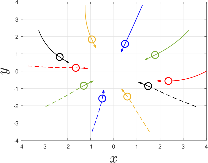
(b) Time 100

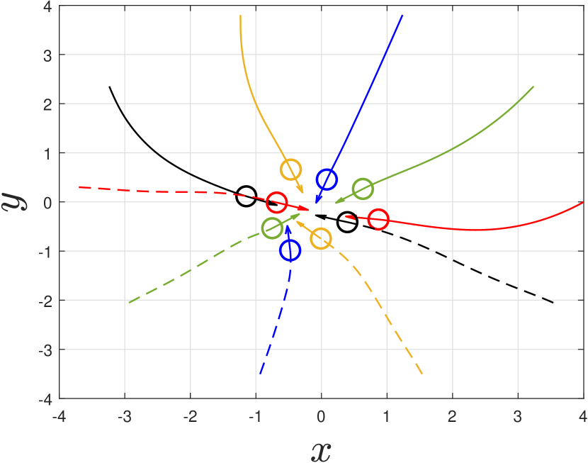
(c) Time 200

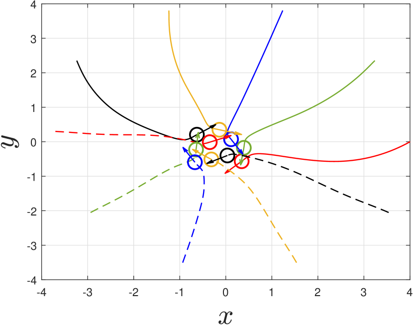
(d) Time 300

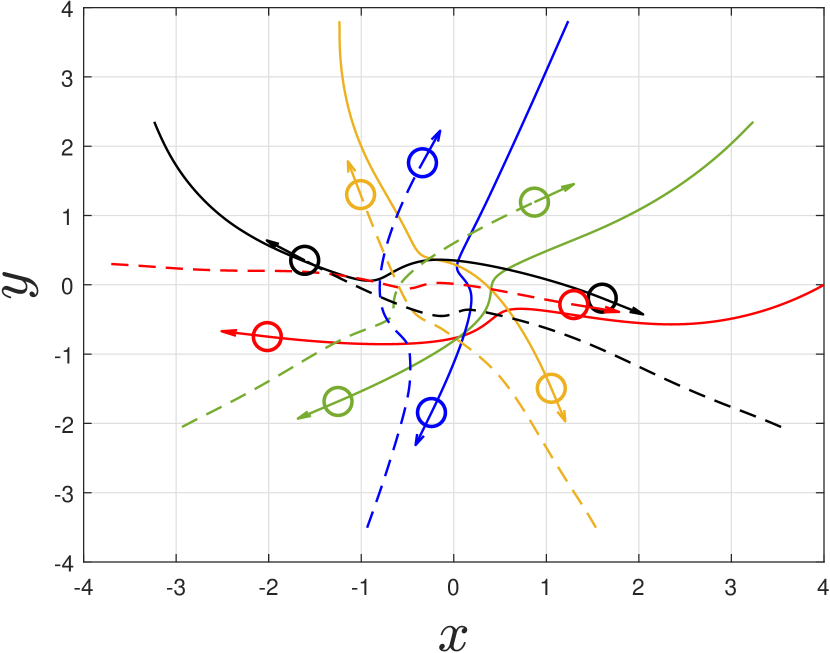
(e) Time 400

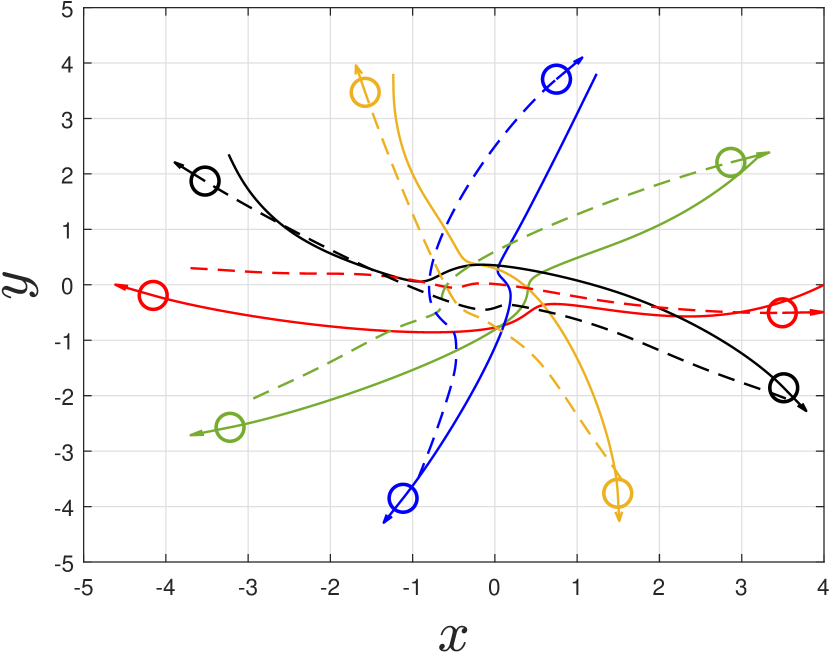
(f) Time 500

Figure 1: Trajectory of ten robots swapping positions according to Algorithm 1. Robots with the same color are swapping positions, and avoiding collision with the others.

5.3 Distributed Control: Truncated Algorithm

The truncated Algorithm 2 is then implemented for the same setting, the truncation parameter $\eta=30$.

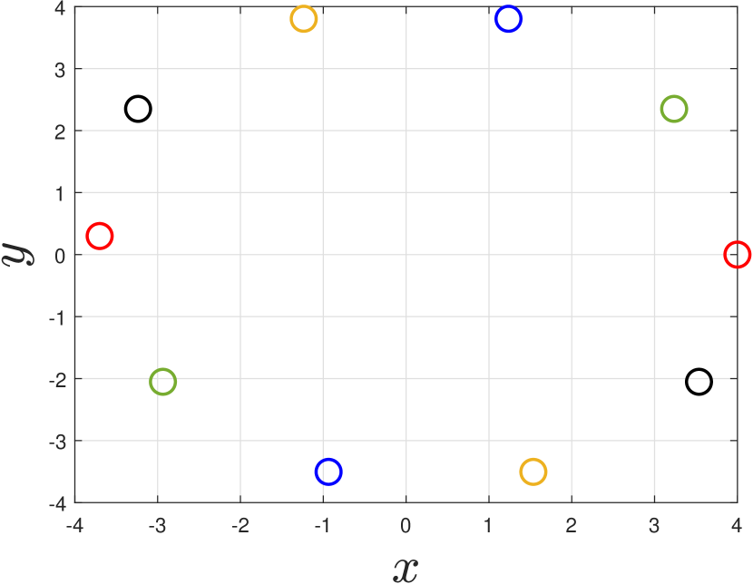
(a) Time 1

(b) Time 100

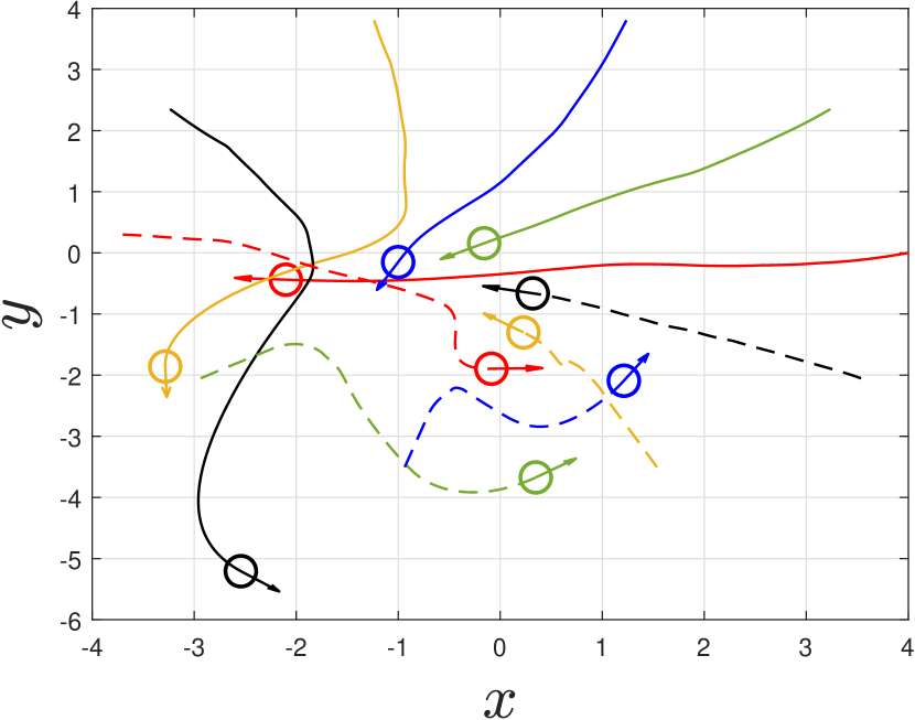
(c) Time 200

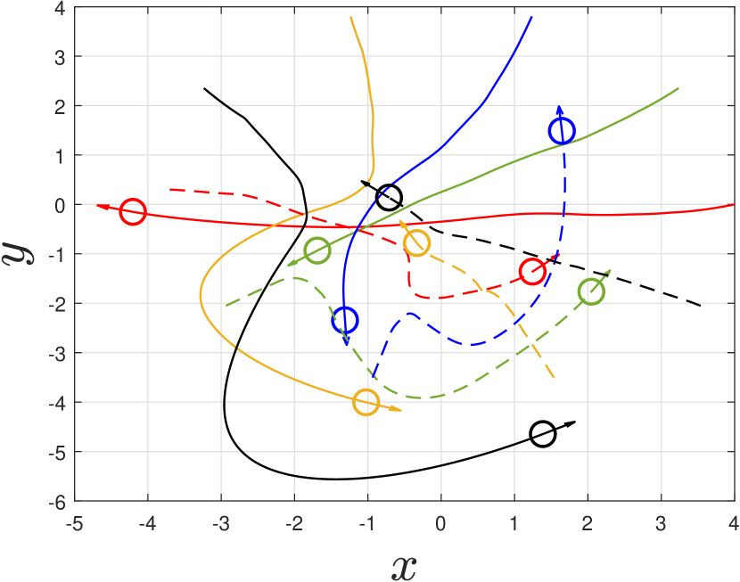
(d) Time 300

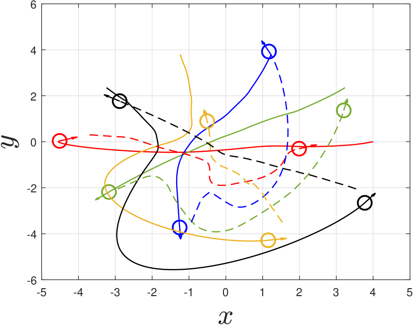
(e) Time 400

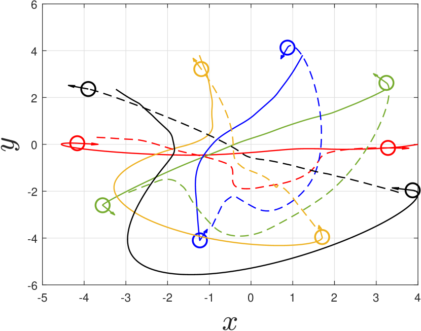
(f) Time 500

Figure 2: Trajectory of ten robots swapping positions while avoiding collision by means of Algorithm 2, with $\eta=30$.

The resulting swapping trajectories are shown in Figure 2. Define

$$\rho_{\mathrm{sum}}^{k} =\sum_{i=1}^{N}\sum_{e\in\mathcal{C}_{i}}\left((\rho_{ie}^{k})^{2}+M_{i}\rho_{ie}^{k}\right).$$ (27)

The evolution of the relaxation parameters $\rho_{\mathrm{sum}}^{0}(\bm{x})$ and $\rho_{\mathrm{sum}}^{30}(\bm{x})$ at each time step along the trajectory is shown in Figures 3(a) and 3(b). It can be seen that $\rho_{\mathrm{sum}}^{30}$ is close to zero at every time step, even $\rho_{\mathrm{sum}}^{0}$ is relatively large at some time steps. This empirically demonstrates the safety guarantees performance of the proposed distributed algorithm. From our experience, $\eta$ could be much smaller for a practical implementation.

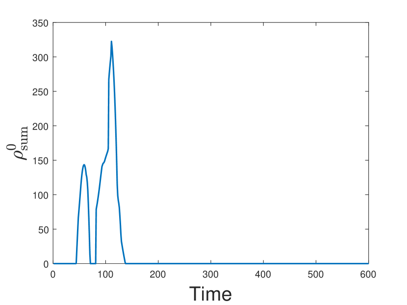
(a) $\rho_{\mathrm{sum}}^{0}(\bm{x})$ along the trajectory

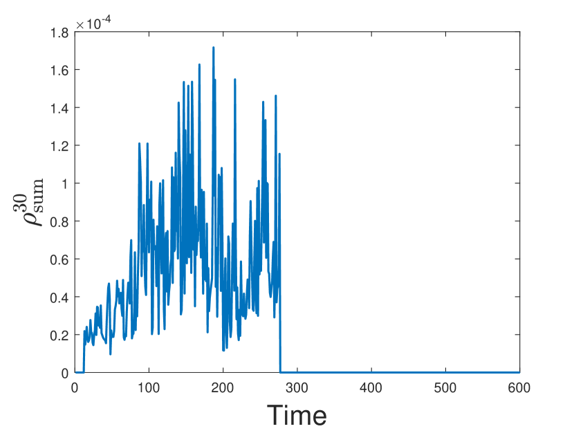
(b) $\rho_{\mathrm{sum}}^{30}(\bm{x})$

along the trajectory

Figure 3: Evolution of the relaxation parameters $\rho_{\mathrm{sum}}^{0}(\bm{x})$ and $\rho_{\mathrm{sum}}^{30}(\bm{x})$ evaluated at the state trajectory, across algorithm iterations.

5.4 Distributed Safety Verification

Safety verification is performed for a four-robot system, within the working space $\mathcal{X}$, defined as $\{p:||p||\leq p^{\mathrm{\max}}=6\}\times\{v:||v||\leq v^{\mathrm{\max}}=1\}$. Each robot is using Algorithm 2 to safely move towards the origin. We sample $200$ scenarios via Algorithm 3. Theorem 13 yields then that with confidence at least $0.9$, $\mathbb{P}\left\{\bm{x}\in{\mathcal{H}}:0\notin\mathcal{Z}\right\}\in[0,0.146]$. We repeat this procedure $300$ times, each time using $300$ scenarios, and construct the empirical cumulative distribution function of $\mathbb{P}\left\{\bm{x}\in{\mathcal{H}}:0\notin\mathcal{Z}\right\}$. This is shown in Figure 4; it can be observed that the empirical probability that $\mathbb{P}\left\{\bm{x}\in{\mathcal{H}}:0\notin\mathcal{Z}\right\}\in[0,0.146]\approx 1$, thus satisfying the theoretical confidence lower bound of $0.9$.

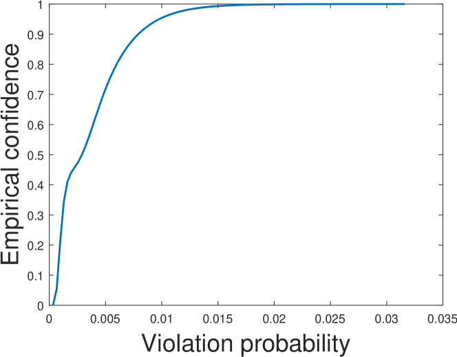
Figure 4: Cumulative distribution function for safety violation.

6 Conclusion

In this paper we presented distributed safe control design and safety verification algorithms for multi-agent systems. The proposed control algorithms introduce auxiliary and relaxation variables to allow feasibility across iterations. We guaranteed convergence to an optimal solution and establish a sublinear convergence rate. We also addressed the problem of distributed safety verification for given control inputs. A scenario-based verification program is formulated and can be solved locally by each agent. The scenarios are sampled independently by a sequential algorithm from the controlled invariant set. The distributed scenario program characterizes the probability of being unsafe, with both lower and upper bounds being determined. Simulation on a multi-robot swapping position problem determines the efficacy of our result. Current work concentrates in accounting for communication delays and model uncertainty in real systems.

Appendix A Appendix

[Proof of Lemma 9] The dual function of (3) is given by

$$q(\bm{\mu}) =\inf_{\{u_{i}\in\mathcal{U}_{i}\},\bm{\rho}\geq 0}\sum_{i=1}^{N}\left\{J_{i}(u_{i})+\sum_{e\in\mathcal{C}_{i}}(\rho^{2}_{ie}+M_{i}\rho_{ie})\right\}$$

$$+\sum_{e=1}^{E}\mu_{e}\left\{\sum_{i\in\mathcal{V}_{e}}h_{ie}(u_{i})-\sum_{i\in\mathcal{V}_{e}}\rho_{ie}\right\}$$

$$=\inf_{\{u_{i}\in\mathcal{U}_{i}\},\bm{\rho}\geq 0}\sum_{i=1}^{N}\left\{J_{i}(u_{i})+\sum_{e\in\mathcal{C}_{i}}\mu_{e}h_{ie}(u_{i})\right\}$$

$$+\sum_{e=1}^{E}\sum_{i\in\mathcal{V}_{e}}\left\{\rho_{ie}^{2}+(M_{i}-\mu_{e})\rho_{ie}\right\}$$ (28)

If there exists $e=1,\ldots,E$, and $i\in\mathcal{V}_{e}$, such that $M_{i}-\mu_{e}<0$, then the minimizer of $\sum_{e=1}^{E}\sum_{k\in\mathcal{V}_{e}}\{\rho_{ie}^{2}+(M_{i}-\mu_{e})\rho_{ie}\}$ is given by $\bm{\rho}^{*}>0$. Notice that this is an unconstrained QP, so its minimizer can be determined by setting its gradient with respect to $\rho_{ie}$ to zero. On the other hand if $M_{i}-\mu_{e}\geq 0$, for all $e=1,\ldots,E,i\in\mathcal{V}_{e}$, the unconstrained minimizer for $\bm{\rho}$ is negative, hence the constrained minimizer $\bm{\rho}^{*}=0$ as $\bm{\rho}\geq 0$. For this case, we obtain

$$\begin{split}q(\bm{\mu})&=\inf_{\{u_{i}\in\mathcal{U}_{i}\}}\sum_{i=1}^{N}\left\{J_{i}(u_{i})+\sum_{e\in\mathcal{C}_{i}}\mu_{e}h_{ie}(u_{i})\right\},\\ \end{split}$$ (29)

which is the dual function for the original unrelaxed problem (3). Recall that (3) is a strictly convex quadratic problem, then $\bm{u}_{\mathrm{rel}}^{*}(\bm{x})=\bm{u}_{\mathrm{nom}}^{*}(\bm{x})$ if $M_{i}\geq\mu_{e}$, for all $e=1,\ldots,E$, $i\in\mathcal{V}_{e}$ since $\bm{\rho}^{*}=0$. The cost function $H(\bm{u},\bm{\rho})$ is strongly convex with Lipschitz continuous gradient since every $J_{i}(u_{i})$ is a strongly convex quadratic function with respect to $u_{i}$, and $\sum_{e\in\mathcal{C}_{i}}(\rho_{ie}^{2}+M_{i}\rho_{ie})$ is strongly convex with respect to $\rho_{ie}$.

[Proof of Theorem 11] We begin with (a). The proof follows a similar idea as [40, Theorem II.6], we only scratch the primal-dual exploration here. Under Assumption 8, strongly duality holds for the primal problem (3) and the dual problem (A). To solve the dual problem $\max_{\bm{\mu}\geq 0}q(\bm{\mu})$ in a distributed manner, an equivalent decomposed problem [40, Section 3.1.3] is formulated as

$$\begin{split}\max_{\bm{\mu}_{i}\geq 0}~{}&\sum_{i=1}^{N}q_{i}(\bm{\mu_{i}})\\ \mathrm{subject~{}to}~{}&\bm{\mu}_{i}=\bm{\mu}_{j},(i,j)\in\mathcal{E},\end{split}$$ (30)

where $\bm{\mu}_{i}$ is a local copy of $\bm{\mu}$ for agent $i$. The dual problem of (30) is given by

$$\begin{split}d^{*}=\min_{\bm{\lambda}}d(\bm{\lambda}):=\sum_{i=1}^{N}\sup_{\bm{\mu}_{i}\geq 0}\left(q_{i}(\bm{\mu}_{i})+\bm{\mu}_{i}^{\top}\sum_{j\in\mathcal{N}_{i}}(\lambda_{ij}-\lambda_{ji})\right),\end{split}$$ (31)

where $\lambda_{ij}$ is a free dual variable for the constraint $\bm{\mu}_{i}=\bm{\mu}_{j}$. Strong duality holds between problem (30) and (31) since (30) is an equality constrained concave problem. Using the gradient descent method to solve (31) at each iteration $k$, each agent $i$ performs two steps:

• (i) calculates the gradient $\nabla d(\bm{\lambda}^{k})$: receive $\lambda_{ji}^{k}$, $j\in\mathcal{N}_{i}$, and compute $\bm{\mu}_{i}^{k+1}$ by solving

  $$\max_{\bm{\mu}_{i}\geq 0}\left(q_{i}(\bm{\mu}_{i})+\bm{\mu}_{i}^{\top}\sum_{j\in\mathcal{N}_{i}}(\lambda_{ij}^{k}-\lambda_{ji}^{k})\right)$$ (32)

• (ii) uses gradient descent: receive $\bm{\mu}_{j}^{k+1},$ and update $\lambda_{ij}$ by:

  $$\lambda_{ij}^{k+1}=\lambda_{ij}^{k}-\gamma^{k}(\bm{\mu}_{i}^{k+1}-\bm{\mu}_{j}^{k+1}).$$ (33)

Diminishing step-size is used here as [23]. Specifically, (32) is the dual problem of (11). Strong duality holds for large enough $\bm{\rho}$ as the relaxed CBF constraints hold strictly. Updating (33) is the same as (12) for every agent in iterations. Given that $d(\bm{\lambda})$ is convex, gradient descent guarantees that $d(\bm{\lambda}^{k})$ convergence to the optimal value $d^{*}=J^{*}$ since strong duality holds between (3) and (30), as well as (30) and (31). Moreover, the relaxed problem (3) is strongly (hence also strictly) convex, which indicates uniqueness of the optimal solution $(\bm{u}_{\mathrm{rel}}^{*},\bm{\rho}^{*})$ . Using Lemma 9, we obtain $\bm{u}_{\mathrm{rel}}^{*}=\bm{u}_{\mathrm{nom}}^{*}$, which is the optimal solution of (3).

We then prove $(b)$. We show that $d(\bm{\lambda})$ is a convex quadratic function. First we prove that for every $i=1,\ldots,N$, $q_{i}(\bm{\mu}_{i})$ in (30) is a concave quadratic function. When every $\mathcal{U}_{i}=\mathbb{R}^{m_{i}}$, the relaxed CBF-QP (3) is a linearly constrained quadratic problem. Following the example [41, Section 5.2.4, Eq. 5.28], every $q_{i}(\bm{\mu}_{i})$ is a concave quadratic function. Therefore, problem (30) is a linearly constrained concave quadratic problem. Following [42, Example 3.6] $d(\bm{\lambda})$ is a convex quadratic function, which is necessarily smooth. Using constant step size

$$0<\gamma<\frac{1}{2L},$$ (34)

where $L$ is Lipschitz constant of $\nabla d(\bm{\lambda}),$ in a gradient descent method to minimize a smooth and convex function $d(\bm{\lambda})$, the generated iterates converge sublinearly as

$$d(\bm{\lambda}^{k})-J^{*} \leq\frac{2(d(\bm{\lambda}^{0})-J^{*})||\bm{\lambda^{0}}-\bm{\lambda^{*}}||_{2}^{2}}{2||\bm{\lambda}^{0}-\bm{\lambda}^{*}||_{2}^{2}+k\gamma(2-L\gamma)(d(\bm{\lambda}^{0})-J^{*})}$$

$$\leq \frac{2(d(\bm{\lambda}^{0})-J^{*})||\bm{\lambda^{0}}-\bm{\lambda^{*}}||_{2}^{2}}{k\gamma(d(\bm{\lambda}^{0})-J^{*})}\leq\frac{2||\bm{\lambda}^{0}-\bm{\lambda}^{*}||_{2}^{2}}{k\gamma}.$$ (35)

The first inequality is proved by [43, theorem 2.1.4], the second one comes from eliminating the term $||\bm{\lambda}^{0}-\bm{\lambda}^{*}||_{2}^{2}$, and considering $2-L\gamma\geq 1$ from (34). The Lipschitz constant can be calculated by the largest eigenvalue of the quadratic term for $d(\bm{\lambda})$. Although the expression of $d(\bm{\lambda}^{k})$ is not derived, $d(\bm{\lambda}^{k})$ can be calculated by

$$d(\bm{\lambda}^{k})=\sum_{i=1}^{N}\sup_{\bm{\mu}_{i}\geq 0}\left(q_{i}(\bm{\mu}_{i})+\bm{\mu}_{i}^{\top}\sum_{j\in\mathcal{N}_{i}}(\lambda_{ij}-\lambda_{ji})\right)$$

$$=\sum_{i=1}^{N}\sup_{\bm{\mu}_{i}\geq 0}\left(\inf_{u_{i},\bm{\rho}_{i}\geq 0}\left(J_{i}(u_{i})+\sum_{e\in\mathcal{C}_{i}}\left(\rho_{ie}^{2}+M_{i}\rho_{ie}\right)\right)\right.$$

$$\left.+\sum_{e\in\mathcal{C}_{i}}\mu_{ie}(h_{ie}(u_{i})-\rho_{ie})+\bm{\mu}_{i}^{\top}\sum_{j\in\mathcal{N}_{i}}(\lambda_{ij}^{k}-\lambda_{ji}^{k})\right).$$ (36)

For every $i=1,\ldots,N$, and $\bm{\lambda}^{k}$, there always exists $\bm{u}_{i}$ and $\bm{\rho}_{i}$, such that the inequality constraint in (4) strictly holds, which indicates strong duality. Therefore, we have

$$d(\bm{\lambda}^{k})=$$

$$\sum_{i=1}^{N}\inf_{u_{i},\bm{\rho}_{i}\geq 0}\left(\sup_{\bm{\mu}_{i}\geq 0}\left(J_{i}(u_{i})+\sum_{e\in\mathcal{C}_{i}}\left(\rho_{ie}^{2}+M_{i}\rho_{ie}\right)\right)\right.$$

$$\left.+\sum_{e\in\mathcal{C}_{i}}\mu_{ie}(h_{ie}(u_{i})-\rho_{ie})+\bm{\mu}_{i}^{\top}\sum_{j\in\mathcal{N}_{i}}(\lambda_{ij}^{k}-\lambda_{ji}^{k})\right)$$

$$=\sum_{i=1}^{N}\left(J_{i}(u_{i}^{k}+\sum_{e\in\mathcal{C}_{i}}((\rho_{ie}^{k})^{2}+M_{i}\rho_{ie}^{k})\right)$$

$$=\sum_{i=1}^{N}||u_{i}^{k}-u^{\mathrm{des}}||^{2}+\rho_{\mathrm{sum}}^{k}=H(\bm{u}^{k},\bm{\rho}^{k}).$$ (37)

Hence, by (A) and (A) we conclude that $H(\bm{u}^{k},\bm{\rho}^{k})-J^{*}<\frac{2||\bm{\lambda}^{0}-\bm{\lambda}^{*}||_{2}^{2}}{\gamma k}$.

[Proof of Theorem 13] We have that

$$\mathbb{P}^{\bar{N}} \left\{\frac{\sum_{i=1}^{N}\underline{\epsilon}_{i}(s_{i}^{*})}{N}\leq\mathbb{P}\left\{\bm{x}\in{\mathcal{H}}:\bm{z}^{*}\notin\mathcal{Z}\right\}\leq\sum_{i=1}^{N}\bar{\epsilon}_{i}(s_{i}^{*})\right\}$$

$$=\mathbb{P}^{\bar{N}}\left\{\frac{1}{N}\sum_{i=1}^{N}\underline{\epsilon}_{i}(s_{i}^{*})\leq\mathbb{P}\left\{\vphantom{\bigcap_{i=1}^{N}}\bm{x}\in{\mathcal{H}}:\right.\right.$$

$$\hskip 2.84544pt\exists i\in\{1,\ldots,N\},\left.\left.\vphantom{\bigcap_{i=1}^{N}}\bm{z}^{*}\notin\mathcal{Z}_{i}\right\}\leq\sum_{i=1}^{N}\bar{\epsilon}_{i}(s_{i}^{*})\right\}$$

$$=\mathbb{P}^{\bar{N}}\left\{\frac{1}{N}\sum_{i=1}^{N}\underline{\epsilon}_{i}(s_{i}^{*})\leq\mathbb{P}\left\{\bm{x}\in{\mathcal{H}}:\bigcup_{i=1}^{N}\left\{\bm{z}^{*}\notin\mathcal{Z}_{i}\right\}\right\}\right.$$

$$\bigcap\left.\mathbb{P}\left\{\bigcup_{i=1}^{N}\left\{\bm{x}\in{\mathcal{H}}:\bm{z}^{*}\notin\mathcal{Z}_{i}\right\}\right\}\leq\sum_{i=1}^{N}\bar{\epsilon}_{i}(s_{i}^{*})\right.\}$$ (38)

We separately deal with the inner and upper bounds on the probability. For the upper bound we have

$$\mathbb{P}^{\bar{N}} \left\{\mathbb{P}\left\{\bigcup_{i=1}^{N}\left\{\bm{x}\in{\mathcal{H}}:\bm{z}^{*}\notin\mathcal{Z}_{i}\right\}\right\}\leq\sum_{i=1}^{N}\bar{\epsilon}_{i}(s_{i}^{*})\right\}$$

$$\geq \mathbb{P}^{\bar{N}}\left\{\sum_{i=1}^{N}\mathbb{P}\left\{\bm{x}\in{\mathcal{H}}:\vphantom{\bigcup}\bm{z}^{*}\notin\mathcal{Z}_{i}\right\}\leq\sum_{i=1}^{N}\bar{\epsilon}_{i}(s_{i}^{*})\right\}.$$

The equality is achieved when for any $i\neq j$, $\bm{z}^{*}\notin\mathcal{Z}_{i}$ and $\bm{z}^{*}\notin\mathcal{Z}_{j}$ are mutually exclusive. For the lower bound we have

$$\mathbb{P}^{\bar{N}} \left\{\frac{1}{N}\sum_{i=1}^{N}\underline{\epsilon}_{i}(s_{i}^{*})\leq\mathbb{P}\left\{\bm{x}\in{\mathcal{H}}:\bigcup_{i=1}^{N}\left\{\bm{z}^{*}\notin\mathcal{Z}_{i}\right\}\right\}\right\}$$

$$\geq \mathbb{P}^{\bar{N}}\left\{N\cdot\frac{1}{N}\sum_{i=1}^{N}\underline{\epsilon}_{i}(s_{i}^{*})\leq\sum_{i=1}^{N}\mathbb{P}\left\{\bm{x}\in{\mathcal{H}}:\vphantom{\bigcup}\bm{z}^{*}\notin\mathcal{Z}_{i}\right\}\right\}.$$

The equality is achieved if for any $i\neq j$, $\bm{z}^{*}\neq\mathcal{Z}_{i}\Leftrightarrow\bm{z}\neq\mathcal{Z}_{j}$ and $\underline{\epsilon}_{i}(s_{i}^{*})=\underline{\epsilon}_{j}(s_{j}^{*})$. The right-hand side of (A) can be then lower-bounded by

$$\mathbb{P}^{\bar{N}}\left\{N\cdot\frac{1}{N}\sum_{i=1}^{N}\underline{\epsilon}_{i}(s_{i}^{*})\leq\sum_{i=1}^{N}\mathbb{P}\left\{\bm{x}\in{\mathcal{H}}:\vphantom{\bigcup}\bm{z}^{*}\notin\mathcal{Z}_{i}\right\}\right.$$

$$\bigcap\left.\sum_{i=1}^{N}\mathbb{P}\left\{\bm{x}\in{\mathcal{H}}:\vphantom{\bigcup}\bm{z}^{*}\notin\mathcal{Z}_{i}\right\}\leq\sum_{i=1}^{N}\bar{\epsilon}_{i}(s_{i}^{*})\right\}$$

$$\geq\mathbb{P}^{\bar{N}}\left\{\bigcap_{i=1}^{N}\left\{\underline{\epsilon}_{i}(s_{i}^{*})\leq\mathbb{P}\left\{\bm{x}\in{\mathcal{H}}:\vphantom{\bigcup}\bm{z}^{*}\notin\mathcal{Z}_{i}\right\}\leq\bar{\epsilon}_{i}(s_{i}^{*})\right\}\right\}$$

$$\geq 1-\sum_{i=1}^{N}\mathbb{P}^{\bar{N}}\left\{\bar{\epsilon}_{i}(s_{i}^{*})<\mathbb{P}\left\{\bm{x}\in{\mathcal{H}}:\vphantom{\bigcup}\bm{z}^{*}\notin\mathcal{Z}_{i}\right\}\right.$$

$$\bigcup\left.\mathbb{P}\left\{\bm{x}\in{\mathcal{H}}:\vphantom{\bigcup}\bm{z}^{*}\notin\mathcal{Z}_{i}\right\}<\underline{\epsilon}_{i}(s_{i}^{*})\right\}.$$ (39)

By [30, Theorem 1] we have that for any $i=1,\ldots,N$

$$\mathbb{P}^{\bar{N}}\left\{\bm{x}\in{\mathcal{H}}:\underline{\epsilon}_{i}(s_{i}^{*})\leq\mathbb{P}\left\{\vphantom{\bigcup}\bm{x}\in{\mathcal{H}}:\bm{z}^{*}\notin\mathcal{Z}_{i}\right\}\leq\bar{\epsilon}_{i}(s_{i}^{*})\right\}$$

$$\geq 1-\beta_{i}$$

$$\Rightarrow \sum_{i=1}^{N}\mathbb{P}^{\bar{N}}\left\{\bar{\epsilon}_{i}(s_{i}^{*})<\mathbb{P}\left\{\bm{x}\in{\mathcal{H}}:\vphantom{\bigcup}\bm{z}^{*}\notin\mathcal{Z}_{i}\right\}\right.$$

$$\bigcup\left.\mathbb{P}\left\{\bm{x}\in{\mathcal{H}}:\vphantom{\bigcup}\bm{z}^{*}\notin\mathcal{Z}_{i}\right\}<\underline{\epsilon}_{i}(s_{i}^{*})\right\}<\sum_{i=1}^{N}\beta_{i}.$$ (40)

Since $\frac{\underline{\epsilon}(s^{*})}{N}<\underline{\epsilon}(s^{*})<\bar{\epsilon}(s^{*})$, substituting (A) into (A) with $i=1,\ldots,N$ we obtain

$$\mathbb{P}^{\bar{N}}\left\{\frac{\underline{\epsilon}(s^{*})}{N}\leq\mathbb{P}\left\{\bm{x}\in{\mathcal{H}}:\bm{z}^{*}\notin\mathcal{Z}\right\}\leq\bar{\epsilon}(s^{*})\right\}\geq 1-\beta.$$ (41)

We then prove that $\bm{z}^{*}$ is unique, and $\bm{z}^{*}=0$. For the case where all the CBF constraints are satisfied, i.e. $\sum_{k\in\mathcal{V}_{e}}h_{ke}(u_{k}(\bm{x}^{(r)}))\leq 0,\forall e=1,\ldots,E$, $r=1,\ldots,\bar{N}$, we have that $\bm{z}^{*}=0$ and $\bm{\zeta}^{*}=0$. For the case where there exists violated CBF constraint, i.e. $\sum_{i\in\mathcal{V}_{e}}h_{ie}(u_{i}(\bm{x}^{(r)}))>0$, we have that $z_{ie}^{*}=0$ since $\bm{z}\leq 0$, and $\zeta_{ie}^{*}>0$ for $i\in\mathcal{V}_{e}$. In summary, we always have $\bm{z}^{*}=0$ for any scenarios, thus (41) is equivalent to (22). In addition, we directly obtain that $\zeta_{ie}^{*}>0$ shows that $\sum_{i\in\mathcal{V}_{e}}h_{ie}(u_{i}(\bm{x}^{(r)}))>z_{ie}^{*}=0$. Thus, for every agent, $s_{i}^{*}$ is the number of non-zero $\zeta_{ie}^{*}$, for $e\in\mathcal{C}_{i}$.

References

• [1] H. Wang, A. Papachristodoulou, and K. Margellos, “Distributed safety verification for multi-agent systems,” 62nd IEEE Conference on Decision and Control, 2023.
• [2] F. Ding, J. He, Y. Ren, H. Wang, and Y. Zheng, “Configuration-aware safe control for mobile robotic arm with control barrier functions,” arXiv preprint arXiv:2204.08265, 2022.
• [3] H. Wang, Y. Li, W. Yu, J. He, and X. Guan, “Moving obstacle avoidance and topology recovery for multi-agent systems,” in American Control Conference (ACC), pp. 2696–2701, IEEE, 2019.
• [4] J. Axelsson, “Safety in vehicle platooning: A systematic literature review,” IEEE Transactions on Intelligent Transportation Systems, vol. 18, no. 5, pp. 1033–1045, 2016.
• [5] A. Alam, A. Gattami, K. H. Johansson, and C. J. Tomlin, “Guaranteeing safety for heavy duty vehicle platooning: Safe set computations and experimental evaluations,” Control Engineering Practice, vol. 24, pp. 33–41, 2014.
• [6] W. Xiao and C. G. Cassandras, “Decentralized optimal merging control for connected and automated vehicles with safety constraint guarantees,” Automatica, vol. 123, p. 109333, 2021.
• [7] A. D. Ames, X. Xu, J. W. Grizzle, and P. Tabuada, “Control barrier function based quadratic programs for safety critical systems,” IEEE Transactions on Automatic Control, vol. 62, no. 8, pp. 3861–3876, 2016.
• [8] E. D. Sontag, “A ‘universal’construction of artstein’s theorem on nonlinear stabilization,” Systems & control letters, vol. 13, no. 2, pp. 117–123, 1989.
• [9] J. A. Primbs, V. Nevistić, and J. C. Doyle, “Nonlinear optimal control: A control lyapunov function and receding horizon perspective,” Asian Journal of Control, vol. 1, no. 1, pp. 14–24, 1999.
• [10] S.-C. Hsu, X. Xu, and A. D. Ames, “Control barrier function based quadratic programs with application to bipedal robotic walking,” in 2015 American Control Conference (ACC), pp. 4542–4548, IEEE, 2015.
• [11] A. D. Ames, J. W. Grizzle, and P. Tabuada, “Control barrier function based quadratic programs with application to adaptive cruise control,” in 53rd IEEE Conference on Decision and Control, pp. 6271–6278, IEEE, 2014.
• [12] Y. Chen, A. Singletary, and A. D. Ames, “Guaranteed obstacle avoidance for multi-robot operations with limited actuation: A control barrier function approach,” IEEE Control Systems Letters, vol. 5, no. 1, pp. 127–132, 2020.
• [13] L. Wang, A. D. Ames, and M. Egerstedt, “Safety barrier certificates for collisions-free multirobot systems,” IEEE Transactions on Robotics, vol. 33, no. 3, pp. 661–674, 2017.
• [14] U. Borrmann, L. Wang, A. D. Ames, and M. Egerstedt, “Control barrier certificates for safe swarm behavior,” IFAC-PapersOnLine, vol. 48, no. 27, pp. 68–73, 2015.
• [15] X. Xu, “Constrained control of input–output linearizable systems using control sharing barrier functions,” Automatica, vol. 87, pp. 195–201, 2018.
• [16] X. Tan and D. V. Dimarogonas, “Distributed implementation of control barrier functions for multi-agent systems,” IEEE Control Systems Letters, vol. 6, pp. 1879–1884, 2021.
• [17] A. Falsone, K. Margellos, S. Garatti, and M. Prandini, “Dual decomposition for multi-agent distributed optimization with coupling constraints,” Automatica, vol. 84, pp. 149–158, 2017.
• [18] A. Falsone, I. Notarnicola, G. Notarstefano, and M. Prandini, “Tracking-admm for distributed constraint-coupled optimization,” Automatica, vol. 117, p. 108962, 2020.
• [19] W. Shi, Q. Ling, K. Yuan, G. Wu, and W. Yin, “On the linear convergence of the admm in decentralized consensus optimization,” IEEE Transactions on Signal Processing, vol. 62, no. 7, pp. 1750–1761, 2014.
• [20] J. C. Duchi, A. Agarwal, and M. J. Wainwright, “Dual averaging for distributed optimization: Convergence analysis and network scaling,” IEEE Transactions on Automatic control, vol. 57, no. 3, pp. 592–606, 2011.
• [21] K. Margellos, A. Falsone, S. Garatti, and M. Prandini, “Distributed constrained optimization and consensus in uncertain networks via proximal minimization,” IEEE Transactions on Automatic Control, vol. 63, no. 5, pp. 1372–1387, 2017.
• [22] A. Camisa, F. Farina, I. Notarnicola, and G. Notarstefano, “Distributed constraint-coupled optimization via primal decomposition over random time-varying graphs,” Automatica, vol. 131, p. 109739, 2021.
• [23] I. Notarnicola and G. Notarstefano, “Constraint-coupled distributed optimization: A relaxation and duality approach,” IEEE Transactions on Control of Network Systems, vol. 7, no. 1, pp. 483–492, 2019.
• [24] X. Li, G. Feng, and L. Xie, “Distributed proximal algorithms for multiagent optimization with coupled inequality constraints,” IEEE Transactions on Automatic Control, vol. 66, no. 3, pp. 1223–1230, 2020.
• [25] A. Nedic, A. Ozdaglar, and P. A. Parrilo, “Constrained consensus and optimization in multi-agent networks,” IEEE Transactions on Automatic Control, vol. 55, no. 4, pp. 922–938, 2010.
• [26] M. C. Campi and S. Garatti, “The exact feasibility of randomized solutions of uncertain convex programs,” SIAM Journal on Optimization, vol. 19, no. 3, pp. 1211–1230, 2008.
• [27] M. C. Campi and S. Garatti, “Wait-and-judge scenario optimization,” Mathematical Programming, vol. 167, no. 1, pp. 155–189, 2018.
• [28] G. Calafiore and M. C. Campi, “Uncertain convex programs: randomized solutions and confidence levels,” Mathematical Programming, vol. 102, no. 1, pp. 25–46, 2005.
• [29] G. C. Calafiore and M. C. Campi, “The scenario approach to robust control design,” IEEE Transactions on Automatic Control, vol. 51, no. 5, pp. 742–753, 2006.
• [30] S. Garatti and M. C. Campi, “Risk and complexity in scenario optimization,” Mathematical Programming, pp. 1–37, 2019.
• [31] K. Margellos and J. Lygeros, “Hamilton–Jacobi formulation for reach–avoid differential games,” IEEE Transactions on Automatic Control, vol. 56, no. 8, pp. 1849–1861, 2011.
• [32] J. Lygeros, “On reachability and minimum cost optimal control,” Automatica, vol. 40, no. 6, pp. 917–927, 2004.
• [33] S. Prajna and A. Jadbabaie, “Safety verification of hybrid systems using barrier certificates,” in International Workshop on Hybrid Systems: Computation and Control, pp. 477–492, Springer, 2004.
• [34] S. Prajna, A. Jadbabaie, and G. J. Pappas, “A framework for worst-case and stochastic safety verification using barrier certificates,” IEEE Transactions on Automatic Control, vol. 52, no. 8, pp. 1415–1428, 2007.
• [35] S. Prajna, A. Papachristodoulou, and P. A. Parrilo, “Introducing sostools: A general purpose sum of squares programming solver,” in Proceedings of the 41st IEEE Conference on Decision and Control, 2002., vol. 1, pp. 741–746, IEEE, 2002.
• [36] S. Prajna, A. Papachristodoulou, P. Seiler, and P. A. Parrilo, “Sostools: Sum of squares optimization toolbox for matlab,” 2004.
• [37] P. Akella and A. D. Ames, “A barrier-based scenario approach to verifying safety-critical systems,” IEEE Robotics and Automation Letters, 2022.
• [38] A. Taly and A. Tiwari, “Deductive verification of continuous dynamical systems,” in IARCS Annual Conference on Foundations of Software Technology and Theoretical Computer Science, Schloss Dagstuhl-Leibniz-Zentrum für Informatik, 2009.
• [39] D. G. Wright, “Tychonoff’s theorem,” Proceedings of the American Mathematical Society, vol. 120, no. 3, pp. 985–987, 1994.
• [40] G. Notarstefano, I. Notarnicola, A. Camisa, et al., “Distributed optimization for smart cyber-physical networks,” Foundations and Trends® in Systems and Control, vol. 7, no. 3, pp. 253–383, 2019.
• [41] S. Boyd, S. P. Boyd, and L. Vandenberghe, Convex optimization. Cambridge university press, 2004.
• [42] V. Guigues, “On the strong concavity of the dual function of an optimization problem,” arXiv preprint arXiv:2006.16781, 2020.
• [43] Y. Nesterov, Introductory lectures on convex optimization: A basic course, vol. 87. Springer Science & Business Media, 2003.