Scalable Bayesian bi-level variable selection in generalized linear models

Abstract

Motivated by a real-world application in cardiology, we develop an algorithm to perform Bayesian bi-level variable selection in a generalized linear model, for datasets that may be large both in terms of the number of individuals and the number of predictors. Our algorithm relies on the waste-free SMC (Sequential Monte Carlo) methodology of Dau and Chopin, (2022), a new proposal mechanism to deal with the constraints specific to bi-level selection (which forbid to select an individual predictor if its group is not selected), and the ALA (approximate Laplace approximation) approach of Rossell et al., (2021). We show in our numerical study that the algorithm may offer reliable performance on large datasets within a few minutes, on both simulated data and real data related to the aforementioned cardiology application.

Keywords Approximate Laplace approximation  $\cdot$ Bi-level variable selection  $\cdot$ Sequential Monte Carlo  $\cdot$ waste-free Sequential Monte Carlo

1 Introduction

1.1 Motivation

While useful more generally, the approach developed in this paper was initially motivated by a public health dataset recording the medical history of a large number of individuals that may or may not have suffered from sudden cardiac death (SCD); this dataset will be described more fully later. One may use this data to determine whether consumption of medical drugs or hospitalization may increase the odds of an SCD event. Unfortunately, the number of potential drugs and diseases is very large, and their incidence in the studied population vary a lot. This makes it difficult to assess the impact of drugs and diseases that are rarely prescribed or observed. On the other hand, there are official nomenclatures for drugs and diseases, which can be classified into groups with similar properties. Hospital diagnoses are coded according to the International Classification of Diseases and drugs are coded according to the Anatomical Therapeutic Chemical system, that classifies them according to the organ or system on which they act and their therapeutic, pharmacological, and chemical properties. Therefore, there is clear medical interest in determining automatically whether there is enough information in the data to indicate that a particular drug or disease affects SCD, or, if not, whether the group it belongs to does.

This led us to develop a bi-level variable selection procedure, based on a binary regression (outcome variable is whether the individual had an SCD event) model, and which should work reliably for a fairly large number of individuals, variables and groups. In addition, we wanted this procedure to be Bayesian, in order to be able to obtain posterior probabilities of inclusion (rather than simply 0/1 answers).

There are surprising few papers on Bayesian bi-level variable selection, and most of them focus on linear regression with Gaussian noise (Chen et al.,, 2016; Mallick and Yi,, 2017; Cai et al.,, 2020). For such a model, one may integrate out the regression coefficients (the prior provided is Gaussian) to obtain the marginal posterior distribution over a finite space (the inclusion of either individual variables or groups). Even so, designing a MCMC able to efficiently explore that finite space is challenging. Such discrete distributions tend to exhibit strongly separated modal regions, and a MCMC chain may fail to escape one of this region. We refer in particular to the numerical experiments of Schäfer and Chopin, (2013) that show that various MCMC schemes may lead to unstable estimates because of this problem. Of course, this issue gets worse when the number of variables increases, making MCMC unable to scale properly with datasets with a large number of variables (and groups).

1.2 Proposed approach

Schäfer and Chopin, (2013) designed a tempering SMC sampler for standard (one-level) variable selection for linear regressions, and showed it outperformed significantly MCMC, as explained above. We adapt this approach to our problem in three ways. First, we replace it by a waste-free SMC sampler, following Dau and Chopin, (2022), as waste-free SMC tends to outperform standard SMC. Waste-free SMC amounts to resampling only a fraction of the particles, then moving them through numerous MCMC steps, and keeping all these intermediate. Second, we adapt the proposal mechanism within the MCMC step so as to accommodate the constraints specific to bi-level selection (namely, that a variable may be selected only if its group is selected).

Third, we replace the intractable marginal likelihood (obtained by integrating out the regression coefficients) by either its LA (Laplace approximation), or by a cheaper approximation introduced by Rossell et al., (2021), called ALA (approximate LA). The reason why ALA is particularly attractive in our context is that it scales very well with respect to $n$ (as we explain later). We assess in our numerical experiments the impact of the error introduced by ALA on the actual results. We note that Schäfer, (2012) already showed in his PhD thesis that replacing the marginal likelihood by its LA within a SMC sampler (targeting a variable selection posterior) incurs only a negligible bias.

1.3 Plan

Section 2 describes the considered class of model, the bi-level variable selection problem, and the related notations. Section 3 describes the proposed algorithm, starting with a generic (waste-free) SMC sampler, and explaining how this generic algorithm may be adapted to bi-level variable selection. Section 4 assesses (statistically and numerically) the proposed approach through two numerical experiments, one on simulated data and one on the public health dataset mentioned in the introduction.

2 Model

2.1 Regression model

For the sake of concreteness, we consider the following binary regression model, although our approach could easily be generalised to other generalised linear models. We suppose that we have collected a dataset $\mathcal{D}=\left\{X,U,Z,y\right\}$ with sample size $n$, where $y\in\left\{0,1\right\}^{n}$ is a vector of binary responses, $X=(x_{ij})\in\mathbb{R}^{n\times p}$, $U=(u_{ij})\in\mathbb{R}^{n\times q}$, and $Z=(z_{ij})\in\mathbb{R}^{n\times r}$, are design matrices that contain, respectively, ‘individual variables’, ‘group variables’ (both subject to variable selection later on), and extra variables that the user wants to include systematically (e.g. the intercept, socio-demographic effects such as sex, age, etc.).

Regarding the group structure, we assume that each of the $p$ variables in $X$ belongs to one (and only one) of the $q$ groups; let $g(j)$ be the group of variable $j$. A group variable (in $U$) may represent different types of ‘group effects’. For instance, in a medical application, the variables in a group $k$ may be the indicator that the patient took a certain drug in the last six months, and the group variable may be the indicator that a patient took any drug in that group in the same period. Alternatively, these variables could be the number of drug intakes for each drug; in that case, the group variable would be the number of intakes of drugs in that group. In either scenarios, the point is to determine whether one may measure a significant effect for each individual variable, on top of the group effect, or a significant effect for its group only, or neither.

To sum up, without variable selection, the distribution of each data point would be such that, for $i=1,\ldots,n$:

$$P(Y_{i}=1|\beta)=F\left(\sum_{j=1}^{p}\beta_{j}^{x}x_{ij}+\sum_{k=1}^{q}\beta_{k}^{u}u_{ik}+\sum_{l=1}^{r}\beta_{l}^{z}z_{il}\right)$$ (1)

and $P(Y_{i}=0|\beta)=1-P(Y_{i}=1|\beta)$, where $\beta=(\beta^{x},\beta^{u},\beta^{z})$ is the vector of regression parameters, $F$ is the link function (e.g. $F=\Phi$, the unit Gaussian CDF for a probit model). We assign independent Gaussian priors to the regression coefficients: $p(\beta^{z})\sim\mathcal{N}(0_{r},\sigma^{2}\text{I}_{r}),p(\beta^{u})\sim\mathcal{N}(0_{q},\sigma^{2}\text{I}_{q})$ and $p(\beta^{x})\sim\mathcal{N}(0_{p},\sigma^{2}\text{I}_{p})$.

2.2 Bi-level variable selection

We extend our model to perform selection of groups and variables simultaneously. Most of existing models lack flexibility as they impose only “all-in” or “all-out” selection for variables in the same group. That is, if a group is not selected by the model, variables belonging to this group will also not be selected. In this work, we propose a more general approach in order to capture sparsity at both the group and variable levels. To this end, we introduce $\theta=(\gamma,\eta)$, a set of two types of binary variables: $\gamma_{k}$ indicates whether group $k$ is active ($\gamma_{k}=1$) or not ($\gamma_{k}=0$), and $\eta_{j}$ indicates whether individual variable $j$, which is in group $g(j)$, is active ($\eta_{j}=1$) or not ($\eta_{j}=0)$. We consider a hierarchical structure such that the variable $j$ is not selected if $\gamma_{g(j)}=0$, that is $P(\eta_{j}=1|\gamma_{k}=0)=0$ for $k=g(j)$. As compared to existing models, we propose to keep the flexibility of selecting variables within a group. For example, when a group of drugs is related to SCD, it does not necessarily mean that all drugs of this group are related to SCD. Therefore, we may want to not only remove unimportant groups effectively, but also identify important variables within important groups as well. Thus, we replace (1) by

$$P(Y_{i}=1|\beta,\theta)=F\left(\sum_{j=1}^{p}\eta_{j}\beta_{j}^{x}x_{ij}+\sum_{k=1}^{q}\gamma_{k}\beta_{k}^{u}u_{ik}+\sum_{l=1}^{r}\beta_{l}^{z}z_{il}\right).$$ (2)

Let $p(\gamma)$ be the prior density of $\gamma$, which is a product of Bernoulli distributions with probabilities $p_{j}^{\gamma}$. For the predictors, we introduce a spike-and-slab prior defined by

$$P(\eta_{j}=1|\gamma)=\begin{cases}p_{j}^{\eta}&\text{if }\gamma_{g(j)}=1\\ 0&\text{otherwise.}\end{cases}$$ (3)

This bi-level structure implies that variable $j$ may be selected only if the group it belongs to, $g(j)$, is selected.

To perform Bayesian bi-level variable selection, we aim to approximating the (marginal) posterior distribution of $\theta=(\gamma,\eta)$, i.e. $\pi(\theta)=p(\theta|\mathcal{D})\propto p(\theta)L(\theta)$, where $p(\theta)$ is the prior described above, and $L(\theta)$ is the integrated likelihood obtained by integrating out $\beta$:

$$L(\theta)=\int L(\beta,\theta)p(\beta)d\beta,\qquad L(\beta,\theta)=\left\{\prod_{i=1}^{N}P(Y_{i}=y_{i}|\beta,\theta)\right\}.$$

3 The proposed algorithm

3.1 Tempering waste-free SMC

We propose a tempering waste-free Sequential Monte Carlo (SMC) sampler to approximate the joint posterior distribution $\pi(\theta)=p(\theta|\mathcal{D})$. SMC methods are iterative stochastic algorithms that approximate a sequence of probability distributions through successive importance sampling, resampling and Markov steps. In Bayesian modeling, this sequence can be used to interpolate between a distribution $p(\theta)$ which is easy to sample from (e.g. the prior distribution) and a distribution of interest $\pi(\theta)$ which may be difficult to simulate directly (i.e. the posterior distribution). The tempering approach in particular is based on a sequence of tempered distributions of the form

$$\forall t\geq 1,\;\pi_{t}(\theta)=\frac{p(\theta)L(\theta)^{\lambda_{t}}}{Z_{t}}$$

where $p(\theta)$ is the prior density, $L(\theta)$ the likelihood, $Z_{t}>0$ is the normalising constant and $0=\lambda_{0}<\lambda_{1}<\ldots<\lambda_{T}=1$ is a sequence increasing from 0 to 1. This geometric bridge smoothly interpolates between the initial distribution $p(\theta)$ and the target distribution $\pi(\theta)\propto p(\theta)L(\theta)$.

A typical application of such an approach is the simulation of a multimodal distribution $\pi$. Since simulating directly from such a distribution is difficult, we may use tempering SMC instead, to sample initially from a distribution $p$ which covers the support of $\pi$, and to move progressively towards $\pi$ through intermediate distributions that are progressively more and more multimodal. In this work, we combined the tempering approach with the waste-free SMC sampler proposed by Dau and Chopin, (2022). The main idea of this scheme is to resample only $M$ ancestors from the $N$ particles in the standard SMC sampler (with $M\ll N$). Each of the ancestors is then moved $P-1$ times through a Markov kernel $K_{t}$. The $M$ chains of length $P$ are finally put together to form a new particle sample of size $N=MP$. Algorithm 1 describes the corresponding algorithm for a tempering sequence. At the final iteration $T$ of the algorithm, one may approximate any expectation $\mathbb{E}_{\pi}\varphi(\theta)$ with $\sum_{n=1}^{N}W_{T}^{n}\varphi(\theta_{T}^{n})$, where the $W_{T}^{n}$ are the normalised weights at the final iteration $T$.

1

Input : Prior distribution $p(\theta)$, likelihood function $\theta\rightarrow L(\theta)$, integers $N$, $M$, $P$ such that $N=MP$, sequence $0=\lambda_{0}<\ldots<\lambda_{T}=1$, Markov kernels $K_{t}$ that leave invariant $\pi_{t-1}\;\forall t\geq 1$

2 for t $\leftarrow$ 0 to T do

3       if $t=0$ then

4             for n $\leftarrow$ 1 to N do

5                   $\theta_{0}^{n}\sim$ $p(\theta)$

6      else

7            $A_{t}^{1:M}\sim$ resample ($M,W_{t-1}^{1:N})$ (Draw IID variables such that $P(A_{t}^{m}=n)=W_{t-1}^{n}$ for $n=1,\ldots,N$)

8      for m $\leftarrow$ 1 to M do

9             $\tilde{\theta}_{t}^{m,1}\leftarrow\theta_{t-1}^{A_{t}^{m}}$

10             for p $\leftarrow$ 2 to P do

11                   $\tilde{\theta}_{t}^{m,p}\sim K_{t}(\tilde{\theta}_{t}^{m,p-1},d\theta_{t})$

12      Gather variables $\tilde{\theta}_{t}^{m,P}$ so as to form a new sample $\theta_{t}^{1:N}$

13       for n $\leftarrow$ 1 to N do

14             $w_{t}^{n}\leftarrow L(\theta_{t}^{n})^{\lambda_{t}-\lambda_{t-1}}$

15      for n $\leftarrow$ 1 to N do

16             $W_{t}^{n}\leftarrow w_{t}^{n}/\sum_{m=1}^{N}w_{t}^{m}$

Algorithm 1 Tempering Waste-free SMC

In practice, it is recommended to set the successive $\lambda_{t}$ automatically, by choosing the next $\lambda_{t}$ so that the ESS (effective sample size) of the weights equal a certain threshold. Another advantage of a SMC sampler such as Algorithm 1 is that it is easy to parallelise; in particular the evaluation of the likelihood of the $N$ particles (which is typically the bulk of the computation) may be performed in parallel. We refer to Dau and Chopin, (2022) for a more thorough discussion of the advantages of SMC samplers over MCMC, and the extra advantage brought by waste-free SMC (relative to standard SMC), in particular the greater robustness relative to the choice of tuning parameters such as $P$ and $M$.

For now, there are two points that need to be addressed in order to apply Algorithm 1 to our variable selection problem: first, we need to design Markov kernels $K_{t}$ that leave invariant $\pi_{t-1}$ at time $t$, and in particular that sample within the constrained support of $\pi_{t-1}$ in our bi-level selection scenario (i.e. the fact that $\eta_{j}=0$ as soon as $\gamma_{g(j)}=0$). Second, we must find a way to evaluate, or approximate, the marginal likelihood $L(\theta)$. These two points are discussed in the next two sections.

3.2 $\pi_{t-1}-$invariant kernels

Consider a target distribution over binary vectors; that is $\pi(\gamma)$ with $\gamma\in\{0,1\}^{q}$. Designing an efficient MCMC kernel that leaves invariant this target is challenging. One option is to use a Gibbs kernel, or a Metropolis kernel based on a local proposal, where only one component may be flipped at a time. But such kernels tend to mix poorly, and to get stuck in local modes.

The SMC sampler of Schäfer and Chopin, (2013) used instead an independent Metropolis kernel based on a global proposal of the form:

$$q(\gamma)=q_{1}(\gamma_{1})\prod_{k=1}^{q}q_{k}(\gamma_{k}|\gamma_{1:k-1}),\qquad q_{k}(\gamma_{k}=1|\gamma_{1:k-1})=\mathrm{logistic}\left(b_{kk}+\sum_{i=1}^{k-1}b_{ki}\gamma_{i}\right).$$ (4)

that is, a sequence of nested logistic regressions. Given the chain rule decomposition above, it is easy to sample from this proposal distribution. In order to ensure that the resulting independent Metropolis sampler mixes well (and in particular that the acceptance rate is high), one needs to ensure that the proposal is as close as possible to the target. To ensure this, Schäfer and Chopin, (2013) set the parameters $b_{ji}$ to the maximum likelihood estimators of the corresponding logistic regressions, based on the current (weighted) particle sample. The numerical experiments of Schäfer and Chopin, (2013) show that a SMC sampler based on such global (properly calibrated) Metropolis steps may outperform significantly local MCMC chains.

Since Schäfer and Chopin, (2013) considered standard (one-level) variable selection, they did not have to deal with constrained distribution (i.e. each vector $\gamma\in\{0,1\}^{p}$ has positive probability). We adapt their approach to bi-level variable selection as follows. First, we extend the proposal in (4) as follows:

$$q(\theta)=q(\gamma,\eta)=q_{1}(\gamma_{1})\prod_{k=1}^{q}q_{k}(\gamma_{k}|\gamma_{1:k-1})\prod_{j=1}^{p}q_{j}(\eta_{j}|\gamma_{g(j)}).$$ (5)

where the conditional distributions of the $\gamma_{j}^{\prime}$s are set in the same way as in (4). Second, we set the conditional proposals of the $\eta_{j}$ as follows:

$$q_{j}(\eta_{j}=1|\gamma_{g(j)})=\begin{cases}c_{j}&\text{if }\gamma_{g(j)}=1\\ 0&\text{otherwise}\end{cases}$$

where $c_{j}\in[0,1]$ is a tuning parameter. We calibrate the $c_{j}$’s in the same way as for the coefficients $b_{ji}$ in (4): by maximum likelihood estimation on the current particle sample.

This proposal respects the constraint that $\eta_{j}$ must be zero as soon as $\gamma_{g(j)}=0$. It is basic, and may be extended by correlating the $\eta_{j}^{\prime}$s in the same group through a nested logistic regression of the same form as for the $\gamma_{k}$. In practice however, we did not observe much benefit in doing so, and stuck to this basic structure. Algorithm 2 summaries how one may implement the considered type of Metropolis kernels.

Input : $\theta=(\gamma,\eta)$, tuning parameters $(b_{ji})$ and $(c_{j})$ (estimated from the current particle sample).

Output : A sample from $K_{t}(\theta,d\theta^{\prime})$, where $K_{t}$ leaves invariant $\pi_{t-1}$.

1 $\theta^{p}\sim q(\theta)$ (as defined in (5))

2 $u\sim\mathrm{Uniform}[0,1]$

3 if  $u\leq\pi_{t-1}(\theta^{p})q(\theta)/\pi_{t-1}(\theta)q(\theta^{p})$  then

4      return $\theta^{p}$

5else

6      return $\theta$

Algorithm 2 Independent Metropolis kernel used to move the particles within Algorithm 1 at time $t$

3.3 Approximation of the marginal likelihood

The marginal likelihood $L(\theta)=\int L(\beta,\theta)p(\beta)d\beta$ is typically intractable (unless one considers a linear Gaussian regression model). A popular approximation to this quantity is the Laplace approximation (LA), which amounts to Taylor expanding the log of the integrand around its mode. Let $\beta_{\theta}$ denote the vector made of the components $\beta_{i}$ such that $\theta_{i}=1$, $h_{\theta}(\beta_{\theta})=-\log\{L(\beta,\theta)p(\beta)\}$, and $\hat{\beta}_{\theta}=\arg\min_{\beta_{\theta}}h_{\theta}(\beta_{\theta})$ (i.e. the MAP estimator given $\theta$), then

$$\log L(\theta) =\log\int\exp\left\{-h_{\theta}(\beta_{\theta})\right\}d\beta_{\theta}$$

$$\approx-h_{\theta}(\hat{\beta}_{\theta})+\log\int\exp\left\{-\frac{1}{2}(\beta_{\theta}-\hat{\beta}_{\theta})^{T}\hat{H}_{\theta}(\beta_{\theta}-\hat{\beta}_{\theta})\right\}d\beta_{\theta}$$

$$=-h_{\theta}(\hat{\beta}_{\theta})+\frac{d_{\theta}}{2}\log 2\pi-\frac{1}{2}\log|\hat{H}_{\theta}|$$

where $|\hat{H}_{\theta}|$ is the determinant of the Hessian of function $\beta_{\theta}\rightarrow h_{\theta}(\beta_{\theta})$ at $\beta_{\theta}=\hat{\beta}_{\theta}$, and $d_{\theta}=\dim\beta_{\theta}$.

Schäfer, (2012) in his thesis gave numerical evidence than replacing the marginal likelihood with its Laplace approximation, within a SMC sampler for standard (one-level) variable selection, works well, in the sense that it leads to a negligible error (for approximating the posterior of $\theta$). On the other hand, computing the Laplace approximation for many simulated $\theta-$values is expensive; for each $\theta$, one needs to run a Newton-Raphson optimiser to obtain $\hat{\beta}_{\theta}$ and $\hat{H}_{\theta}$. Furthermore these operations have complexity $\mathcal{O}(n)$ in the sample size, and $\mathcal{O}(d_{\theta}^{3})$ in the dimension.

Rossell et al., (2021) proposed a cheaper approximation, based on a Taylor expansion similar to Laplace, but around zero. Let $\mathbf{0}_{\theta}$ denote a vector of zeros of the same dimension as $\beta_{\theta}$, then, the ALA (approximate Laplace approximation) is

$$\log L(\theta) \approx-h_{\theta}(\mathbf{0}_{\theta})+\log\int\exp\left\{-\beta_{\theta}^{T}g_{\theta}-\frac{1}{2}\beta_{\theta}^{T}H_{\theta}\beta_{\theta}\right\}d\beta_{\theta}$$

$$=-h_{\theta}(\mathbf{0}_{\theta})+\frac{1}{2}g_{\theta}^{T}H_{\theta}^{-1}g_{\theta}+\frac{d_{\theta}}{2}\log 2\pi-\frac{1}{2}\log|H_{\theta}|$$

where $g_{\theta}$ and $H_{\theta}$ denote respectively the gradient and Hessian of function $\beta\rightarrow h_{\theta}(\beta_{\theta})$ at point $\beta_{\theta}=\mathbf{0}_{\theta}$. Note that in practice, one simply need to compute the gradient $g$ and Hessian $H$ of minus log-likelihood at zero for the full model (i.e. $\theta$ is a vector of ones, all variables are included), to obtain $g_{\theta}$ and $H_{\theta}$ (e.g. $g_{\theta}$ contains the components $i$ of $g$ such that $\theta(i)=1$, and $H_{\theta}$ is defined similarly).

Once quantities $g$ and $H$ have been computed in a preliminary step, the computation of ALA is $\mathcal{O}(1)$ in the sample size $n$. Its complexity remains cubic in the dimension, because of the determinant, however. Rossell et al., (2021) make it clear that ALA is not a consistent (in $n$) approximation of the marginal likelihood; they mention that it tends to be biased against truly active variables. That is, it tends to under-estimate the posterior probability that an active variable should be included. We refer to Rossell et al., (2021) for more discussion on this matter.

Still, ALA remains particularly attractive in our context, as our SMC sampler must perform many evaluations of the marginal likelihood. We will assess the impact of the approximation error of ALA by comparing two waste-free SMC samplers, one based on LA, and one based on ALA.

4 Numerical experiments

As explained above, our goal in this section is to assess numerically the performance of our tempering waste-free SMC sampler for bi-variable selection, when the marginal likelihood is evaluated through either LA or ALA. We take the number of particles to be $N=25,000$, and set $M=125$, $P=200$. Our algorithm was implemented using the particles Python library (see https://github.com/nchopin/particles). The results were obtained using a server with 64 Gb RAM and 8 cores.

4.1 Simulated data

We simulate data from our model (using the probit link function), using $g=5$ groups, $r=5$ systematically included covariates, a varying number $p$ of individual variables, and a varying sample size $n$; see below. The rows of the design matrices $X$, $U$, and $Z$ are sampled independently from a Gaussian distribution $N(0,\Sigma)$, where $\Sigma_{ii}=1$, and $\Sigma_{ij}=0.5$. The corresponding regression parameters are set to $\beta^{z}=(0,0,1,1,1)$, $\beta^{u}=(0,0,1,1,1)$ and the components of $\beta^{x}$ are all set to zero, except for the last variable of each active group, where it is set to one.

In a first scenario, we set $p=50$ and let $n$ vary from 100 to $2,500$; while in a second scenario we fix $n=1,500$ and let $p$ vary from 10 to 250. We run our algorithm 10 times and uses the empirical standard deviation to draw confidence intervals.

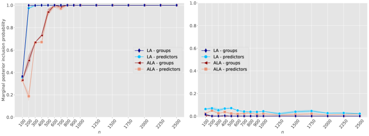
Figure 1: Comparison of ALA and LA for posterior inclusion probabilities of groups and predictors when $n$ varies from 100 to $2,500$, with $p=50$. Left: average posterior inclusion probabilities for truly active variables. Right: average posterior inclusion for truly inactive variables.

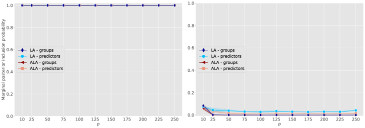
Figure 2: Comparison of ALA and LA for posterior inclusion probabilities of groups and predictors when $p$ varies from 10 to 25, with $n=1,500$. Left: average posterior inclusion probabilities for truly active variables. Right: average posterior inclusion for truly inactive variables.

Figure 1 summarizes the results from the first scenario. Both LA and ALA discriminate properly truly active from inactive groups and variables when $n$ is large enough. However, LA assigns larger inclusion probabilities for truly variables when $n\leq 500$. Figure 2 summarizes the results for the $n=1,500$ case, when $p$ varies from 10 to 25. LA and ALA performed equally and provided accurate estimates both for groups and variables.

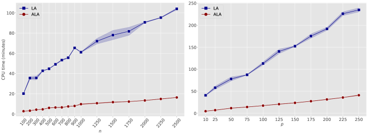
Figure 3: Comparison of ALA and LA for run time of waste-free SMC. Left: average run time when $n$ varies from 100 to $2,500$ ($p=50$). Right: average run time when $p$ varies from 10 to $25$ ($n=1,500$).

Figure 3 compares the performance of ALA and LA in terms of computation time in both scenarios. ALA significantly reduces run times compared to LA, especially for larger $n$ (mean run time = 16 min for ALA vs. 102 min for LA when $n=2,500$ and $p=50$) and $p$ (mean run time = 39 min for ALA vs. 330 min for LA when $p=250$ and $n=1,500$). It is interesting to note that the CPU time still grows with $n$ with ALA, although the computation of ALA is independent of $n$. The likely explanation is that when $n$ grows, the prior and the posterior differ more markedly, and thus more intermediate tempering distributions are required to bridge between the two. Still, the dependence on $n$ of the CPU time remains mild compared to the LA-based sampler.

To sum up, one observes that ALA considerably reduces the CPU time of the sampler, in particular for large $n$ (sample size) and $p$ (number of variables). In return, as expected ALA tends to under-estimate the probability of inclusion of active variables, at least for $n$ not sufficiently large.

4.2 Bi-level selection on the French National Healthcare Insurance database

To examine the performance of our SMC sampler on a big dataset, we study which factors are associated to sudden cardiac death (SCD) in a French epidemiological study. Sudden cardiac death is an unexpected death due to cardiac causes that occurs in a short time period (generally within 1 hour of symptom onset) in a person with known or unknown cardiac disease. Despite progress in epidemiology, clinical profiling and interventions, it remains a major public health problem worldwide, accounting for 10 to 20% of deaths in industrialised countries. The annual incidence of SCD is estimated 180,000 to 450,000 in the United States (Melissa et al., (2011)) and 275,000 in Europe (Empana et al., (2022)). The prognosis is terrible, with less than 10% surviving to hospital discharge, and significant functional and cognitive disabilities often persist among those who survive (Bougouin et al., (2014)). Therefore, identification of persons with an elevated risk of SCD is highly relevant from a clinical and public health perspective.

In this study, we implement bi-level variable selection to identify outpatient drugs and hospital diagnoses that could help to enhance risk prediction performance of SCD over many potential risk factors collected from electronic health records. We analyse the medical trajectories of $n_{\mathrm{cases}}=23,958$ cases of SCD collected between 2016 and 2020 throughout the Paris Sudden Death Expertise Center (Bougouin et al., (2014)), and $n_{\mathrm{controls}}=23,958$ controls sampled from the French general population. Cases and controls were matched with age, sex and residence area.

For the $n=n_{\mathrm{cases}}+n_{\mathrm{controls}}=47,916$ individuals, we collected data from the French National Health Insurance (SNDS) database, which manages all reimbursements of healthcare for people affiliated to a health insurance scheme in France. It provides information on all healthcare expenses, on an individual level, including visits, procedures and reimbursed drugs relative to outpatient medical care claims, information from hospital discharge summaries and chronic conditions. Data acquisition is permanent, from birth to death, irrespective of wealth, age, or work status, resulting in one of the largest electronic health records databases in the world. The SNDS database has been described in detail previously and has been used to conduct multiple studies in cardiovascular epidemiology (Olivier et al., (2022)). More details are available at https://www.health-data-hub.fr/.

We collected all outpatient drugs and hospital diagnoses that occurred up to 5 years before SCD; in this way we obtained $q=36$ groups and $p=337$ binary variables (0/1 whether the individual took a particular drug in the last 5 years, or a drug in the corresponding group). In the 36 groups, the minimum number of variables observed is 2 and the maximum is 27. No external variables were included in the study ($r=0$). Figures 4 and 5 summarise the results of our ALA-based SMC sampler in terms of variable (and group) selection. We evaluate groups and variables selected by our model by comparing them with those described in the medical literature related to SCD. Overall, 16 out of 36 groups and 55 out of 337 variables are selected (Figure 4). Our bi-level variable selection scheme allows for a more flexible structure than "all-in all-out" methods and identifies 3 different "clusters" represented in Figure 5.

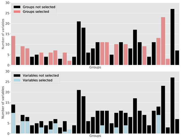
Figure 4: Groups and predictors selected by the ALA-based SMC sampler. Top: selection of groups. Bottom: selection of predictors.

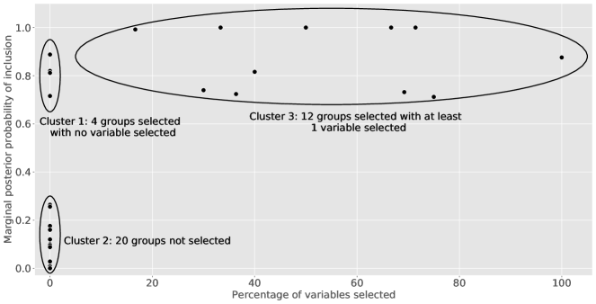
Figure 5: Bi-level variable selection scheme proposed by the ALA-based SMC sampler

In the first cluster (located in the upper left corner), 4 groups of hospital diagnoses are selected without any variable included. These groups correspond to diseases of the eye ($\pi(\gamma_{k}=1)=0.82$), diagnoses related to pregnancy, childbirth and the puerperium ($\pi(\gamma_{k}=1)=0.82$), injury and poisoning ($\pi(\gamma_{k}=1)=0.72$) and diagnoses for other special purposes ($\pi(\gamma_{k}=1)=0.89$). They are selected with high marginal posterior probabilities of inclusion, although none of their 46 corresponding variables are selected. This result suggests therefore that only global relationships exist between these groups and SCD, with no any precise effect of diseases or treatments.

In the second cluster (located in the lower left corner), 20 groups are not selected, as well as their 189 corresponding variables. They include diverse subgroups of diseases and treatments.

In the third cluster (located in the upper right corner), 12 groups are selected with at least 1 variable included. Among them, 3 well known groups of risk factors of SCD are identified. First, diseases and drugs associated to the cardiovascular system are selected (with $\pi(\gamma_{k}=1)=0.74$ and $\pi(\gamma_{k}=1)=1$ respectively), including 9 out of 19 variables. This result was expected, as cardiovascular conditions are known to be the most common pathology under SCD. Second, diseases and drugs related to the nervous system are selected (with $\pi(\gamma_{k}=1)=0.72$ and $\pi(\gamma_{k}=1)=1$ respectively), including 9 out of 18 variables. Several studies have suggested relationships between diseases of the nervous system and SCD (Japundzic-Zigon et al., (2018)). Indeed, some neurological disorders can cause damage to the heart and blood vessels (such as stroke or brain injury) or arrhythmia (such as epilepsy), increasing the risk of SCD. There are also neurological conditions that can cause SCD directly, such as long QT or Brugada syndromes, which affect the electrical activity of the heart. Third, a group related to treatments of the respiratory system is selected. A number of studies have also addressed the relationship between respiratory disorders and SCD. In particular, cumulating evidence associates chronic obstructive pulmonary diseases with an increased risk of SCD both in cardiovascular patient groups and in community-based studies, independent of cardiovascular risk profile (Van den Berg et al., (2016)).

We ran our ALA-based SMC samplers 10 times to assess its numerical stability. Figure 6 describes the interquartile range of the marginal posterior probabilities of inclusion for variables. The mean run time was 61.8 hours (totalling to 7 days of total CPU time). We also launched 10 executions of our LA-based SMC sampler, but these executions had not completed after 30 days. We can see that, for this particular dataset, using ALA becomes crucial to make the approach usable for practitioners.

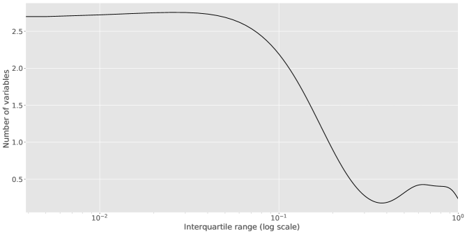
Figure 6: Kernel density estimate of the interquartile range (log scale) of the marginal posterior inclusion probabilities (variables) for the ALA-based SMC sampler.

5 Conclusion

Our bi-level variable selection approach based on a waste-free SMC sampler and the ALA approximation offers reliable performance for large-scale datasets within a reasonable computation time. Furthermore, our approach is more flexible than most of existing schemes, which impose only “all-in” or “all-out” selection for variables in the same group. This work could be therefore helpful in a wide range of applications, such as biomedical studies, where standard approaches provide information which may be difficult for physicians to interpret.

References

- Bougouin et al., (2014) Bougouin, W., Lamhaut, L., Marijon, E., Jost, D., Dumas, F., Deye, N., Beganton, F., Empana, J.-P., Chazelle, E., Cariou, A., and Jouven, X. (2014). Characteristics and prognosis of sudden cardiac death in greater Paris: population-based approach from the Paris sudden death expertise center (Paris-sdec). Intensive Care Medicine, 40(6):846–854.
- Cai et al., (2020) Cai, M., Dai, M., Ming, J., Peng, H., Liu, J., and Yang, C. (2020). BIVAS: a scalable Bayesian method for bi-level variable selection with applications. J. Comput. Graph. Statist., 29(1):40–52.
- Chen et al., (2016) Chen, R.-B., Chu, C.-H., Yuan, S., and Wu, Y. N. (2016). Bayesian sparse group selection. J. Comput. Graph. Statist., 25(3):665–683.
- Dau and Chopin, (2022) Dau, H.-D. and Chopin, N. (2022). Waste-free sequential Monte carlo. Journal of the Royal Statistical Society: Series B (Statistical Methodology), 84(1):114–148.
- Empana et al., (2022) Empana, J.-P., Lerner, I., Valentin, E., Folke, F., Böttiger, B., Gislason, G., Martin, J., Ringh, M., Beganton, F., Bougouin, W., Eloi, M., Blom, M., Tan, H., and Jouven, X. (2022). Incidence of sudden cardiac death in the European union. Journal of the American College of Cardiology, 79(18):1818–1827.
- Japundzic-Zigon et al., (2018) Japundzic-Zigon, N., Sarenac, O., Lozic, M., Vasic, M., Tasic, T., Bajic, D., Kanjuh, V., and Murphy, D. (2018). Sudden death: Neurogenic causes, prediction and prevention. European Journal of Preventive Cardiology, 25(1):29–39.
- Mallick and Yi, (2017) Mallick, H. and Yi, N. (2017). Bayesian group bridge for bi-level variable selection. Comput. Statist. Data Anal., 110:115–133.
- Melissa et al., (2011) Melissa, K., Gregg, F., Eric, P., Anne, C., Adrian, H., Gillian, S., Kevin, T., David, H., and Sana, A.-K. (2011). Systematic review of the incidence of sudden cardiac death in the united states. Journal of the American College of Cardiology, 57(7):794–801.
- Olivier et al., (2022) Olivier, P., Pascal, D., Lortet-Tieulent, Joannie, Jean-Claude, D., Julien, B., Alexandre, V., Claire, L., Eloi, M., and Serge, B. (2022). Healthcare costs in implantable cardioverter-defibrillator recipients: A real-life cohort study on 19,408 patients from the French national healthcare database. International Journal of Cardiology, 348:39–44.
- Rossell et al., (2021) Rossell, D., Abril, O., and Bhattacharya, A. (2021). Approximate Laplace approximations for scalable model selection. J. R. Stat. Soc. Ser. B. Stat. Methodol., 83(4):853–879.
- Schäfer, (2012) Schäfer, C. (2012). Monte Carlo methods for sampling high-dimensional binary vectors. PhD thesis, Université Paris Dauphine.