Indoor experimental validation of MPC-based trajectory tracking
for a quadcopter via a flat mapping approach

Abstract

Differential flatness has been used to provide diffeomorphic transformations for non-linear dynamics to become a linear controllable system. This greatly simplifies the control synthesis since in the flat output space, the dynamics appear in canonical form (as chains of integrators). The caveat is that mapping from the original to the flat output space often leads to nonlinear constraints. In particular, the alteration of the feasible input set greatly hinders the subsequent calculations. In this paper, we particularize the problem for the case of the quadcopter dynamics and investigate the deformed input constraint set. An optimization-based procedure will achieve a non-conservative, linear, inner-approximation of the non-convex, flat-output derived, input constraints. Consequently, a receding horizon problem (linear in the flat output space) is easily solved and, via the inverse flat mapping, provides a feasible input to the original, nonlinear, dynamics. Experimental validation and comparisons confirm the benefits of the proposed approach and show promise for other class of flat systems.

I Introduction

In the context of the global contagious pandemic in recent years, multicopters, have received remarkable attention thanks to their mobility and a wide range of applications in transportation and delivery. Although these systems have been analyzed for decades [1, 2], the question of optimally improving the tracking performance is still open due to their strong nonlinearity and the presence of physical constraints.

To tackle the issue, while several approaches have been proposed [1, 2, 3], we focus our attention on Model Predictive Control (MPC) since it has the ability of computing the optimal control inputs while ensuring constraint satisfaction. In the literature, there are various strategies for implementing MPC in real-time with multicopters. For example, one option is to directly consider the nonlinear dynamics and design a nonlinear controller [3]. However, in practice, solving a nonlinear optimization problem requires a high computation power. Thus, apart from applying MPC in a nonlinear setting, the dynamics is usually governed by exploiting its model inversion given by the theory of differentially flat systems [4]. Indeed, the quadcopter system is famously known to accept a special representation through differential flatness (i.e., all its states and inputs are algebraically expressed in terms of a flat output and a finite number of its derivatives). Based on such property, on one hand, one method is to exploit that flat representation to construct an integral curve (a solution of the system’s differential equation) by parameterizing the flat output in time with sufficient smoothness. Then, along such curve, the dynamics are approximated by linear time varying models and controlled with linear MPC [5]. Expectedly, this method provides a computational advantage thanks to the approximated linear model while the convexity of the input constraint is preserved. Yet, one shortcoming is that the model relies on an approximation, leading to the sensitivity of the controller to uncertainties. On the other hand, in the context of exact linearization, the nonlinear dynamics can be linearized in closed-loop using a linearization law taken from the relation between the flat output and the inputs [3, 6], making the stability more straightforward to analyze. However, the drawback is that, during the linear control design in the new coordinates, the constraint set will be altered, leading to a nonlinear or even non-convex set. This phenomenon is often dealt by online prediction, conservative offline approximation [3, 7] or constraint satisfying feedforward reference trajectory.

This paper addresses the challenges and benefits of synthesizing a controller within the flat output space of a multicopter. Since in the new space coordinates, the input constraints are convoluted, we formulate a zonotope-based inner approximation of the constraints. Then a classical MPC for the linearized system is employed, which shows good performances in practice. Briefly, our main contributions are:

• describe and investigate the system’s constraints in the new coordinates deduced from its flatness properties;

• propose an optimization-based procedure to find a maximum inscribed inner approximation of the aforementioned altered constraint set by adopting the technique of rescaling zonotopes [8];

• construct an MPC scheme for the multicopter linear dynamics and experimentally validate it with the Crazyflie 2.1 platform in comparison with the piece-wise affine approach [5] and other existing results in the literature.

The remainder of the paper is structured as follows. Section II presents the system’s dynamics together with its input sets, both before and after the closed-loop linearization via flatness. Exploiting the convexity of the new constraints, we provide a zonotopic-based approximation procedure in Section III. The effectiveness of our approach is then experimentally validated in Section IV. Finally, Section V draws the conclusion and discusses future directions.

Notation: Bold capital letters refers to the matrices with appropriate dimension. $\boldsymbol{I}_{n}$ and $\boldsymbol{0}_{n}$ denote the identity and zero matrix of dimension $(n\times n)$, respectively. Vectors are represented by bold letters. $\text{diag}(\cdot)$ denotes the diagonal matrix created by the employed components. $\|\boldsymbol{x}\|_{\boldsymbol{Q}}\triangleq\sqrt{\boldsymbol{x}^{\top}\boldsymbol{Q}\boldsymbol{x}}$. For discrete system, $\boldsymbol{x}_{k}$ denotes the value of $\boldsymbol{x}$ at time step $k$. The superscript “$\mathrm{ref}$” represents the reference signal (e.g, $\boldsymbol{x}^{\mathrm{ref}}$). Next, $\mathcal{N}_{m}\triangleq\{1,...,m\}$ denotes the set of integers $i$ such that $1\leq i\leq m$. Furthermore, $\partial\mathcal{X}$ and $\text{int}(\mathcal{X})$ respectively denote the boundary and the interior of the set $\mathcal{X}$. Finally, $\text{Conv}\{\cdot\}$ denotes the convex hull operation.

II System description and input constraints formulation in the flat output space

In this section, we briefly present the quadcopter model together with its flat characterization. Next, due to the variable change, the input constraint of the quadcopter is transformed into a different non-convex set which then is replaced by a convex alternative.

II-A Flat characterization of quadcopter model

Let us recall the quadcopter translational dynamics:

$$\begin{bmatrix}\ddot{x}\\ \ddot{y}\\ \ddot{z}\end{bmatrix} \text{=}\begin{bmatrix}T(\cos\phi\sin\theta\cos\psi\text{+}\sin\phi\sin\psi)\\ T(\cos\phi\sin\theta\sin\psi{-}\sin\phi\cos\psi)\\ T\cos\phi\cos\theta-g\end{bmatrix}\text{= }\boldsymbol{h}_{\psi}(\boldsymbol{u}),$$ (1)

where $x,\,y,\,z$ are the positions of the drone, $\psi$ denotes the yaw angle, $g$ is the gravity acceleration and $\boldsymbol{u}=[T\,\;\phi\,\;\theta]^{\top}\in\mathbb{R}^{3}$ collects the inputs including the normalized thrust, roll and pitch angle, respectively. Finally, $\mathcal{U}$ denotes the input constraint set, which is described as:

$$\mathcal{U}=\{\boldsymbol{u}:0\leq T\leq T_{max},\;|\phi|\leq\phi_{max},\;|\theta|\leq\theta_{max}\}$$ (2)

where $T_{max}$ and $\theta_{max},\phi_{max}\in(0;{\pi}/{2})$ are, respectively, the upper bound of $T$ and $|\phi|,|\theta|$.

To compensate the system’s nonlinearity, one typical solution is to construct its flat representation [4], i.e, parameterizing all the system’s variables with a special output, called the flat output, and its derivatives. Then, based on such model inversion, one can define a coordinate change associated with a dynamic feedback linearizing the system in closed-loop. Indeed, this quadcopter model is known to be differentially flat, and its flat representation can be expressed as[9]:

$$T =\sqrt{\ddot{\sigma}_{1}^{2}+\ddot{\sigma}_{2}^{2}+(\ddot{\sigma}_{3}+g)^{2}},$$ (3a)

$$\phi =\arcsin{\left({(\ddot{\sigma}_{1}\sin{\psi}-\ddot{\sigma}_{2}\cos{\psi})}/{T}\right)},$$ (3b)

$$\theta =\arctan{\left({(\ddot{\sigma}_{1}\cos{\psi}+\ddot{\sigma}_{2}\sin{\psi})}/{(\ddot{\sigma}_{3}+g)}\right)},$$ (3c)

with the flat output $\boldsymbol{\sigma}=[\sigma_{1},\sigma_{2},\sigma_{3}]^{\top}\triangleq[x\,\,y\,\,z]^{\top}$.

Next, by exploiting (3a)-(3c), we employ an input transformation which is compactly written as $\boldsymbol{u}=\boldsymbol{\varphi}_{\psi}(\boldsymbol{v})$ and detailed in (4). In the mapping, $\boldsymbol{v}=[v_{1},v_{2},v_{3}]^{\top}$ collects the input the new coordinates called the flat output space.

$$T =\sqrt{v_{1}^{2}+v_{2}^{2}+(v_{3}+g)^{2}},$$ (4a)

$$\phi =\arcsin{\left({(v_{1}\sin{\psi}-v_{2}\cos{\psi})}/{T}\right)},$$ (4b)

$$\theta =\arctan{\left({(v_{1}\cos{\psi}+v_{2}\sin{\psi})}/{(v_{3}+g)}\right)}.$$ (4c)

Then, under the condition of $v_{3}\geq-g$ and the mapping (4), the system (1) is transformed into:

$$\ddot{\boldsymbol{\sigma}}=\boldsymbol{v},\text{ with }\boldsymbol{\sigma},\boldsymbol{v}\in\mathbb{R}^{3}.$$ (5)

Ideally, without constraints, the system can be controlled by closing the loop for the trivial system (5). However, as a consequence of the input mapping (4), the constraint $\mathcal{U}$ in (2) becomes geometrically altered. Hence, it is of importance to analyze the alternation to construct a suitable controller. Indeed, hereinafter, we pave the way towards the flatness-based MPC (FB-MPC) design for the linear system (5) by constructing the constraint set for $\boldsymbol{v}$ in the new space.

A general overview of the proposed control scheme for quadcopter control is in Fig. 1. With the reference deduced from the parameterization of the flat output and the feedback signal, the FB-MPC controller computes the necessary input $\boldsymbol{v}$ to compensate the error based on the linear model (5) and the input constraint set in the flat output space. Then the new input $\boldsymbol{v}$ will be mapped back to the original coordinates as $\boldsymbol{u}$ using the transformation (4). Finally, the control $\boldsymbol{u}$ is sent to the drone, ensuring the tracking performance.

Figure 1: Flatness-based MPC control scheme.

II-B Input constraint characterization in the flat output space

As aforesaid, the constraint set $\mathcal{U}$ is complicated by means of (4). Let us denote the new constraint set for $\boldsymbol{v}$ as:

$$\mathcal{V}=\left\{\boldsymbol{v}\in\mathbb{R}^{3}\;|\;\boldsymbol{\varphi}_{\psi}(\boldsymbol{v})\in\mathcal{U}\text{ as in \eqref{eq:orginal_input_constr}}\right\}.$$ (6)

Remark 1

It is essential to point out that our motivation to construct such a set lies on the structural property of the mapping $\boldsymbol{\varphi}^{-1}_{\psi}(\boldsymbol{u})$. Indeed, since the function $\boldsymbol{\varphi}_{\psi}(\boldsymbol{v})$ is continuous and continuously invertible ($\boldsymbol{\varphi}^{-1}_{\psi}(\boldsymbol{u})=\boldsymbol{h}_{\psi}(\boldsymbol{u})$), it describes a homeomorphism which maps the interior and boundary of a set, respectively, to those of its image. Hence, under this mapping, some geometrical properties of $\mathcal{U}$ (e.g, compactness and connectedness) are preserved in $\mathcal{V}$, encouraging us for a later-mentioned approximation.

Regardless, it can be shown that $\mathcal{V}$ in (6) is non-convex: the two vectors $\boldsymbol{v}_{\pm}=\boldsymbol{h}_{\psi}([T_{max},\pm\phi_{max},\pm\theta_{max}]^{\top})\in\mathcal{V}$ but $(\boldsymbol{v}_{+}+\boldsymbol{v}_{-})/2\notin\mathcal{V}$. Moreover, $\mathcal{V}$ appears to be impractical owing to its dependence on the yaw angle $\psi$, which in real applications, is certainly time-variant. For these reasons, let us consider the following subset of $\mathcal{V}$, denoted as $\tilde{\mathcal{V}}$:

$$\tilde{\mathcal{V}}\triangleq\Big{\{}\boldsymbol{v}\in\mathbb{R}^{3}:\begin{bmatrix}{v_{1}^{2}+v_{2}^{2}+(v_{3}+g)^{2}}-T_{max}^{2}\\ v_{1}^{2}+v_{2}^{2}-(v_{3}^{2}+g)^{2}\tan^{2}\epsilon_{max}\end{bmatrix}\leq 0,$$ (7)

$$\epsilon_{max}\triangleq\min(\theta_{max},\phi_{max})\text{ and }v_{3}\geq-g\Big{\}}.$$

Proposition 1

$\tilde{\mathcal{V}}$ in (7) is convex and $\tilde{\mathcal{V}}\subset{\mathcal{V}}$ as in (6).

Proof:

First, to show that $\tilde{\mathcal{V}}\subset{\mathcal{V}}$, from (4), by using Cauchy-Schwarz inequality, we can construct the upper bounds for the roll and pitch angles $\phi,\theta$ as follows [9]:

$$|\sin\phi|\leq\sqrt{{(v_{1}^{2}+v_{2}^{2})}/{\left(v_{1}^{2}+v_{2}^{2}+(v_{3}+g)^{2}\right)}},$$ (8a)

$$|\tan\theta|\leq\sqrt{{(v_{1}^{2}+v_{2}^{2})}/{(v_{3}+g)^{2}}}.$$ (8b)

After some trigonometric transformations, we can see that the right-hand side of both (8a) and (8b) represent the same angle: $\epsilon_{0}(\boldsymbol{v})\triangleq\arctan\sqrt{{(v_{1}^{2}+v_{2}^{2})}/(v_{3}+g)^{2}}$. Hence, (8b) yields: $|\sin\phi|\leq\sin{\epsilon_{0}(\boldsymbol{v})}\text{ and }|\tan\theta|\leq\tan{\epsilon_{0}(\boldsymbol{v})}.$ Then, with $|\phi|,|\theta|<\pi/2$ as in (2) and by imposing $\epsilon_{0}(\boldsymbol{v})\leq\epsilon_{max}$, we have $(|\phi|,|\theta|)\leq(\theta_{max},\phi_{max})$. Thus, if $\boldsymbol{v}\in\tilde{\mathcal{V}}$, $\boldsymbol{v}\in{\mathcal{V}}$. Moreover, the convexity of $\tilde{\mathcal{V}}$ can be shown by analyzing the intersection of the two convex sets: a ball of radius $T_{max}$ and a convex cone defined by the two inequalities $v_{1}^{2}+v_{2}^{2}-(v_{3}^{2}+g)^{2}\tan^{2}\epsilon_{max}\leq 0$, $v_{3}\geq-g$ (see Fig. 2). ∎

Up to this point, the constrained control problem is reduced to governing the linear system (5), under the convex constraints $\boldsymbol{v}\in\tilde{\mathcal{V}}$ as in (7), depicted in Fig. 2. However, to exploit more the advantage of this linear dynamics, it would be computationally beneficial if $\tilde{\mathcal{V}}$ can be approximated by linear constraints, hence, reducing the complexity of the control problem. Thus, in the next section, by parameterizing a family of zonotopes, an optimization problem will be introduced to achieve a tractable representation for $\tilde{\mathcal{V}}$.

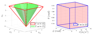
Figure 2: Constraint sets for the input $\boldsymbol{v}$ in the flat output space (left) and the constraint set $\mathcal{U}$ in the original space (right).

III Input constraints approximation
in the flat output space

With the idea of approximating the set by inflating a geometric object and achieve the largest volume inscribed, ellipsoids are typically employed owing to their volume’s explicit expression[10]. However, with ellipsoids, few advantages can be of use both geometrically and computationally if employed with MPC. Hence, let us exploit the benefits of zonotopes for which we not only have the volume’s explicit formula but also obtain linear constraints.

III-A Zonotope parameterization

Let us first recall the definition of a zonotope.

Definition 1

In $\mathbb{R}^{d}$, given a center point $\boldsymbol{c}$ and a set of $n_{g}$ vectors $\{\boldsymbol{g}_{1},...,\boldsymbol{g}_{n_{g}}\}$, then $\mathcal{Z}(\boldsymbol{G},\boldsymbol{c})$ is called a zonotope and can be described as [11]:

$$\mathcal{Z}(\boldsymbol{G},\boldsymbol{c})=\{\boldsymbol{c}+\textstyle\sum_{i=1}^{n_{g}}\beta_{i}\boldsymbol{g}_{i}:|\beta_{i}|\leq 1\},$$ (9)

with $\boldsymbol{G}=[\boldsymbol{g}_{1},\boldsymbol{g}_{2},...,\boldsymbol{g}_{n_{g}}]$ gathering all the generators $\boldsymbol{g}_{i}$. A zonotope is, indeed, a centrally symmetric polytope.

Additionally, the following properties can be established. Consider the following set $\mathbf{E}(\mathcal{Z}(\boldsymbol{G},\boldsymbol{c}))$ defined as:

$$\mathbf{E}(\mathcal{Z}(\boldsymbol{G},\boldsymbol{c}))\triangleq\big{\{}\boldsymbol{c}+\textstyle\sum_{i=1}^{n_{g}}\alpha_{i}\boldsymbol{g}_{i},|\alpha_{i}|=1\big{\}}.$$ (10)

Then, the set $\mathbf{E}(\mathcal{Z}(\boldsymbol{G},\boldsymbol{c}))$ in (10) is a finite subset of $\mathcal{Z}(\boldsymbol{G},\boldsymbol{c})$ and contains all of its vertices [11]. Consequently, for a convex set $\mathcal{X}$, the inclusion $\mathcal{Z}(\boldsymbol{G},\boldsymbol{c})\subseteq\mathcal{X}$ holds if and only if $\mathbf{E}(\mathcal{Z}(\boldsymbol{G},\boldsymbol{c}))\subset\mathcal{X}$. Furthermore, as proposed in [8], consider a family of parameterized zonotopes:

$$\mathcal{Z}(\boldsymbol{G}\Delta,\boldsymbol{c})=\{\boldsymbol{c}+\textstyle\sum_{i=1}^{n_{g}}\beta_{i}\delta_{i}\boldsymbol{g}_{i}:|\beta_{i}|\leq 1\},$$ (11)

where $\boldsymbol{G}$ is a given generator matrix and $\Delta=\text{diag}(\boldsymbol{\delta})$ denotes a diagonal matrix whose diagonal is collected in $\boldsymbol{\delta}=[\delta_{1},...,\delta_{n_{g}}]$. Then, its volume is explicitly written as:

$$\mathcal{C}(\boldsymbol{\delta})=\sum_{1\leq k_{1}<...<k_{d}\leq n_{g}}\left|\det(\boldsymbol{G}^{k_{1}...k_{d}})\right|\;\;\;\,\prod_{\mathclap{{k\in\{k_{1},...,k_{d}\}}}}\delta_{k}$$ (12)

where $\boldsymbol{G}^{k_{1}...k_{d}}\in\mathbb{R}^{d\times d}$ denotes the matrix formed by stacking the $k_{l}$-th column, $l\in\mathcal{N}_{d}$, of $\boldsymbol{G}$ together.

Using the above tools, we propose in the next subsection a zonotopic inner-approximation for the set $\tilde{\mathcal{V}}$ in (7).

III-B Constraints approximation in the flat output space

In here, we construct an optimization problem to find the largest zonotope from the family of $\mathcal{Z}(\boldsymbol{G}\Delta,\boldsymbol{c})$ as in (11) constrained in the convex set $\tilde{\mathcal{V}}\subset\mathbb{R}^{3}$:

$$(\boldsymbol{\delta},\boldsymbol{c})^{*}=\underset{\boldsymbol{\delta},\boldsymbol{c}}{\arg\operatorname{max}}\;\mathcal{C}(\boldsymbol{\delta}),$$ (13a)

s.t $$\boldsymbol{v}\in\tilde{\mathcal{V}},\forall\boldsymbol{v}\in\mathbf{E}(\mathcal{Z}(\boldsymbol{G}\Delta,\boldsymbol{c})),$$ (13b)

$$\boldsymbol{v}^{\mathrm{int}}\in\mathcal{Z}(\boldsymbol{G}\Delta,\boldsymbol{c}),$$ (13c)

where $\mathcal{Z}(\boldsymbol{G},\boldsymbol{c})\subset\mathbb{R}^{3}$ denotes the zonotope formed by the given $n_{g}$ generators in $\boldsymbol{G}\in\mathbb{R}^{3\times n_{g}}$ centered at $\boldsymbol{c}$; $\boldsymbol{\delta}=[\delta_{1},...,\delta_{n_{g}}]\in\mathbb{R}^{n_{g}}$ is a scaling factor magnifying the original zonotope $\mathcal{Z}(\boldsymbol{G},\boldsymbol{c})$. $\mathcal{C}(\boldsymbol{\delta})$ denotes the volume of $\mathcal{Z}(\boldsymbol{G}\Delta,\boldsymbol{c})$ computed as in (12) with $\Delta\triangleq\text{diag}(\boldsymbol{\delta})$. Next, $\mathbf{E}(\mathcal{Z}(\boldsymbol{G}\Delta,\boldsymbol{c}))\subset\mathcal{Z}(\boldsymbol{G}\Delta,\boldsymbol{c})$ is finite and contains all vertices of $\mathcal{Z}(\boldsymbol{G}\Delta,\boldsymbol{c})$, and can be enumerated as in (10). This condition (13b) ensures the inclusion $\mathcal{Z}(\boldsymbol{G}\Delta,\boldsymbol{c})\subset\tilde{\mathcal{V}}$ as previously discussed. Finally, $\boldsymbol{v}^{\mathrm{int}}\in\mathrm{int}(\tilde{\mathcal{V}})$ is a user-defined point towards which the resulting set is allowed to expand. Specifically, since zonotopes are symmetric, it is impossible for them to expand freely inside $\tilde{\mathcal{V}}$. Therefore, progressively imposing the condition (13c) with different $\boldsymbol{v}^{\mathrm{int}}$ helps us obtain several zonotopes reaching to specific “corners” of $\tilde{\mathcal{V}}$. Then the final approximated set is achieved as the convex hull of all the zonotopes deduced from those choices of $\boldsymbol{v}^{\mathrm{int}}$.

For instance, let us denote $\mathcal{I}$ the sets of choice containing some $\boldsymbol{v}^{\mathrm{int}}\in\text{int}(\tilde{\mathcal{V}})$. One candidate can be enumerated as in (14) which contains $N_{0}+1$ points taken between two extreme ones of $\tilde{\mathcal{V}}$: $[0,0,-g]^{\top}$ and $[0,0,T_{max}-g]^{\top}$:

$$\mathcal{I}=\{\boldsymbol{v}^{\mathrm{int}}_{0},...,\boldsymbol{v}^{\mathrm{int}}_{N_{0}}\}$$ (14)

with $\boldsymbol{v}^{\mathrm{int}}_{k}=[0,0,1]^{\top}((1-{k}/{N_{0}})T_{max}-g)$. Then, for each $0\leq k\leq N_{0}$ as in (14), we obtain from (13) a parameterized zonotope $\mathcal{Z}(\boldsymbol{G}\Delta,\boldsymbol{c})$, assigned as $\mathcal{S}_{v}^{k}$. Finally, the resulting approximation set is computed as:

$$\mathcal{S}_{v}=\text{Conv}\left\{\mathcal{S}_{v}^{0},...,\mathcal{S}_{v}^{N_{0}}\right\}.$$ (15)

The procedure is summarized in Algorithm 1.

Input: Generator $\boldsymbol{G}$ as in (13) and $\mathcal{I}$ as in (14).

Output: The approximation set $\mathcal{S}_{v}$ as in (15) of $\tilde{\mathcal{V}}$.

for $k=0$ to $N_{0}$  do

       $\boldsymbol{v}^{\mathrm{int}}_{k}\leftarrow[0,0,1]^{\top}((1-{k}/{N_{0}})T_{max}-g)$;

       Solve the optimization problem (13) for $(\boldsymbol{\delta},\boldsymbol{c})$;

       $\mathcal{S}_{v}^{k}\leftarrow\mathcal{Z}(\boldsymbol{G}\Delta,\boldsymbol{c})$ with $\Delta=\text{diag}(\boldsymbol{\delta})$;

      

end for

$\mathcal{S}_{v}\leftarrow\text{Conv}\left\{\mathcal{S}_{v}^{0},...,\mathcal{S}_{v}^{N_{0}}\right\}$ as in (15).

Algorithm 1 $\tilde{\mathcal{V}}$ approximation procedure.

Remark 2

Although the semi-definite condition (13b) is straightforward to construct, it comes with a shortcoming: the computational cost rises exponentially with the number of generators, $n_{g}$, since the number of elements in $\mathbf{E}(\mathcal{Z}(\boldsymbol{G}\Delta,\boldsymbol{c}))$ is $2^{n_{g}}$. This drawback is indeed burdensome, especially for the approximation of high dimensional sets, because one needs a sufficiently large number of generators to have a good basis zonotope $\mathcal{Z}(\boldsymbol{G},\boldsymbol{c})$ to be scaled with $\boldsymbol{\delta}$.

III-C Simulation result

In this part, we discuss the simulation result of applying Algorithm 1 for $\tilde{\mathcal{V}}$ as in (7) with $\mathcal{I}$ enumerated as in (14). For illustration, we examine two scenarios with $N_{0}=2$ and $N_{0}=25$ for (14). The result, its specification and parameters setup are provided in Fig. 3 and Table I, respectively.

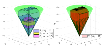
Figure 3: Approximated constraint sets for the new input $\boldsymbol{v}$.

TABLE I: Parameters setup for $\tilde{\mathcal{V}}$ approximation

Symbols	Values
$g$, $T_{max}$	9.81; 19.62 $m/s^{2}$
$\theta_{max},\phi_{max}$	0.1745 $rad$ $(10^{o})$
$\boldsymbol{G}$	$\begin{bmatrix}1&0&0&0&0\\ 0&1&0&1&-1\\ 0&0&1&2&2\end{bmatrix}$
$\bar{v}_{1p}=\bar{v}_{2p}=\bar{v}_{3p}$	1.0875
$[\bar{v}_{1b},\bar{v}_{2b},\bar{v}_{3b}]$	$[0.815,0.815,3.270]$

For comparison, we examine other constraint sets for quadcopter in the literature, which are constructed as follows.

• In [3], a box-type subset of $\tilde{\mathcal{V}}$ was introduced as:

  $$\mathcal{P}_{v}=\{\boldsymbol{v}\in\mathbb{R}^{3}:|v_{i}|\leq\bar{v}_{ip},i\in\{1,2,3\}\}$$ (16)

  with the constant $\bar{v}_{ip}$ satisfying the conditions:

  $$\begin{cases}\bar{v}_{3p}<g;\,\bar{v}_{1p}^{2}+\bar{v}_{2p}^{2}\leq(-\bar{v}_{3p}+g)^{2}\tan^{2}\epsilon_{max}&\\ \sqrt{\bar{v}_{1p}^{2}+\bar{v}_{2p}^{2}+(\bar{v}_{3p}+g)^{2}}\leq T_{max}.&\end{cases}$$

• The approximated origin-centered constraint set, in [7, 6], described as:

  $$\mathcal{B}_{v}=\{\boldsymbol{v}\in\mathbb{R}^{3}:|v_{i}|\leq\bar{v}_{ib},i\in\{1,2,3\}\}$$ (17)

  can be similarly found by employing (13) with $\boldsymbol{G}=\boldsymbol{I}_{3}$ and $\boldsymbol{v}^{\mathrm{int}}=[0,0,0]^{\top}$.

The illustration of the aforementioned sets are also shown in Fig. 3 with their numerical values given in Table I and II.

TABLE II: Result specifications for $\tilde{\mathcal{V}}$ approximation

	$\mathcal{S}_{v},N_{0}=2$	$\mathcal{S}_{v},N_{0}=25$	$\mathcal{P}_{v}$	$\mathcal{B}_{v}$
Volume	122.57	125.27	10.29	17.39
No. of vertices	28	226	8	8
No. of inequalities	20	216	6	6

As depicted in Fig. 3, our approach provides an improved approximation for the input $\boldsymbol{v}$, with respect to the literature. Prior to this point, the ingredients for an MPC design in the new coordinates are ready. More precisely, the system now can be governed by controlling its image in the flat output space as in (5) with the corresponding input constraint $\mathcal{S}_{v}$ resulted from Algorithm 1. Therefore, next, we validate our results via different tests within the MPC settings.

IV MPC design with experimental validation

To demonstrate the practical viability of our approach, we first present the MPC synthesis utilizing the linear model (5) in the new coordinates, with the corresponding linear constraint set $\mathcal{S}_{v}$ as in (15). The application is conducted using the Crazyflie 2.1 nano-drone with various flight scenarios.

IV-A MPC setup

To embed the model (5) and the constraints $\mathcal{S}_{v}$ in the MPC framework, we first proceed with the discretization as follows. Let $\boldsymbol{\xi}=[\sigma_{1},\sigma_{2},\sigma_{3},\dot{\sigma}_{1},\dot{\sigma}_{2},\dot{\sigma}_{3}]^{\top}$ denotes the state vector of the system (5). Then applying Runge-Kutta (4th order) discretization method to (1) yields:

$$\boldsymbol{\xi}_{k+1}=\boldsymbol{A}\boldsymbol{\xi}_{k}+\boldsymbol{B}\boldsymbol{h}_{\psi}(\boldsymbol{u}_{k})\triangleq\boldsymbol{f}_{d}(\boldsymbol{\xi}_{k},\boldsymbol{u}_{k}),$$ (18)

with $\boldsymbol{A}=\begin{bmatrix}\boldsymbol{I}_{3}&t_{s}\boldsymbol{I}_{3}\\ \boldsymbol{0}_{3}&\boldsymbol{I}_{3}\end{bmatrix}$, $\boldsymbol{B}=[t_{s}^{2}\boldsymbol{I}_{3}/2,\;t_{s}\boldsymbol{I}_{3}]^{\top}$ and the sampling time $t_{s}$. Next, let us introduce the following controllers employed for the validation and comparison.

Flatness-based MPC (FB-MPC): with $\boldsymbol{u}_{k}=\boldsymbol{\varphi}_{\psi}(\boldsymbol{v}_{k})$ as in (4), the system now can be controlled with the linear dynamics: $\boldsymbol{\xi}_{k+1}=\boldsymbol{A}\boldsymbol{\xi}_{k}+\boldsymbol{B}\boldsymbol{v}_{k}$, subject to the new input constraint $\boldsymbol{v}_{k}\in\mathcal{S}_{v}$ (with $N_{0}=2$). We solve the following online problem over the prediction horizon $N_{p}$ steps:

$$\underset{\mathclap{\boldsymbol{v}_{k},{...},\boldsymbol{v}_{k\text{+}N_{p}-1}}}{\arg\min\;\;\;\;\;}\sum_{i=0}^{N_{p}-1}\|\boldsymbol{\xi}_{i+k}-\boldsymbol{\xi}_{i+k}^{\mathrm{ref}}\|_{\boldsymbol{Q}}^{2}+\|\boldsymbol{v}_{i+k}-\boldsymbol{v}_{i+k}^{\mathrm{ref}}\|_{\boldsymbol{R}}^{2}$$ (19)

$$\text{s.t: }\begin{cases}\boldsymbol{\xi}_{i+k+1}=\boldsymbol{A}\boldsymbol{\xi}_{i+k}+\boldsymbol{B}\boldsymbol{v}_{i+k},&\\ \boldsymbol{v}_{i+k}\in{\mathcal{S}_{v}},i\in\{0,...,N_{p}-1\}&\end{cases}\vspace{-0.3cm}$$

with $\boldsymbol{\xi}_{k}^{\mathrm{ref}},\boldsymbol{v}_{k}^{\mathrm{ref}}$ gathering the reference signal of the state $\boldsymbol{\xi}$ and input $\boldsymbol{v}$ at time step $k$. Then the first value of the solution sequence (i.e, $\boldsymbol{v}_{k}$) will be used to compute the real control $\boldsymbol{u}_{k}=\boldsymbol{\varphi}_{\psi}(\boldsymbol{v}_{k})$, which then is applied to the quadcopter.

Piece-Wise Affine MPC (PWA-MPC): For comparison, this method is adopted from [5] with the linearization of the model via Taylor series and the linear MPC setup. Details on the implementation are given in the Appendix.

Remark 3

In the flat output space, by using our convex approximation of the feasible domain, the MPC design employs both a linear model and linear constraints. Hence, within this framework, other properties (e.g, stability, robustness), either in discrete or continuous time, become more accessible for investigation [12, 13]. Note that these advantages do not exist for all flat systems, especially for those with the flat output different from the states (or output) of interest [14, 15], hence, complicating the theoretical guarantees when switching from one space to the other.

IV-B Scenarios of trajectories

To identify benefits and drawbacks of the two methods, we provide some scenarios of trajectories. In those trajectories, the flat output $\boldsymbol{\sigma}$ in (5) will be parameterized in time, which leads to the complete nominal reference of the system thanks to the representation (3). The trajectories are described as:

• Ref. 1: This reference is adopted from [16, 15], with the energetically optimal B-spline parameterized curve (order 8) passing the way-points $w_{k}$ at $t_{k}\,(s)$:

$$w_{k}\in\left\{\begin{aligned} (0;0;3.5);(3;-3;4);(6;0;7.5);&\\ (6;3;8);(3;6;8);(0;6;8);&\\ (-3;3;8);(-3;0;5);(0;0;3.5)&\end{aligned}\right\}\times 10\;(cm)$$

$$t_{k}=(k-1)\times 30/8\,(s),k\in\{1,2,...,9\}.$$

With this method, the curve’s parameters are chosen so that all the states and inputs respect their constraints, giving a favorable reference to them to follow.

• Ref. 2: To make the reference more aggressive, set points are given under sequences of step functions.

• Ref. 3: Next, we adopt the circular trajectory in [6] as:

  $$\sigma_{1\,\mathrm{ref}}(t)=0.5\cos\omega t,\sigma_{2\,\mathrm{ref}}(t)=0.5\sin\omega t$$

  $$\sigma_{3\,\mathrm{ref}}(t)=0.3(m),\omega=0.3\pi.$$

• Ref. 4: Finally, we adapt the arbitrary sinusoidal trajectory given in [17], describing as:

  $$\sigma_{1\,\mathrm{ref}}(t)=0.5\cos\omega t,\sigma_{2\,\mathrm{ref}}(t)=0.5\sin\omega t$$

  $$\sigma_{3\,\mathrm{ref}}(t)=0.5\sin 0.5\omega t+0.5(m),\omega=\pi/15.$$

Illustration of the reference trajectories are given in Fig. 4.

Figure 4: Four proposed time-parameterized references.

IV-C Experimental results and discussions

The experiments are conducted with 8 Qualisys motion capture cameras to have an accurate estimation of drone’s position. The control signal $\boldsymbol{u}$ is computed in a station computer, then applied to the drone by sending the desired control $T,\phi,\theta,\psi$ via the Crazyflie PA radio USB dongle. During the experiment, the desired $\psi$ angle was set as $0$. The experiments’ parameters are listed in Table III while the video is available at: https://youtu.be/1a1K6R6__3s.

Computationally, the sampling times were chosen according to the execution time with different trajectories. It is noticeable that with the well constructed Ref. 1, the input references $\boldsymbol{v}_{k}^{\mathrm{ref}},\boldsymbol{u}_{k}^{\mathrm{ref}}$ can be nominally defined for the system’s dynamics, hence speeding up the search for the optimal solutions in both methods. Consequently, the sampling time can be chosen only as $t_{s}=0.1s$, while, the remaining three trajectories demand much higher time for the initial search, resulting in larger sampling time ($\geq 0.2s$, see Fig. 6).

TABLE III: Control parameters for the proposed scenarios

		$\boldsymbol{Q}$	$\boldsymbol{R}$	$t_{s}(s)$	$N_{p}$
Ref.1	FB-MPC	$\text{diag}(35\boldsymbol{I}_{2},50,5\boldsymbol{I}_{3})$	$\boldsymbol{I}_{3}$	0.1	20
	PWA-MPC	$\text{diag}(35\boldsymbol{I}_{2},50,5\boldsymbol{I}_{3})$	$\text{diag}(5,75\boldsymbol{I}_{2})$
Ref.2	FB-MPC	$\text{diag}(50\boldsymbol{I}_{3},5\boldsymbol{I}_{3})$	$5\boldsymbol{I}_{3}$	0.25	20
	PWA-MPC	$\text{diag}(50\boldsymbol{I}_{3},5\boldsymbol{I}_{3})$	$\text{diag}(5,75\boldsymbol{I}_{2})$
Ref.3	FB-MPC	$\text{diag}(180\boldsymbol{I}_{3},10\boldsymbol{I}_{3})$	$5\boldsymbol{I}_{3}$	0.2	10
	PWA-MPC	$\text{diag}(50\boldsymbol{I}_{3},5\boldsymbol{I}_{3})$	$\text{diag}(5,80\boldsymbol{I}_{2})$
Ref.4	FB-MPC	$\text{diag}(90\boldsymbol{I}_{3},5\boldsymbol{I}_{3})$	$5\boldsymbol{I}_{3}$	0.25	20
	PWA-MPC	$\text{diag}(35\boldsymbol{I}_{2},50,5\boldsymbol{I}_{3})$	$\text{diag}(5,75\boldsymbol{I}_{2})$

In terms of performance, Fig. 5 and 7 show the root-mean-square (RMS) and the tracking errors of the two controllers, respectively, in the four references. Expectedly, although requiring more computation time, the FB-MPC can be considered better while being put next to the well-known PWA-MPC with centimeters of tracking error.

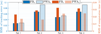
Figure 5: RMS of tracking errors and computation time of the two controllers with different types of references (distinguished, respectively, by the subscript $e$ and $t$ under the name of the corresponding controller).

In details, one shortcoming of FB-MPC is that it demands slightly more execution time than the PWA-MPC in practice. This can be explained by showing the complexity of the optimization problems. Particularly, both the PWA-MPC and FB-MPC as in (19) are quadratic programming problems. However, the constraint set $\mathcal{S}_{v}$ is computationally complex, compared to $\mathcal{U}$ with more vertices or inequalities. The effect can also be seen in Fig. 5 with a roughly constant gap in computation time necessary for the two methods.

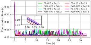
Figure 6: Computation time used for different references.

Yet, since PWA-MPC depends on the approximation of the model along the trajectory, its efficiency is reliant on the reference’s quality, hence making the method more vulnerable to uncertainty than our proposed FB-MPC. Indeed, while with Ref. 1, both controllers achieve fairly good tracking (See Fig. 5), with Ref. 2, large oscillations in tracking error are observed with PWA-MPC compared to that of the FB-MPC (see Fig. 7). Moreover, despite being constructed via an approximated input constraint, the FB-MPC always shows an equivalently reliable performance without saturating the input, in comparison with the PWA-MPC, as in Fig. 8.

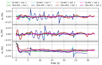
Figure 7: Crazyflie tracking error with flatness-based MPC and PWA-MPC (4 references) with $e_{q}\triangleq q^{\mathrm{ref}}-q,\;q\in\{x,y,z\}$.

Furthermore, due to the fact that there is no approximation in our model, the performance in the proposed FB-MPC surpasses its approximation-based contestant in [17] with Ref. 3. Finally, although being constructed in the similar framework of flatness-based MPC, with Ref. 4, our improved performance is apparent thanks to the less conservative constraint set $\mathcal{S}_{v}$ as opposed to the box-type set in [6].

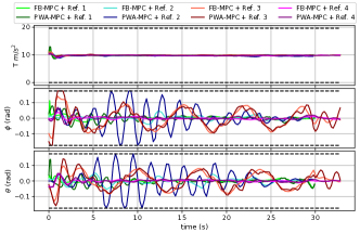
Figure 8: Input signals with their constraints (black dashed line).

V Conclusion

This paper presented a reliable FB-MPC design for the quadcopter system by introducing an efficient approximation for the feasible domain in the flat output space, where the system is linearized in closed-loop. The validation demonstrates the advantages of the contributions compared to related works conducted in the literature. As future work, we attempt to adapt the procedure to other classes of flat systems, where the constraints are more geometrically distorted by the flatness-based coordinate change.

We adapt the implementation of PWA-MPC from [5] as follows. Along the system’s refernce trajectory, we choose $N_{l}$ points around which the dynamics is approximated by using Taylor expansion as:

$$\boldsymbol{\xi}_{k+1}=\boldsymbol{A}_{j}\boldsymbol{\xi}_{k}+\boldsymbol{B}_{j}\boldsymbol{u}_{k}+\boldsymbol{r}_{j}$$ (20)

with $\boldsymbol{f}_{d}$ in (18), $\boldsymbol{A}_{j}=\left.{\partial\boldsymbol{f}_{d}}/{\partial\boldsymbol{\xi}}\right|_{\boldsymbol{\xi}_{j},\boldsymbol{u}_{j}}$, $\boldsymbol{B}_{j}=\left.{\partial\boldsymbol{f}_{d}}/{\partial\boldsymbol{\xi}}\right|_{\boldsymbol{\xi}_{j},\boldsymbol{u}_{j}}$ and $\boldsymbol{r}_{j}=\boldsymbol{f}_{d}(\boldsymbol{\xi}_{j},\boldsymbol{u}_{j})-\boldsymbol{A}_{j}\boldsymbol{\xi}_{j}-\boldsymbol{B}_{j}\boldsymbol{u}_{j}$ while $\boldsymbol{\xi}_{j},\boldsymbol{u}_{j}$ respectively denote the $j$-th state and input value in the collection of $N_{l}$ points equidistantly chronologically sampled from the nominal trajectory. During the implementation, $\boldsymbol{A}_{j},\boldsymbol{B}_{j}$ and $\boldsymbol{R}_{j}$ are flexibly chosen according to the drone’s closest point. Hence, the online optimization problem is expressed as:

$$\underset{\mathclap{\boldsymbol{u}_{k},...,\boldsymbol{u}_{k\text{+}N_{p}-1}}}{\arg\min\;\;\;\;\;\,}\sum_{i=0}^{N_{p}-1}\|\boldsymbol{\xi}_{i+k}-\boldsymbol{\xi}_{i+k}^{\mathrm{ref}}\|_{\boldsymbol{Q}}^{2}+\|\boldsymbol{u}_{i+k}-\boldsymbol{u}_{i+k}^{\mathrm{ref}}\|_{\boldsymbol{R}}^{2}$$ (21)

$$\text{s.t :}\begin{cases}\boldsymbol{x}_{i+k+1}=\boldsymbol{A}_{j}\boldsymbol{\xi}_{i+k}+\boldsymbol{B}_{j}\boldsymbol{u}_{i+k}+\boldsymbol{r}_{j}\\ \boldsymbol{u}_{i+k}\in{\mathcal{U}},\,i\in\{0,1,...,N_{p}-1\}\end{cases}\vspace{-0.2cm}$$

with $\boldsymbol{\xi}_{k}^{\mathrm{ref}},\boldsymbol{v}_{k}^{\mathrm{ref}}$ denoting the reference for $\boldsymbol{\xi}_{k}$ and $\boldsymbol{u}_{k}$.

References

- [1] S. Formentin and M. Lovera, “Flatness-based control of a quadrotor helicopter via feedforward linearization,” in 2011 50th IEEE Conference on Decision and Control and European Control Conference. IEEE, 2011, pp. 6171–6176.
- [2] A. Freddi, A. Lanzon, and S. Longhi, “A feedback linearization approach to fault tolerance in quadrotor vehicles,” IFAC proceedings volumes, vol. 44, no. 1, pp. 5413–5418, 2011.
- [3] N. T. Nguyen, I. Prodan, and L. Lefèvre, “Stability guarantees for translational thrust-propelled vehicles dynamics through NMPC designs,” IEEE Transactions on Control Systems Technology, vol. 29, no. 1, pp. 207–219, 2020.
- [4] M. Fliess, J. Lévine, P. Martin, and P. Rouchon, “Flatness and defect of non-linear systems: introductory theory and examples,” International journal of control, vol. 61, no. 6, pp. 1327–1361, 1995.
- [5] I. Prodan, S. Olaru, F. A. Fontes, F. Lobo Pereira, J. Borges de Sousa, C. Stoica Maniu, and S.-I. Niculescu, “Predictive control for path-following. from trajectory generation to the parametrization of the discrete tracking sequences,” in Developments in Model-Based Optimization and Control. Springer, 2015, pp. 161–181.
- [6] M. Greeff and A. P. Schoellig, “Flatness-based model predictive control for quadrotor trajectory tracking,” in 2018 IEEE/RSJ International Conference on Intelligent Robots and Systems (IROS). IEEE, 2018.
- [7] M. W. Mueller and R. D’Andrea, “A model predictive controller for quadrocopter state interception,” in 2013 European Control Conference (ECC). IEEE, 2013, pp. 1383–1389.
- [8] D. Ioan, S. Olaru, S.-I. Niculescu, I. Prodan, and F. Stoican, “Navigation in a multi-obstacle environment. from partition of the space to a zonotopic-based MPC,” in 2019 18th European Control Conference (ECC). IEEE, 2019, pp. 1772–1777.
- [9] N. T. Nguyen, I. Prodan, and L. Lefèvre, “Effective angular constrained trajectory generation for thrust-propelled vehicles,” in 2018 European Control Conference (ECC). IEEE, 2018, pp. 1833–1838.
- [10] S. Boyd, S. P. Boyd, and L. Vandenberghe, Convex optimization. Cambridge university press, 2004.
- [11] P. McMullen, “On zonotopes,” Transactions of the American Mathematical Society, vol. 159, pp. 91–109, 1971.
- [12] D. Q. Mayne, S. V. Raković, R. Findeisen, and F. Allgöwer, “Robust output feedback model predictive control of constrained linear systems,” Automatica, vol. 42, no. 7, pp. 1217–1222, 2006.
- [13] F. Blanchini, S. Miani, and F. A. Pellegrino, “Suboptimal receding horizon control for continuous-time systems,” IEEE transactions on automatic control, vol. 48, no. 6, pp. 1081–1086, 2003.
- [14] I. Zafeiratou, I. Prodan, L. Lefèvre, and L. Piétrac, “Meshed DC microgrid hierarchical control: A differential flatness approach,” Electric Power Systems Research, vol. 180, p. 106133, 2020.
- [15] H. T. Do, I. Prodan, and F. Stoican, “Analysis of alternative flat representations of a UAV for trajectory generation and tracking,” in 2021 25th International Conference on System Theory, Control and Computing (ICSTCC). IEEE, 2021, pp. 58–63.
- [16] I. Prodan, F. Stoican, and C. Louembet, “Necessary and sufficient LMI conditions for constraints satisfaction within a b-spline framework,” in 2019 IEEE 58th Conference on Decision and Control. IEEE, 2019.
- [17] G. A. Garcia, A. R. Kim, E. Jackson, S. S. Keshmiri, and D. Shukla, “Modeling and flight control of a commercial nano quadrotor,” in 2017 International Conference on Unmanned Aircraft Systems (ICUAS). IEEE, 2017, pp. 524–532.