Reconfigurable Intelligent Surface-aided Secret Key Generation in Multi-Cell Systems

Abstract

Physical-layer key generation (PKG) exploits the reciprocity and randomness of wireless channels to generate a symmetric key between two legitimate communication ends. However, in multi-cell systems, PKG suffers from severe pilot contamination due to the reuse of pilots in different cells. In this paper, we invoke multiple reconfigurable intelligent surfaces (RISs) for adaptively shaping the environment and enhancing the PKG performance. To this end, we formulate an optimization problem to maximize the weighted sum key rate (WSKR) by jointly optimizing the precoding matrices at the base stations (BSs) and the phase shifts at the RISs. For addressing the non-convexity of the problem, we derive an upper bound of the WSKR and prove its tightness. To tackle the upper bound maximization problem, we apply an alternating optimization (AO)-based algorithm to divide the joint optimization into two sub-problems. We apply the Lagrangian dual approach based on the Karush-Kuhn-Tucker (KKT) conditions for the sub-problem of precoding matrices and adopt a projected gradient ascent (PGA) algorithm for the sub-problem of phase shifts. Simulation results confirm the near-optimal performance of the proposed algorithm and the effectiveness of RISs for improving the WSKR via mitigating pilot contamination.

I Introduction

The ever-increasing connectivity among a large number of devices and the ubiquitous wireless communications have aroused great awareness to establish secure communication on the fly [1]. Conventionally, secure communication is guaranteed by applying cryptographic encryption mechanisms in the application layer [2]. Particularly, symmetric keys should be distributed to legitimate parties in these mechanisms before the actual communication takes place. However, existing cryptographic techniques face difficulties to realize secret key sharing in ad-hoc and mobile networks [3]. As an alternative, physical-layer key generation (PKG) exploits the intrinsic reciprocity and randomness of wireless channels to generate a pair of secret keys between the desired legitimate ends [4]. Furthermore, due to the existence of spatial decorrelation, an eavesdropper, Eve, cannot obtain any information about the generated keys if she locates more than half a wavelength away from the legitimate ends, i.e., Alice and Bob [5, 6, 7].

The process of PKG generally consists of four steps: channel sounding, quantization, information reconciliation, and privacy amplification [7]. During the channel probing step, Alice and Bob exchange pilots to acquire highly correlated channel estimations. Then, the extracted channel estimations are respectively quantized into bit sequences at Alice and Bob in the quantization step. Also, during the information reconciliation step, error-correcting codes are adopted to correct the mismatched bits between Alice and Bob. Finally, privacy amplification is employed to erase the bits that might have leaked information to Eve in the previous probing and reconciliation steps. From the above steps, it can be seen that PKG highly relies on the inherent randomness and reciprocity of wireless channels. However, the desired secret key rate may not be guaranteed in some harsh propagation environments, such as wave-blockage environments [8], [9]. Fortunately, reconfigurable intelligent surface (RIS), which has emerged as a disruptive wireless communication technology, has great potential to address this problem. In fact, RIS is a planar surface comprising a large number of low-cost passive reflecting elements [10, 11, 12]. These elements can independently adjust the phase shifts to collaboratively customize the wireless propagation environment [12]. Therefore, it is expected that deploying RIS in secure communication can facilitate the required PKG. In particular, when the direct link between Alice and Bob is blocked, RIS could shape a RIS-induced fluctuating channel to serve as a controllable randomizer for generating a secret key.

However, to fully unleash the potential of the RIS for improving PKG performance, the optimization of the phase shifts of RIS is required. To date, several studies have focused on the design of phase shifts of RIS [13, 14, 9, 15, 16, 17]. For instance, [13, 14, 9] studied the reflection coefficients optimization in single-input single-output (SISO) systems with only one legitimate user. In particular, the authors in [13] assumed the RIS-induced channel of the eavesdropper is independent from that of the legitimate ends. Based on this, they derived the expression of the key generation rate (KGR) capacity and optimized the on/off states of the RIS units. Furthermore, in [14], the authors considered RIS-assisted PKG with multiple non-colluding eavesdroppers. They designed a semidefinite relaxation (SDR) and successive convex approximation (SCA)-based algorithm to maximize the secret key capacity lower bound. Then, a RIS-assisted multiuser key generation scheme was studied in [9], where the RIS configuration was optimized to maximize the sum secret key rate of multiple users. On the other hand, [15, 16, 17] investigated the beamforming optimization in multiple-input single-output (MISO) systems. In particular, [15] proposed a low-complexity block successive upper-bound minimization (BSUM) with the mirror-prox method to optimize the reflective beamforming at the RIS and the transmit beamforming at the base station (BS), with the consideration of the spatial correlation at both the BS and the RIS. In addition, [16] treated the coupled precoding matrix and phase-shift matrix as an equivalent variable and designed a water-filling algorithm to acquire its optimal solution. Then, they recovered the two matrices from the optimized variable. Furthermore, to obtain a computationally efficient suboptimal solution to the non-convex problem in [16], the authors in [17] adopted a machine learning-based algorithm to achieve a higher KGR.

Nevertheless, all of these works i.e., [13, 14, 9, 15, 16, 17], focus on the design of single-cell systems, while practical RIS-based PKG methods in multi-cell systems are still lacked. Indeed, in multi-cell systems, the same pilot pool is reused in different cells due to the limited time and frequency resources giving rise to the pilot contamination problem [18, 19, 20]. Over the last couple of years, considerable research efforts have been devoted for studying the impact of pilot contamination on spectral and energy efficiencies and the corresponding methods for alleviating the negative impacts caused by pilot interference [19, 20, 21, 22, 23]. However, all of these works aim for reducing the uplink channel estimation error that do not align the goal of PKG which aims for improving the reciprocity between channel estimations in the uplink and downlink. Indeed, pilot contamination exists in both the uplink and downlink channel probing phase in PKG systems that introduces non-reciprocal interference to the channel estimations at the BSs and the user terminals (UTs). Therefore, this channel asymmetry caused by multi-cell pilot contamination is expected to jeopardize the key generation performance. To tackle this problem, we propose to employ multiple RISs to assist the PKG in multi-cell networks. Specifically, by carefully altering the phase shifts introduced by multiple RISs, the inter-cell pilot interference reflected by the RISs and the interference in the direct channel can be harnessed such that they can be destructively superimposed at the desired communication nodes to minimize the interference power. Therefore, the proposed paradigm provides a new degrees of freedom (DoF) to facilitate multi-cell PKG in conjunction with the precoding matrices at the BSs. However, the BSs’ precoding matrices and the RISs’ phase shifts have to be jointly optimized to fully unleash the potential of RISs for effective KGR provisioning. More importantly, existing techniques in [13, 14, 9, 15, 16, 17] cannot be directly applied to multi-cell PKG systems since the inter-cell pilot contamination is not taken into consideration.

To address the above issues, this paper investigates the PKG method in multi-cell systems. We introduce RISs to combat multi-cell pilot contamination by jointly optimizing the precoding matrices at the BSs and the phase shifts at the RISs. More specifically, the main contributions of this paper are as follows.

• We propose a novel RIS-aided multi-cell PKG framework based on the precoding matrices at the BSs and the phase shifts at the RISs. We then derive a closed-form KGR expression that facilitates the formulation of an optimization problem to maximize the weighted sum key rate (WSKR) of all the cells. Since the formulated problem is non-convex and difficult to solve, we derive a tight upper bound of the WSKR and maximize the upper bound.

• To tackle the upper bound maximization problem, we employ an alternating optimization (AO)-based algorithm to alternately obtain a high-quality suboptimal solution. To be specific, a Lagrangian dual algorithm based on the KKT conditions is applied to design the precoding matrices at the BSs and a PGA algorithm is adopted to optimize the phase shifts at the RISs.

• Simulation results verify that the WSKR by the proposed algorithm approaches the upper bound, showing the near-optimal performance. Also, a significant WSKR improvement can be observed with the increase of RIS elements number. Finally, distributed RISs, with each RIS being located in the proximity of some UTs, offer rich spatial diversity to maximize the WSKR.

Notations: In this paper, $\mathbb{C}^{A\times B}$ denotes the space of complex matrices of size $A\times B$. Matrices and vectors are denoted by boldface capital and lower-case letters, respectively. The imaginary unit of a complex number is denoted by $j=\sqrt{-1}$. $(\cdot)^{T}$ and $(\cdot)^{H}$ denote transpose and conjugate transpose, respectively. ${\rm{diag}}({\mathbf{x}})$ denotes a diagonal matrix whose diagonal elements are extracted from vector ${\mathbf{x}}$. $\rm{vec}({\mathbf{X}})$ denotes the vectorization of matrix ${\mathbf{X}}$. ${\rm{tr}}(\cdot)$ represents the trace of a matrix. $\triangleq$ means “defined as”. $\otimes$ denotes the Kronecker product. $\mathcal{I}(X;Y)$ and $\mathcal{H}(X,Y)$ are the mutual information and joint entropy of random variables $X$ and $Y$, respectively. $\operatorname{det}(\cdot)$ is the matrix determinant. $\|{\mathbf{X}}\|_{F}$ is the Frobenius norm of matrix ${\mathbf{X}}$. $\mathbb{E}\{\cdot\}$ represents statistical expectation. $\lambda_{\ell}({\mathbf{X}})$ is the $\ell$-th largest eigenvalue of matrix ${\mathbf{X}}$. $\mathcal{O}(\cdot)$ is the big-O notation. $\left[{\mathbf{X}}\right]_{m:n,i}$ means the matrix consisting of rows $m$ to $n$ and column $i$ of matrix ${\mathbf{X}}$. $\nabla f(\cdot)$ and $\partial f/\partial x$ are the gradient operator of function $f$. ${\mathbf{I}}_{M}$ denotes the identity matrix of dimension $M$.

II RIS-based Multi-Cell Key Generation Model

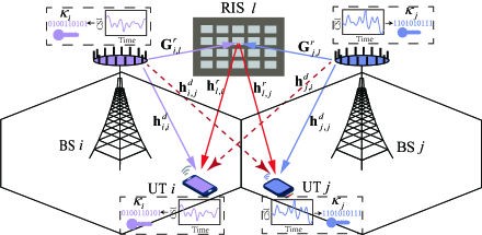
Figure 1: The model of RIS-aided PKG in multi-cell systems.

As shown in Fig. 1, we consider a multi-cell PKG model constituted by $K$ cells, each of which has an $M$ antennas BS and a single-antenna UT. Under the time-division duplexing (TDD) protocol, the BS and UT in the $k$-th cell, i.e., BS $k$ and UT $k$, $k\in\left\{1,\cdots,K\right\}$, aim to generate a symmetric key ${\kappa}_{k}$ by exploiting the reciprocity of the involved wireless channels. To facilitate the PKG, the system deploys $L$ RISs with each RIS consisting of $N$ passive reflection elements. Besides, there is a smart controller for coordinating the BSs and adapting the phase shifts of the RISs to enable effective secret key generation [25].

II-A RIS-based Channel Model

The direct channel between UT $j$ and BS $i$ is denoted as ${\mathbf{h}}_{i,j}^{d}\in\mathbb{C}^{M\times 1},i,j\in\{1,\cdots,K\}$. When the RISs are introduced to the PKG system, they establish some indirect additional communication channels. Specifically, the channels from BS $i$ to RIS $l$, $l\in\left\{1,\cdots,L\right\}$, and from RIS $l$ to UT $j$ are denoted as ${\mathbf{G}}_{i,l}^{r}\in\mathbb{C}^{M\times N}$ and ${\mathbf{h}}_{l,j}^{r}\in\mathbb{C}^{N\times 1}$, respectively. The diagonal phase-shifting matrix of RIS $l$ is denoted by $\hbox{\boldmath$\Phi$}_{l}={\rm{diag}}\{{\mathbf{v}}_{l}\}$, where ${\mathbf{v}}_{l}\in\mathbb{C}^{N\times 1}$ is the phase-shifting vector adopted at RIS $l$. Then, the equivalent downlink channel from BS $i$ to UT $j$ is expressed as

$${\mathbf{h}}_{i,j} ={\mathbf{h}}_{i,j}^{d}+\sum_{l=1}^{L}{\mathbf{G}}_{i,l}^{r}\hbox{\boldmath$\Phi$}_{l}{\mathbf{h}}_{l,j}^{r}={\mathbf{h}}_{i,j}^{d}+{\mathbf{H}}_{i,j}^{r}{\mathbf{v}},$$ (1)

where ${\mathbf{H}}_{i,j}^{r}={\mathbf{G}}_{i}^{r}{\rm{diag}}\{{\mathbf{h}}_{j}^{r}\}$ with ${\mathbf{G}}_{i,l}^{r}=\left[{\mathbf{G}}_{i,1}^{r},\cdots,{\mathbf{G}}_{i,L}^{r}\right]$ and ${\mathbf{h}}_{j}^{r}=\left[({\mathbf{h}}_{l,j}^{r})^{H},\cdots,({\mathbf{h}}_{l,j}^{r})^{H}\right]^{H}$. The phase-shifting vector at the RISs is ${\mathbf{v}}=\left[{\mathbf{v}}_{1}^{T},\cdots,{\mathbf{v}}_{L}^{T}\right]^{T}$.

From (1), the channel between BS $i$ and UT $j$ depends on the wireless channels and phase-shifting vector ${\mathbf{v}}$. This provides a new DoF for optimizing the key generation performance. Also, the multi-antenna BSs have the intrinsic capability of signal processing in the spatial domain. Hence, we next establish a new PKG framework to exploit the spatial diversity of the multi-antenna BSs and the environment-controlling characteristic of the RISs to enable the multi-cell secret key generation.

II-B RIS-aided PKG Framework

As shown in Fig. 2, the proposed framework consists of three phases. Firstly, during the parameter design phase, the BSs design the precoding matrices and phase-shifting vector. Then, they convey the phase-shifting vector to the RISs controller to configure the RISs reflection matrix. Secondly, the BSs and UTs acquire the channel estimations by channel probing. Finally, feature-to-key processing is performed to convert the channel estimations into secret keys [6], [9]. The specific procedures are shown as follows.

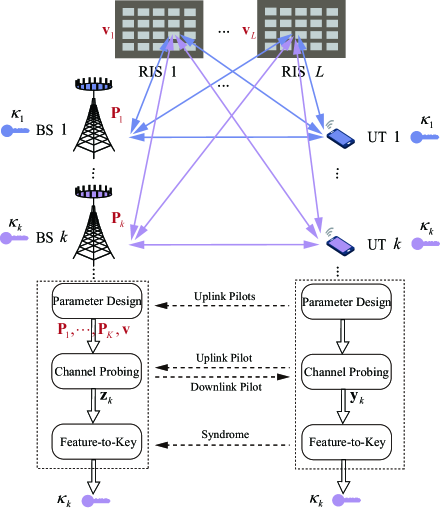
Figure 2: The proposed RIS-aided PKG framework in multi-cell systems.

1. Parameter Design: In this step, the BSs design the precoding matrices ${\mathbf{P}}_{k},k\in\left\{1,\cdots,K\right\}$, and phase shifts ${\mathbf{v}}$ according to some statistical CSI. In particular, the UTs in all the cells transmit orthogonal sounding signals such that the BSs can obtain the channel covariance matrices between the BSs and the UTs. Then, the BSs design the parameters ${\mathbf{P}}_{k}$ and ${\mathbf{v}}$ via the proposed optimization algorithm, which will be elaborated in Section IV.

2. Channel Probing: In this step, the BSs and UTs probe the channel alternatively and extract the reciprocal channel characteristics with the help of the precoding matrices and reflection coefficients. In the downlink, each BS transmits the downlink pilot signals processed by the optimized precoding matrix ${\mathbf{P}}_{k}$. Then, the UTs estimate the combined channels from the received signals. In the uplink, each UT transmits the same pilot signals. The pilot is reflected by the RISs and received by the BSs. Then, the BSs estimate the channels from the received signals and utilize the precoding matrices ${\mathbf{P}}_{k}$ to form the combined channels.

3. Feature-to-Key Processing: Once the BSs and UTs acquire the channel estimations, they employ some quantization method to generate raw key bits. Finally, information reconciliation and privacy amplification steps are performed to produce the secret keys.

Remark 1.

In the parameter design step, the prior information to design the precoding matrices and phase shifts are the channel covariance matrices. Due to the fact that the covariance matrices alter slowly across time in dense scattering environments [26], we can obtain these matrices from the previous several time slots by adopting some existing estimation methods e.g., [19], [21]. Upon the parameter design phase is completed, the BSs and UTs can perform multiple channel probing rounds within some channel coherence times. Each channel probing round is completed within one coherence time to guarantee the similarity of the uplink and downlink channel estimations. Meanwhile, different channel probing rounds should be performed in different coherence times to introduce randomness to the secret keys.

In this paper, we first focus on the channel probing step, where the multi-cell pilot contamination exists and then propose an algorithm to design the precoding matrices and phase shifts to improve the PKG performance.

II-C Signal Presentation of the Channel Probing

In the PKG system, the BSs and UTs first perform channel probing to acquire the reciprocal channel estimation. The process of channel probing is described as follows.

The channel sounding step contains two phases, i.e., the downlink phase and the uplink phase, respectively. In the downlink, BS $k$ transmits the downlink public known pilot ${\mathbf{X}}\in\mathbb{C}^{M_{e}\times M_{e}}$ with ${\mathbf{X}}{\mathbf{X}}^{H}={\mathbf{I}}_{M_{e}}$ and $M_{e}\leq M$ is the number of radio-frequency (RF) chains. Then, the signals received at UT $k$ is

$$\left({\mathbf{r}}_{k}^{d}\right)^{T}={\mathbf{h}}_{k,k}^{T}{\mathbf{P}}_{k}^{T}{\mathbf{X}}+\underbrace{\sum_{i=1,i\neq k}^{K}{\mathbf{h}}_{i,k}^{T}{\mathbf{P}}_{i}^{T}{\mathbf{X}}}_{\rm Signals\ from\ BSs\ in\ other\ cells}+({\mathbf{n}}_{k}^{d})^{T},$$ (2)

where ${\mathbf{P}}_{i}\in\mathbb{C}^{M_{e}\times M}$ represents the precoding matrix at BS $i$ [6], [27], ${\mathbf{n}}_{k}^{d}\in\mathbb{C}^{M_{e}\times 1}$ is the complex Gaussian noise at UT $k$ with zero mean and unit variance. After the standard least-squares (LS) channel estimation [9], [14], UT $k$ obtains

$${\mathbf{y}}_{k}={\mathbf{X}}^{*}{\mathbf{r}}_{k}^{d}={\mathbf{P}}_{k}{\mathbf{h}}_{k,k}+\sum_{i=1}^{K}{\mathbf{P}}_{i}{\mathbf{h}}_{i,k}+{\mathbf{X}}^{*}{{\mathbf{n}}}_{k}^{d}.$$ (3)

In the uplink phase, the UTs simultaneously transmits the pilot $s$ with $|s|^{2}=1$ and the signal received at BS $k$ is expressed as

$${\mathbf{r}}_{k}^{u}={\mathbf{h}}_{k,k}s+\underbrace{\sum_{j=1,j\neq k}^{K}{\mathbf{h}}_{k,j}s}_{\rm Signals\ from\ UTs\ in\ other\ cells}+{\mathbf{n}}^{u}_{k},$$ (4)

where ${\mathbf{n}}^{u}_{k}$ is the complex Gaussian noise zero mean and unit variance. Then, BS $k$ performs the LS channel estimation as

$$\tilde{{\mathbf{z}}}_{k}={\mathbf{h}}_{k,k}+\sum_{j=1,j\neq k}^{K}{\mathbf{h}}_{k,j}+s^{*}{{\mathbf{n}}}_{k}^{u}.$$ (5)

Then, BS $k$ multiplies the channel estimation with the precoding matrix ${\mathbf{P}}_{k}$ that yields

$${\mathbf{z}}_{k}={\mathbf{P}}_{k}\tilde{{\mathbf{z}}}_{k}={\mathbf{P}}_{k}{\mathbf{h}}_{k,k}+{\mathbf{P}}_{k}\sum_{j=1,j\neq k}^{K}{\mathbf{h}}_{k,j}+{\mathbf{P}}_{k}s^{*}{{\mathbf{n}}}_{k}^{u}.$$ (6)

It can be observed from (3) and (6) that the extracted channel features at BS $k$ and UT $k$ include the reciprocal component ${\mathbf{P}}_{k}{\mathbf{h}}_{k,k}$, the inter-cell interference, and as well as the noise component. These interference terms are not perfectly reciprocal. In particular, in the $k$-th cell, the interference in the uplink, i.e., ${\mathbf{P}}_{k}\sum_{j=1,j\neq k}{\mathbf{h}}_{k,j}$, is the product of ${\mathbf{P}}_{k}$ and the aggregated channels from UT $j$ to BS $k$, while in the downlink, the interference, i.e., $\sum_{i=1,i\neq k}{\mathbf{P}}_{i}{\mathbf{h}}_{i,k}$, is the superimposed channels from BS $i$ to UT $k$. Fortunately, these components are influenced by the precoding matrices ${\mathbf{P}}_{i},i\in\{1,\cdots,K\}$, at the BSs and the RIS phase-shifting vector ${\mathbf{v}}$. Next, we will analyze the impact of ${\mathbf{P}}_{i}$ and ${\mathbf{v}}$ on KGR.

III Secret Key Rate Analysis

In this section, based on the channel estimations shown in Section II, we derive the closed-form KGR expression and formulate an optimization problem with respect to (w.r.t.) the variables ${\mathbf{P}}_{i},i\in\{1,\cdots,K\}$, and ${\mathbf{v}}$. Then, to facilitate the design, we derive an upper bound of the KGR and formulate an upper bound maximization problem.

III-A KGR Analysis

To evaluate the key generation performance, we derive the KGR expression in the following. The KGR is a comprehensive metric to evaluate the consistency, rate, and randomness of the secret key [28]. The KGR between UT $k$ and BS $k$ is defined as the mutual information between their channel estimations, which is expressed as

$$R_{k}=\mathcal{I}({\mathbf{y}}_{k};{\mathbf{z}}_{k}).$$ (7)

Given the combined channel gains ${\mathbf{y}}_{k}$ and ${\mathbf{z}}_{k}$ in (3) and (6), the closed-form expression of the KGR can be derived as follows.

Theorem 1.

The KGR of UT $k$ and BS $k$ is given by

$$R_{k} =\ln\det\left({\mathbf{P}}_{k}\left[\sum_{j=1}^{K}{\mathbf{R}}_{k,j}^{d}+\left(\bar{{\mathbf{v}}}^{H}\otimes{\mathbf{I}}_{M}\right)\sum_{j=1}^{K}{\mathbf{R}}_{k,j}^{r}\left(\bar{{\mathbf{v}}}\otimes{\mathbf{I}}_{M}\right)+{\mathbf{I}}_{M}\right]{\mathbf{P}}_{k}^{H}\right)$$

$$\quad-\ln\det\left({\mathbf{P}}_{k}\left[\sum_{j=1}^{K}{\mathbf{R}}_{k,j}^{d}+\left(\bar{{\mathbf{v}}}^{H}\otimes{\mathbf{I}}_{M}\right)\sum_{j=1}^{K}{\mathbf{R}}_{k,j}^{r}\left(\bar{{\mathbf{v}}}\otimes{\mathbf{I}}_{M}\right)+{\mathbf{I}}_{M}\right]{\mathbf{P}}_{k}^{H}\right.$$

$$\quad\left.-{\mathbf{P}}_{k}\left({\mathbf{R}}_{k,k}^{d}+\left(\bar{{\mathbf{v}}}^{H}\otimes{\mathbf{I}}_{M}\right){\mathbf{R}}_{k,k}^{r}\left(\bar{{\mathbf{v}}}\otimes{\mathbf{I}}_{M}\right)\right){\mathbf{P}}_{k}^{H}\right.$$

$$\quad\left.\times\left(\sum_{i=1}^{K}{\mathbf{P}}_{i}\left({\mathbf{R}}_{i,k}^{d}+\left(\bar{{\mathbf{v}}}^{H}\otimes{\mathbf{I}}_{M}\right){\mathbf{R}}_{i,k}^{r}\left(\bar{{\mathbf{v}}}^{H}\otimes{\mathbf{I}}_{M}\right)^{H}\right){\mathbf{P}}_{i}^{H}+{\mathbf{I}}_{M_{e}}\right)^{-1}\right.$$

$$\quad\left.\times{\mathbf{P}}_{k}\left({\mathbf{R}}_{k,k}^{d}+\left(\bar{{\mathbf{v}}}^{H}\otimes{\mathbf{I}}_{M}\right){\mathbf{R}}_{k,k}^{r}\left(\bar{{\mathbf{v}}}\otimes{\mathbf{I}}_{M}\right)\right){\mathbf{P}}_{k}^{H}\right),$$ (8)

where ${\mathbf{R}}_{i,j}^{d}\stackrel{{\scriptstyle\Delta}}{{=}}\mathbb{E}\left\{{\mathbf{h}}_{i,j}^{d}\left({\mathbf{h}}_{i,j}^{d}\right)^{H}\right\}$ and ${\mathbf{R}}_{i,j}^{r}\stackrel{{\scriptstyle\Delta}}{{=}}\mathbb{E}\left\{{\rm vec}\left({\mathbf{H}}_{i,j}^{r}\right){\rm vec}\left({\mathbf{H}}_{i,j}^{r}\right)^{H}\right\}$ are the channel covariance of the direct channel and the RISs-involved channel between BS $i$ and UT $j$, respectively. The variable is defined as $\bar{{\mathbf{v}}}\stackrel{{\scriptstyle\Delta}}{{=}}{\mathbf{v}}^{*}$ for the sake of notational simplicity.

Proof.

Please see Appendix -A. ∎

Remark 2.

When the precoding matrices at the BSs are not optimized, i.e., ${\mathbf{P}}_{i}=\sqrt{\frac{P_{i}}{M}}{\mathbf{I}}_{M}$, and the RISs are not deployed, the KGR between BS $k$ and UT $k$ is given by

$$R_{k} =\ln\det\left(\sum_{j=1}^{K}{\mathbf{R}}^{d}_{k,j}+{\mathbf{I}}_{M}\right)-\ln\det\left(\sum_{j=1}^{K}{\mathbf{R}}^{d}_{k,j}+{\mathbf{I}}_{M}-{\frac{P_{k}}{M}}{\mathbf{R}}^{d}_{k,k}\left(\sum_{i=1}^{K}{\frac{P_{i}}{M}}{\mathbf{R}}^{d}_{i,k}+{\mathbf{I}}_{M}\right)^{-1}{\mathbf{R}}^{d}_{k,k}\right),$$ (9)

where $P_{i}$ denotes the transmit power at BS $i$. Furthermore, we present a proposition of the KGR performance as follows.

Proposition 1.

$R_{k}$ decreases monotonically with increasing $P_{i},i\neq k$, and the eigenvalues of ${\mathbf{R}}^{d}_{i,k}$ and ${\mathbf{R}}^{d}_{k,j},j\neq k$. Also, $R_{k}$ approaches $0$ when these values are sufficiently large.

Proof.

Please see Appendix -B. ∎

Proposition 1 proves that the KGR between BS $k$ and UT $k$ decreases with the transmit power of BSs in other cells, i.e., $P_{i},i\neq k$, and the channel gain of the interference channels, i.e., $\lambda_{\ell}\left({\mathbf{R}}^{d}_{i,k}\right),i\neq k$, and $\lambda_{\ell}\left({\mathbf{R}}^{d}_{k,j}\right),j\neq k$, $\ell\in\left\{1,\cdots,M\right\}$. In addition, $R_{k}$ tends to $0$ when these interference is sufficiently large. Therefore, the crux of the multi-cell PKG is to effectively mitigate the pilot contamination in the uplink and downlink.

Remark 3.

From (8), the KGR $R_{k}$ is decided by the statistical channel information (CSI), i.e., the channel covariance matrices, and the parameters, i.e., the precoding matrices and the phase-shifting vector. In this paper, we assume that the covariance matrices are perfectly known by the BSs in the parameter design phase and we focus on the design of precoding matrices and phase-shifting vector.

Now, we jointly design the precoding matrices and phase shifts to improve the key generation performance. Specifically, we aim for maximizing the WSKR of all the cells by jointly optimizing the ${\mathbf{P}}_{i},i\in\{1,\cdots,K\}$, and $\bar{{\mathbf{v}}}$, while guaranteeing the total power constraint of each BS and the unit modulus of the reflection coefficient of each RIS element. Specifically, the optimization problem can be formulated as

$$\underset{{\mathbf{P}}_{i},i\in\{1,\cdots,K\},{\bar{{\mathbf{v}}}}}{\text{maximize}}\ \sum_{k=1}^{K}w_{k}R_{k}$$

s.t. $$\ \text{C1}{:}\,||{\mathbf{P}}_{i}||_{F}^{2}\leq P_{\mathrm{A}},\forall i\in\{1,\cdots,K\},$$

$$\ \text{C2}{:}\,|v_{n}|\ =1,\forall n\in\{1,\cdots,NL\},$$ (10)

where $w_{k}\geq 0$ denotes the weight for the $k$-th cell that represents the priority of the corresponding BS and UT. Constraint C1 represents the power of the precoding matrices at each BS should be less than the maximum transmit power $P_{\rm A}$ [27]. Constraint C2 represents the modulus constraint of each reflection coefficient at the RISs [29].

Note that the objective function WSKR is non-convex w.r.t. ${\mathbf{P}}_{i}$ and $\bar{{\mathbf{v}}}$ since these variables are coupled in the matrix inversion operation. Additionally, the unit-modulus constraint C2 is also non-convex. Hence, Problem (10) is generally NP-hard and difficult to find the globally optimal solution [30]. Next, as a compromise, we derive an upper bound of the KGR and formulate an upper bound maximization problem.

III-B Upper Bound of KGR

Recalling (5) and (6), the channel estimation and the combined channel at BS $k$ are $\tilde{{\mathbf{z}}}_{k}=\sum_{j=1}^{K}{\mathbf{h}}_{k,j}+s^{*}{{\mathbf{n}}}_{k}^{u}$ and ${\mathbf{z}}_{k}={\mathbf{P}}_{k}\tilde{{\mathbf{z}}}_{k}$, respectively. Therefore, ${\mathbf{y}}_{k}$ and ${{\mathbf{z}}}_{k}$ are conditionally independent given $\tilde{{\mathbf{z}}}_{k}$, which means ${\mathbf{y}}_{k}$, $\tilde{{\mathbf{z}}}_{k}$, and ${\mathbf{z}}_{k}$ form a Markov chain ${\mathbf{y}}_{k}\rightarrow\tilde{{\mathbf{z}}}_{k}\rightarrow{\mathbf{z}}_{k}$. According to the data-procesing inequality [31], an upper bound of the KGR can be expressed as $R_{k}=\mathcal{I}({\mathbf{y}}_{k};{\mathbf{z}}_{k})\leq\mathcal{I}({\mathbf{y}}_{k};\tilde{{\mathbf{z}}}_{k})\stackrel{{\scriptstyle\Delta}}{{=}}R_{k}^{\rm ub}$. Then, the closed-form expression of $R_{k}^{\rm ub}$ can be derived as follows.

Theorem 2.

The KGR of $k$-th cell, $R_{k}$, is upper bounded by

$$R_{k}^{\rm ub}=\ln\det\left(\sum_{i=1}^{K}{\mathbf{P}}_{i}{\mathbf{M}}_{i,k}{\mathbf{P}}_{i}^{H}+{\mathbf{I}}_{M_{e}}\right)-\ln\det\left(\sum_{i=1}^{K}{\mathbf{P}}_{i}{\mathbf{M}}_{i,k}{\mathbf{P}}_{i}^{H}+{\mathbf{I}}_{M_{e}}-{\mathbf{P}}_{k}{\mathbf{N}}_{k,k}{\mathbf{P}}_{k}^{H}\right),$$ (11)

where

$${\mathbf{M}}_{i,k} ={\mathbf{R}}_{i,k}^{d}+\left(\bar{{\mathbf{v}}}^{H}\otimes{\mathbf{I}}_{M}\right){\mathbf{R}}_{i,k}^{r}\left(\bar{{\mathbf{v}}}^{H}\otimes{\mathbf{I}}_{M}\right)^{H},$$ (12)

$${\mathbf{N}}_{k,k} =\left({\mathbf{R}}_{k,k}^{d}+\left(\bar{{\mathbf{v}}}^{H}\otimes{\mathbf{I}}_{M}\right){\mathbf{R}}_{k,k}^{r}\left(\bar{{\mathbf{v}}}\otimes{\mathbf{I}}_{M}\right)\right){\mathbf{R}}_{\tilde{{\mathbf{z}}}_{k}}^{-1}\left({\mathbf{R}}_{k,k}^{d}+\left(\bar{{\mathbf{v}}}^{H}\otimes{\mathbf{I}}_{M}\right){\mathbf{R}}_{k,k}^{r}\left(\bar{{\mathbf{v}}}\otimes{\mathbf{I}}_{M}\right)\right).$$ (13)

Proof.

Please see Appendix -C. ∎

Remark 4.

We next prove the tightness of the derived upper bound. Specifically, the sufficient condition for achieving the upper bound, i.e., $R_{k}^{\rm ub}=R_{k}$, is $\mathcal{I}({\mathbf{y}}_{k};\tilde{{\mathbf{z}}}_{k}|{\mathbf{z}}_{k})=0$. In other words, ${\mathbf{y}}_{k}$, ${\mathbf{z}}_{k}$, and $\tilde{{\mathbf{z}}}_{k}$ also form a Markov chain ${\mathbf{y}}_{k}\rightarrow{\mathbf{z}}_{k}\rightarrow\tilde{{\mathbf{z}}}_{k}$ [31]. Therefore, one typical case for the equality hold is $M_{e}=M$ such that $\mathcal{I}({\mathbf{y}}_{k};\tilde{{\mathbf{z}}}_{k}|{\mathbf{P}}_{k}\tilde{{\mathbf{z}}}_{k})=\mathcal{H}(\tilde{{\mathbf{z}}}_{k}|{\mathbf{P}}_{k}\tilde{{\mathbf{z}}}_{k})-\mathcal{H}(\tilde{{\mathbf{z}}}_{k}|{\mathbf{y}}_{k},{\mathbf{P}}_{k}\tilde{{\mathbf{z}}}_{k})=0$. This means when the number of RF chains at the BS is the same as the number of antennas, the derived upper bound is tight and equal to the actual KGR.

Thanks to Theorem 2, the objective function is significantly simplified. Then, the upper bound optimization problem can be expressed as

$$\underset{{\mathbf{P}}_{i},i\in\{1,\cdots,K\},{\bar{{\mathbf{v}}}}}{\text{maximize}}\ \ \sum_{k=1}^{K}w_{k}R_{k}^{\rm ub}$$

s.t. $$\ \text{C1},\text{C2}.$$ (14)

It can be seen that the variables ${\mathbf{P}}_{i},i=1,\cdots,K$, and $\bar{{\mathbf{v}}}$ are still coupled in the objective function of Problem (14). In the next section, we apply an AO-based algorithm to alternately solve for $\left\{{\mathbf{P}}_{1},\cdots,{\mathbf{P}}_{K}\right\}$ and $\bar{{\mathbf{v}}}$ while fixing one of the variable sets.

IV AO-based Algorithm for Maximum Upper Bound

In this section, we provide an AO-based algorithm to tackle Problem (14). Specifically, to tackle the coupling of the optimization variables, we divide the joint problem into two sub-problems, each of which optimizes $\left\{{\mathbf{P}}_{1},\cdots,{\mathbf{P}}_{K}\right\}$ or $\bar{{\mathbf{v}}}$. For the sub-problem for $\left\{{\mathbf{P}}_{1},\cdots,{\mathbf{P}}_{K}\right\}$, we apply a Lagrangian multiplier method based on KKT conditions, while the sub-problem for $\bar{{\mathbf{v}}}$ is solved by the PGA algorithm.

IV-A Optimization of the Precoding Matrices at the BSs

We first present the optimization of precoding matrices $\left\{{\mathbf{P}}_{1},\cdots,{\mathbf{P}}_{K}\right\}$ for given $\bar{{\mathbf{v}}}$. By denoting ${\mathbf{P}}=\left[{\mathbf{P}}_{1},\cdots,{\mathbf{P}}_{K}\right]$, the sub-problem of ${\mathbf{P}}$ optimization is given by

$$\underset{{\mathbf{P}}}{\text{maximize}}\ \ \bar{g}\left({\mathbf{P}}\right)=\sum_{k=1}^{K}w_{k}\left(\ln\det\left({\mathbf{P}}{\mathbf{M}}_{k}{\mathbf{P}}^{H}+{\mathbf{I}}_{M_{e}}\right)-\ln\det\left({\mathbf{P}}{\mathbf{N}}_{k}{\mathbf{P}}^{H}+{\mathbf{I}}_{M_{e}}\right)\right)$$

s.t. $$\ \text{C1},$$ (15)

where ${\mathbf{M}}_{k}={\rm{diag}}\left({\mathbf{M}}_{1,k},\cdots,{\mathbf{M}}_{K,k}\right)$ and ${\mathbf{N}}_{k}={\rm{diag}}\left({\mathbf{M}}_{1,k},\cdots,{\mathbf{M}}_{k,k}-{\mathbf{N}}_{k,k},\cdots,{\mathbf{M}}_{K,k}\right)$.

Problem (15) is still non-convex since the objective function is in high-order w.r.t. ${\mathbf{P}}$. To derive an efficient suboptimal solution, we employ the Lagrangian multiplier method to address this problem. Specifically, by introducing the Lagrange multipliers $\lambda_{i},i=1,\cdots,K$, the Lagrangian function of Problem (15) is

$$\mathcal{L}\left({\mathbf{P}}_{i},\lambda_{i}\right)=\sum_{k=1}^{K}w_{k}\left(\ln\det\left({\mathbf{P}}{\mathbf{M}}_{k}{\mathbf{P}}^{H}+{\mathbf{I}}_{M_{e}}\right)-\ln\det\left({\mathbf{P}}{\mathbf{N}}_{k}{\mathbf{P}}^{H}+{\mathbf{I}}_{M_{e}}\right)\right)-{\rm{tr}}\left[{\mathbf{P}}{{\mathbf{\Lambda}}}{\mathbf{P}}^{H}\right]+P_{\rm A}\sum_{i=1}^{K}\lambda_{i},$$ (16)

where ${{\mathbf{\Lambda}}}={\rm{diag}}\left(\lambda_{1}{\mathbf{I}}_{M},\cdots,\lambda_{K}{\mathbf{I}}_{M}\right)$ and $\lambda_{i}\geq 0,i\in\left\{1,\cdots,K\right\}$ is associated with the power constraint in C1 at BS $i$. By analyzing the KKT condition, we can characterize the structure of the suboptimal solution to ${\mathbf{P}}$ in the following theorem.

Theorem 3.

The KKT condition for Problem (15) is given by

$$\rm{vec}\left({\mathbf{P}}\right) =\left({{\mathbf{\Lambda}}}^{T}\otimes{\mathbf{I}}_{M_{e}}+\sum_{k=1}^{K}w_{k}\left({\mathbf{N}}_{k}^{T}\otimes\left({\mathbf{I}}_{M_{e}}+{\mathbf{P}}{\mathbf{N}}_{k}{\mathbf{P}}^{H}\right)^{-1}\right)\right)^{-1}$$

$$\quad\times\sum_{k=1}^{K}w_{k}\left(\left({\mathbf{M}}_{k}^{T}\otimes\left({\mathbf{P}}{\mathbf{M}}_{k}{\mathbf{P}}^{H}+{\mathbf{I}}_{M_{e}}\right)^{-1}\right)\rm{vec}\left({\mathbf{P}}\right)\right).$$ (17)

Proof.

Please see Appendix -D. ∎

Next, the value of $\lambda_{i},i\in\left\{1,\cdots,K\right\}$, should be chosen for ensuring the power constraint at each BS in (14) is satisfied, which means

$$\lambda_{i}\left({\rm{tr}}({\mathbf{P}}_{i}{\mathbf{P}}_{i}^{H})-P_{\rm A}\right)=0.$$ (18)

To this end, recalling the KKT condition in (17), we can rewrite the $\text{vec}\left({\mathbf{P}}\right)$ as

$$\text{vec}\left({\mathbf{P}}\right) =\left({\rm{diag}}\left(\lambda_{1}{\mathbf{I}}_{MM_{e}},\cdots,\lambda_{K}{\mathbf{I}}_{MM_{e}}\right)+{\mathbf{F}}\right)^{-1}{\mathbf{a}}$$ (19)

$$={\rm{diag}}\left(\left(\lambda_{1}{\mathbf{I}}_{MM_{e}}+{\mathbf{F}}_{1}\right)^{-1},\cdots,\left(\lambda_{K}{\mathbf{I}}_{MM_{e}}+{\mathbf{F}}_{K}\right)^{-1}\right){\mathbf{a}},$$ (20)

where

$${\mathbf{F}}=\sum_{k=1}^{K}w_{k}\left({\mathbf{N}}_{k}^{T}\otimes\left({\mathbf{I}}_{M_{e}}+{\mathbf{P}}{\mathbf{N}}_{k}{\mathbf{P}}^{H}\right)^{-1}\right)={\rm{diag}}\left({\mathbf{F}}_{1},\cdots,{\mathbf{F}}_{K}\right),$$ (21)

and ${\mathbf{a}}=\sum_{k=1}^{K}w_{k}\left(\left({\mathbf{M}}_{k}^{T}\otimes\left({\mathbf{P}}{\mathbf{M}}_{k}{\mathbf{P}}^{H}+{\mathbf{I}}_{M_{e}}\right)^{-1}\right)\rm{vec}\left({\mathbf{P}}\right)\right)=\left[{\mathbf{a}}_{1}^{T},\cdots,{\mathbf{a}}_{K}^{T}\right]^{T}$. Thus, we can express the ${\mathbf{P}}_{i}$ at BS $i$ as

$$\text{vec}\left({\mathbf{P}}_{i}\right)=\left(\lambda_{1}{\mathbf{I}}_{MM_{e}}+{\mathbf{F}}_{i}\right)^{-1}{\mathbf{a}}_{i}.$$ (22)

By performing eigenvalue decomposition on matrix ${\mathbf{F}}_{i}$ as ${\mathbf{F}}_{i}={\mathbf{D}}_{i}{\rm{diag}}\left({\mathbf{f}}_{i}\right){\mathbf{D}}_{i}^{H}$, we have

$$\phi_{i}(\lambda_{i}) =\text{vec}\left({\mathbf{P}}_{i}\right)^{H}\text{vec}\left({\mathbf{P}}_{i}\right)$$ (23)

$$={\mathbf{a}}_{i}^{H}{\mathbf{D}}_{i}\left(\lambda_{i}{\mathbf{I}}_{MM_{e}}+{\rm{diag}}\left({\mathbf{f}}_{i}\right)\right)^{-1}\left(\lambda_{i}{\mathbf{I}}_{MM_{e}}+{\rm{diag}}\left({\mathbf{f}}_{i}\right)\right)^{-1}{\mathbf{D}}_{i}^{H}{\mathbf{a}}_{i}=\sum_{m=1}^{MM_{e}}\frac{b_{i,m}^{2}}{\left(\lambda_{i}+f_{i,m}\right)^{2}},$$ (24)

where ${\mathbf{f}}_{i}=[f_{i,1},\cdots,f_{i,MM_{e}}]^{T}$ and ${\mathbf{D}}_{i}^{H}{\mathbf{a}}_{i}=[b_{i,1},\cdots,b_{i,MM_{e}}]^{T}$. Since $f_{i,m}\geq 0$, it can be verified that $f_{i}(\lambda_{i})$ is a monotonically decreasing function w.r.t. $\lambda_{i}$.

Therefore, if $\phi_{i}(0)\leq P_{\rm A}$, the optimized ${\mathbf{P}}_{i}$ is $\text{vec}\left({\mathbf{P}}_{i}^{\rm KKT}\right)={\mathbf{F}}_{i}^{-1}{\mathbf{a}}_{i}$ when $\lambda_{i}$ is set to 0. On the other hand, if $\phi_{i}\left(0\right)>P_{\rm A}$, there exists a $\bar{\lambda}_{i}$ that satifies $\phi_{i}\left(\bar{\lambda}_{i}\right)=P_{\rm A}$. To find $\bar{\lambda}_{i}$, we can apply the bisection based search method and the upper bound of $\lambda_{i}$ is set as

$$\lambda_{i}^{\rm ub}=\sqrt{\frac{\sum_{m=1}^{M}b_{i,m}^{2}}{P_{\rm A}}},$$ (25)

since

$$\phi_{i}(\lambda_{i})<\sum_{m=1}^{M}\frac{b_{i,m}^{2}}{\left(\lambda_{i}^{\rm ub}\right)^{2}}=P_{\rm A}.$$ (26)

The overall algorithm to optimize ${\mathbf{P}}$ and $\lambda_{i},i\in\left\{1,\cdots,K\right\}$, is summarized as Algorithm 1.

Algorithm 1 The Lagrangian Dual Algorithm for Problem (15).

1:$w_{k},{\mathbf{M}}_{k}$, ${\mathbf{N}}_{k},k=1,\cdots,K$, $P_{\rm A},\epsilon$.

2:Set: $t=0$ (iteration index).

3:Initial: ${\mathbf{P}}^{(0)}$.

4:repeat

5:     Calculate ${{\mathbf{P}}}^{(t+1)}$ as

$${\rm vec}\left({\mathbf{P}}^{(t+1)}\right) =\left({{\mathbf{\Lambda}}}^{T}\otimes{\mathbf{I}}_{M_{e}}+\sum_{k=1}^{K}w_{k}\left({\mathbf{N}}_{k}^{T}\otimes\left({\mathbf{I}}_{M_{e}}+{\mathbf{P}}^{(t)}{\mathbf{N}}_{k}\left({\mathbf{P}}^{(t)}\right)^{H}\right)^{-1}\right)\right)^{-1}$$

$$\quad\times\sum_{k=1}^{K}w_{k}\left(\left({\mathbf{M}}_{k}^{T}\otimes\left({\mathbf{P}}^{(t)}{\mathbf{M}}_{k}\left({\mathbf{P}}^{(t)}\right)^{H}+{\mathbf{I}}_{M_{e}}\right)^{-1}\right){\rm vec}\left({\mathbf{P}}^{(t)}\right)\right).$$ (27)

6:     Set: $i=1$ (BS index).

7:     repeat

8:         Initialize the bounds $\lambda_{i}^{\rm ub}$ and $\lambda_{i}^{\rm lb}$.

9:         repeat

10:              If $\phi_{i}(0)\leq P_{A}$ holds, $\rm{vec}\left({\mathbf{P}}_{i}^{\text{KKT}}\right)={\mathbf{F}}_{i}^{-1}{\mathbf{a}}_{i}$; otherwise, go to the next step.

11:              Calculate $\lambda_{i}=\left(\lambda_{i}^{\rm ub}+\lambda_{i}^{\rm lb}\right)/2$.

12:              If $\phi_{i}(\lambda_{i})\leq P_{A}$, set $\lambda_{i}^{\rm ub}=\lambda_{i}$; Otherwise, set $\lambda_{i}^{\rm lb}=\lambda_{i}$.

13:         until $|\lambda_{i}^{\rm ub}-\lambda_{i}^{\rm lb}|\leq\epsilon$.

14:     until $i=K$.

15:     Set $t=t+1$ and calculate the secret key rate $\bar{g}({\mathbf{P}}^{(t+1)})$.

16:until $\frac{|\bar{g}({\mathbf{P}}^{(t+1)})-\bar{g}({\mathbf{P}}^{(t)})|}{\bar{g}({\mathbf{P}}^{(t)})}\leq\epsilon.$

IV-B Optimization of Phase Shifts at the RISs

Next, we present the optimization of phase shift vector $\bar{{\mathbf{v}}}$ when $\left\{{\mathbf{P}}_{1},\cdots,{\mathbf{P}}_{K}\right\}$ are fixed. To facilitate the algorithm design, we can first formulate the sub-problem for the RISs as

$$\underset{{\bar{{\mathbf{v}}}}}{\text{maximize}}\ \ \tilde{g}(\bar{{\mathbf{v}}})=\sum_{k=1}^{K}w_{k}R_{k}^{\rm ub}(\bar{{\mathbf{v}}})$$

s.t. $$\ \text{C2},$$ (28)

where

$$R_{k}^{\rm ub}(\bar{{\mathbf{v}}}) =\ln\det\left(\L_{k}\right)-\ln\det\left(\L_{k}-\left({\mathbf{P}}_{k}{\mathbf{R}}_{k,k}^{d}+{\left(\bar{{\mathbf{v}}}^{H}\otimes{\mathbf{I}}_{M_{e}}\right)}\left({\mathbf{I}}_{NL}\otimes{\mathbf{P}}_{k}\right){\mathbf{R}}_{k,k}^{r}{\left(\bar{{\mathbf{v}}}^{H}\otimes{\mathbf{I}}_{M}\right)^{H}}\right)\right.$$

$$\left.\quad\times\left(\sum_{j=1}^{K}{\mathbf{R}}_{k,j}^{d}+{\left(\bar{{\mathbf{v}}}^{H}\otimes{\mathbf{I}}_{M}\right)}\sum_{j=1}^{K}{\mathbf{R}}_{k,j}^{r}{\left(\bar{{\mathbf{v}}}^{H}\otimes{\mathbf{I}}_{M}\right)^{H}}+{\mathbf{I}}_{M}\right)^{-1}\right.$$

$$\left.\quad\times\left({\mathbf{R}}_{k,k}^{d}{\mathbf{P}}_{k}^{H}+{\left(\bar{{\mathbf{v}}}^{H}\otimes{\mathbf{I}}_{M}\right)}{\mathbf{R}}_{k,k}^{r}\left({\mathbf{I}}_{NL}\otimes{\mathbf{P}}_{k}\right)^{H}{\left(\bar{{\mathbf{v}}}^{H}\otimes{\mathbf{I}}_{M_{e}}\right)^{H}}\right)\right),$$ (29)

where $\L_{k}=\sum_{i=1}^{K}{\mathbf{P}}_{i}{\mathbf{R}}_{i,k}^{d}{\mathbf{P}}_{i}^{H}+{\left(\bar{{\mathbf{v}}}^{H}\otimes{\mathbf{I}}_{M_{e}}\right)}\sum_{i=1}^{K}\left({\mathbf{I}}_{NL}\otimes{\mathbf{P}}_{i}\right){\mathbf{R}}_{i,k}^{r}\left({\mathbf{I}}_{NL}\otimes{\mathbf{P}}_{i}\right)^{H}{\left(\bar{{\mathbf{v}}}^{H}\otimes{\mathbf{I}}_{M_{e}}\right)^{H}}+{\mathbf{I}}_{M_{e}}$. From (29), the objective function is intractable w.r.t. $\bar{{\mathbf{v}}}$. The unit modulus constraint C2 is also non-convex and there is no general approach to solve unit modulus constrained problems optimally. Therefore, we adopt the PGA algorithm to find a stationary solution of Problem (28) [32]. At each iteration, PGA projects the solution onto the closest feasible point satisfying the unit-modulus constraint.

Specifically, at iteration $t$, we first calculate the conjugate gradient $\nabla_{\bar{{\mathbf{v}}}^{*}}g(\bar{{\mathbf{v}}})$ as the ascent direction to guarantee the increase of the objective function. The closed-form expression of the gradient is derived as follows.

Theorem 4.

The Euclidean gradient of function $g(\bar{{\mathbf{v}}})$ w.r.t. $\bar{{\mathbf{v}}}^{*}$ is given by

$$\nabla_{\bar{{\mathbf{v}}}^{*}}g(\bar{{\mathbf{v}}})=\sum_{k=1}^{K}w_{k}\left(\sum_{m=1}^{M_{e}}\bar{{\mathbf{q}}}_{k,m}+\sum_{m=1}^{M}\bar{{\mathbf{g}}}_{k,m}\right),$$ (30)

where $\bar{{\mathbf{q}}}_{k,m}=\left[{\mathbf{Q}}_{k}\right]_{(m-1)NL+1:mNL,m}$, $\bar{{\mathbf{g}}}_{k,m}=\left[{\mathbf{G}}_{k}\right]_{(m-1)NL+1:mNL,m}$ and

$${\mathbf{Q}}_{k} ={\mathbf{K}}_{M_{e}NL}\sum_{i=1}^{K}\left({\mathbf{I}}_{NL}\otimes{\mathbf{P}}_{i}\right){\mathbf{R}}_{i,k}^{r}\left({\mathbf{I}}_{NL}\otimes{\mathbf{P}}_{i}\right)^{H}\left(\bar{{\mathbf{v}}}\otimes{\mathbf{I}}_{M_{e}}\right){\mathbf{R}}_{{\mathbf{y}}_{k}}^{-1}{\mathbf{K}}_{M_{e}}$$

$$\quad-{\mathbf{K}}_{M_{e}NL}\sum_{i=1}^{K}\left({\mathbf{I}}_{NL}\otimes{\mathbf{P}}_{i}\right){\mathbf{R}}_{i,k}^{r}\left({\mathbf{I}}_{NL}\otimes{\mathbf{P}}_{i}\right)^{H}\left(\bar{{\mathbf{v}}}\otimes{\mathbf{I}}_{M_{e}}\right)\left({\mathbf{R}}_{{\mathbf{y}}_{k}}-{\mathbf{R}}_{{\mathbf{y}}_{k}\tilde{{\mathbf{z}}}_{k}}{\mathbf{R}}_{\tilde{{\mathbf{z}}}_{k}}^{-1}{\mathbf{R}}_{\tilde{{\mathbf{z}}}_{k}{\mathbf{y}}_{k}}\right)^{-1}{\mathbf{K}}_{M_{e}}$$

$$\quad+{\mathbf{K}}_{M_{e}NL}\left({\mathbf{I}}_{NL}\otimes{\mathbf{P}}_{k}\right){\mathbf{R}}_{k,k}^{r}\left(\bar{{\mathbf{v}}}\otimes{\mathbf{I}}_{M}\right){\mathbf{R}}_{\tilde{{\mathbf{z}}}_{k}}^{-1}{\mathbf{R}}_{\tilde{{\mathbf{z}}}_{k}{\mathbf{y}}_{k}}\left({\mathbf{R}}_{{\mathbf{y}}_{k}}-{\mathbf{R}}_{{\mathbf{y}}_{k}\tilde{{\mathbf{z}}}_{k}}{\mathbf{R}}_{\tilde{{\mathbf{z}}}_{k}}^{-1}{\mathbf{R}}_{\tilde{{\mathbf{z}}}_{k}{\mathbf{y}}_{k}}\right)^{-1}{\mathbf{K}}_{M_{e}},$$

$${\mathbf{G}}_{k} =-{\mathbf{K}}_{MNL}\sum_{j=1}^{K}{\mathbf{R}}_{k,j}^{r}\left(\bar{{\mathbf{v}}}\otimes{\mathbf{I}}_{M}\right){\mathbf{R}}_{\tilde{{\mathbf{z}}}_{k}}^{-1}{\mathbf{R}}_{\tilde{{\mathbf{z}}}_{k}{\mathbf{y}}_{k}}\left({\mathbf{R}}_{{\mathbf{y}}_{k}}-{\mathbf{R}}_{{\mathbf{y}}_{k}\tilde{{\mathbf{z}}}_{k}}{\mathbf{R}}_{\tilde{{\mathbf{z}}}_{k}}^{-1}{\mathbf{R}}_{\tilde{{\mathbf{z}}}_{k}{\mathbf{y}}_{k}}\right)^{-1}{\mathbf{R}}_{{\mathbf{y}}_{k}\tilde{{\mathbf{z}}}_{k}}{\mathbf{R}}_{\tilde{{\mathbf{z}}}_{k}}^{-1}{\mathbf{K}}_{M}$$

$$\quad+{\mathbf{K}}_{MNL}{\mathbf{R}}_{k,k}^{r}\left({\mathbf{I}}_{NL}\otimes{\mathbf{P}}_{k}\right)^{H}\left(\bar{{\mathbf{v}}}\otimes{\mathbf{I}}_{M_{e}}\right)\left({\mathbf{R}}_{{\mathbf{y}}_{k}}-{\mathbf{R}}_{{\mathbf{y}}_{k}\tilde{{\mathbf{z}}}_{k}}{\mathbf{R}}_{\tilde{{\mathbf{z}}}_{k}}^{-1}{\mathbf{R}}_{\tilde{{\mathbf{z}}}_{k}{\mathbf{y}}_{k}}\right)^{-1}{\mathbf{R}}_{{\mathbf{y}}_{k}\tilde{{\mathbf{z}}}_{k}}{\mathbf{R}}_{\tilde{{\mathbf{z}}}_{k}}^{-1}{\mathbf{K}}_{M},$$ (31)

where ${\mathbf{K}}_{I}\in\mathbb{C}^{I\times I},I\in\left\{M_{e},M_{e}NL,MNL,M\right\}$, is the commutation matrix [33].

Proof.

Please see Appendix -E. ∎

Then, the next iteration point is calculated as $\bar{{\mathbf{v}}}^{(t+1)}=\exp\left(j\arg\left(\bar{{\mathbf{v}}}^{(t)}+\mu\nabla_{\bar{{\mathbf{v}}}^{*}}g(\bar{{\mathbf{v}}})\right)\right)$, where $\mu$ is the step size computed by the backtracking line search [30] and the $\arg$ operation is adopted for satisfying the unit-modulus constraint.

The overall algorithm to optimize $\bar{{\mathbf{v}}}$ is summarized as Algorithm 2. The objective values of Problem (28) are non-decreasing since the search direction is set as the steepest ascent direction $\nabla_{\bar{{\mathbf{v}}}^{*}}g(\bar{{\mathbf{v}}})$ and the backtracking line search is employed to find a suitable step size [30]. In addition, since the solution set for $\bar{{\mathbf{v}}}$ is compact, the maximum value of WSKR is bounded. Therefore, the objective value converges over iterations.

Algorithm 2 The PGA Algorithm for Problem (28).

1:${\mathbf{R}}_{i,j}^{d},{\mathbf{R}}_{i,j}^{r},i,j=1,\cdots,K,\epsilon$.

2:Set: $t=0$ (iteration index).

3:Initial: $\bar{{\mathbf{v}}}^{(0)}$.

4:repeat

5:     Calculate the conjugate gradient $\nabla_{\bar{{\mathbf{v}}}^{*}}g(\bar{{\mathbf{v}}}^{(t)})$ by Theorem 4.

6:     Find step size $\mu$ by backtrack line search [30].

7:     Update ${\bar{{\mathbf{v}}}}^{(t+1)}$ as

$${\bar{{\mathbf{v}}}}^{(t+1)}=\exp\left(j\arg\left({\bar{{\mathbf{v}}}}^{(t)}+\mu\nabla_{\bar{{\mathbf{v}}}^{*}}g(\bar{{\mathbf{v}}}^{(t)})\right)\right).$$ (32)

8:     Set $t=t+1$ and calculate the secret key rate $\tilde{g}(\bar{{\mathbf{v}}}^{(t+1)})$.

9:until $\frac{|\tilde{g}(\bar{{\mathbf{v}}}^{(t+1)})-\tilde{g}(\bar{{\mathbf{v}}}^{(t)})|}{\tilde{g}(\bar{{\mathbf{v}}}^{(t)})}\leq\epsilon$.

IV-C Complexity Analysis

We analyze the computational complexity of the proposed algorithm. We assume the number of the AO iteration is $T_{\rm AO}$ and then calculate the complexity required to solve each sub-problem.

For Algorithm 1, in each iteration, the complexity to update ${\mathbf{P}}$ is $\mathcal{O}(K(M_{e}M)^{3})$. The complexity of evaluating the Lagrangian multipliers $\lambda_{i},i\in\{1,\cdots,K\}$ can be ignored. Hence, the complexity for Algorithm 1 is $\mathcal{O}(T_{\rm KKT}K(M_{e}M)^{3})$, where $T_{\rm KKT}$ is the required number of iterations. For Algorithm 2, the optimization of the RIS phase shifts depends on the number of gradient updates, $T_{\rm PGA}$, and the amount of operations performed in each gradient update. The complexity for computing the gradient $\nabla_{\bar{{\mathbf{v}}}^{*}}g(\bar{{\mathbf{v}}})$ is $\mathcal{O}((MNL)^{3})$. Thus, the complexity of Algorithm 2 is $\mathcal{O}(T_{\rm PGA}(MNL)^{3})$. Thus, the overall complexity of the proposed algorithm is $\mathcal{O}(T_{\rm AO}(T_{\rm KKT}KM_{e}^{3}M^{3}+T_{\rm PGA}M^{3}N^{3}L^{3}))$.

V Simulation Results

In this section, simulation results are presented to illustrate the performance of the proposed multi-cell RIS-aided PKG scheme.

V-A Simulation Setup

In the simulation, the channels are modeled by the product of large-scale path loss and small-scale fading. In particular, the large-scale path loss is denoted as $\sqrt{\zeta_{0}d^{-\alpha}}$, where $d$, $\zeta_{0}$, and $\alpha$ are the distance, path loss at 1 m, and the path loss exponent, respectively. Due to the extensive obstacles and scatters between the BSs and the UTs, the path loss exponents of the BS-UT (BU) links, BS-RIS (BR) links, and the RIS-UT (RU) links are given by $\alpha_{\rm BU}=3.75$ and $\alpha_{\rm BR}=\alpha_{\rm RU}=\alpha_{\rm RIS}=2.2$, respectively [34]. The heights of the BSs, RISs, and UTs are $30$ m, $10$ m, and $1.5$ m, respectively. Furthermore, the small-scale fading between the BSs and UTs is assumed to follow Rayleigh fading and the small-scale fading of the BS-RIS link and RIS-UT link are modeled as Rician distribution [29]. $\beta$ denotes the Rician factor and is set as $3$ in the simulation [34]. The noise power at the BSs and UTs is $-90$ dBm [29].

Additionally, Two baseline schemes are adopted: (1) No-RIS: the RIS-related channels are set to zero and the precoding matrices at the BSs are optimized by Algorithm 1, and (2) RandPhase: the phase shifts of the RISs are random and the precoding matrices at the BSs are optimized by Algorithm 1.

V-B Two-Cell Scenario

We first consider a two-cell case, as shown in Fig. 3, where the $x$ and $y$ axes represent the horizontal plane and the $z$ axis represents the corresponding height. The two BSs are located at $(0,0,10)$ and $(600,0,0)$, respectively, while there are two UTs at $(280,0,0)$ and $(320,0,0)$, respectively [34]. There is one RIS deployed at $(300,0,0)$, which is the cell boundary.

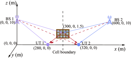
Figure 3: Simulation setup for the RIS-assisted PKG in a two-cell scenario.

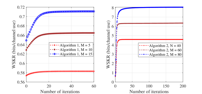
Figure 4: The convergence of Algorithm 1 (left half of the figure) and Algorithm 2 (right half of the figure) for $P_{\rm A}=30$ dBm.

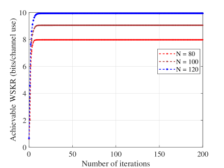
Figure 5: The convergence of the AO algorithm for $M=M_{e}=4$, $P_{\rm A}=30$ dBm.

First, Fig. 4 shows the convergence behavior of Algorithm 1 and Algorithm 2, which correspond to the left and right subfigures, respectively. It can be seen that Algorithm 1 and Algorithm 2 converge monotonically for all of the considered values of $M$ and $N$. This verifies the excellent convergence properties of Algorithms 1 and 2. Furthermore, Fig. 5 depicts the achieved WSKR versus the number of AO iterations. As can be observed, the WSKR converges rapidly to stationary values after a few iterations on average. For $N=80$, the proposed algorithm converges after around $19$ iterations on average. For the case with more RIS elements, i.e., $N=100$, the number of iterations required for the convergence is $25$. This is because the solution space is enlarged when more optimization variables are involved and thus more iterations are required for convergence.

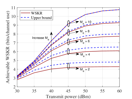
Figure 6: Achievable WSKR versus the transmit power at the BSs, $P_{\rm A}$, for $M=10$ and $N=20$.

Next, in Fig. 6, the WSKR versus the maximum transmit power at each BS for different $M_{e}$ is plotted. First, it can be observed that the WSKRs in all of the settings increase with the transmit power, since the impact of noise becomes insignificant. At the same time, the WSKR increases with diminishing returns at high transmit power region. This is because only the transmit power at the BSs is increased while the power of the UTs is fixed that remains the system performance bottleneck. In particular, the BSs’ channel estimations are still impaired by the noise components, causing the saturation in the WSKR. Furthermore, it can be seen that the WSKR increases with $M_{e}$, since a higher dimensional channel features can be exploited with a larger $M_{e}$. Finally, Fig. 6 shows the tightness of the derived upper bound. Specifically, the performance gap between WSKR and the upper bound is reduced with $M_{e}$ increasing and becomes exact when $M_{e}=M$. This is because having a larger $M_{e}$, the dimension of ${\mathbf{P}}_{k}{\mathbf{z}}_{k}$ approaches that of ${\mathbf{z}}_{k}$. Thus, the upper bound $\mathcal{I}({\mathbf{y}}_{k};{\mathbf{P}}_{k}{\mathbf{z}}_{k})$ becomes tight and accurate in describing $\mathcal{I}({\mathbf{y}}_{k};{\mathbf{z}}_{k})$ such that the proposed design is effective.

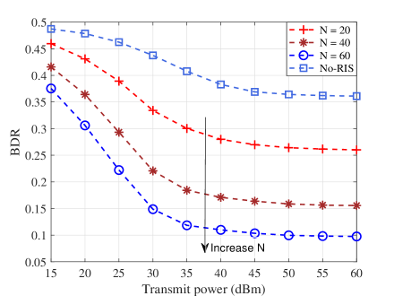
Figure 7: BDR versus the transmit power $P_{\rm A}$ for $M=M_{e}=4$.

To illustrate the impact of the proposed algorithm on the channel reciprocity, we show the BDR result in Fig. 7. The BDR is defined as the ratio between the number of disagreement bits and the number of total bits [2, 5, 6, 7]. It can be seen that the BDR of No-RIS baseline scheme is much higher than the proposed RIS-aided scheme and the former saturates at around $0.36$ BDR in the high transmit power regime. This is because the non-reciprocal interference significantly degrades the similarity of the uplink and downlink channel estimations. In contrast, for the proposed RIS-aided PKG scheme, a lower BDR can be achieved with the increases of RIS elements number $N$, since the RIS is equipped with a higher ability to suppress the pilot contamination-caused inter-cell interference with larger $N$.

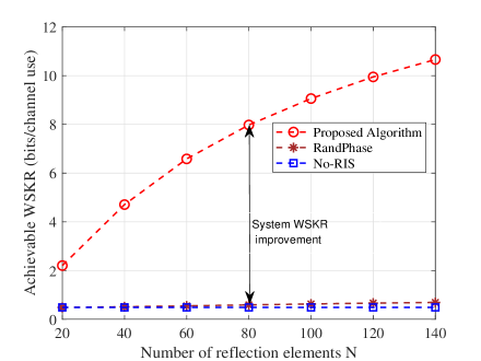
Figure 8: Achievable WSKR versus the number of RIS elements $N$ for $P_{\rm A}=30$ dBm, $M=M_{e}=4$.

Fig. 8 shows the WSKR of different PKG schemes versus the number of RIS elements $N$. Firstly, as can be observed, the WSKRs of the two baseline schemes are significantly low and approach zero. This is because the UTs are located at the cell edge and suffer from severe inter-cell pilot contamination. In contrast, the WSKR of the proposed RIS-based scheme is improved significantly the performance gain increases with the number of RIS elements. This is because the multi-cell interference in the uplink and downlink is eliminated by adjusting the phase shifts of the RIS and with more RIS elements in place, the proposed design becomes more flexible to create pencil-like beams to focus the reflected signals on the target UTs and BSs.

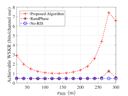
Figure 9: Achievable WSKR versus the location of the RIS $x_{\rm RIS}$ for $M=M_{e}=4$, $N=60$, $P_{\rm A}=30$ dBm.

Fig. 9 presents the WSKR versus the coordinate of the RIS $(x_{\rm RIS},0,0)$. We vary the location of the RIS from near the cell center, $x_{\rm RIS}=20$ m, to the cell boundary, $x_{\rm RIS}=300$ m. It can be observed that the RandPhase baseline scheme achieves its maximum value when the RIS is located near one of the UTs, i.e., $x_{\rm RIS}=280$, which is caused by the array gain brought by the RIS. Also, the proposed algorithm enjoys superior performance than that of the two baseline schemes in all of the considered cases. It is interesting to observe that the WSKR achieved by the proposed algorithm first decreases from $x_{\rm RIS}=20$ to $x_{\rm RIS}=140$, then increases from $x_{\rm RIS}=140$ to $x_{\rm RIS}=280$, and finally decreases from $x_{\rm RIS}=280$ to $x_{\rm RIS}=300$ m. This is mainly caused by the variations of the large-scale fading of the RIS channels. To be specific, the large-scale channel gain of the RIS channel is the product of the gain of the BS-RIS link and that of the RIS-UT link. Thus, for BS $2$ and UT $2$, the large-scale fading of the RIS channels can be approximated by $\zeta_{0}\sqrt{\left((600-x_{\rm RIS})(320-x_{\rm RIS})\right)^{-\alpha_{\rm RIS}}}$, which is negligible for the considered $0\leq x_{\rm RIS}\leq 300$. However, for BS 1 and UT 1, when $0\leq x_{\rm RIS}\leq 280$, the large-scale fading of the RIS channels can be approximated by $\zeta_{0}\sqrt{\left(x_{\rm RIS}(280-x_{\rm RIS})\right)^{-\alpha_{\rm RIS}}}$, which achieves its minimum value at $x_{\rm RIS}=140$ and its maximum value at $x_{\rm RIS}=0$ or $x_{\rm RIS}=280$. This means that the channel gain is minimal when the RIS is located at the middle point between BS 1 and UT 1, while the gain is maximum when the RIS is located close either to BS 1 or UT 1. Furthermore, when the RIS is located away from UT 1, i.e., $280<x_{\rm RIS}\leq 300$, the large-scale fading of the RIS channels between BS $1$ and UT $1$ is given by $\zeta_{0}\sqrt{\left(x_{\rm RIS}(x_{\rm RIS}-280)\right)^{-\alpha_{\rm RIS}}}$, which decreases with an increasing $x_{\rm RIS}$. Additionally, it can be observed from Fig. 9 that the WSKR of deploying the RIS close to the BS, i.e., $x_{\rm RIS}$ approaches $0$, is less than that of deploying near the UT, i.e., $x_{\rm RIS}$ approaches $280$. This is because deploying the RIS close to the cell center is less effective in alleviating the inter-cell pilot contamination.

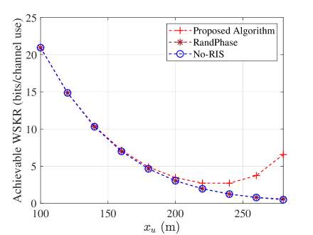
Figure 10: Achievable WSKR versus the location of the RIS $x_{\rm UT}$ for $M=M_{e}=4$, $N=60$, $P_{\rm A}=30$ dBm.

Fig. 10 shows the WSKR versus the location of the UTs under different schemes. The x-coordinates of UT 1 and UT 2 are $x_{u}$ and $600-x_{u}$, respectively. From this figure, the WSKR of all the schemes decrease with $x_{u}$ being from $100$ m to $280$ m. This is mainly due to the following two reasons. First, the channel gain between the BSs and UTs decreases as the UTs move away from their home BSs. Second, the inter-cell interference becomes dominated when the UTs move from the cell center to the cell boundary. However, the proposed RIS-aided PKG scheme provides significant performance gain when the UTs are close to the RIS. Specifically, when $x_{u}=280$ m, the WSKR of the proposed scheme and the two baseline schemes are $6.57$ and $0.49$ bits/channel use, respectively. This is because the UTs receive strong reflected signals from the RIS and the inter-cell interference is substantially mitigated by the RIS.

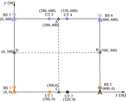
Figure 11: Simulation setup for the RIS-aided PKG in a four-cell scenario.

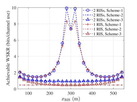
Figure 12: Achievable WSKR versus the location of the RIS $x_{\rm RIS}$ in a four-cell scenario for $M=M_{e}=4$, $P_{\rm A}=30$ dBm.

V-C Four-Cell Scenario

In this section, we consider a four-cell scenario to study the optimal RIS deployment and the impact of having single RIS and multiple RISs on the PKG performance. The coordinates of the four BSs are $(0,0)$, $(600,0)$, $(600,600)$, and $(0,600)$, respectively. The four UTs are located as $(280,0)$, $(320,0)$, $(280,600)$, and $(320,600)$, respectively.

For the single RIS case, we consider 3 schemes: Scheme-1: The RIS moves from BS 1 to BS 2; Scheme-2: The RIS moves from point D to point B; Scheme-3: The RIS moves from BS 3 to BS 2. For the two RISs case, we consider 3 schemes: Scheme-1: RIS 1 moves from BS 1 to BS 2 and RIS 2 moves from BS 3 to BS 4; Scheme-2: RIS 1 moves from BS 1 to BS 4, and RIS 2 moves from BS 3 to BS 2; Scheme-3: RIS 1 moves from point D to point B, and RIS 2 moves from point A to point C.

Fig. 12 shows the WSKR versus the coordinate of the RIS under different schemes. Firstly, for the single-RIS scenario, it is seen that Scheme-1 achieves the maximum WSKR at $x_{\rm RIS}=280$ m and $x_{\rm RIS}=320$ m, which are the locations of UT 1 and UT 2, respectively. This observation is consistent with that of the two-cell system. Additionally, the WSKR of Scheme-1 is significantly higher than that of Scheme-2 and Scheme-3. The reason behind this is the channel gain of the RIS-related channel is higher in Scheme-1 when the RIS is close to the two UTs. Secondly, for the two-RISs scenario, the WSKR curves are similar to that of single-RIS case and the WSKR of Scheme-1 has the maximum value at $x_{\rm RIS}=280$ m and $x_{\rm RIS}=320$ m. The reason is that the RISs are respectively closer to the two of the UTs at these two points. By comparing the WSKR of single-RIS and two-RISs at $x_{\rm RIS}=280$ and $x_{\rm RIS}=320$, we can observe that two-RISs achieve higher performance gain than the single-RIS case. This is because when multiple RISs are deployed in the network, the distance between each UT and its nearest RIS is reduced due to spatial diversity, which thus increases the channel gain. This observation confirms that the PKG performance of the UTs is usually dominated by the closest RIS.

TABLE I: NIST random test result

	Pass ratio	P-value
Approximate entropy	0.9911	0.4851
Runs	0.9985	0.5088
Ranking	0.9941	0.4992
Longest runs of ones	0.9899	0.6238
Frequency	1	0.5201
FFT	0.9853	0.4295
Block frequency	1	0.4401
Cumulative sums	0.9981	0.5057
Serial	0.9838	0.5013, 0.4895

Finally, to verify the randomness of the obtained bit sequences for cryptographic applications, we conduct the National Institute of Standards and Technology (NIST) randomness test [35] on the quantized bits. Note that NIST is widely adopted to evaluate the randomness of true-random and pseudo-random number generators. The output of the NIST is p-values, which is examined to ensure uniformity. The tested sequence is considered to pass the test if the p-value is greater than $0.01$. In the simulation, we perform $9$ kinds of NIST items for $10,000$ trials, with the length of each sequence being $2048$ bits. The test results are shown in Table I, where the pass ratio represents the number of passed trials over the $10,000$ trials. As can be observed, the p-values of all the test items are significantly greater than $0.01$, which means the sequence can be considered to be uniformly distributed. Also, the pass ratios are all higher than 98%. This confirms the excellent randomness of the bits generated by the proposed PKG scheme.

VI Conclusion

In this paper, we incorporated RISs in multi-cell PKG systems to alleviate the negative impact of multi-cell pilot contamination on PKG performance. Specifically, we studied the WSKR maximization problem by jointly optimizing the precoding matrices at the BSs and the phase shifts at the RISs. To tackle this non-convex problem, we derived a tight upper bound of the objective function. To solve the upper bound maximization problem, we applied an AO-based algorithm that alternatively solves the sub-problem for precoding matrices and the sub-problem for phase-shifting vector. In particular, a Lagrangian dual algorithm and a PGA algorithm were employed to design the precoding matrices and the phase-shifting vector, respectively. Simulation results verified the WSKR of the cell edge UTs under multi-cell pilot contamination can be unsatisfactory when the RISs are not deployed. By contrast, the proposed RIS-aided PKG scheme can achieve high WSKR even in harsh channel conditions. Moreover, a lower BDR can be observed with the increase of RIS elements number.

-A Proof of Theorem 1

The KGR between BS $k$ and UT $k$ is expressed as [36], [37]

$$R_{k}=\mathcal{I}({\mathbf{y}}_{k};{\mathbf{z}}_{k})=\ln\frac{\operatorname{det}\left({\mathbf{R}}_{{\mathbf{y}}_{k}}{\mathbf{R}}_{{\mathbf{z}}_{k}}\right)}{\operatorname{det}\left(\mathcal{R}_{{\mathbf{y}}_{k}{\mathbf{z}}_{k}}\right)},$$ (33)

where the covariance matrices are denoted as ${\mathbf{R}}_{{\mathbf{y}}_{k}}=\mathbb{E}\left\{{\mathbf{y}}_{k}{\mathbf{y}}_{k}^{H}\right\}$, ${\mathbf{R}}_{{\mathbf{z}}_{k}}=\mathbb{E}\left\{{\mathbf{z}}_{k}{\mathbf{z}}_{k}^{H}\right\}$, and

$$\mathcal{R}_{{\mathbf{y}}_{k}{\mathbf{z}}_{k}}=\left[\begin{array}[]{ll}{\mathbf{R}}_{{\mathbf{y}}_{k}}&{\mathbf{R}}_{{\mathbf{y}}_{k}{\mathbf{z}}_{k}}\\ {\mathbf{R}}_{{\mathbf{z}}_{k}{\mathbf{y}}_{k}}&{\mathbf{R}}_{{\mathbf{z}}_{k}}\end{array}\right].$$ (36)

Employing the determinant of a block matrix, we have

$$\det\left({\mathbf{R}}_{{\mathbf{y}}_{k}{\mathbf{z}}_{k}}\right)=\det\left({\mathbf{R}}_{{\mathbf{y}}_{k}}\right)\det\left({\mathbf{R}}_{{\mathbf{z}}_{k}}-{\mathbf{R}}_{{\mathbf{z}}_{k}{\mathbf{y}}_{k}}{\mathbf{R}}_{{\mathbf{y}}_{k}}^{-1}{\mathbf{R}}_{{\mathbf{y}}_{k}{\mathbf{z}}_{k}}\right).$$ (37)

Thus, the KGR is reformulated as

$$R_{k} =\ln\left(\frac{\det\left({\mathbf{R}}_{{\mathbf{y}}_{k}}\right)\det\left({\mathbf{R}}_{{\mathbf{z}}_{k}}\right)}{\det\left({\mathbf{R}}_{{\mathbf{y}}_{k}}\right)\det\left({\mathbf{R}}_{{\mathbf{z}}_{k}}-{\mathbf{R}}_{{\mathbf{z}}_{k}{\mathbf{y}}_{k}}{\mathbf{R}}_{{\mathbf{y}}_{k}}^{-1}{\mathbf{R}}_{{\mathbf{y}}_{k}{\mathbf{z}}_{k}}\right)}\right)$$ (38)

$$=-\ln\det\left({\mathbf{I}}-{\mathbf{R}}_{{\mathbf{z}}_{k}{\mathbf{y}}_{k}}{\mathbf{R}}_{{\mathbf{y}}_{k}}^{-1}{\mathbf{R}}_{{\mathbf{y}}_{k}{\mathbf{z}}_{k}}{\mathbf{R}}_{{\mathbf{z}}_{k}}^{-1}\right).$$ (39)

Given the channel estimations in (3) and (6), the channel covariance matrices are calculated as

$${\mathbf{R}}_{{{\mathbf{z}}}_{k}} ={\mathbf{P}}_{k}\left[\sum_{j=1}^{K}{\mathbf{R}}_{k,j}^{d}+\left(\bar{{\mathbf{v}}}^{H}\otimes{\mathbf{I}}_{M}\right)\sum_{j=1}^{K}{\mathbf{R}}_{k,j}^{r}\left(\bar{{\mathbf{v}}}\otimes{\mathbf{I}}_{M}\right)+{\mathbf{I}}_{M}\right]{\mathbf{P}}_{k}^{H},$$ (40)

$${\mathbf{R}}_{{\mathbf{y}}_{k}} =\sum_{i=1}^{K}{\mathbf{P}}_{i}\left({\mathbf{R}}_{i,k}^{d}+\left(\bar{{\mathbf{v}}}^{H}\otimes{\mathbf{I}}_{M}\right){\mathbf{R}}_{i,k}^{r}\left(\bar{{\mathbf{v}}}^{H}\otimes{\mathbf{I}}_{M}\right)^{H}\right){\mathbf{P}}_{i}^{H}+{\mathbf{I}}_{M_{e}},$$ (41)

$${\mathbf{R}}_{{\mathbf{y}}_{k}{{\mathbf{z}}}_{k}} ={\mathbf{P}}_{k}\left({\mathbf{R}}_{k,k}^{d}+\left(\bar{{\mathbf{v}}}^{H}\otimes{\mathbf{I}}_{M}\right){\mathbf{R}}_{k,k}^{r}\left(\bar{{\mathbf{v}}}\otimes{\mathbf{I}}_{M}\right)\right){\mathbf{P}}_{k}^{H}={\mathbf{R}}_{{{\mathbf{z}}}_{k}{\mathbf{y}}_{k}}.$$ (42)

Substituting these channel covariance matrices into (39) and the result follows immediately.

-B Proof of Proposition 1

First, the eigenvalue decomposition of ${\mathbf{R}}^{d}_{i,k}$ can be described as ${\mathbf{Q}}_{\rm D}{\rm{diag}}\left({\mathbf{x}}\right){\mathbf{Q}}_{\rm D}^{H}$, where ${\mathbf{x}}=[x_{1},\cdots,x_{M}]$ is the eigenvalue vector and ${\mathbf{Q}}_{\rm D}=\left[{\mathbf{c}}_{1},\cdots,{\mathbf{c}}_{M}\right]$ is the eigenmatrix and ${\mathbf{c}}_{\ell},\ell\in\left\{1,\cdots,M\right\}$, is the eigenvector. By denoting $\sum_{j=1}^{K}{\mathbf{R}}^{d}_{k,j}+{\mathbf{I}}_{M}={\mathbf{A}}$ and $P_{i}\sum_{i=1}^{K}{\mathbf{R}}^{d}_{i,k}+{\mathbf{I}}_{M}={\mathbf{B}}$, the derivative of $R_{k}$ w.r.t. $x_{\ell},\ell\in\left\{1,\cdots,M\right\}$, is

$$\partial R_{k}/\partial x_{\ell}=-{\rm{tr}}\left({\mathbf{B}}^{-1}{\mathbf{R}}^{d}_{k,k}\left({\mathbf{A}}-P_{k}{\mathbf{R}}^{d}_{k,k}{\mathbf{B}}^{-1}{\mathbf{R}}^{d}_{k,k}\right)^{-1}P_{k}{\mathbf{R}}^{d}_{k,k}{\mathbf{B}}^{-1}P_{i}{\mathbf{c}}_{\ell}{\mathbf{c}}_{\ell}^{H}\right).$$ (43)

Since ${\mathbf{A}}-P_{k}{\mathbf{R}}^{d}_{k,k}{\mathbf{B}}^{-1}{\mathbf{R}}^{d}_{k,k}\succ{\mathbf{0}}$ and ${\mathbf{c}}_{\ell}{\mathbf{c}}_{\ell}^{H}\succeq{\mathbf{0}}$, we have $\partial R_{k}/\partial x_{\ell}<0$. Thus, $R_{k}$ decreases monotonically with $x_{\ell}$. When $\lambda_{\ell}\left({\mathbf{R}}^{d}_{i,k}\right)\rightarrow\infty$, we have $\lambda_{\ell}\left(\sum_{i=1}^{K}P_{i}{\mathbf{R}}^{d}_{i,k}+{\mathbf{I}}_{M}\right)\rightarrow 0$, and thus $R_{k}\rightarrow 0$. The proof for ${\mathbf{R}}^{d}_{k,j}$ and $P_{i}$ can be derived similarly. This completes the poof.

-C Proof of Theorem 2

According to the data-processing inequality, we have $\mathcal{I}({\mathbf{y}}_{k};{\mathbf{z}}_{k})\leq\mathcal{I}({\mathbf{y}}_{k};\tilde{{\mathbf{z}}}_{k})$. Next, we calculate the mutual information $I({\mathbf{y}}_{k};\tilde{{\mathbf{z}}}_{k})$. The channel covariance matrices are calculated as

$${\mathbf{R}}_{\tilde{{\mathbf{z}}}_{k}} =\sum_{j=1}^{K}{\mathbf{R}}_{k,j}^{d}+\left(\bar{{\mathbf{v}}}^{H}\otimes{\mathbf{I}}_{M}\right)\sum_{j=1}^{K}{\mathbf{R}}_{k,j}^{r}\left(\bar{{\mathbf{v}}}\otimes{\mathbf{I}}_{M}\right)+{\mathbf{I}}_{M},$$ (44)

$${\mathbf{R}}_{{\mathbf{y}}_{k}} =\sum_{i=1}^{K}{\mathbf{P}}_{i}\left({\mathbf{R}}_{i,k}^{d}+\left(\bar{{\mathbf{v}}}^{H}\otimes{\mathbf{I}}_{M}\right){\mathbf{R}}_{i,k}^{r}\left(\bar{{\mathbf{v}}}^{H}\otimes{\mathbf{I}}_{M}\right)^{H}\right){\mathbf{P}}_{i}^{H}+{\mathbf{I}}_{M_{e}},$$ (45)

$${\mathbf{R}}_{{\mathbf{y}}_{k}\tilde{{\mathbf{z}}}_{k}} ={\mathbf{P}}_{k}\left({\mathbf{R}}_{k,k}^{d}+\left(\bar{{\mathbf{v}}}^{H}\otimes{\mathbf{I}}_{M}\right){\mathbf{R}}_{k,k}^{r}\left(\bar{{\mathbf{v}}}\otimes{\mathbf{I}}_{M}\right)\right),$$ (46)

$${\mathbf{R}}_{\tilde{{\mathbf{z}}}_{k}{\mathbf{y}}_{k}} =\left({\mathbf{R}}_{k,k}^{d}+\left(\bar{{\mathbf{v}}}^{H}\otimes{\mathbf{I}}_{M}\right){\mathbf{R}}_{k,k}^{r}\left(\bar{{\mathbf{v}}}\otimes{\mathbf{I}}_{M}\right)\right){\mathbf{P}}_{k}^{H}.$$ (47)

Substituting these channel covariance matrices into (39), the upper bound of the KGR is expressed as (11). This completes the proof.

-D Proof of Theorem 3

We can calculate the conjugate gradient of $\mathcal{L}\left({\mathbf{P}},{{\mathbf{\Lambda}}}\right)$ w.r.t. ${\mathbf{P}}$ as

$$\frac{\partial\mathcal{L}\left({\mathbf{P}},{{\mathbf{\Lambda}}}\right)}{\partial{\mathbf{P}}^{*}} =\sum_{k=1}^{K}w_{k}\left(\left({\mathbf{P}}{\mathbf{M}}_{k}{\mathbf{P}}^{H}+{\mathbf{I}}_{M_{e}}\right)^{-1}{\mathbf{P}}{\mathbf{M}}_{k}-\left({\mathbf{P}}{\mathbf{N}}_{k}{\mathbf{P}}^{H}+{\mathbf{I}}_{M_{e}}\right)^{-1}{\mathbf{P}}{\mathbf{N}}_{k}\right)-{\mathbf{P}}{{\mathbf{\Lambda}}}.$$ (48)

Set $\frac{\partial\mathcal{L}\left({\mathbf{P}},{{\mathbf{\Lambda}}}\right)}{\partial{\mathbf{P}}^{*}}={\mathbf{0}}$ and take the $\text{vec}(\cdot)$ operation on the both sides of the equation, we can obtain the KKT condition as shown in (17). This completes the proof.

-E Proof of Theorem 4

First, the upper bound is given by

$$R_{k}^{\rm ub} =\ln\det\left({\mathbf{R}}_{{\mathbf{y}}_{k}}\right)-\ln\det\left({\mathbf{R}}_{{\mathbf{y}}_{k}}-{\mathbf{R}}_{{\mathbf{y}}_{k}\tilde{{\mathbf{z}}}_{k}}{\mathbf{R}}_{\tilde{{\mathbf{z}}}_{k}}^{-1}{\mathbf{R}}_{\tilde{{\mathbf{z}}}_{k}{\mathbf{y}}_{k}}\right)$$ (49)

and the differential of $R_{k}^{\rm ub}$ w.r.t. $\bar{{\mathbf{v}}}$ is written as

$$d\left(R_{k}^{\rm ub}\right) ={\rm{tr}}\left({\mathbf{R}}_{{\mathbf{y}}_{k}}^{-1}d\left({\mathbf{R}}_{{\mathbf{y}}_{k}}\right)\right)-{\rm{tr}}\left(\left({\mathbf{R}}_{{\mathbf{y}}_{k}}-{\mathbf{R}}_{{\mathbf{y}}_{k}\tilde{{\mathbf{z}}}_{k}}{\mathbf{R}}_{\tilde{{\mathbf{z}}}_{k}}^{-1}{\mathbf{R}}_{\tilde{{\mathbf{z}}}_{k}{\mathbf{y}}_{k}}\right)^{-1}d\left({\mathbf{R}}_{{\mathbf{y}}_{k}}-{\mathbf{R}}_{{\mathbf{y}}_{k}\tilde{{\mathbf{z}}}_{k}}{\mathbf{R}}_{\tilde{{\mathbf{z}}}_{k}}^{-1}{\mathbf{R}}_{\tilde{{\mathbf{z}}}_{k}{\mathbf{y}}_{k}}\right)\right).$$ (50)

Then, the first term of (50) is calculated as

$${\rm{tr}}\left({\mathbf{R}}_{{\mathbf{y}}_{k}}^{-1}d\left({\mathbf{R}}_{{\mathbf{y}}_{k}}\right)\right) ={\rm{tr}}\left({{\mathbf{K}}_{M_{e}NL}\sum_{i=1}^{K}\left({\mathbf{I}}_{NL}\otimes{\mathbf{P}}_{i}\right){\mathbf{R}}_{i,k}^{r}\left({\mathbf{I}}_{NL}\otimes{\mathbf{P}}_{i}\right)^{H}\left(\bar{{\mathbf{v}}}\otimes{\mathbf{I}}_{M_{e}}\right){\mathbf{R}}_{{\mathbf{y}}_{k}}^{-1}{\mathbf{K}}_{M_{e}}}{\left({\mathbf{I}}_{M_{e}}\otimes d\left(\bar{{\mathbf{v}}}^{H}\right)\right)}\right).$$ (51)

Similarly, we can calculate the second term of (50) as

$$\quad{\rm{tr}}\left(\left({\mathbf{R}}_{{\mathbf{y}}_{k}}-{\mathbf{R}}_{{\mathbf{y}}_{k}\tilde{{\mathbf{z}}}_{k}}{\mathbf{R}}_{\tilde{{\mathbf{z}}}_{k}}^{-1}{\mathbf{R}}_{\tilde{{\mathbf{z}}}_{k}{\mathbf{y}}_{k}}\right)^{-1}d\left({\mathbf{R}}_{{\mathbf{y}}_{k}}-{\mathbf{R}}_{{\mathbf{y}}_{k}\tilde{{\mathbf{z}}}_{k}}{\mathbf{R}}_{\tilde{{\mathbf{z}}}_{k}}^{-1}{\mathbf{R}}_{\tilde{{\mathbf{z}}}_{k}{\mathbf{y}}_{k}}\right)\right)$$ (52)

$$={\rm{tr}}\left({{\mathbf{K}}_{M_{e}NL}\sum_{i=1}^{K}\left({\mathbf{I}}_{NL}\otimes{\mathbf{P}}_{i}\right){\mathbf{R}}_{i,k}^{r}\left({\mathbf{I}}_{NL}\otimes{\mathbf{P}}_{i}\right)^{H}\left(\bar{{\mathbf{v}}}\otimes{\mathbf{I}}_{M_{e}}\right)\left({\mathbf{R}}_{{\mathbf{y}}_{k}}-{\mathbf{R}}_{{\mathbf{y}}_{k}\tilde{{\mathbf{z}}}_{k}}{\mathbf{R}}_{\tilde{{\mathbf{z}}}_{k}}^{-1}{\mathbf{R}}_{\tilde{{\mathbf{z}}}_{k}{\mathbf{y}}_{k}}\right)^{-1}{\mathbf{K}}_{M_{e}}}{\left({\mathbf{I}}_{M_{e}}\otimes d\left(\bar{{\mathbf{v}}}^{H}\right)\right)}\right)$$

$$\quad-{\rm{tr}}\left({\mathbf{R}}_{\tilde{{\mathbf{z}}}_{k}}^{-1}{\mathbf{R}}_{\tilde{{\mathbf{z}}}_{k}{\mathbf{y}}_{k}}\left({\mathbf{R}}_{{\mathbf{y}}_{k}}-{\mathbf{R}}_{{\mathbf{y}}_{k}\tilde{{\mathbf{z}}}_{k}}{\mathbf{R}}_{\tilde{{\mathbf{z}}}_{k}}^{-1}{\mathbf{R}}_{\tilde{{\mathbf{z}}}_{k}{\mathbf{y}}_{k}}\right)^{-1}{d\left({\mathbf{R}}_{{\mathbf{y}}_{k}\tilde{{\mathbf{z}}}_{k}}\right)}\right)$$

$$\quad-{\rm{tr}}\left({\mathbf{R}}_{\tilde{{\mathbf{z}}}_{k}{\mathbf{y}}_{k}}\left({\mathbf{R}}_{{\mathbf{y}}_{k}}-{\mathbf{R}}_{{\mathbf{y}}_{k}\tilde{{\mathbf{z}}}_{k}}{\mathbf{R}}_{\tilde{{\mathbf{z}}}_{k}}^{-1}{\mathbf{R}}_{\tilde{{\mathbf{z}}}_{k}{\mathbf{y}}_{k}}\right)^{-1}{\mathbf{R}}_{{\mathbf{y}}_{k}\tilde{{\mathbf{z}}}_{k}}{d\left({\mathbf{R}}_{\tilde{{\mathbf{z}}}_{k}}^{-1}\right)}\right)$$

$$\quad-{\rm{tr}}\left(\left({\mathbf{R}}_{{\mathbf{y}}_{k}}-{\mathbf{R}}_{{\mathbf{y}}_{k}\tilde{{\mathbf{z}}}_{k}}{\mathbf{R}}_{\tilde{{\mathbf{z}}}_{k}}^{-1}{\mathbf{R}}_{\tilde{{\mathbf{z}}}_{k}{\mathbf{y}}_{k}}\right)^{-1}{\mathbf{R}}_{{\mathbf{y}}_{k}\tilde{{\mathbf{z}}}_{k}}{\mathbf{R}}_{\tilde{{\mathbf{z}}}_{k}}^{-1}{d\left({\mathbf{R}}_{\tilde{{\mathbf{z}}}_{k}{\mathbf{y}}_{k}}\right)}\right).$$ (53)

By calculating each differential term in (53), we can obtain

$$d\left(R_{k}^{\rm ub}\right)={\rm{tr}}\left({\mathbf{G}}_{k}d\left({\mathbf{I}}_{M}\otimes d\left(\bar{{\mathbf{v}}}^{H}\right)\right)\right)+{\rm{tr}}\left({\mathbf{Q}}_{k}d\left({\mathbf{I}}_{M_{e}}\otimes d\left(\bar{{\mathbf{v}}}^{H}\right)\right)\right).$$ (54)

Therefore, the conjugate gradient of $R_{k}^{\rm ub}$ w.r.t. $\bar{{\mathbf{v}}}$ is calculated as

$$\frac{\partial R_{k}^{\rm ub}}{\partial\bar{{\mathbf{v}}}^{*}}=\sum_{m=1}^{M_{e}}\bar{{\mathbf{q}}}_{k,m}+\sum_{m=1}^{M}\bar{{\mathbf{g}}}_{k,m}.$$ (55)

This completes the proof.

References

• [1] M. Ylianttila, R. Kantola, A. V. Gurtov, and et al., “6G white paper: Research challenges for trust, security and privacy,” arXiv:2004.11665, 2020. [Online]. Available: https://arxiv.org/abs/2004.11665
• [2] J. Zhang, T. Q. Duong, A. Marshall, and R. Woods, “Key generation from wireless channels: A review,” IEEE Access, vol. 4, no. 3, pp. 614–626, Jan. 2017.
• [3] L. Jiao, N. Wang, P. Wang, A. Alipour-Fanid, J. Tang, and K. Zeng, “Physical layer key generation in 5G wireless networks,” IEEE Wireless Commun. Mag., vol. 26, no. 5, pp. 48–54, Oct. 2019.
• [4] U. M. Maurer, “Secret key agreement by public discussion from common information,” IEEE Trans. Inf. Theory, vol. 39, no. 3, pp. 733–742, May 1993.
• [5] R. Guillaume, F. Winzer, A. Czylwik, and et al., “Bringing phy-based key generation into the field: An evaluation for practical scenarios,” in Proc. IEEE 82nd Veh. Technol. Conf. (VTC-Fall), Boston, MA, USA, Sept. 2015, pp. 1–5.
• [6] G. Li, C. Sun, E. A. Jorswieck, and et al., “Sum secret key rate maximization for TDD multi-user massive MIMO wireless networks,” IEEE Trans. Inf. Forensics Security, vol. 16, pp. 968–982, Sept. 2021.
• [7] S. Mathur, W. Trappe, N. Mandayam, and et al., “Radio-telepathy: extracting a secret key from an unauthenticated wireless channel,” in Proc. 14th Annu. Int. Conf. Mobile Computing and Networking (MobiCom), San Francisco, California, USA, Sept. 2008, pp. 128–139.
• [8] G. Li, L. Hu, P. Staat, H. Elders-Boll, C. Zenger, C. Paar, and A. Hu, “Reconfigurable intelligent surface for physical layer key generation: Constructive or destructive?” IEEE Wireless Commun. Mag., pp. 1–12, May 2022.
• [9] G. Li, C. Sun, W. Xu, M. D. Renzo, and A. Hu, “On maximizing the sum secret key rate for reconfigurable intelligent surface-assisted multiuser systems,” IEEE Tran. Inf. Forensics Security, vol. 17, pp. 211–225, Dec. 2022.
• [10] X. Yu, V. Jamali, D. Xu, D. W. K. Ng, and R. Schober, “Smart and reconfigurable wireless communications: From IRS modeling to algorithm design,” IEEE Wireless Commun. Mag., vol. 28, no. 6, pp. 118–125, Dec. 2021.
• [11] M. Di Renzo, K. Ntontin, J. Song, and et al., “Reconfigurable intelligent surfaces vs. relaying: Differences, similarities, and performance comparison,” IEEE Open Journal of the Communications Society, vol. 1, pp. 798–807, Jun. 2020.
• [12] C. Pan, H. Ren, K. Wang, and et al., “Reconfigurable intelligent surfaces for 6G systems: Principles, applications, and research directions,” IEEE Commun. Mag., vol. 59, no. 6, pp. 14–20, Jul. 2021.
• [13] X. Lu, J. Lei, Y. Shi, and W. Li, “Intelligent reflecting surface assisted secret key generation,” IEEE Signal Process. Lett., vol. 28, pp. 1036–1040, Feb. 2021.
• [14] Z. Ji, P. L. Yeoh, D. Zhang, and et al., “Secret key generation for intelligent reflecting surface assisted wireless communication networks,” IEEE Trans. Veh. Technol., vol. 70, no. 1, pp. 1030–1034, Dec. 2021.
• [15] L. Hu, G. Li, X. Qian, A. Hu, and D. W. K. Ng, “Reconfigurable intelligent surface-assisted secret key generation in spatially correlated channels,” arXiv:2211.03132, 2022. [Online]. Available: https://arxiv.org/abs/2211.03132
• [16] T. Lu, L. Chen, J. Zhang, C. Chen, and A. Hu, “Joint precoding and phase shift design in reconfigurable intelligent surfaces-assisted secret key generation,” arXiv:2208.00218, 2022. [Online]. Available: https://arxiv.org/abs/2208.00218
• [17] C. Chen, J. Zhang, T. Lu, M. Sandell, and L. Chen, “Machine learning-based secret key generation for IRS-assisted multi-antenna systems,” arXiv:2301.08179, 2022. [Online]. Available: https://arxiv.org/abs/2301.08179
• [18] J. Jose, A. Ashikhmin, T. L. Marzetta, and S. Vishwanath, “Pilot contamination problem in multi-cell TDD systems,” in Proc. IEEE Int. Symp. Inf. Theory (ISIT), Seoul, Korea, Jun. 2009, pp. 2184–2188.
• [19] H. Yin, L. Cottatellucci, D. Gesbert, R. R. Müller, and G. He, “Robust pilot decontamination based on joint angle and power domain discrimination,” IEEE Trans. Signal Process., vol. 64, no. 11, pp. 2990–3003, Feb. 2016.
• [20] J. Jose, A. Ashikhmin, T. L. Marzetta, and S. Vishwanath, “Pilot contamination and precoding in multi-cell TDD systems,” IEEE Trans. Wireless Commun., vol. 10, no. 8, pp. 2640–2651, Aug. 2011.
• [21] H. Q. Ngo and E. G. Larsson, “EVD-based channel estimation in multicell multiuser MIMO systems with very large antenna arrays,” in Proc. IEEE Int. Conf. Acoust., Speech Signal Process. (ICASSP), Kyoto, Japan, Mar. 2012, pp. 3249–3252.
• [22] R. R. Müller, L. Cottatellucci, and M. Vehkaperä, “Blind pilot decontamination,” IEEE J. Sel. Topics in Signal Processing, vol. 8, no. 5, pp. 773–786, Oct. 2014.
• [23] D. Hu, L. He, and X. Wang, “Semi-blind pilot decontamination for massive MIMO systems,” IEEE Trans. Wireless Commun., vol. 15, no. 1, pp. 525–536, Sep. 2016.
• [24] H. Yin, D. Gesbert, M. Filippou, and Y. Liu, “A coordinated approach to channel estimation in large-scale multiple-antenna systems,” IEEE J. Sel. Areas Commun., vol. 31, no. 2, pp. 264–273, Jan. 2013.
• [25] Q. Wu and R. Zhang, “Towards smart and reconfigurable environment: Intelligent reflecting surface aided wireless network,” IEEE Commun. Mag., vol. 58, no. 1, pp. 106–112, Jan. 2019.
• [26] G. Yang, H. Zhang, Z. Shi, S. Ma, and H. Wang, “Asymptotic outage analysis of spatially correlated Rayleigh MIMO channels,” IEEE Trans. Broadcast, vol. 67, no. 1, pp. 263–278, Oct. 2020.
• [27] C. Sun and G. Li, “Power allocation and beam scheduling for multi-user massive MIMO secret key generation,” IEEE Access, vol. 8, pp. 164 580–164 592, Sep. 2020.
• [28] J. W. Wallace, C. Chen, and M. A. Jensen, “Key generation exploiting MIMO channel evolution: Algorithms and theoretical limits,” in Proc. European Conference on Antennas & Propagation, Berlin, Germany, Jun. 2009, pp. 1–5.
• [29] X. Yu, D. Xu, Y. Sun, D. W. K. Ng, and R. Schober, “Robust and secure wireless communications via intelligent reflecting surfaces,” IEEE J. Sel. Areas Commun., vol. 38, no. 11, pp. 2637–2652, Jul. 2020.
• [30] S. Bubeck, “Convex optimization: Algorithms and complexity,” Found. Trends Mach. Learn., vol. 8, no. 3-4, pp. 231–357, 2015.
• [31] T. M. Cover, Elements of information theory.   John Wiley & Sons, 1999.
• [32] A. Papazafeiropoulos, C. Pan, P. Kourtessis, S. Chatzinotas, and J. M. Senior, “Intelligent reflecting surface-assisted mu-miso systems with imperfect hardware: Channel estimation and beamforming design,” IEEE Trans. Wireless Commun., vol. 21, no. 3, pp. 2077–2092, Sep. 2022.
• [33] X.-D. Zhang, Matrix analysis and applications.   Cambridge University Press, 2017.
• [34] C. Pan, H. Ren, K. Wang, W. Xu, M. Elkashlan, A. Nallanathan, and L. Hanzo, “Multicell MIMO communications relying on intelligent reflecting surfaces,” IEEE Trans. Wireless Commun., vol. 19, no. 8, pp. 5218–5233, May 2020.
• [35] A. Rukhin, J. Soto, J. Nechvatal, M. Smid, and E. Barker, “A statistical test suite for random and pseudorandom number generators for cryptographic applications,” DTIC Document, Tech. Rep., 2001.
• [36] E. A. Jorswieck, A. Wolf, and S. Engelmann, “Secret key generation from reciprocal spatially correlated MIMO channels,” in Proc. IEEE Globecom Workshops (GC Wkshps), Atlanta, USA, Dec. 2013, pp. 1245–1250.
• [37] T. F. Wong, M. Bloch, and J. M. Shea, “Secret sharing over fast-fading MIMO wiretap channels,” EURASIP J. Wirel. Comm., vol. 2009, pp. 1–17, 2009.