$\mathcal{C}^{k}$-continuous Spline Approximation with TensorFlow Gradient Descent Optimizers

Abstract

In this work we present an “out-of-the-box” application of Machine Learning (ML) optimizers for an industrial optimization problem. We introduce a piecewise polynomial model (spline) for fitting of $\mathcal{C}^{k}$-continuos functions, which can be deployed in a cam approximation setting. We then use the gradient descent optimization context provided by the machine learning framework TensorFlow to optimize the model parameters with respect to approximation quality and $\mathcal{C}^{k}$-continuity and evaluate available optimizers. Our experiments show that the problem solution is feasible using TensorFlow gradient tapes and that AMSGrad and SGD show the best results among available TensorFlow optimizers. Furthermore, we introduce a novel regularization approach to improve SGD convergence. Although experiments show that remaining discontinuities after optimization are small, we can eliminate these errors using a presented algorithm which has impact only on affected derivatives in the local spline segment.

1 Introduction

When discussing the potential application of Machine Learning (ML) to industrial settings, we first of all have the application of various ML methods and models per se in mind. These methods, from neural networks to simple linear classifiers, are based on gradient descent optimization. This is why ML frameworks come with a variety of gradient descent optimizers that perform well on a diverse set of problems and in the past decades have received significant improvements in academia and practice.

Industry is full of classical numerical optimization and we can therefore, instead of using the entire framework in an industrial context, harness modern optimizers that lie at the heart of modern ML methods directly and apply them to industrial numerical optimization tasks. One of these optimization tasks is cam approximation, which is the task of fitting a continuous function to a number of input points with properties favorable for cam design. One way to achieve these favorable properties is via gradient based approaches, where an objective function allows to minimize user-definable losses. Servo drives like B&R Industrial Automation’s ACOPOS series process cam profiles as a piecewise polynomial function (spline). This is why, with the goal of using the findings of this paper as a basis for cam approximation in future works, we want to lay the ground for performing polynomial approximation with a $\mathcal{C}^{k}$-continuous piecewise polynomial spline model using gradient descent optimization provided by the machine learning framework TensorFlow. The continuity class $\mathcal{C}^{k}$ denotes the set of $k$-times continuously differentiable functions $\mathbb{R}\to\mathbb{R}$. Continuity is important in cam design concerning forces that are only constrained by the mechanical construction of machine parts. This leads to excessive wear and vibrations which we ought to prevent. Although our approach is motivated by cam design, it is generically applicable.

The contribution of this work is manifold:

1. “Out-of-the-box” application of ML-optimizers for an industrial setting.

2. A $\mathcal{C}^{k}$-spline approximation method with novel gradient regularization.

3. Evaluation of TensorFlow optimizer performance for a well-known problem.

4. Non-convergence of optimizers using exponential moving averages, like Adam, is documented in literature [2]. We confirm with our experiments that this non-convergence extends to the presented optimization setting.

5. Algorithm to strictly establish continuity with impact only on affected derivatives in the local spline segment.

The Python libraries and Jupyter Notebooks used to perform our experiments are available under an MIT license at [5].

Prior work

There is a lot of prior work on neural networks for function approximation [1] or the use of gradient descent optimizers for B-spline curves [3]. There are also non-scientific texts on gradient descent optimization for polynomial regression. However, to the best of our knowledge, there is no thorough evaluation of gradient descent optimizers for $\mathcal{C}^{k}$-continuous piecewise polynomial spline approximation.

2 Gradient descent optimization

TensorFlow provides a mechanism for automatic gradient computation using a so-called gradient tape. This mechanism allows to directly make use of the diverse range of gradient based optimizers offered by the framework and implement custom training loops. We implemented our own training loop in which we (i) obtain the gradients for a loss expression $\ell$, (ii) optionally apply some regularization on the gradients and (iii) supply the optimizer with the gradients. This requires a computation of $\ell$ that allows the gradient tape to track the operations applied to the model parameters in form of TensorFlow variables.

2.1 Spline model

Many servo drives used in industrial applications, like B&R Industrial Automation’s ACOPOS series, use piecewise polynomial functions (splines) as a base model for cam follower displacement curves. This requires the introduction of an according spline model in TensorFlow. Let us consider $n$ samples at $x_{1}\leq\dots\leq x_{n}\in\mathbb{R}$ with respective values $y_{i}\in\mathbb{R}$. We ask for a spline $f\colon I\to\mathbb{R}$ on the interval $I=[x_{1},x_{n}]$ that approximates the samples well and fulfills some additional domain-specific properties, like $\mathcal{C}^{k}$-continuity or $\mathcal{C}^{k}$-cyclicity. Let us denote by $\xi_{0}\leq\dots\leq\xi_{m}$ the polynomial boundaries of $f$, where $\xi_{0}=x_{1}$ and $\xi_{m}=x_{n}$. With $I_{i}=[\xi_{i-1},\xi_{i}]$, the spline $f$ is modeled by $m$ polynomials $p_{i}\colon I\to\mathbb{R}$ that agree with $f$ on $I_{i}$ for $1\leq i\leq m$. Each polynomial

$$p_{i}=\sum_{j=0}^{d}\alpha_{i,j}x^{j}$$ (1)

is determined by its coefficients $\alpha_{i,j}$, where $d$ denotes the degree of the spline and its polynomials. That is, the $\alpha_{i,j}$ are the to be trained model parameters of the spline ML model. We investigate the convergence of these model parameters $\alpha_{i,j}$ of this spline model with respect to different loss functions, specifically for $L_{2}$-approximation error and $\mathcal{C}^{k}$-continuity, by means of different TensorFlow optimizers (see details below). Figure 1 depicts the principles of the presented spline model.

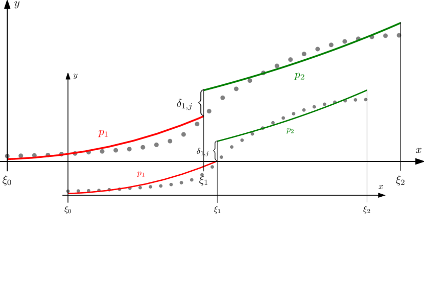
Figure 1: Spline model derivative $j$ consisting of two polynomial segments.

2.2 Loss Function

In order to establish $\mathcal{C}^{k}$-continuity, cyclicity, periodicity and allow for curve fitting via least squares approximation, we introduce the cost function

$$\ell=\lambda\ell_{2}+(1-\lambda)\ell_{\text{CK}}.$$ (2)

By adjusting the value of $\lambda$ in equation (2) we can put more weight to either the approximation quality or $\mathcal{C}^{k}$-continuity optimization target. The approximation error $\ell_{2}$ is the least-square error and made invariant to the number of data points and number of polynomial segments by the following definition:

$$\ell_{2}=\frac{m}{n}\sum_{i}|f(x_{i})-y_{i}|^{2}.$$ (3)

We assign a value $\ell_{\text{CK}}$ to the amount of discontinuity in our spline function by summing up discontinuities at all $\xi_{i}$ across relevant derivatives as

$$\ell_{\text{CK}}=\frac{1}{m-1}\sum_{i=1}^{m-1}\sum_{j=0}^{k}\delta_{i,j}^{2}\quad\text{with}\quad\delta_{i,j}=p^{(j)}_{i+1}(\xi_{i})-p^{(j)}_{i}(\xi_{i}).$$ (4)

We make $\ell_{\text{CK}}$ in equation (4) invariant to the number of polynomial segments by applying an equilibration factor $\frac{1}{m-1}$, where $m-1$ is the number of boundary points excluding $\xi_{0}$ and $\xi_{m}$. This loss $\ell_{\text{CK}}$ can be naturally extended to $\mathcal{C}^{k}$-cyclicity/periodicity for cam profiles.

2.3 TensorFlow Training Loop

The gradient tape environment of TensorFlow offers automatic differentiation of our loss function defined in equation (2). This requires a computation of $\ell$ that allows for tracking the operations applied to $\alpha_{i,j}$ through the usage of TensorFlow variables and arithmetic operations, see Listing LABEL:lst:optimization_loop.

In this training loop, we first calculate the loss according to equation (2) in a gradient tape context in lines 5 and 6 and then obtain the gradients according to that loss result in line 7 via the gradient tape environment automatic differentiation mechanism. We then apply regularization in line 8 that later will be introduced in section 3.1 and supply the optimizer with the gradients in line 9.

⬇

1 for e in range(epochs):

2 with tf.GradientTape(persistent=True) as tape:

3 loss_l2 = calculate_l2_loss()

4 loss_ck = calculate_ck_loss()

5 loss = tf.add(tf.multiply(loss_l2, lambd),

6 tf.multiply(loss_ck, 1.0-lambd))

7 gradients = tape.gradient(loss, coeffs)

8 gradients = apply_regularization()

9 optimizer.apply_gradients(zip(gradients, coeffs))

Listing 1: Gradient descent optimization loop in TensorFlow.

3 Improving spline model performance

In order to improve convergence behavior using the model defined in section 2.1, we introduce a novel regularization approach and investigate effects of input data scaling and shifting of polynomial centers. In a cam design context, discontinuities remaining after the optimization procedure lead to forces and vibrations that are only constrained by the cam-follower system’s mechanical design. To prevent such discontinuities, we propose an algorithm to strictly establish continuity after optimization.

3.1 A degree-based regularization

With the polynomial model described in equation (1), terms of higher order have greater impact on the result. This leads to gradients having greater impact on terms of higher order, which impairs convergence behavior. This effect is also confirmed by our experiments. We propose a degree-based regularization approach, that mitigates this impact by effectively causing a shift of optimization of higher-degree coefficients to later epochs. We do this by introducing a gradient regularization vector $R=(r_{0},\dots,r_{d})$, where

$$r_{j}=\frac{r^{\prime}_{j}}{\sum_{k=0}^{d}r^{\prime}_{k}}\quad\text{with}\quad r^{\prime}_{j}=\frac{1}{1+j}.$$ (5)

The regularization is then applied by multiplying each gradient value $\pdv{\ell}{\alpha_{i,j}}$ with $r_{j}$. Since the entries $r_{j}$ of $R$ sum up to $1$, this effectively acts as an equilibration of all gradients per polynomial $p_{i}$.

This approach effectively makes the sum of gradients degree-independent. Experiments show that this allows for higher learning rates using non-adaptive optimizers like SGD and enables the use of SGD with Nesterov momentum, which does not converge without our proposed regularization approach. This brings faster convergence rates and lower remaining losses for non-adaptive optimizers. At a higher number of epochs, the advantage of the regularization is becoming less. Also, the advantage of the regularization is higher for polynomials of higher degree, say, $d\geq 4$.

3.2 Practical considerations

Experiments show that, using the training parameters outlined in chapter 4, SGD optimization has a certain radius of convergence with respect to the $x$-axis around the polynomial center. Shifting of polynomial centers to the mean of the respective segment allows segments with higher $x$-value ranges to converge. We can implement this by extending the polynomial model defined in equation (1) as

$$p_{i}=\sum_{j=0}^{d}\alpha_{i,j}(x-\mu_{i})^{j},\quad\text{where}\quad\mu_{i}=\frac{\xi_{i-1}+\xi_{i}}{2}.$$ (6)

If input data is scaled such that every polynomial segment is in the range $[0,1]$, in all our experiments for all $0\leq\lambda\leq 1$, SGD optimization is able to converge using this approach. With regards to scaling, as an example, for a spline consisting of $8$ polynomial segments, we scale the input data such that $I=[0,8]$. We skip the back-transformation as we would do in production code.

3.3 Strictly establishing continuity after optimization

In order to strictly establish $\mathcal{C}^{k}$-continuity after optimization, i.e., to eliminate possible remaining $\ell_{\text{CK}}$, we apply corrective polynomials that enforce $\delta(\xi_{i})=0$ at all $\xi_{i}$. The following method requires a spline degree $d\geq 2k+1$. Let

$$m_{i,j}=\frac{p^{(j)}_{i}(\xi_{i})+p^{(j)}_{i+1}(\xi_{i})}{2}$$ (7)

denote the mean $j$-th derivative of $p_{i}$ and $p_{i+1}$ at $\xi_{i}$ for all $0\leq j\leq k$. Then there is a unique polynomial $c_{i}$ of degree $2k+1$ that has a $j$-th derivative of $0$ at $\xi_{i-1}$ and $m_{j}-p^{(j)}_{i}(\xi_{i})$ at $\xi_{i}$ for all $0\leq j\leq k$. Likewise, there is a unique polynomial $c_{i+1}$ with $j$-th derivative given by $m_{j}-p^{(j)}_{i+1}(\xi_{i})$ at $\xi_{i}$ and $0$ at $\xi_{i+1}$. The corrected polynomials $p^{*}_{i}=p_{i}+c_{i}$ and $p^{*}_{i+1}=p_{i+1}+c_{i+1}$ then possess identical derivatives $m_{j}$ at $\xi_{i}$ for all $0\leq j\leq k$, yet, the derivatives at $\xi_{i-1}$ and $\xi_{i+1}$ have not been altered. This allows us to apply the corrections at each $\xi_{i}$ independently as they have only local impact. This is a nice property in contrast to natural splines or methods using B-Splines as discussed in [3].

4 Experimental Results

In a first step, we investigated mean squared error loss by setting $\lambda=1$ in our loss function defined in equation (2) for a single polynomial, which revealed a learning rate of $0.1$ as a reasonable setting. We then ran tests with available TensorFlow optimizers listed in [4] and compared their outcomes. We found that SGD with momentum, Adam, Adamax as well as AMSgrad show the lowest losses, with a declining tendency even after $5000$ epochs. However, the training curves of Adamax and Adam exhibit recurring phases of instability every $\sim 500$ epochs. Non-convergence of these optimizers is documented in literature [2] and we can confirm with our experiments that it also extends to our optimization setting. Using the AMSGrad variant of Adam eliminates this behavior with comparable remaining loss levels. With these results in mind, we chose SGD with Nesterov momentum as non-adaptive and AMSGrad as adaptive optimizer for all further experiments, in order to work with optimizers from both paradigms.

The AMSGrad optimizer performs better on the $\lambda=1$ optimization target, however, SGD is competitive. The loss curves of these optimizer candidates, as well as instabilities in the Adam loss curve are shown in figure 2. An overview of all evaluated optimizers is given in our GitHub repository at [5].

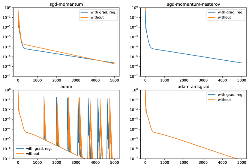
Figure 2: Overview of optimizer loss curves for one polynomial with $\lambda=1$.

With our degree-based regularization approach introduced in section 3.1, SGD with momentum is able to converge quicker and we are able to use Nesterov momentum, which was not possible otherwise. We achieved best results with an SGD momentum setting of $0.95$ and AMSGrad $\beta_{1}$ = 0.9, $\beta_{2}$=0.999 and $\epsilon=10^{-7}$. On that basis, we investigated our general spline model, by we sweeping $\lambda$ from $1$ to $0$. Experiments show that both optimizers are able to generate near $\mathcal{C}^{2}$-continuos results across the observed $\lambda$-range while at the same time delivering favorable approximation results. The remaining continuity correction errors for the algorithm introduced in section 3.3 to process are small.

Using $\mathcal{C}^{2}$-splines of degree $5$, again, AMSGrad has a better performance compared to SGD. For all tested $0<\lambda<1$, SGD and AMSGrad manage to produce splines of low loss within 10 000 epochs: SGD reaches $\ell\approx 10^{-4}$ and AMSGrad reaches $\ell\approx 10^{-6}$. Given an application-specific tolerance, we may already stop after a few hundred epochs.

5 Conclusion and Outlook

We have presented an “out-of-the-box” application of ML optimizers for the industrial optimization problem of cam approximation. The model introduced in section 2.1 and extended by practical considerations in section 3.2 allows for fitting of $\mathcal{C}^{k}$-continuos splines, which can be deployed in a cam approximation setting. Our experiments documented in section 4 show that the problem solution is feasible using TensorFlow gradient tapes and that AMSGrad and SGD show the best results among available TensorFlow optimizers. Our gradient regularization approach introduced in section 3.1 improves SGD convergence and allows usage of SGD with Nesterov momentum. Although experiments show that remaining discontinuities after optimization are small, we can eliminate these errors using the algorithm introduced in section 3.3, which has impact only on affected derivatives in the local spline segment.

Additional terms in $\ell$ can accommodate for further domain-specific goals. For instance, we can reduce oscillations in $f$ by penalizing the strain energy

$$\ell_{\text{strain}}=\int_{I}f^{\prime\prime}(x)^{2}\;\mathrm{d}{x}\,.$$

In our experiments outlined in the previous section, we started with all polynomial coefficients initialized to zero to investigate convergence. To improve convergence speed in future experiments, we can start with the $\ell_{2}$-optimal spline and let our method minimize the overall goal $\ell$.

Flexibility of our method with regards to the underlying polynomial model allows for usage of different function types. In this way, as an example, an orthogonal basis using Chebyshev polynomials could improve convergence behavior compared to classical monomials.

References

- [1] Adcock, B., Dexter, N.: The gap between theory and practice in function approximation with deep neural networks. SIAM Journal on Mathematics of Data Science 3(2), 624–655 (2021). https://doi.org/10.1137/20M131309X
- [2] Reddi, S.J., Kale, S., Kumar, S.: On the convergence of adam and beyond. CoRR abs/1904.09237 (2019). https://doi.org/10.48550/arXiv.1904.09237
- [3] Sandgren, E., West, R.L.: Shape optimization of cam profiles using a b-spline representation. Journal of Mechanisms, Transmissions, and Automation in Design 111(2), 195–201 (06 1989). https://doi.org/10.1115/1.3258983
- [4] TensorFlow: Built-in optimizer classes. https://www.tensorflow.org/api_docs/python/tf/keras/optimizers (2022), accessed: 2022-02-28
- [5] Waclawek, H., Huber, S.: Spline approximation with tensorflow gradient descent optimizers for use in cam approximation. https://github.com/hawaclawek/tf-for-splineapprox (2022), accessed: 2022-05-31